A Stable Mixed FE Method for Nearly Incompressible Linear Elastostatics

Abstract

[Summary] We present a new, stable, mixed finite element (FE) method for linear elastostatics of nearly incompressible solids. The method is the automatic variationally stable FE (AVS-FE) method of Calo, Romkes and Valseth, in which we consider a Petrov-Galerkin weak formulation where the stress and displacement variables are in the space $H(\bf{div})$ and $H^{1}$, respectively. This allows us to employ a fully conforming FE discretization for any elastic solid using classical FE subspaces of $H(\bf{div})$ and $H^{1}$. Hence, the resulting FE approximation yields both continuous stresses and displacements.

To ensure stability of the method, we employ the philosophy of the discontinuous Petrov-Galerkin (DPG) method of Demkowicz and Gopalakrishnan and use optimal test spaces. Thus, the resulting FE discretization is stable even as the Poisson’s ratio $\nu\rightarrow 0.5$, and the system of linear algebraic equations is symmetric and positive definite. Our method also comes with a built-in a posteriori error estimator as well as indicators which are used to drive mesh adaptive refinements. We present several numerical verifications of our method including comparisons to existing FE technologies.

1 Introduction

Linear elastostatics is arguably the most successful area of application of the classical (Bubnov-Galerkin) FE method. For homogeneous isotropic engineering materials, such as steel and aluminum, the Bubnov-Galerkin method is stable, satisfies a best approximation property in terms of elastic strain energy and is computationally efficient. However, for commonly employed modern engineering materials such as rubbers and soft plastics, i.e., nearly incompressible materials, the Bubnov-Galerkin method suffers from locking and loss of discrete stability (see, e.g., ^{1, 2, 3}). In ⁴, Phillips and Wheeler investigate this phenomenon in great detail and highlight that error estimates for the classical FE method depend on the factor $1/(1-2\nu)$, which clearly tends to infinity as $\nu\rightarrow 0.5$.

Mixed FE methods ⁵ provide functional settings in which certain FE discretizations are stable for mixed forms of the elastostatics problem as well as for the Stokes equations which and can be shown to be equivalent to the equations of linear elastostatics when $\nu=0.5$. Other mixed FE methods based on the consideration of the underlying equations of elastostatics using the compliance tensor do not suffer from this loss of stability, but often require additional constraints to ensure symmetric stresses ⁶, called Hellinger-Reissner formulations, and are typically more computationally costly than the primal Bubnov-Galerkin formulation. In ⁷, Arnold and Winther present an element for the Hellinger-Reissner formulation which was one of the first stable elements utilizing polynomial bases for both stress and displacement. The difficulty in building conforming approximation spaces for the stress has also resulted in several nonconforming mixed methods, see e.g., ^{8, 9} where the FE approximation of the stress does not reside in the space dictated by the weak formulation. The task of establishing approximation spaces for these mixed FE methods is certainly not trivial and is an active area of investigation and recent publications include ^{10, 11}.

Stabilized FE methods that adjust the functionals of the weak formulation can be used to ensure discrete stability ¹². This type of stabilization is performed for both the mixed and classical FE methods, see the work of Nakshatrala et al. ¹³ as well as Masud et al. ¹⁴. However, stabilized methods generally require arduous analyses to establish a proper choice of penalization/stabilization parameters. Reduced integration methods are also commonly used when approaching the incompressible limit ¹⁵. The discontinuous Galerkin (DG) method also remains a popular choice for nearly incompressible elastostatics ^{16, 4, 17}. In general, these achieve stability by adjusting the inter-element jump or average terms by weights in a manner similar to the stabilized FE methods.

Stable FE methods such as the least squares FE methods (LSFEMs) (see, e.g., text by Bochev and Gunzberger ¹⁸) or the discontinuous Petrov-Galerkin (DPG) Method of Demkowicz and Gopalakrishnan ¹⁹ can be employed to resolve the stability issue. The LSFEM has been applied to linear elastostatics in ²⁰ and in ²¹, a weighted first-order system least squares is applied successfully to nearly incompressible materials. Gopalakrishnan and Qiu provide an analysis of the well-posedness of the DPG method applied to linear elastostatics in ²². In ²³, Bramwell et al. consider two distinct DPG methods for the nearly incompressible elastostatics problem that are locking free and present numerical verifications highlighting capabilities as $\nu\rightarrow 0.5$. The DPG has also been successfully applied to this problem in several works, including the fully incompressible case in ²⁴ employing the compliance tensor to avoid locking in that case. In ^{24, 25}, the DPG method is applied to the problem of linear elastostatics and several variational formulations are considered including for the case of nearly incompressible materials. In particular, in ²⁴, the idea of coupling multiple weak formulations throughout the computational domain is explored in great detail.

In the classical FE method, the approximations of displacements of the equivalent weak form of the underlying partial differential equation (PDE) of static equilibrium are sought in $C^{0}$ continuous polynomial spaces and stress approximations are established by computing gradients of the displacements, i.e., the stresses are piecewise discontinuous. On the other hand, mixed FE methods for the linear elastostatics problem consider an equivalent first-order system of the underlying PDE. This first-order system description can lead to weak forms which allow stresses to be in $H(\text{\bf{div}},\Omega)$ and displacements that are in $L^{2}(\Omega)$ (see Section 2.4 of ²⁵ for a thorough discussion on other options). Hence, in the FE approximations the displacements must be sought in piecewise discontinuous polynomial function spaces. The theory of distributions ensures that optimally convergent FE solutions can be established for both classical and mixed FE methods, as well as for their properly stabilized counterparts if $\nu$ is close to $0.5$. However, the resulting numerical approximations are not physical, as we know that both the displacement and certain components of the stress fields are continuous. We know of three options to establish both continuous displacements and stresses. Firstly, the isogeometric FE methods of Hughes et al. ²⁶ which uses higher order bases for the discrete FE approximation, i.e., $C^{k}$ continuity. Secondly, the $k-$version FE method of Surana et al. ²⁷ which employs higher order bases as well as a least squares approach. The popularity of the isogeometric FE method has grown significantly over the last decade, but the stability issue of nearly incompressible materials still persist. In ²⁸, Taylor introduces a mixed version of the isogeometric FE methods for incompressible solids where discontinuous stress approximations are sought. Lastly, the use of post processing techniques where a discontinuous solution component is projected into a continuous discrete space, e.g., by using Oswald operators, see ^{29, 30} for details and further references.

The automatic variationally stable finite element (AVS-FE) method introduced by Calo, Romkes and Valseth in ³¹ provides a framework, much like the DPG of Demkowicz and Gopalakrishnan ¹⁹, to establish stable FE approximations for any PDE. However, the AVS-FE differs in its choice of trial spaces while employing the DPG concept of optimal discontinuous test functions. In addition to the approximation of the trial variables, the AVS-FE also comes with a "built-in" error estimator and error indicators that can be employed to drive mesh adaptive strategies. The stability property of the AVS-FE allows us to derive Petrov-Galerkin weak formulations that are posed with trial functions that are in classical Hilbert spaces, e.g., $H(\bf{div})$ and $H^{1}$. Hence, the corresponding FE approximations are to be sought in classical continuous FE approximation spaces yielding continuous FE approximations for all trial variables. The LSFEMs presented in ^{20, 21} also pose weak formulations in Hilbert spaces as the AVS-FE but considers alternative formulations for the elasticity problem and considers nonconforming approximations for the displacement.

In this paper, we build upon the preliminary investigation of Valseth in ³² for the AVS-FE method applied to linear elastostatics of nearly incompressible media. We introduce our model problem and notations in Section 2.1, The weak formulation and its corresponding FE discretzation are presented in Section 2 in conjunction with a brief review of the AVS-FE methodology. In Section 2.4, we present optimal a priori error estimates. Several numerical verifications are presented in Section 3 highlighting the stability of our method as $\nu\rightarrow 0.5$, including an asymptotic convergence study with comparisons to existing FE methods. We draw conclusions and discuss future works in Section 4.

2 The AVS-FE Method

The AVS-FE method ³¹ provides a functional setting to analyze linear boundary value problems (BVPs) in which the underlying differential operator is non self-adjoint or leads to unstable FE discretizations. In this section we introduce our model problem, and briefly review the AVS-FE method. A thorough introduction can be found in  ³¹.

2.1 Model Problem: Linear Elastostatics of Nearly Incompressible Solids

Let $\Omega\subset\mathbb{R}^{{\color[rgb]{0,0,0}n}}$, $n=1,2,3$ (we consider the two dimensional case here for simplicity) be a bounded open domain, containing a linearly elastic, nearly incompressible, and possible heterogeneous solid. The boundary $\partial\Omega$ is partitioned into two open and disjoint segments ${\Gamma_{t}}$ and ${\Gamma_{\mathbf{u}}}$, such that $\partial\Omega=\overline{{\Gamma_{t}}\cup{\Gamma_{\mathbf{u}}}}$. As depicted in Figure 1, the body is in static equilibrium under the action of external body loads $\mathbf{f}\in[L^{2}(\Omega)]^{2}$ in $\Omega$, surface tractions $\mathbf{t}\in{H^{-1/2}({\Gamma_{t}})}$ on ${\Gamma_{t}}$, as well as fixed zero displacements on ${\Gamma_{\mathbf{u}}}$. Since the solid is assumed to be linearly elastic, its constitutive behavior is governed by Generalized Hooke’s Law, i.e.:

$$\boldsymbol{\sigma}=\mathbf{E}\,\boldsymbol{\varepsilon},$$ (1)

where $\boldsymbol{\sigma}$ denotes the (2D) Cauchy stress tensor, $\boldsymbol{\varepsilon}$ the (2D) Green strain tensor, and $\mathbf{E}$ the fourth order (Riemann) elasticity tensor, with elliptic and symmetric Riemann coefficients $E_{ijkl}\in{L^{\infty}(\Omega)}$. In this work, we limit our focus to problems in which the deformations in the material remain small and therefore the kinematic relation between the strain tensor $\boldsymbol{\varepsilon}$ and displacement field $\mathbf{u}$ is linear and governed by:

$$\boldsymbol{\varepsilon}=\frac{1}{2}\left[\boldsymbol{\nabla}\mathbf{u}+(\boldsymbol{\nabla}\mathbf{u})^{T}\right].$$ (2)

With these notations and relations in force, the equilibrium state of the solid is represented by the following BVP, governing the displacement field $\mathbf{u}$:

$$\boxed{\begin{array}[]{l}\text{Find}\;\mathbf{u}\in{\color[rgb]{0,0,0}[H^{1}(\Omega)]^{2}}\;\text{such that:}\\ \\[-7.22743pt] \hskip 36.135pt\begin{array}[]{rcll}-\boldsymbol{\nabla}\cdot{\color[rgb]{0,0,0}\boldsymbol{\sigma}}&=&\mathbf{f},&\text{in}\;\Omega,\\[7.22743pt] {\color[rgb]{0,0,0}\boldsymbol{\sigma}}\mathbf{n}&=&\mathbf{t},&\text{on}\;{\Gamma_{t}},\\ \mathbf{u}&=&\mathbf{0},&\text{on}\;{\Gamma_{\mathbf{u}}},\end{array}\end{array}}$$ (3)

where $\mathbf{n}$ denotes the outward unit normal vector to $\partial\Omega$. In this paper, we consider the specific scenario in which the solid is comprised of one or more constituents with nearly incompressible material properties. Hence, the Riemann coefficients $E_{ijkl}$ can involve values of the Poisson Ratio $\nu$ that are very close to, but still less than, $0.5$.

Figure 1: The model problem.

In the following, we shall use the following notations:

• inner products between vector valued functions are denoted with the single dot symbol $\cdot$, and inner products between tensor valued functions are denoted by the colon or double dot symbol $\colon$.

• $h_{m}$ is the diameter of element $K_{m}$.

• in weak formulations, we present edge integrals using trace the operators: $i)$ $\gamma^{m}_{0}:H^{1}(K_{m}):\longrightarrow H^{1/2}(\partial K_{m})$ as the local zeroth order trace operator and $ii)$ $\gamma^{m}_{\mathbf{n}_{m}}:H(\text{\bf{div}},K_{m})\longrightarrow H^{-1/2}(\partial K_{m})$ denote the local normal trace operators where $\mathbf{n}_{m}$ is the outward unit normal vector to the element boundary $\partial K_{m}$ (e.g., see ³³).

• vector and tensor valued test functions are denoted using $\mathbf{v}$ and $\mathbf{w}$, respectively. Restrictions of these to an element $K_{m}$ are denoted by employing the subscript $m$.

2.2 Weak Formulation

AVS-FE weak formulations are established using techniques that are similar to DG and DPG methods by considering element-wise weak formulations that are subsequently summed throughout the FE mesh partition to yield global weak formulations. We mention only key points here and omit the full derivation here for brevity but refer to ³¹ for detailed derivations.

To establish AVS-FE weak formulations, we first require a partition $\mathcal{P}_{h}$ of $\Omega$ into convex elements $K_{m}$, such that:

$$\Omega=\text{int}(\bigcup_{K_{m}\in\mathcal{P}_{h}}\overline{K_{m}}),\quad K_{m}\cap K_{n}{\color[rgb]{0,0,0}=0},\quad m\neq n.$$

The partition $\mathcal{P}_{h}$ is such that any discontinuities in $E_{ijkl}$ are restricted to the boundaries of each element $\partial K_{m}$. The BVP (3) is recast as a first-order system by using the stress tensor from the constitutive law (1), i.e.,

$$\boxed{\begin{array}[]{l}\text{Find}\;(\mathbf{u},\boldsymbol{\sigma})\in{\color[rgb]{0,0,0}[H^{1}(\Omega)]^{2}}\times H(\text{\bf{div}},\Omega)\;\text{such that:}\\ \\[-7.22743pt] \hskip 36.135pt\begin{array}[]{rcll}\boldsymbol{\sigma}-\mathbf{E}\,\boldsymbol{\varepsilon}&=&\mathbf{0}&\text{in}\;\Omega,\\ -\boldsymbol{\nabla}\cdot\boldsymbol{\sigma}&=&\mathbf{f},&\text{in}\;\Omega,\\[7.22743pt] \boldsymbol{\sigma}\,\mathbf{n}&=&\mathbf{t},&\text{on}\;{\Gamma_{t}},\\ \mathbf{u}&=&\mathbf{0},&\text{on}\;{\Gamma_{\mathbf{u}}},\end{array}\end{array}}$$ (4)

where $H(\text{\bf{div}},\Omega)$ is the Hilbert space of tensor-valued functions which divergence is weakly continuous and $\boldsymbol{\varepsilon}=\boldsymbol{\varepsilon}(\mathbf{u})$ denotes the gradient operator in (2). Note that this first-order system, or mixed form, BVP is standard for mixed FE methods for linear eleastostatics.

Next, the first-order system is multiplied by test functions $(\mathbf{v},\mathbf{w})\in L^{2}(K_{m})^{6}$ and enforced weakly on each individual element $K_{m}\in\mathcal{P}_{h}$. We then apply integration by parts locally on each element $K_{m}$ to the term involving the divergence of the stress field $\boldsymbol{\nabla}\cdot\boldsymbol{\sigma}$ to enable weak applications of the Neumann boundary condition (BC). A subsequent summation of all elements in $\mathcal{P}_{h}$ and strong enforcement of all BCs leads us to the AVS-FE weak formulation:

$$\boxed{\begin{array}[]{ll}\text{Find }(\mathbf{u},\boldsymbol{\sigma})\in U(\Omega)\text{ such that:}\\[3.61371pt] \qquad B((\mathbf{u},\boldsymbol{\sigma}),(\mathbf{v},\mathbf{w}))=F(\mathbf{v}),\quad\forall(\mathbf{v},\mathbf{w})\in{V(\mathcal{P}_{h})},\end{array}}$$ (5)

where the test space ${V(\mathcal{P}_{h})}$ is broken, the bilinear form, $B:U(\Omega)\times{V(\mathcal{P}_{h})}\longrightarrow\mathbb{R}$, and linear functional, $F:{V(\mathcal{P}_{h})}\longrightarrow\mathbb{R}$ are defined:

$$\begin{array}[]{c}B((\mathbf{u},\boldsymbol{\sigma}),(\mathbf{v},\mathbf{w}))\overset{\text{def}}{=}\displaystyle\overset{}{\underset{K_{m}\in\mathcal{P}_{h}}{\sum}}\biggl{\{}\int_{K_{m}}\biggl{[}\,\left(\boldsymbol{\sigma}-\mathbf{E}\boldsymbol{\varepsilon}(\mathbf{u})\right){\color[rgb]{0,0,0}:}\mathbf{w}_{m}\,+\,\boldsymbol{\sigma}:\boldsymbol{\nabla}\mathbf{v}_{m}\biggr{]}\;{\rm d}\mathbf{x}\biggr{.}\oint_{\partial K_{m}}\gamma^{m}_{\mathbf{n}}(\boldsymbol{\sigma})\,\gamma^{m}_{0}(\mathbf{v}_{m})\,\,{\rm d}s\biggr{\}},\\[10.84006pt] F(\mathbf{v})\overset{\text{def}}{=}\displaystyle\overset{}{\underset{K_{m}\in\mathcal{P}_{h}}{\sum}}\int_{K_{m}}\mathbf{f}\cdot\mathbf{v}_{m}\;{\rm d}\mathbf{x},\end{array}$$ (6)

and the function spaces are defined:

$$\begin{array}[]{c}U(\Omega)\overset{\text{def}}{=}\biggl{\{}(\mathbf{u},\boldsymbol{\sigma})\in{\color[rgb]{0,0,0}[H^{1}(\Omega)]^{2}}\times H(\text{\bf{div}},\Omega):\;\gamma_{0}^{m}(\mathbf{u})_{|\partial K_{m}\cap{\Gamma_{\mathbf{u}}}}=\mathbf{0},{\color[rgb]{0,0,0}\gamma_{0}^{m}(\boldsymbol{\sigma})_{|\partial K_{m}\cap{\Gamma_{t}}}=\mathbf{t}}\;\forall K_{m}\in\mathcal{P}_{h}\biggr{\}},\\[10.84006pt] {V(\mathcal{P}_{h})}\overset{\text{def}}{=}\biggl{\{}(\mathbf{v},\mathbf{w})\in[H^{1}(\mathcal{P}_{h})]^{2}\times[L^{2}(\Omega)]^{4}:\,\gamma_{0}^{m}(\mathbf{v}_{m})_{|\partial K_{m}\cap{\Gamma_{\mathbf{u}}}}=\mathbf{0},\;\forall K_{m}\in\mathcal{P}_{h}\biggr{\}},\end{array}$$ (7)

with norms $\|{\cdot}\|_{U(\Omega)}:U(\Omega)\!\!\longrightarrow\!\![0,\infty)$ and $\|{\cdot}\|_{{V(\mathcal{P}_{h})}}:{V(\mathcal{P}_{h})}\!\!\longrightarrow\!\![0,\infty)$ defined as:

$$\begin{array}[]{l}\displaystyle\|{(\mathbf{u},\boldsymbol{\sigma})}\|_{U(\Omega)}\overset{\text{def}}{=}\sqrt{\int_{\Omega}\biggl{[}\boldsymbol{\nabla}\mathbf{u}:\boldsymbol{\nabla}\mathbf{u}+\mathbf{u}\cdot\mathbf{u}+(\boldsymbol{\nabla}\cdot\boldsymbol{\sigma})^{2}+\boldsymbol{\sigma}\cdot\boldsymbol{\sigma}\biggr{]}\;{\rm d}\mathbf{x}},\\[14.45377pt] \displaystyle\|{(\mathbf{v},\mathbf{w})}\|_{{V(\mathcal{P}_{h})}}\overset{\text{def}}{=}\sqrt{\overset{}{\underset{K_{m}\in\mathcal{P}_{h}}{\sum}}\int_{K_{m}}\biggl{[}h_{m}^{2}\boldsymbol{\nabla}\mathbf{v}_{m}:\boldsymbol{\nabla}\mathbf{v}_{m}+\mathbf{v}_{m}\cdot\mathbf{v}_{m}+\mathbf{w}_{m}:\mathbf{w}_{m}\biggr{]}\;{\rm d}\mathbf{x}}.\end{array}$$ (8)

The norm $\|{\cdot}\|_{{V(\mathcal{P}_{h})}}$ is equivalent to the $L^{2}$ norm:

$$\begin{array}[]{l}\displaystyle\|{(\mathbf{v},\mathbf{w})}\|_{L^{2}(\Omega)}{\color[rgb]{0,0,0}=}\sqrt{\int_{{\color[rgb]{0,0,0}\Omega}}\biggl{[}{\color[rgb]{0,0,0}\mathbf{v}}\cdot{\color[rgb]{0,0,0}\mathbf{v}}+\mathbf{w}:\mathbf{w}\biggr{]}\;{\rm d}\mathbf{x}}.\end{array}$$ (9)

Note that the edge integrals in (6) are to be interpreted as duality pairings in $H^{1/2}(\partial K_{m})\times H^{-1/2}(\partial K_{m})$, but we employ notation that is engineering convention here using the integral representation. Most importantly, since $(\mathbf{u},\boldsymbol{\sigma})\in{\color[rgb]{0,0,0}[H^{1}(\Omega)]^{2}}\times H(\text{\bf{div}},\Omega)$, these integrals are well defined and our trial space is continuous. As the trial and test spaces are of different regularity we are in a Petrov-Galerkin setting, particularly a DPG setting, since the test space is broken. However, since the trial space is ${\color[rgb]{0,0,0}[H^{1}(\Omega)]^{2}}\times H(\text{\bf{div}},\Omega)$ our functional setting differs from that of DPG methods in which the regularity of the trial space is reduced by introducing variables on the edge of each element.

Remark 2.1.

The norm $\|{\cdot}\|_{{V(\mathcal{P}_{h})}}$ is used in the discrete computational setting due to exhaustive numerical experimentation. In particular, its use is justified based on $i)$ engineering and $ii)$ computational intuition. $i)$ The scaling ensures consistency of units, e.g., if $\mathbf{v}$ is of unit length then $\boldsymbol{\nabla}\mathbf{v}$ is of unit $\frac{1}{\text{length}}$. Thus, all entries are of the same unit. $ii)$ The scaling also ensures that all terms in the norm are of the same magnitude in the discrete setting due to the exact same reasoning since gradient terms scale as $h^{-1}$. Finally we note that the equivalence between $\|{\cdot}\|_{{V(\mathcal{P}_{h})}}$ and $\|{\cdot}\|_{L^{2}(\Omega)}$ is based on mesh dependent constants.

In the spirit of the DPG method, we now introduce an equivalent norm on the trial space, the energy norm $\|{\cdot}\|_{\text{B}}:U(\Omega)\longrightarrow[0,\infty)$:

$$\|{(\mathbf{u},\boldsymbol{\sigma})}\|_{\text{B}}\overset{\text{def}}{=}\underset{(\mathbf{v},\mathbf{w})\in{V(\mathcal{P}_{h})}\setminus\{(\mathbf{0},\mathbf{0})\}}{\sup}\,\frac{|B(\mathbf{u},\boldsymbol{\sigma}),(\mathbf{v},\mathbf{w}))|}{\quad\|{(\mathbf{v},\mathbf{w})}\|_{{V(\mathcal{P}_{h})}}},$$ (10)

and a Riesz representation problem for $(\mathbf{p},\mathbf{r})$, the optimal test functions:

$$\begin{array}[]{rcll}\displaystyle\left(\,(\mathbf{p},\mathbf{r}),(\mathbf{v},\mathbf{w})\,\right)_{V(\mathcal{P}_{h})}&\!\!=\!&B(\,(\mathbf{u},\boldsymbol{\sigma}),(\mathbf{v},\mathbf{w})\,),&\,\forall({\color[rgb]{0,0,0}\mathbf{v}},\mathbf{w})\in{V(\mathcal{P}_{h})}.\end{array}$$ (11)

The Riesz representation problem is well posed with unique solutions due to the inner product in the left hand side (LHS) and guarantees the stability of DPG methods. The Riesz representation problem also leads to the following norm equivalence:

$$\|{(\mathbf{u},\boldsymbol{\sigma})}\|_{\text{B}}=\|{(\mathbf{p},\mathbf{r})}\|_{{V(\mathcal{P}_{h})}},$$ (12)

which will be employed extensively in the following. For details on optimal test functions and proof of the norm equivalence, we refer to ^{34, 19}. Due to the energy norm, the bilinear form (6) has continuity and inf-sup constants equal to one and the load functional is also continuous which can be shown using classical techniques. Hence, we have established a well posed weak formulation of the linear elastostatics BVP using continuous trial spaces for both displacement and stress fields, i.e., ${\color[rgb]{0,0,0}[H^{1}(\Omega)]^{2}}\times H(\text{\bf{div}},\Omega)$, in terms of the energy norm (10).

Well-posedness in terms of the energy norm is essentially an assumption of DPG methods as we define a norm that ensure inf-sup and continuity conditions of the bilinear form. For completeness, we also provide the following lemma of well-posedness in standard Sobolev norms by first stating two important results. For the sake of simplicity, we consider the case in which homogeneous Dirichlet BCs are applied on the full boundary $\partial\Omega={\Gamma_{\mathbf{u}}}$:

Proposition 2.1.

Let $(\mathbf{u}^{\rm{D}},\boldsymbol{\sigma}^{\rm{D}})\in[H^{1}_{{\Gamma_{\mathbf{u}}}}(\Omega)]^{2}\times[L^{2}(\Omega)]^{4}$ be the solution of the dual mixed formulation:

$$\begin{array}[]{ll}\text{Find }(\mathbf{u}^{\text{D}},\boldsymbol{\sigma}^{\text{D}})\in[H^{1}_{{\Gamma_{\mathbf{u}}}}(\Omega)]^{2}\times[L^{2}(\Omega)]^{4}\text{ such that:}\\[3.61371pt] \displaystyle\quad\underbrace{\int_{\Omega}\biggl{[}\left(\boldsymbol{\sigma}^{\text{D}}-\mathbf{E}\boldsymbol{\varepsilon}(\mathbf{u}^{\text{D}})\right){\color[rgb]{0,0,0}:}\mathbf{w}+\boldsymbol{\sigma}^{\text{D}}:\boldsymbol{\nabla}\mathbf{v}\biggr{]}\;{\rm d}\mathbf{x}}_{b^{\text{D}}(\mathbf{u}^{\text{D}},\boldsymbol{\sigma}^{\text{D}}),(\mathbf{v},\mathbf{w}))}=\int_{\Omega}\mathbf{f}\cdot\mathbf{v}\;{\rm d}\mathbf{x},\quad\forall(\mathbf{v},\mathbf{w})\in[H^{1}_{{\Gamma_{\mathbf{u}}}}(\Omega)]^{2}\times[L^{2}(\Omega)]^{4},\end{array}$$ (13)

which is well posed. Hence, the bilinear form satisfies the inf-sup condition:

$$\begin{array}[]{l}\exists\gamma>0:\underset{(\mathbf{v},\mathbf{w})\in{V(\Omega)}}{\sup}\,\displaystyle\frac{|b^{\text{D}}(\mathbf{u}^{\text{D}},\boldsymbol{\sigma}^{\text{D}}),(\mathbf{v},\mathbf{w}))|}{\|{(\mathbf{v},\mathbf{w})}\|_{{V(\Omega)}}}\geq\gamma\,\|{(\mathbf{u}^{\text{D}},\boldsymbol{\sigma}^{\text{D}})}\|_{U^{D}(\Omega)},\end{array}$$ (14)

where $U^{D}(\Omega)={V(\Omega)}=[H^{1}_{{\Gamma_{\mathbf{u}}}}(\Omega)]^{2}\times[L^{2}(\Omega)]^{4}$ and $H^{1}_{{\Gamma_{\mathbf{u}}}}(\Omega)$ is the space of $H^{1}$ functions that satisfy homogeneous Dirichlet conditions on ${\Gamma_{\mathbf{u}}}=\partial\Omega$.

Proof: see Theorem 2.1 in ²⁵.
 ∎

We write the bilinear form (6) as:

$$\begin{array}[]{l}B((\mathbf{u},\boldsymbol{\sigma}),(\mathbf{v},\mathbf{w}))=b^{\text{D}}((\mathbf{u},\boldsymbol{\sigma}),(\mathbf{v},\mathbf{w}))+\big{\langle}{\gamma^{m}_{\mathbf{n}}(\boldsymbol{\sigma})},{\gamma^{m}_{0}(\mathbf{v})}\big{\rangle}_{\Gamma_{h}},\end{array}$$ (15)

where $\big{\langle}{\gamma^{m}_{\mathbf{n}}(\boldsymbol{\sigma})},{\gamma^{m}_{0}(\mathbf{v})}\big{\rangle}_{\Gamma_{h}}\overset{\text{def}}{=}\overset{}{\underset{K_{m}\in\mathcal{P}_{h}}{\sum}}\oint_{\partial K_{m}}\{\gamma^{m}_{\mathbf{n}}(\boldsymbol{\sigma})\,,\gamma^{m}_{0}(\mathbf{v}_{m})\,\}\,{\rm d}s$.

Proposition 2.2.

Let $\boldsymbol{\sigma}\in H({\color[rgb]{0,0,0}\text{\bf{div}}},\mathcal{P}_{h})$ and ${\color[rgb]{0,0,0}\mathbf{v}}\in{\color[rgb]{0,0,0}[H^{1}(\mathcal{P}_{h})]^{2}}$. Then:

$$\begin{array}[]{l}\exists\gamma^{S}>0:\underset{{\color[rgb]{0,0,0}\mathbf{v}_{m}}\in{\color[rgb]{0,0,0}[H^{1}(\mathcal{P}_{h})]^{2}}}{\sup}\,\displaystyle\frac{|\big{\langle}{\gamma^{m}_{\mathbf{n}}(\boldsymbol{\sigma})},{\gamma^{m}_{0}(\mathbf{v}_{m})}\big{\rangle}_{\Gamma_{h}}|}{\|{{\color[rgb]{0,0,0}\mathbf{v}}}\|_{H^{1}(\mathcal{P}_{h})}}\geq\gamma^{S}\,\|{\boldsymbol{\sigma}}\|_{\hat{U}(\Gamma_{h})},\end{array}$$ (16)

where $H({\color[rgb]{0,0,0}\text{\bf{div}}},\mathcal{P}_{h})$ denotes the broken $H(\bf{div})$ space and $\|{\boldsymbol{\sigma}}\|_{\hat{U}(\Gamma_{h})}$ is the minimum energy extension norm:

$$\begin{array}[]{l}\|{\boldsymbol{\sigma}}\|_{\hat{U}(\Gamma_{h})}\overset{\text{def}}{=}\displaystyle\underset{{\color[rgb]{0,0,0}\mathbf{v}}\in{\color[rgb]{0,0,0}[H^{1}(\mathcal{P}_{h})]^{2}}}{\sup}\,\displaystyle\frac{|\big{\langle}{\gamma^{m}_{\mathbf{n}}(\boldsymbol{\sigma})},{\gamma^{m}_{0}(\mathbf{v}_{m})}\big{\rangle}_{\Gamma_{h}}|}{\|{{\color[rgb]{0,0,0}\mathbf{v}}}\|_{H^{1}(\mathcal{P}_{h})}}=\,\rm{inf}\,\|{\boldsymbol{\sigma}}\|_{H(\text{\bf{div}},\Omega)}.\end{array}$$ (17)

Additionally, if $\boldsymbol{\sigma}\in H(\text{\bf{div}},\Omega)$:

$$\begin{array}[]{l}\big{\langle}{\gamma^{m}_{\mathbf{n}}(\boldsymbol{\sigma})},{\gamma^{m}_{0}(\mathbf{v})}\big{\rangle}_{\Gamma_{h}}=0,\quad{\color[rgb]{0,0,0}\forall\mathbf{v}\in H^{1}(\Omega)}.\end{array}$$ (18)

Proof: see Theorem 2.3 in ³⁵.
 ∎

Lemma 2.1.

Let $(\mathbf{u},\boldsymbol{\sigma})\in U(\Omega)$ and $(\mathbf{v},\mathbf{w})\in{V(\mathcal{P}_{h})}$. Then, the AVS-FE weak formulation (5) satisfies all conditions of the Babuška Lax-Milgram Theorem ³⁶ and is well posed.

Proof: The load functional and bilinear form (6) are continuous due to the Cauchy-Schwarz inequality. The following inf-sup condition:

$$\begin{array}[]{l}\exists C>0:\underset{(\mathbf{v},\mathbf{w})\in{V(\mathcal{P}_{h})}}{\sup}\,\displaystyle\frac{|B(\mathbf{u},\boldsymbol{\sigma}),(\mathbf{v},\mathbf{w}))|}{\|{(\mathbf{v},\mathbf{w})}\|_{{\color[rgb]{0,0,0}W(\mathcal{P}_{h})}}}\geq\gamma\,\|{(\mathbf{u},\boldsymbol{\sigma})}\|_{U(\Omega)},\end{array}$$ (19)

is satisfied due to Theorem 3.3 in ³⁵. This theorem holds if the following conditions hold (see Assumptions 3.1 and 3.2 in ³⁵): $i)$ the bilinear form $b^{\text{D}}(\cdot,\cdot)$ satisfies the inf-sup condition and has a trivial kernel, the form $\big{\langle}{\gamma^{m}_{\mathbf{n}}(\boldsymbol{\sigma})},{\gamma^{m}_{0}(\mathbf{v})}\big{\rangle}_{\Gamma_{h}}$ satisfies $ii)$ an inf-sup condition and $iii)$ a kernel preserving property. Due to Proposition 2.1, we can conclude that the bilinear form $b^{\text{D}}(\cdot,\cdot)$ satisfies $i)$. Second, $\big{\langle}{\gamma^{m}_{\mathbf{n}}(\boldsymbol{\sigma})},{\gamma^{m}_{0}(\mathbf{v})}\big{\rangle}_{\Gamma_{h}}$ satisfies the inf-sup condition in (16), and the kernel preserving property is satisfied by noting that $\big{\langle}{\gamma^{m}_{\mathbf{n}}(\boldsymbol{\sigma})},{\gamma^{m}_{0}(\mathbf{v})}\big{\rangle}_{\Gamma_{h}}$ vanishes if evaluated using test functions from the test space of $b^{\text{D}}(\cdot,\cdot)$. The norm in the denominator is defined: $\|{(\mathbf{v},\mathbf{w})}\|_{{\color[rgb]{0,0,0}W(\mathcal{P}_{h})}}^{2}=\|{\mathbf{v}}\|_{H^{1}(\mathcal{P}_{h})}^{2}+\|{\mathbf{w}}\|_{L^{2}(\Omega)}^{2}$.
 ∎

Remark 2.2.

The bilinear and linear forms in (6) are not unique choices for the AVS-FE method. We have chosen these particular forms as they allow us to keep the weak formulation close to classical mixed FE methods for linear elastostatics and enforce Dirichlet BCs strongly and Neumann BCs weakly. Other forms can be derived in which the trial space is continuous, and the test space is discontinuous, due to the flexibility of the Petrov-Galerkin method. In ²⁵ Keith et al. consider several possible weak formulations for the elastostatics problem and the DPG method and perform a rigorous analysis showing their well posedness.

2.3 AVS-FE Discretization

To establish FE discretizations of the weak formulation (5), the AVS-FE takes the approach of classical FE methods and seeks continuous polynomial approximations that are in conforming subspaces of the ${\color[rgb]{0,0,0}[H^{1}(\Omega)]^{2}}\times H(\text{\bf{div}},\Omega)$ trial spaces. Hence, for the displacement field we use classical $C^{0}(\Omega)$ continuous Lagrange polynomials. Generally, in mixed FE methods this choice leads to unstable and inconsistent FE discretizations and is avoided and the stress field is sought in a Raviart-Thomas (RT) or Brezzi-Douglas-Marini (BDM) space ⁵. Due to the stability properties of the AVS-FE method, it is often convenient to employ the same $C^{0}(\Omega)$ polynomials for the stress variable. As reported in ³⁷, for convex domains and smooth solutions, the $C^{0}(\Omega)$ are superior. In Section 3 we present numerical verifications comparing the approximations from these spaces. Furthermore, we present a verification where we again compare the classical RT spaces with the $C^{0}(\Omega)$ polynomials for a physical application in which the stress field is such that it is discontinuous in the tangential direction.

Hence, we seek numerical approximations $(\mathbf{u}^{h},\boldsymbol{\sigma}^{h})$ of $(\mathbf{u},\boldsymbol{\sigma})$ of the weak formulation (5) and represent the approximations as linear combinations of the trial bases $(\boldsymbol{\phi}^{i}(\mathbf{x}),\boldsymbol{\varphi}^{j}(\mathbf{x}))\in U^{h}(\Omega)$ (e.g., ${\color[rgb]{0,0,0}\mathcal{P}^{p}(\Omega)\times RT_{p}(\Omega)}$ ) and their corresponding degrees of freedom:

$$\mathbf{u}^{h}(\mathbf{x})=\overset{N_{\mathbf{u}}}{\underset{i=1}{\sum}}\mathbf{u}^{h}_{i}\,\boldsymbol{\phi}^{i}(\mathbf{x}),\quad\boldsymbol{\sigma}^{h}(\mathbf{x})=\overset{N_{\boldsymbol{\sigma}}}{\underset{j=1}{\sum}}\boldsymbol{\sigma}^{h,j}\,\boldsymbol{\varphi}^{j}(\mathbf{x}).$$ (20)

Now, the test space, which is discontinuous, is to be constructed by the DPG philosophy using optimal test functions defined by the discrete equivalent of the Riesz representation problem (11). Thus, the optimal test space is spanned by functions that are solutions of the global weak problems, e.g., for a trial basis function $\boldsymbol{\phi}^{i}(\mathbf{x})$ for the displacement variable, its corresponding optimal test function $(\boldsymbol{\tilde{\phi}}^{i},\boldsymbol{\tilde{\varphi}}^{i})$ is defined by:

$$\begin{array}[]{rcll}\displaystyle\left(\,(\mathbf{r},\mathbf{z}),(\boldsymbol{\tilde{\phi}}^{i},\boldsymbol{\tilde{\varphi}}^{i})\,\right)_{V(\mathcal{P}_{h})}&\!\!=\!&B(\,(\boldsymbol{\phi}^{i},\mathbf{0}),(\mathbf{r},\mathbf{z})\,),&\,\forall(\mathbf{r}{\color[rgb]{0,0,0},\mathbf{z})}\in{V(\mathcal{P}_{h})},\quad i=1,\dots,N.\end{array}$$ (21)

Inspection of (21) reveals the ingenuity of the DPG philosophy since the test space is broken, we do not need to solve this problem globally but rather element-wise local analogues which can be solved in a completely decoupled local fashion. Hence, the AVS-FE approximation is governed by:

$$\boxed{\begin{array}[]{ll}\text{Find }(\mathbf{u}^{h},\boldsymbol{\sigma}^{h})\in U^{h}(\Omega)\text{ such that:}\\[3.61371pt] \qquad B((\mathbf{u}^{h},\boldsymbol{\sigma}^{h}),(\mathbf{v}^{*},\mathbf{w^{*}}))=F(\mathbf{v}^{*}),\quad\forall(\mathbf{v}^{*},\mathbf{w^{*}})\in V^{*}(\mathcal{P}_{h}),\end{array}}$$ (22)

where the test space $V^{*}(\mathcal{P}_{h})$ is spanned by the approximated optimal test functions computed from local equivalents of (21).

The choice we have made of fully continuous trial spaces has several important consequences: $i)$ as the bilinear form (6) is such that information is transferred from element-to-element by the continuity of trial functions alone, the optimal test functions in the AVS-FE have the same support as its trial basis functions. Hence, the resulting global stiffness matrix has the same sparseness as mixed FE methods. $ii)$ the local optimal test function problems can be solved by using the same polynomial degree of approximation as the trial functions which define each problem. Thus, the cost incurred to establish the optimal test functions is kept as low as possible (see Remark 2.3). $iii)$ finally, the AVS-FE optimal test functions can be implemented in legacy FE software in which continuous polynomials are the only available basis functions by redefining the element stiffness matrix assembly process.

Remark 2.3.

If the computation of the optimal test functions could be performed exactly, discrete inf-sup constant would be identical to the continuous one (often referred to as the ideal DPG method). Unless the test space is $L^{2}$, i.e., the LSFEM, this is not possible in practical computations and we consider an approximation of these functions ²². Thus, there is a potential loss of discrete stability if the optimal test functions are computed without sufficient accuracy. Sufficient accuracy is ensured by the existence of (local) Fortin operators ³⁸. The construction of such operators for the DPG method is studied in great detail in  ³⁹, and its analysis was recently further refined in ⁴⁰. For second order PDEs, a Fortin operator’s existence and thus discrete stability is ensured if the local Riesz representation problems are solved using polynomials of order $r=p+\Delta p$, where $p$ is the degree of the trial space discretization and $\Delta p=d$ the space dimension. However, while this enrichment degree ensures the existence of the required Fortin operator, numerical evidence suggest that in most cases $\Delta p=1$ is typically sufficient ⁴⁰. Alternative test spaces for the DPG method for singular perturbation problems are investigated in ⁴¹, even for the case of $\Delta p=0$.

In the AVS-FE method, numerical evidence suggest that $r=p$ is sufficient ^{31, 37} for convection-diffusion PDEs as well as extensive numerical experimentation for the linear elastostatics PDE. Since the test functions are sought in a discontinuous polynomial space, using $r=p$ still result in a larger space than the trial as the discontinuous spaces contain additional degrees of freedom. Furthermore, in the limit $h\rightarrow 0$ the space ${V(\mathcal{P}_{h})}$ is essentially $L^{2}$, i.e, any polynomial degree above constants is inherently an enrichment of the test space.

The approach to establishing AVS-FE approximations described until this point can be established in FE software with relative ease. However, there are other alternative interpretations of DPG methods which are even more straightforward in terms of implementation aspects. The inventors of the DPG, Demkowicz and Gopalakrishnan refer to this as different "hats" of DPG methods ⁴² and the one we have explained here is that of a Petrov-Galerkin method with optimal test functions which leads to (22). As for the DPG method, we are also going to consider another "hat", in which a saddle point, or mixed, interpretation of the AVS-FE method which allows us to employ high level FE solvers such as FEniCS ⁴³. Hence, let us introduce a new unknown function ${(\mathbf{e},\mathbf{E})}$, the error representation function. This function derives its name since it is a Riesz representer of the approximation error induced by the AVS-FE approximation (22) of the weak formulation (5):

$$\boxed{\begin{array}[]{ll}\text{Find }{(\mathbf{e},\mathbf{E})}\in{V(\mathcal{P}_{h})}\;\text{ such that:}\\[7.22743pt] \left(\,{(\mathbf{e},\mathbf{E})},(\mathbf{v},\mathbf{w})\,\right)_{V(\mathcal{P}_{h})}=F(\mathbf{v})-B((\mathbf{u}^{h},\boldsymbol{\sigma}^{h}),(\mathbf{v},\mathbf{w})),\\ &\forall(\mathbf{v},\mathbf{w})\in{V(\mathcal{P}_{h})}.\end{array}}$$ (23)

Again, the broken nature of the test space allows this function to be approximated on each element $K_{m}\in\mathcal{P}_{h}$ a posteriori to the solution of (22) to be used as an error estimate and error indicator. Using basic arguments (see, e.g., ⁴²) the following saddle point system can be established:

$$\boxed{\begin{array}[]{ll}\text{Find }(\mathbf{u}^{{\color[rgb]{0,0,0}h}},\boldsymbol{\sigma}^{{\color[rgb]{0,0,0}h}})\in U^{h}(\Omega)\wedge{(\mathbf{e},\mathbf{E})}\in{V(\mathcal{P}_{h})}\;\text{ such that:}\\[7.22743pt] \left(\,{(\mathbf{e},\mathbf{E})},(\mathbf{v},\mathbf{w})\,\right)_{V(\mathcal{P}_{h})}-B((\mathbf{u}^{h},\boldsymbol{\sigma}^{h}),(\mathbf{v},\mathbf{w}))=-F(\mathbf{v}),\\ &\forall(\mathbf{v},\mathbf{w})\in{V(\mathcal{P}_{h})},\\ B((\mathbf{y}^{h},\mathbf{z}^{h}),{(\mathbf{e},\mathbf{E})})\hskip 97.56493pt=0,\\ &\forall(\mathbf{y}^{h},\mathbf{z}^{h})\in U^{h}(\Omega).\end{array}}$$ (24)

The discretization of ${(\mathbf{e},\mathbf{E})}$ in (24) follows standard FE methodology and the space ${V(\mathcal{P}_{h})}$ is to be discretized with discontinuous polynomials. Clearly, the global computational cost of this saddle point system is larger than that of computing optimal test functions to establish (22). However, this cost is justified as the error representation function is to be used as an a posteriori error estimator as well as element-wise error indicators to be used in mesh adaptive strategies. Additionally, the effort in implementation into high level FE solvers with well established documentation and capabilities is embarrassingly low. The norm equivalence (12) between the energy norm and the norm on ${V(\mathcal{P}_{h})}$ of Riesz representers leads to the follwoing identity for the error representation function:

$$\|{(\mathbf{u}-\mathbf{u}^{h},\boldsymbol{\sigma}-\boldsymbol{\sigma}^{h})}\|_{\text{B}}=\|{{(\mathbf{e},\mathbf{E})}}\|_{{V(\mathcal{P}_{h})}},$$ (25)

which allows us to approximate the approximation error in the energy norm, which is not directly computable due to the supremum, as well as element-wise error indicators:

$$\boxed{\begin{array}[]{ll}\|{(\mathbf{u}-\mathbf{u}^{h},\boldsymbol{\sigma}-\boldsymbol{\sigma}^{h})}\|_{\text{B}}\approx\|{{(\mathbf{e}^{h},\mathbf{E}^{h})}}\|_{{V(\mathcal{P}_{h})}},\\[7.22743pt] \eta=\|{{(\mathbf{e}^{h},\mathbf{E}^{h})}}\|_{{V(K_{m})}},\end{array}}$$ (26)

where ${(\mathbf{e}^{h},\mathbf{E}^{h})}$ is the approximation of ${(\mathbf{e},\mathbf{E})}$ computed from the discretization of the saddle point system (24).

Remark 2.4.

We conclude this section by noting that the two interpretations of the AVS-FE in this section are completely equivalent. Hence, potential users that are limited by their available computer resources or software has the option of pursuing either interpretation being aware of their caveats.

2.4 Error Estimates

In this section, we establish a priori error estimates for the AVS-FE method. While we here assume that the components $\boldsymbol{\sigma}^{h}$ are discretized with continuous polynomials in $C^{0}(\Omega)$, the analysis can be performed with minor modifications using, e.g., RT or BDM discretizations. Furthermore, we assume that the optimal test functions, to be computed in the approach of (22) are sought in local polynomial spaces of the same degree as the trial functions. Equivalently, we assume that the discrete error representation function is in discontinuous polynomial spaces of the same degree as the trial functions. We shall use the arbitrary constant $C$ to denote generic mesh independent constants.

The starting point of our analysis is the best approximation property of the AVS-FE and DPG methods in terms of the energy norm ¹⁹. Hence, let $(\mathbf{u},\boldsymbol{\sigma})\in U(\Omega)$ be the exact solution of the weak formulation (5) and $(\mathbf{u}^{h},\boldsymbol{\sigma}^{h})\in U^{h}(\Omega)$ its approximation computed from the AVS-FE discretization (22) or equivalently from the saddle point system (24). Then, the energy norm of the approximation error satisfies:

$$\|{(\mathbf{u}-\mathbf{u}^{h},\boldsymbol{\sigma}-\boldsymbol{\sigma}^{h})}\|_{\text{B}}\leq\|{(\mathbf{u}-\mathbf{v}^{h},\boldsymbol{\sigma}-\mathbf{w}^{h})}\|_{\text{B}},$$ (27)

where $(\mathbf{v}^{h},\mathbf{w}^{h})$ are arbitrary functions in $U^{h}(\Omega)$. The proof of this inequality is established using classical techniques from functional analysis and both inf-sup and continuity constants being unity. Additionally, since the energy norm is an equivalent norm to $\|{\cdot}\|_{U(\Omega)}$ on the trial space, we consequently have the following quasi-best approximation property:

$$\|{(\mathbf{u}-\mathbf{u}^{h},\boldsymbol{\sigma}-\boldsymbol{\sigma}^{h})}\|_{U(\Omega)}\leq C\,\|{(\mathbf{u}-\mathbf{v}^{h},\boldsymbol{\sigma}-\mathbf{w}^{h})}\|_{U(\Omega)},$$ (28)

where the mesh independent norm equivalence constant $C$ depends on the continuity constants of of the bilinear form and a Fortin operator ^{39, 40}. Another key component in the following analysis is the convergence of polynomial interpolating functions. Hence, there exist a global polynomial interpolation operator $\Pi_{hp}$ ⁴⁴:

$$\Pi_{hp}\,:\,U\rightarrow U^{hp}.$$ (29)

Thus, $\Pi_{hp}(u)$ represents an interpolant of $u$ consisting of globally continuous piecewise polynomials, then ³:

Theorem 2.1.

Let $u\in H^{r}(\Omega)$ and $\Pi_{hp}(u)\in U^{hp}$ be the interpolant of $u$ (29). Then, there exists $C>0$ such that the interpolation error can be bounded as follows:

$$\|{u-\Pi_{hp}(u)}\|_{H^{s}(\Omega)}\leq C\,\frac{\displaystyle h^{\,\mu-s}}{\displaystyle p^{\,r-s}}\|{u}\|_{H^{r}(\Omega)},$$ (30)

where $h$ is the maximum element diameter, $p$ the minimum polynomial degree of interpolants in the mesh, $s\leq r$, and $\mu=\rm{min}$ $(p+1,r)$.

To establish error estimates in terms of the energy norm, we first establish a bound on the Riesz representers of the trial functions, i.e., the optimal test functions.

Lemma 2.2.

Let $(\mathbf{u},\boldsymbol{\sigma})\in U(\Omega)$ be the exact solution of the AVS-FE weak formulation (5) and $(\mathbf{u}^{h},\boldsymbol{\sigma}^{h})\in U^{h}(\Omega)$ its corresponding AVS-FE approximation from (22). Then:

$$\|{(\mathbf{u}-\mathbf{u}^{h},\boldsymbol{\sigma}-\boldsymbol{\sigma}^{h})}\|_{\rm{B}}\leq C\,\displaystyle\frac{h^{\,\mu-1}}{p_{\mathbf{u}}^{\,r_{\mathbf{p}}-1}},$$ (31)

where $h$ is the maximum element diameter, $\mu=$ $\rm{min}$ $(p_{\mathbf{u}}+1,r_{{\color[rgb]{0,0,0}\mathbf{p}}})$, $p_{\mathbf{u}}$ the minimum polynomial degree of approximation of $\mathbf{u}^{h}$ in the mesh, and $r_{\mathbf{p}}$ the regularity of the solution $\mathbf{p}$ of the distributional PDE underlying the Riesz representation problem (11)

Proof: The RHS of (27) can be bounded by the error in the Riesz representers of the exact and approximate AVS-FE trial functions by the energy norm equivalence in (12), and the map induced by the Riesz representation problem (11) to yield:

$$\|{(\mathbf{u}-\mathbf{u}^{h},\boldsymbol{\sigma}-\boldsymbol{\sigma}^{h})}\|_{\rm{B}}\leq\|{(\mathbf{p}-\mathbf{p}^{h},\mathbf{r}-\mathbf{r}^{h})}\|_{{V(\mathcal{P}_{h})}},$$ (32)

where $(\mathbf{p},\mathbf{r})\in{V(\mathcal{P}_{h})}$ are the exact Riesz representers of $(\mathbf{u},\boldsymbol{\sigma})$ through (11), and $(\mathbf{p}^{h},\mathbf{r}^{h})\in V^{*}(\mathcal{P}_{h})$ are the approximate Riesz representers of $(\mathbf{u}^{h},\boldsymbol{\sigma}^{h})$ through a FE discretization of (11). The definition of $\|{\cdot}\|_{{V(\mathcal{P}_{h})}}$ then gives:

$$\begin{array}[]{lll}\|{(\mathbf{u}-\mathbf{u}^{h},\boldsymbol{\sigma}-\boldsymbol{\sigma}^{h})}\|_{\rm{B}}\leq{\color[rgb]{0,0,0}C(\overset{}{\underset{K_{m}\in\mathcal{P}_{h}}{\sum}}\{h_{m}\|{\boldsymbol{\nabla}\mathbf{p}-\boldsymbol{\nabla}\mathbf{p}^{h}}\|_{L^{2}(\Omega)}\}+\|{\mathbf{p}-\mathbf{p}^{h}}\|_{L^{2}(\Omega)}}+\|{\mathbf{r}-\mathbf{r}^{h}}\|_{L^{2}(\Omega)}{\color[rgb]{0,0,0})}.\end{array}$$

Since $\|{\mathbf{p}-\mathbf{p}^{h}}\|_{L^{2}(\Omega)}\leq\|{\mathbf{p}-\mathbf{p}^{h}}\|_{H^{1}(\mathcal{P}_{h})}$ and $\|{\boldsymbol{\nabla}\mathbf{p}-\boldsymbol{\nabla}\mathbf{p}^{h}}\|_{L^{2}(\Omega)}\leq\|{\mathbf{p}-\mathbf{p}^{h}}\|_{H^{1}(\mathcal{P}_{h})}$ , we get:

$$\begin{array}[]{lll}\|{(\mathbf{u}-\mathbf{u}^{h},\boldsymbol{\sigma}-\boldsymbol{\sigma}^{h})}\|_{\rm{B}}\leq{\color[rgb]{0,0,0}C(\overset{}{\underset{K_{m}\in\mathcal{P}_{h}}{\sum}}\{h_{m}\|{\mathbf{p}-\mathbf{p}^{h}}\|_{H^{1}(\mathcal{P}_{h})}}\}+\|{\mathbf{p}-\mathbf{p}^{h}}\|_{H^{1}(\mathcal{P}_{h})}+\|{\mathbf{r}-\mathbf{r}^{h}}\|_{L^{2}(\Omega)}{\color[rgb]{0,0,0})}.\end{array}$$

Now, we pick $h_{m}=h_{max}=h$, and trial functions that are polynomial interpolants for the Riesz representers $(\mathbf{p}^{h},\mathbf{r}^{h})$ of the same degree $p_{\mathbf{u}}$. Hence, we bound $\|{\mathbf{r}-\mathbf{r}^{h}}\|_{L^{2}(\Omega)}$ using Theorem 2.1 and $\|{\mathbf{p}-\mathbf{p}^{h}}\|_{H^{1}(\mathcal{P}_{h})}$ by an extension of this theorem for broken Hilbert spaces as introduced by Riviére et al. in ⁴⁵ to get:

$$\begin{array}[]{lll}\|{(\mathbf{u}-\mathbf{u}^{h},\boldsymbol{\sigma}-\boldsymbol{\sigma}^{h})}\|_{\rm{B}}\leq\displaystyle{\color[rgb]{0,0,0}C_{1}h\frac{h^{\,\mu_{1}-1}}{p_{\mathbf{u}}^{\,r_{\mathbf{p}}-1}}}{\color[rgb]{0,0,0}+C_{2}}\displaystyle\frac{h^{\,\mu_{1}-1}}{p_{\mathbf{u}}^{\,r_{\mathbf{p}}-1}}+{\color[rgb]{0,0,0}C_{3}}\displaystyle\frac{h^{\,\mu_{2}}}{p_{\mathbf{u}}^{\,r_{\mathbf{r}}}},\end{array}$$ (33)

where $\mu_{1}=$ $\rm{min}$ $(p_{\mathbf{u}}+1,r_{\mathbf{p}})$, $\mu_{2}=$ $\rm{min}$ $(p_{\mathbf{u}}+1,r_{\mathbf{r}})$, $r_{\mathbf{p}}$, $r_{\mathbf{r}}$ the regularities of the Riesz representers of the PDEs underlying (11). Since the second term in the RHS of (33) is dominant, the proof is completed.
$\square$

Next, with the the quasi-best approximation property (28) at hand, we can readily introduce a priori bounds in classical Sobolev norms. First, the bound in terms of the norm $\|{\cdot}\|_{U(\Omega)}$ is governed by the following lemma:

Lemma 2.3.

Let $(\mathbf{u},\boldsymbol{\sigma})\in U(\Omega)$ be the exact solution of the AVS-FE weak formulation (5) and $(\mathbf{u}^{h},\boldsymbol{\sigma}^{h})\in U^{h}(\Omega)$ its corresponding AVS-FE approximation through (22). Then:

$$\exists\,C>0\,:\|{(\mathbf{u}-\mathbf{u}^{h},\boldsymbol{\sigma}-\boldsymbol{\sigma}^{h})}\|_{U(\Omega)}\leq C\,\left(\,\frac{h^{\,\mu_{1}-1}}{p_{\mathbf{u}}^{\,r_{\mathbf{u}}-1}}+\displaystyle\,\frac{h^{\,\mu_{2}-1}}{p_{\mathbf{u}}^{\,r_{\boldsymbol{\sigma}}-1}}\right),$$ (34)

where $h$ is the maximum element diameter, $\mu_{1}=$ $\rm{min}$ $(p_{\mathbf{u}}+1,r_{\mathbf{u}})$, $p_{\mathbf{u}}$ the minimum polynomial degree of approximation of $\mathbf{u}^{h}$, $\mu_{2}=$ $\rm{min}$ $(p_{\mathbf{u}}+1,r_{\boldsymbol{\sigma}})$, in the mesh, $r_{\mathbf{u}}$ the regularity of the solution $\mathbf{u}$ of the governing PDE (3), and $r_{\boldsymbol{\sigma}}$ the regularity of the solution $\boldsymbol{\sigma}$ of the governing first order system PDE (4).

Proof: By the quasi-best approximation property:

$$\begin{array}[]{lll}\displaystyle\|{(\mathbf{u}-\mathbf{u}^{h},\boldsymbol{\sigma}-\boldsymbol{\sigma}^{h})}\|_{U(\Omega)}&\leq C\,\|{(\mathbf{u}-\mathbf{v}^{h},\boldsymbol{\sigma}-\mathbf{w}^{h})}\|_{U(\Omega)},\end{array}$$

the definition of the norm on $U(\Omega)$ (8) leads to:

$$\begin{array}[]{lll}\displaystyle\|{(\mathbf{u}-\mathbf{u}^{h},\boldsymbol{\sigma}-\boldsymbol{\sigma}^{h})}\|_{U(\Omega)}&\leq C\,\{\|{\mathbf{u}-\mathbf{v}^{h}}\|_{H^{1}(\Omega)}+\|{\boldsymbol{\sigma}-\mathbf{w}^{h}}\|_{H(\text{\bf{div}},\Omega)}\},\end{array}$$

since we use basis functions that are polynomial interpolants and note that $\|{\boldsymbol{\sigma}-\mathbf{w}^{h}}\|_{H(\text{\bf{div}},\Omega)}\leq\|{\boldsymbol{\sigma}-\mathbf{w}^{h}}\|_{H^{1}(\Omega)}$, the approximation property in Theorem 2.1 with $s=1$ gives:

$$\begin{array}[]{lll}\displaystyle\|{(\mathbf{u}-\mathbf{u}^{h},\boldsymbol{\sigma}-\boldsymbol{\sigma}^{h})}\|_{U(\Omega)}&\leq\displaystyle\left(C_{1}\,\frac{h^{\,\mu_{1}-1}}{p_{\mathbf{u}}^{\,r_{\mathbf{u}}-1}}+\displaystyle C_{2}\,\frac{h^{\,\mu_{2}-1}}{p_{\boldsymbol{\sigma}}^{\,r_{\boldsymbol{\sigma}}-1}}\right),\end{array}$$

where we use the definitions of Lemma 2.3 for the $\mu$’s and $r$’s. Finally, combining the constants $C_{1},C_{2}$ and noting that in the AVS-FE method we always pick $p_{\mathbf{u}}=p_{\boldsymbol{\sigma}}$ the desired error bound is established.
$\square$

Remark 2.5.

Note that choosing approximation spaces such as RT or BDM for the stress variable optimal error estimates can be established for these spaces. We refer to the text of Brezzi and Fortin ⁵ for details.

3 Numerical Verifications

To assess the performance of our method, we first consider a problem with a smooth solution which allows us to asses the convergence properties of the AVS-FE method to verify the a priori bounds of Section 2.4. Then, we consider an example problem considered by Brenner in ⁴⁶, with a manufactured exact solution that is dependent on the Poisson’s ratio which is used in a comparison between the AVS-FE method, the mixed FE method of Arnold and Winther ⁷, and the Bubnov-Galerkin FE method. As final numerical verifications, we present two engineering applications, $i)$ an example in which a commonly applied engineering structure, a cantilever beam, is considered and $ii)$ the deformation of a composite structure.

In the numerical verifications presented in this section we use the FE solvers Firedrake ⁴⁷ and FEniCS ⁴³. In particular, for all presented verifications using uniform meshes we use Firedrake, whereas in the case of mesh-adaptive refinements, we use FEniCS. In all cases, we use the linear solver MUMPS ⁴⁸ to perform the inversion of the resulting stiffness matrices

3.1 Asymptotic Convergence Studies

To present the convergence properties of the AVS-FE for nearly incompressible elastostatics, we consider a 2D model problem with a smooth exact solution which ensures the stress regularity is $H^{1}$, i.e., we use $C^{0}$ continuous approximations for both variables. The domain is the unit square, i.e., $\Omega=(0,1)\times(0,1)\subset\mathbb{R}^{2}$, consisting of a material that is nearly incompressible with physical properties listed in Table 1, and a sinusoidal exact solution.

Table 1: Material data for the nearly incompressible problem.

Property	Symbol	Value
Young’s modulus	$E$	$1500$ MPa
Poisson’s ratio	$\nu$	$0.4999$

$$\begin{array}[]{rl}\displaystyle\mathbf{u}^{ex}(\mathbf{x})=\begin{Bmatrix}\displaystyle u^{ex}_{x}(\mathbf{x})\\ \displaystyle u^{ex}_{y}(\mathbf{x})\\ \end{Bmatrix}=\begin{Bmatrix}\displaystyle\text{sin}(\pi x)\,\text{sin}(\pi y)\\ \displaystyle\text{sin}(\pi x)\,\text{sin}(\pi y)\\ \end{Bmatrix}.\end{array}$$ (35)

where $\lambda$ is the Lamé parameter: Inspection of (35) reveals the proper boundary conditions are homogeneous Dirichlet conditions on the entire boundary $\partial\Omega$ and the source $\mathbf{f}$ is chosen such that it is the differential operator of the PDE (3) acting on $\mathbf{u}^{ex}(\mathbf{x})$.

As an initial verification, we consider uniform mesh refinements starting from a mesh consisting of two triangle elements, and we use $C^{0}(\Omega)$ polynomials of increasing order. With this exact solution, the a priori error estimates from Section 2.4 are:

$$\boxed{\begin{array}[]{rl}\displaystyle\|{(\mathbf{u}-\mathbf{u}^{h},\boldsymbol{\sigma}-\boldsymbol{\sigma}^{h})}\|_{U(\Omega)}\leq&C\,h^{p},\\[7.22743pt] \displaystyle\|{(\mathbf{u}-\mathbf{u}^{h},\boldsymbol{\sigma}-\boldsymbol{\sigma}^{h})}\|_{\text{B}}\leq&C\,h^{p}.\end{array}}$$ (36)

In Figures 2 and 3, we present the convergence history for the norms indicated in (36) with the exception of the $\|{\boldsymbol{\sigma}-\boldsymbol{\sigma}^{h}}\|_{H(\text{\bf{div}},\Omega)}$ as this is a component of $\|{(\mathbf{u}-\mathbf{u}^{h},\mathbf{q}-\mathbf{q}^{h})}\|_{U(\Omega)}$. In these figures we also show the errors in the individual norms $\|{\mathbf{u}-\mathbf{u}^{h}}\|_{L^{2}(\Omega)}$ and $\|{\mathbf{u}-\mathbf{u}^{h}}\|_{H^{1}(\Omega)}$. The rates of convergence are as predicted in (36) for the energy norm and the norm on $U(\Omega)$. For the individual norms we observe the expected rates of convergence for polynomial FE approximations with the exception of the cases $p=4$ and $p=2$ where the observed rates are one order higher in $\|{\mathbf{u}-\mathbf{u}^{h}}\|_{L^{2}(\Omega)}$ and $\|{\mathbf{u}-\mathbf{u}^{h}}\|_{H^{1}(\Omega)}$. This can be seen in Figures 2(a) and 2(b) where the slopes for $p=4$ and $p=2$ are equal to the slopes for $p=5$ and $p=3$, respectively.

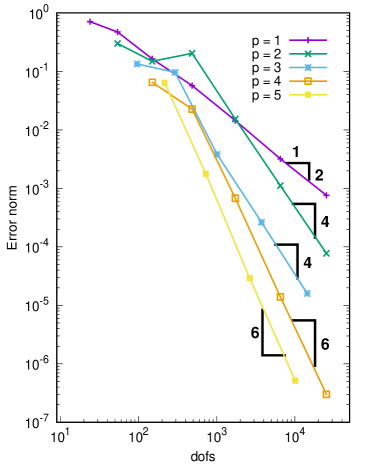
((a)) $\|{\mathbf{u}-\mathbf{u}^{h}}\|_{L^{2}(\Omega)}$.

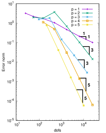
((b)) $\|{\mathbf{u}-\mathbf{u}^{h}}\|_{H^{1}(\Omega)}$.

Figure 2: Asymptotic convergence results.

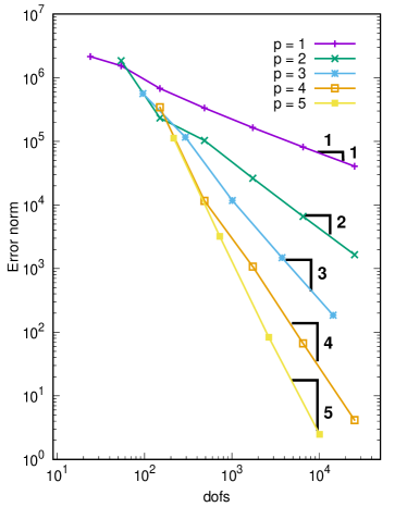
((a)) $\|{(\mathbf{u}-\mathbf{u}^{h},\boldsymbol{\sigma}-\boldsymbol{\sigma}^{h})}\|_{U(\Omega)}$.

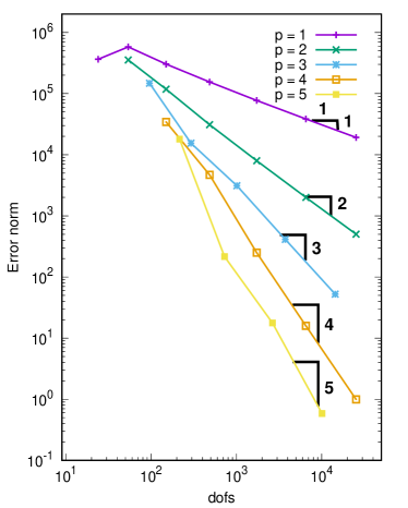
((b)) $\|{(\mathbf{u}-\mathbf{u}^{h},\boldsymbol{\sigma}-\boldsymbol{\sigma}^{h})}\|_{\text{B}}$.

Figure 3: Asymptotic convergence results.

This problem was also considered in ²³ for the DPG method and we point out that the convergence rates of the AVS-FE approximations match the presented rates in ²³.

3.2 Comparison with Other FE Methods

To compare the AVS-FE method for nearly incompressible elasticity to other FE methods, we consider a model problem of which the solution is a function of the Poisson’s ratio from ⁴⁶. The exact solution is given in (37), we use the same Young’s modulus as in the preceding example. However, we increase the Poisson’s ratio to $0.49999999$ to make the problem more challenging with a Lamé parameter $\lambda$ of the order $10^{11}$.

$$\begin{array}[]{rl}\displaystyle\mathbf{u}^{ex}(\mathbf{x})=\begin{Bmatrix}\displaystyle u^{ex}_{x}(\mathbf{x})\\ \displaystyle u^{ex}_{y}(\mathbf{x})\\ \end{Bmatrix}=\begin{Bmatrix}\displaystyle\text{sin}(2\pi y)\left[-1+\text{cos}(2\pi x)\right]+\frac{\displaystyle\text{sin}(\pi x)\text{sin}(\pi y)}{1+\lambda}\\ \displaystyle\text{sin}(2\pi x)\left[1-\text{cos}(2\pi y)\right]+\frac{\displaystyle\text{sin}(\pi x)\text{sin}(\pi y)}{1+\lambda}\\ \end{Bmatrix},\end{array}$$ (37)

The methods we consider are the Bubnov-Galerkin (see Chapter 26 in ⁴⁹ for a description of the implementation of this method) and a mixed method of Arnold and Winther ^{50, 7} in addition to the AVS-FE method. For the Bubnov-Galerkin method, we approximate $\mathbf{u}$ using $C^{0}(\Omega)$ linear polynomials. Likewise, for the first-order system least squares method we use linear polynomials for both variables $\mathbf{u}$ and $\boldsymbol{\sigma}$, and in the AVS-FE approximation we use linear polynomials and first order Raviart-Thomas bases for $\mathbf{u}$ and $\boldsymbol{\sigma}$, respectively. In the mixed method, $\mathbf{u}$ is approximated with linear discontinuous polynomials and $\boldsymbol{\sigma}$ with the lowest order Arnold-Winther element (i.e., cubic). The initial mesh we consider is uniform, consisting of 8 triangular elements, and we proceed to perform uniform mesh refinements.

In Figure 4 we compare the convergence history of these three methods in terms of the $L^{2}$, and $H^{1}$ norms (only $L^{2}$ for the mixed method) of the error on $\mathbf{u}-\mathbf{u}^{h}$. The Bubnov-Galerkin method performs well initially, but upon continued mesh refinements becomes unstable, as indicated by the diverging errors. The AVS-FE method does not suffer from these issues, and retains the optimal rates of convergence in both $L^{2}$ and $H^{1}$ norms. The increasing errors of the Bubnov-Galerkin FE method is likely due to ill conditioning of the resulting stiffness matrices. By lowering the Poisson ratio this effect of ill conditioning is negated, as expected. Thereby limiting the applicability of the Bubnov-Galerkin FE method for nearly incompressible materials. Finally, the mixed method of Arnold and Winther, remains stable as expected. However, in the last two refinements, the rate of convergence is reduced slightly. We attribute this to ill conditioning as in the Bubnov-Galerkin FE method. This has also been observed and studied by Carstensen et al. in ⁵⁰, where it is noted that for pure Dirichlet boundary conditions the stiffness matrix condition number grows to infinity as $\nu\rightarrow 0.5$ (see Section 3.3 in ⁵⁰) ).

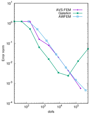
((a)) $\|{\mathbf{u}-\mathbf{u}^{h}}\|_{L^{2}(\Omega)}$.

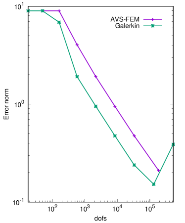
((b)) $\|{\mathbf{u}-\mathbf{u}^{h}}\|_{H^{1}(\Omega)}$.

Figure 4: Comparison between the AVS-FE method, the mixed method of Arnold and Winther, and the Bubnov-Galerkin FE method.

3.3 Adaptive Mesh Refinement

Modern engineering materials often consist of multiple constituents, i.e., composites. Material inclusions often lead to stress concentrations and need to be accurately resolved to ensure confidence in the engineering design. Resolution of such features is typically achieved by carefully constructed FE meshes which requires a significant effort from analysts, or mesh refinements. Until this point, we have presented numerical verifications in which the mesh partitions are uniform and their refinements are uniform as well, since the solutions are known to be rather well behaved, a priori. While these certainly give us confidence in the AVS-FE approximations, the computational cost of uniform mesh refinements becomes very large as $h\rightarrow 0$. To this end, we consider adaptive mesh refinements that are guided by the built-in error indicators (26). As an adaptive strategy, we choose the marking strategy and refinement criteria of Dörfler ⁵¹ using a fixed parameter $\theta=0.5$.

As an example of a simplified composite material we consider a unit square domain with an inclusion in the center at $x=y=0.5$, as shown in Figure 5 The matrix material is nearly incompressible and the inclusion is a stiff material with Young’s modulus several orders of magnitude larger than the bulk material. In Table 2 the properties of the materials are listed. Materials with these properties are, e.g., Silicone based rubber for the matrix and an epoxy based inclusion.

Table 2: Material properties.

Physical property	Young’s Modulus	Poisson’s Ratio.
Matrix	1,500 MPa	0.49
Inclusion	10,000 MPa	0.3

The boundary conditions are as shown in Figure 5 i.e., a surface traction $\mathbf{t}=\{100\text{MPa},0\}^{T}$ on the right side and a fully clamped boundary on a portion of the left side.

Figure 5: Linear elastic problem with inclusion.

Hence, we expect significant concentration of stresses near the inclusion. We employ the error representation function (26) as an a posteriori error estimate. The goal of the adaptive algorithm is then to minimize this error based on its local error indicators.

To establish an initial mesh taking into account the circular geometry with reasonable accuracy, we employ the built-in FEniCS ⁴³ mesh generation functionality. In particular, we use the tool "mshr" to create an inclusion consisting of 250 line segments to accurately represent the circumference of the circle. The initial mesh is shown in Figure 6.

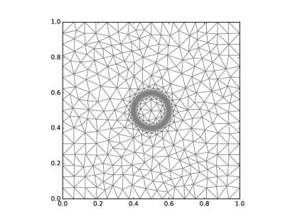
Figure 6: Initial mesh for the inclusion problem.

For the AVS-FE approximations, we consider second order approximations for all variables in both cases of RT and $C^{0}(\Omega)$ stress approximations.

The normal stresses $\sigma_{xx}$ and $\sigma_{yy}$ are presented in Figure 7 where the stresses, as expected, are concentrated near the stiff inclusion. Furthermore, we see in this figure that the stresses perpendicular to the loading, i.e., $\sigma_{yy}$ are dominated by the Poisson effect which is another indication that the AVS-FE approximation of this problem is consistent with the expected physics. As a sanity check, we also note that the far field stresses are equal to the applied surface traction $\mathbf{t}$, see Figure 7(a).

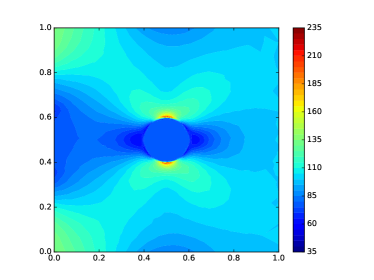
((a)) $\sigma_{xx}^{h}(\mathbf{x})$.

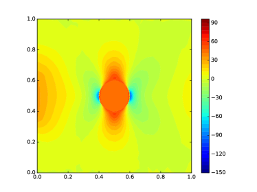
((b)) $\sigma_{yy}^{h}(\mathbf{x})$.

Figure 7: AVS-FE approximate normal stress components (MPa).

The shear stress component $\tau_{xy}$ is shown in Figure 8 along with the adapted mesh after 12 refinements.

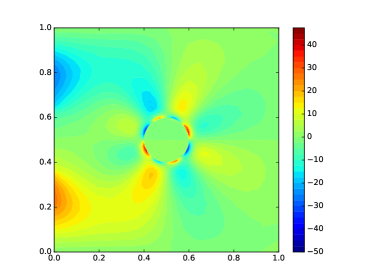
((a)) $\tau_{xx}^{h}(\mathbf{x})$.

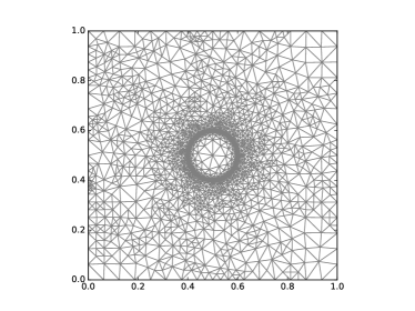
((b)) Final adapted mesh using RT stress approximations.

Figure 8: AVS-FE approximate shear stress component (MPa) and final mesh.

The final adapted mesh shown in figure 8(b) highlights that the built-in error indicators as well as the marking strategy of Dörfler lead to mesh refinements in locations critical to proper resolution of physical features.

Computing these results in the AVS-FE method is straightforward due to its built-in error estimate and discrete stability. Hence, the effort in implementation of the adaptive algorithm is minimal and requires only a FE solver with mesh refinement capabilities. However, it is worth mentioning that the required effort to establish similar results in the Bubnov-Galerkin FE method would be significant. While several a posteriori error estimation techniques exists, the stability issue that arises with the jump in material coefficients will likely require significant efforts in analysis to ensure stability of the error estimation or prohibitively large mesh generation efforts.

Finally, we compare $C^{0}(\Omega)$ and RT stress approximations. The inclusion leads to a stress field that has continuous normal components across the interface between the two materials, whereas the tangential components are discontinuous. While this domain is still convex, we therefore expect that the generally advocated $C^{0}(\Omega)$ stress approximations in the AVS-FE method will be less accurate than the standard mixed FE choice of RT discretization. Thus, as a verification we consider both types of stress approximations in this experiment and measure the difference between the two by the approximate energy norm. To this end, we employ the same adaptive algorithm for the case of $C^{0}(\Omega)$ stresses and in Figure 9, the convergence histories of the approximate error in the energy norm through (26) for both cases are presented. As expected, in this case the RT approximations lead to lower energy norm errors due to the pollution effect of enforcing continuity of tangential stress components for the $C^{0}(\Omega)$ case.

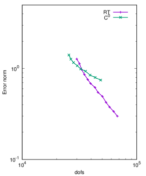
Figure 9: Convergence of the energy norm comparing $C^{0}(\Omega)$ and RT stress approximations computed using the approximate energy norm, see (26).

Finally, in Figure 10 the final adapted mesh for the case of $C^{0}(\Omega)$ stresses are presented. The overly restrictive stress approximations lead to mesh refinements that do not resolve the stress field near the inclusion in the same was as the RT case as evident from comparison of Figures 8(b) and 10. Hence, the $C^{0}(\Omega)$ stress approximations are not applicable for this problem.

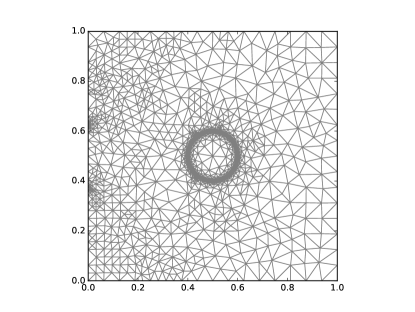
Figure 10: Final adapted mesh using $C^{0}(\Omega)$ stress approximations.

3.4 Engineering Application: Non-Uniform Bending of a 2D Beam

To further illustrate the AVS-FE method in its application to FE analyses of nearly incompressible solids, we present a common engineering application of non-uniform bending of beams. The 2D problem concerns a beam with a length $L=2$m and slenderness ratio $L/H=10$, and consists of a homogeneous linearly elastic isotropic material with a Young’s Modulus equal to that of a nitrile based rubber, i.e., $E=1.5$MPa. The Poisson ratio $\nu$ is chosen such that $\frac{1}{2}-\nu=10^{-9}$ and therefore the material is nearly incompressible. The beam is subject to kinematic constraints along its left edge, where material particles are prohibited from moving in the $x$ direction but free to move in the $y$ direction. To eliminate the rigid body translation in the $y$ direction, the bottom left corner point is kept fixed. In terms of loading, the beam is subject to a downward uniform distributed force $q$, of $3.33$N/m as depicted in Figure 11).

Figure 11: Linear elastic beam problem.

For our numerical experiment of the AVS-FE method, we start with an initial uniform mesh of four triangular elements (two elements in the length, versus one in the height) and subsequently conduct uniform $h$-refinements in which each element is partitioned into four new elements. In all computations, we employ quadratic (i.e., $p=2$) $C^{0}$ trial functions for the displacements and second order Raviart-Thomas functions functions for the stress variable. The evolution of the elastic strain energy of the AVS-FE solutions throughout the $h$-refinement process are shown in orange in Figure 12. In comparison, the corresponding results for the classical FE, or Bubnov-Galerkin, method are also shown in this graph in blue. These were established by using the same mesh partitions as for the AVS-FE method but employing the classical $C^{0}$ quadratic Lagrangian trial functions for the displacements and a standard displacement based weak formulation, as is common in classical Bubnov-Galerkin analyses.

Figure 12 shows that, as expected for this level of near incompressibility, the classical FE solutions fail to converge and start to exhibit spurious behavior as $h\longrightarrow 0$ with greatly changing values for the elastic strain energy between successive solutions. The AVS-FE method, on the other hand, maintains numerical stability from the onset and exhibits convergence upon continued uniform mesh refinements. The converged AVS-FE solutions are physically valid, as can be seen in Figure 13, in which contour plots of the distributions of the normal stress $\sigma_{xx}$ (Figure 13(a)) and shear stress $\tau_{xy}$ (Figure 13(b)) are shown of the AVS-FE solution for the mesh consisting of $22\times 11$ elements. Since Raviart-Thomas trial functions have been used to compute the stress variables, minor discontinuities across inter-element edges can be observed, but these attenuate as the mesh is further refined. Hence, the AVS-FE method shows less sensitivity to the nearly incompressible constitutive behavior of the material than the classical FE method.

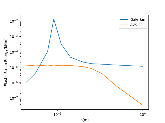
Figure 12: Non-uniform bending of a nearly incompressible beam – elastic strain energy evolution.

((a)) Normal Stress $\sigma_{xx}$ (kPa).

((b)) Shear stress $\tau_{xy}$ (kPa).

Figure 13: AVS-FE stress distributions of beam in bending with $\frac{1}{2}-\nu=10^{-9}$.

4 Conclusions

We have presented a mixed FE method that results in continuous FE approximations of both the displacement and (normal) stress fields in linear elasticity. In particular, we considered nearly incompressible materials as classical FE methods suffer from loss of discrete stability for such materials. The DPG philosophy of optimal test spaces leads to stable FE approximations without reformulation of the problem using the compliance tensor for the case for the nearly incompressible case. The DPG method we present distinguishes itself from the DPG method by only breaking the test space while keeping the trial space globally confirming. Hence, in the corresponding FE approximation we use classical FE bases such as Lagrange polynomials and Raviart-Thomas functions.

We present a priori error bounds in terms of norms of the numerical approximation errors of both displacement and stress trial variables. These bounds are are all optimal in the sense that the approximation errors converge at rates equal to their underlying interpolating functions. Numerical verifications of the asymptotic convergence properties confirm the established error bound in all appropriate norms. A convergence study comparing our method to existing FE methods, i.e., Bubnov-Galerkin FE method and the mixed FE method of Arnold and Winther ⁷, show that the AVS-FE method is superior for the case of nearly incompressible materials for the presented verification. In the verification presented, the Bubnov-Galerkin FE method suffered from a loss of stability as the mesh was refined, thereby resulting in loss of convergence. The mixed method of Arnold and Winther did not lose stability but for highly refined meshes a reduction in convergence rate was observed. The AVS-FE method did not exhibit these types of behavior, nor have we observed such behavior for other verifications we have performed. We attribute this to the scaling term $h^{2}_{m}$ of the $H^{1}$ seminorm portion of $\|{\cdot}\|_{{V(\mathcal{P}_{h})}}$ (8) as it ensures entries in the resulting stiffness matrix are of similar order of magnitude. However, we cannot rule out such behavior for the AVS-FE method for very fine meshes as this is an issue of numerical linear algebra and not the AVS-FE method. Similar behavior has been observed by Storn in ⁵² for the DPG method, where it is attributed to the inversion of the Gram matrix in the computation of optimal test functions.

By considering a global saddle point form of the AVS-FE method, we establish both approximations of the displacement an stress fields as well as an approximation of an error representation function which measures the global energy error of the AVS-FE approximation. This error representation leads to a posteriori error estimates and error indicators which we employ in a mesh adaptive strategy. We present a numerical verification of a challenging physical application of a composite material where the built-in error indicator is used to drive adaptive mesh refinements to resolve the stress field in the composite.

While successful for the presented composite material, the built-in error indicator is a local indication of the residual of the AVS-FE approximation (see (25)). However, in certain applications, localized solution features may be of higher importance than the global energy error. Hence, goal-oriented error estimates and error indicators based on local quantities of interest ⁵³ can provide alternative mesh refinement strategies. As shown in ³⁷, alternative AVS-FE goal-oriented error estimates are capable of accurately estimating these errors and driving goal-oriented mesh refinements. While we have considered a single AVS-FE weak formulation here (5), as mentioned in Remark 2.2, this is not a unique choice. In ²⁵, multiple weak formulations for linear elasticity are considered for the DPG method, all of which provide slightly different FE approximations. Such investigation for the AVS-FE method and comparison of the DPG and AVS-FE methods for linear elasticity are postponed to future works.

References

- 1 Babuška I, Suri M. Locking effects in the finite element approximation of elasticity problems. Numerische Mathematik 1992; 62(1): 439–463.
- 2 Babuška I, Suri M. On locking and robustness in the finite element method. SIAM Journal on Numerical Analysis 1992; 29(5): 1261–1293.
- 3 Oden JT, Reddy JN. An introduction to the mathematical theory of finite elements. Dover Publications . 2012.
- 4 Phillips PJ, Wheeler MF. Overcoming the problem of locking in linear elasticity and poroelasticity: an heuristic approach. Computational Geosciences 2009; 13(1): 5–12.
- 5 Brezzi F, Fortin M. Mixed and Hybrid Finite Element Methods. 15. Springer-Verlag . 1991.
- 6 Falk RS. Finite element methods for linear elasticity. In: Springer. 2008 (pp. 159–194).
- 7 Arnold DN, Winther R. Mixed finite elements for elasticity. Numerische Mathematik 2002; 92(3): 401–419.
- 8 Arnold DN, Winther R. Nonconforming mixed elements for elasticity. Mathematical models and methods in applied sciences 2003; 13(03): 295–307.
- 9 Gopalakrishnan J, Guzmán J. A second elasticity element using the matrix bubble. IMA Journal of Numerical Analysis 2012; 32(1): 352–372.
- 10 Quinelato TO, Loula AF, Correa MR, Arbogast T. Full H (div)-approximation of linear elasticity on quadrilateral meshes based on ABF finite elements. Computer Methods in Applied Mechanics and Engineering 2019; 347: 120–142.
- 11 Ambartsumyan I, Khattatov E, Nordbotten JM, Yotov I. A multipoint stress mixed finite element method for elasticity on simplicial grids. SIAM Journal on Numerical Analysis 2020; 58(1): 630–656.
- 12 Chiumenti M, Valverde Q, De Saracibar CA, Cervera M. A stabilized formulation for incompressible elasticity using linear displacement and pressure interpolations. Computer methods in applied mechanics and engineering 2002; 191(46): 5253–5264.
- 13 Nakshatrala K, Masud A, Hjelmstad K. On finite element formulations for nearly incompressible linear elasticity. Computational Mechanics 2008; 41(4): 547–561.
- 14 Masud A, Xia K. A stabilized mixed finite element method for nearly incompressible elasticity. Journal of Applied Mechanics, Transactions ASME 2005; 72(5): 711–720.
- 15 Malkus DS, Hughes TJ. Mixed finite element methods—reduced and selective integration techniques: a unification of concepts. Computer Methods in Applied Mechanics and Engineering 1978; 15(1): 63–81.
- 16 Hansbo P, Larson MG. Discontinuous Galerkin methods for incompressible and nearly incompressible elasticity by Nitsche’s method. Computer methods in applied mechanics and engineering 2002; 191(17-18): 1895–1908.
- 17 Liu R, Wheeler M, Dawson C. A three-dimensional nodal-based implementation of a family of discontinuous Galerkin methods for elasticity problems. Computers & structures 2009; 87(3-4): 141–150.
- 18 Bochev PB, Gunzburger MD. Least-Squares Finite Element Methods. 166. Springer Science & Business Media . 2009.
- 19 Demkowicz L, Gopalakrishnan J. A Class of Discontinuous Petrov-Galerkin Methods. II. Optimal Test Functions. Numerical Methods for Partial Differential Equations 2011; 27(1): 70-105.
- 20 Cai Z, Starke G. First-order system least squares for the stress-displacement formulation: linear elasticity. SIAM journal on numerical analysis 2003; 41(2): 715–730.
- 21 Cai Z, Korsawe J, Starke G. An adaptive least squares mixed finite element method for the stress-displacement formulation of linear elasticity. Numerical Methods for Partial Differential Equations: An International Journal 2005; 21(1): 132–148.
- 22 Gopalakrishnan J, Qiu W. An analysis of the practical DPG method. Mathematics of Computation 2014; 83(286): 537–552.
- 23 Bramwell J, Demkowicz L, Gopalakrishnan J, Qiu W. A locking-free hp DPG method for linear elasticity with symmetric stresses. Numerische Mathematik 2012; 122(4): 671–707.
- 24 Fuentes F, Keith B, Demkowicz L, Le Tallec P. Coupled variational formulations of linear elasticity and the DPG methodology. Journal of Computational Physics 2017; 348: 715–731.
- 25 Keith B, Fuentes F, Demkowicz L. The DPG methodology applied to different variational formulations of linear elasticity. Computer Methods in Applied Mechanics and Engineering 2016; 309: 579–609.
- 26 Hughes TJ, Cottrell JA, Bazilevs Y. Isogeometric analysis: CAD, finite elements, NURBS, exact geometry and mesh refinement. Computer methods in applied mechanics and engineering 2005; 194(39-41): 4135–4195.
- 27 Surana KS, Reddy J, Romkes A. Mathematical and Computational Finite Element Framework for Boundary Value and Initial Value Problems. Acta Mechanica Solida Sinica 2010; 23: 12-25.
- 28 Taylor R. Isogeometric analysis of nearly incompressible solids. International Journal for Numerical Methods in Engineering 2011; 87(1-5): 273–288.
- 29 Oswald P. Intergrid transfer operators and multilevel preconditioners for nonconforming discretizations. Applied Numerical Mathematics 1997; 23(1): 139–158.
- 30 Ainsworth M. Robust a posteriori error estimation for nonconforming finite element approximation. SIAM Journal on Numerical Analysis 2005; 42(6): 2320–2341.
- 31 Calo VM, Romkes A, Valseth E. Automatic variationally stable analysis for FE computations: an introduction. In: Springer. 2020 (pp. 19–43).
- 32 Valseth E. Automatic Variationally Stable Analysis for Finite Element Computations. PhD thesis. South Dakota School of Mines and Technology, Rapid City, South Dakota; 2019.
- 33 Girault V, Raviart PA. Finite Element Methods for Navier-Stokes Equations; Theory and Algorithms. In: . 5. Springer-Verlag. 1986.
- 34 Carstensen C, Demkowicz L, Gopalakrishnan J. A Posteriori Error Control for DPG Methods. SIAM Journal on Numerical Analysis 2014; 52(3): 1335-1353.
- 35 Carstensen C, Demkowicz L, Gopalakrishnan J. Breaking spaces and forms for the DPG method and applications including Maxwell equations. Computers & Mathematics with Applications 2016; 72(3): 494–522.
- 36 Babuška I. Error-Bounds for Finite Element Method. Numerische Mathematik 1971; 16: 322-333.
- 37 Valseth E, Romkes A. Goal-oriented error estimation for the automatic variationally stable FE method for convection-dominated diffusion problems. Computers and Mathematics with Applications 2020; 80(12): 3027 - 3043. doi: https://doi.org/10.1016/j.camwa.2020.10.019
- 38 Boffi D, Brezzi F, Fortin M. Mixed finite element methods and applications. 44. Springer . 2013.
- 39 Nagaraj S, Petrides S, Demkowicz LF. Construction of DPG Fortin operators for second order problems. Computers & Mathematics with Applications 2017; 74(8): 1964–1980.
- 40 Demkowicz L, Zanotti P. Construction of DPG Fortin operators revisited. Computers & Mathematics with Applications 2020.
- 41 Salazar J, Mora J, Demkowicz L. Alternative enriched test spaces in the DPG method for singular perturbation problems. Computational Methods in Applied Mathematics 2019; 19(3): 603–630.
- 42 Demkowicz L, Gopalakrishnan J. Discontinuous Petrov-Galerkin (DPG) Method. ICES Report 2015.
- 43 Alnæs MS, Blechta J, Hake J, et al. The FEniCS project version 1.5. Archive of Numerical Software 2015; 3(100): 9–23.
- 44 Babuška I, Suri M. The version of the finite element method with quasiuniform meshes. ESAIM: Mathematical Modelling and Numerical Analysis-Modélisation Mathématique et Analyse Numérique 1987; 21(2): 199–238.
- 45 Rivière B, Wheeler MF, Girault V. Improved energy estimates for interior penalty, constrained and discontinuous Galerkin methods for elliptic problems. Part I. Computational Geosciences 1999; 3(3-4): 337–360.
- 46 Brenner SC. A nonconforming mixed multigrid method for the pure displacement problem in planar linear elasticity. SIAM Journal on Numerical Analysis 1993; 30(1): 116–135.
- 47 Rathgeber F, Ham DA, Mitchell L, et al. Firedrake: automating the finite element method by composing abstractions. ACM Transactions on Mathematical Software (TOMS) 2017; 43(3): 24.
- 48 Amestoy PR, Duff IS, L’Excellent JY, Koster J. A fully asynchronous multifrontal solver using distributed dynamic scheduling. SIAM Journal on Matrix Analysis and Applications 2001; 23(1): 15–41.
- 49 Logg A, Mardal KA, Wells G. Automated solution of differential equations by the finite element method: The FEniCS book. 84. Springer Science & Business Media . 2012.
- 50 Carstensen C, Günther D, Reininghaus J, Thiele J. The Arnold–Winther mixed FEM in linear elasticity. Part I: Implementation and numerical verification. Computer methods in applied mechanics and engineering 2008; 197(33-40): 3014–3023.
- 51 Dörfler W. A convergent adaptive algorithm for Poisson’s equation. SIAM Journal on Numerical Analysis 1996; 33(3): 1106–1124.
- 52 Storn J. On a relation of discontinuous Petrov–Galerkin and least-squares finite element methods. Computers & Mathematics with Applications 2020.
- 53 Prudhomme S, Oden JT. On goal-oriented error estimation for elliptic problems: application to the control of pointwise errors. Computer Methods in Applied Mechanics and Engineering 1999; 176(1-4): 313–331.