Sensitivity Prewarping for Local Surrogate Modeling

Abstract

In the continual effort to improve product quality and decrease operations costs, computational modeling is increasingly being deployed to determine feasibility of product designs or configurations. Surrogate modeling of these computer experiments via local models, which induce sparsity by only considering short range interactions, can tackle huge analyses of complicated input-output relationships. However, narrowing focus to local scale means that global trends must be re-learned over and over again. In this article, we propose a framework for incorporating information from a global sensitivity analysis into the surrogate model as an input rotation and rescaling preprocessing step. We discuss the relationship between several sensitivity analysis methods based on kernel regression before describing how they give rise to a transformation of the input variables. Specifically, we perform an input warping such that the “warped simulator” is equally sensitive to all input directions, freeing local models to focus on local dynamics. Numerical experiments on observational data and benchmark test functions, including a high-dimensional computer simulator from the automotive industry, provide empirical validation.

1 Introduction

As previously unimaginable computing power has become widely available, industrial scientists are increasingly making use of computationally intensive computer programs to simulate complex phenomena that cannot be explained by simple mathematical models and which would be prohibitively expensive to experiment upon physically. These computer experiments have varied business applications, for example: Zhou (2013) describe virtualization of an injection molding process; Montgomery and Truss (2001) explored the strength of automobile components; Crema et al. (2015) developed a computer model to help manage an assemble to order system. Despite the tremendous supply of computational resources provided by increasingly powerful CPUs, the general purpose GPU computing paradigm, and even more specialized hardware such as tensor processing units, the demands of advanced computer models are still sizeable. As such, there is a market for fitting surrogates to computer simulations: flexible statistical models which learn the input-output mapping defined by the simulator of interest, and are ideally suited to serve as a substitute for the same. For detailed review, see Gramacy (2020); Santner et al. (2018); Forrester et al. (2008).

One popular use of computer experiments is to perform sensitivity analysis (e.g., Oakley and O’Hagan, 2004; Marrel et al., 2009; Gramacy et al., 2013; Da Veiga et al., 2009; Gramacy, 2020, Ch. 8.2). This can consist of determining which of the input parameters are most influential, or even whether some latent combination of the inputs is driving the response. Sensitivity analysis for computer experiments must take into account unique characteristics not found in observational data. As in classical design of experiments, the training data inputs can be chosen, which means there is no need to take into account natural correlation between the input variables. Moreover, the design may be selected to maximize information gain or other criteria (Gramacy, 2020, Ch. 6). Further, in the case of deterministic experiments, we observe input-output dynamics exactly, and sometimes may even have derivative information (or can approximate it). Active Subspaces (AS; Constantine, 2015) exploit the knowledge of these gradients to perform linear sensitivity analysis, that is to say, sensitivity analysis which finds “directions”, or linear combinations of inputs, of greatest influence, rather than evaluating individual input variables. In this article, we will not assume knowledge of the gradient, but we will leverage that the target simulator is smooth, such that we can estimate its AS nonparametrically (Othmer et al., 2016; Palar and Shimoyama, 2017, 2018; Wycoff et al., 2021). These methods are closely related to existing gradient-based kernel dimension reduction (Fukumizu and Leng, 2014) techniques from the statistics literature, which we discuss in a unified framework in Section 2.2.

Global Sensitivity Analysis (GSA), beyond being of interest in and of itself, can also be used to perform a transformation to the input space before applying standard modeling methods, a process referred to as premodeling in Li et al. (2005). Sometimes, this can take the form of variable selection, as in using lasso to select variables before fitting a standard linear model (Belloni et al., 2013). Otherwise, the dimension of the space is not changed, but simply our orientation within it, for instance by changing basis to that implied by Principal Components Analysis (PCA). This has been recommended as a preprocessor for “axis-aligned” methods such as generalized additive models (de Souza et al., 2018) and tree-based methods (Rodriguez et al., 2006). And, of course, these approaches can be combined to learn both a rotated and truncated space, as in principal components regression (Hastie et al., 2009).

In this article, we argue that this approach also has much promise as a preprocessor for local surrogate modeling of large-scale computer experiments (e.g., Gramacy and Apley, 2015; Katzfuss et al., 2020). Practically speaking, what we dub “prewarping” influences the local model both directly and indirectly. Directly, because it redefines the definition of distances between points upon which many surrogate models (e.g., those based on Gaussian process regression) rely to compute relevant spatial correlations, and indirectly, as the definition of “local” changes with the metric, thus influencing neighborhood selection. We build on recently proposed linear GSA techniques and show significant improvement compared to directly applying the local methods to the original input space. Intuitively, GSA based preprocessing handles global trends, and frees the local models to better represent nearby information. We formalize this intuition in Section 3.1 by proposing that the relationship between the warped inputs and the outputs be equally sensitive to every input dimension at the global level. We find that this enhances predictive ability on a battery of test functions and datasets.

This prewarping idea may be compared to preconditioning in numerical analysis (Wathen, 2015), where a central problem is the solution of linear systems $\mathbf{A}\mathbf{x}=\mathbf{b}$. Modern solution algorithms are typically iterative, meaning that they operate by improving a given approximate solution $\tilde{\mathbf{x}}$ over the course of many iterations until a measure of error like $||\mathbf{A}\tilde{\mathbf{x}}-\mathbf{b}||$ is acceptable. Numerical analysts have found that oftentimes, by first performing a linear transformation to the input space, they improve the conditioning of the linear system which results in fewer iterations required for a given level of accuracy. Similarly, we propose performing a linear transformation of the input space based on a GSA in the hope that this will result in fewer data requirements for a given level of accuracy, or greater accuracy given data. If a surrogate prior to the linear transformation corresponds to fitting $y_{i}$ versus $\mathbf{x}_{i}$, afterwards the problem becomes $y_{i}$ versus $\mathbf{L}\mathbf{x}_{i}$, where $\mathbf{L}$ is derived from an appropriate GSA.

In particular, given a large collection of simulator inputs $\mathbf{X}$ and outputs $\mathbf{y}$, we propose first conducting a GSA using a Gaussian Process (GP) fit to a (global) manageably-sized subset of the data. We prefer a separable kernel (details in Section 2), learning correlation decay separately along each dimension. The Automatic Relevance Determination (ARD; Neal, 1996; Rasmussen and Williams, 2006, Ch. 5.1) principle holds that those input dimensions with large kernel length-scales are less important, and can be dropped when conducting variable selection. Scaling each input dimension by the reciprocal of the associated length-scale, one possible $\mathbf{L}$, thus imbues the local surrogate with inductive bias reflecting global trends.

PCA is an option that goes beyond re-scaling to linear projection. However, PCA’s emphasis on dispersion means it’s less useful for surrogate modeling, where designs are typically chosen by the practitioner; i.e., no input dispersion to learn beyond that we have ourselves imposed. AS, however, allows for non-axis aligned measures of sensitivity, emitting an $\mathbf{L}$ for the purposes of linear projection, while also accounting for the response. We provide the details of how such sensitivities may be realized through efficient sampling schemes, and how $\mathbf{L}$ may be backed out for the purposes of input warping for downstream local analysis, and ultimately accurate prediction. We privilege AS $\mathbf{L}$ prewarping as well as two axis-by-axis sensitivity analyses, which we show both improve upon simple global and local schemes, however there are certainly other possibilities.

After reviewing relevant background in Section 2, our proposed methodology is detailed in Section 3. Section 4 begins by deploying our method on observational data and low dimensional test functions, before tackling our motivating automotive example, a $124$ dimensional problem with $500{,}000$ observations. Section 5 concludes the article and overviews promising future work.

2 Background and Related Work

We review Gaussian processes before pivoting to gradient sensitivity analysis.

2.1 Gaussian Processes

Rather than specifying a functional form, a GP simply defines covariances between input points via some function of the distance between them. For example:

$$\mathbb{V}\mathrm{ar}\left[y(\mathbf{x}_{i}),y(\mathbf{x}_{j})\right]=\sigma^{2}\exp\left\{\frac{-||\mathbf{x}_{i}-\mathbf{x}_{j}||_{2}^{2}}{2l}\right\},$$ (1)

where the length-scale parameter $l$ controls how quickly correlation decays as the distance between the inputs increases, and the covariance parameter $\sigma$ scales the correlation to turn it into a covariance. Broadly speaking, GP kernels differ firstly in how they calculate distance, and secondly in how that distance is translated into a covariance. Isotropic kernels such as (1) are those for which every input dimension is treated identically in terms of distance calculations, whereas anisotropic kernels are free to violate this. For instance, a tensor-product kernel assigns a different length-scale to each dimension, allowing for correlation to decay at different rates as different parameters are varied. Mathematically, this may be expressed as

$$k(\mathbf{x}_{i},\mathbf{x}_{j}):=\mathbb{V}\mathrm{ar}\left[y(\mathbf{x}_{i}),y(\mathbf{x}_{j})\right]=\sigma^{2}\exp\left\{-\sum_{k=1}^{p}\frac{(x_{i,k}-x_{j,k})^{2}}{2l_{k}}\right\},$$ (2)

and evaluation of this kernel between all pairs is usually stored in a kernel matrix $\mathbf{K}$. Notice that each summand in (2) has a different length-scale $l_{k}$ in the denominator. Since as $l_{k}\to\infty$ the contribution of that dimension to the covariance matrix shrinks to zero, the ARD principle (Neal, 1996; Rasmussen and Williams, 2006, Ch. 5.1) argues that dimensions with large length-scales can be ignored. However, technically speaking, there is no guarantee that variable importance decreases monotonically with respect to its length-scale, see (Lin and Joseph, 2020, Section 4.1) and (Wycoff et al., 2021, Section 3.2) for counterexamples. Operating somewhat along this principle, Sun et al. (2019) and Katzfuss et al. (2020) scale input dimensions according to the inverse of their length-scale before fitting models which involve finding local neighborhoods. This approach will form one of our baselines in Section 3.1.

Inference in a GP is typically conducted in a Bayesian manner. Training data, comprising observations $y(\mathbf{X})$ are collected at certain input locations $\mathbf{X}$ and conditioned on, yielding a posterior GP with modified mean and covariance functions. These latter apply at any desired point $\mathbf{x}_{n+1}$ through textbook multivariate Gaussian conditioning:

$$y(\tilde{\mathbf{x}})|\mathbf{y}(\mathbf{X}) \sim N(\mu_{n+1},\Sigma_{n+1}) \mu_{n+1} =\beta_{0}+k(\tilde{\mathbf{x}},\mathbf{X})k(\mathbf{X},\mathbf{X})^{-1}(\mathbf{y}-\beta_{0}\mathbf{1})$$ (3)

$$\Sigma_{n+1} =k(\tilde{\mathbf{x}},\tilde{\mathbf{x}})-k(\tilde{\mathbf{x}},\mathbf{X})k(\mathbf{X},\mathbf{X})^{-1}k(\mathbf{X},\tilde{\mathbf{x}}).$$

The most straightforward way to obtain these quantities involves calculating the Cholesky decomposition of the kernel matrix $k(\mathbf{X},\mathbf{X})$, an operation which scales cubically with the number of training locations, $n$, and is computationally intractable when $n$ is in the low thousands. Much recent work seeks to circumvent this bottleneck.

2.1.1 Scaling Gaussian Processes to Many Observations

Exploiting the fact that an input point will generally only have high correlation with its neighbors, Local Approximate Gaussian Processes (laGP; Gramacy and Apley, 2015; Gramacy, 2020, Ch. 9.3), involve constructing a small model at prediction time, incorporating only training points near where a prediction is desired. These points may be selected via Nearest Neighbors (NN) or more sophisticated criteria. The Vecchia approximation (Vecchia, 1992) also exploits neighborhood structure, but this is used to build a partitioned likelihood. Originally introduced for geospatial data, the Vecchia approximation is most comfortable in low dimensional input spaces, which has motivated a thread of research to adapt it to higher dimensional problems such as surrogate modeling (Katzfuss et al., 2020). That these models select a neighborhood set on the basis of inter-point distances means that proper prewarping could not only give the model a better perspective of distances within the set of local points itself, but also lead to a better set of local points.

Another class of approaches involves choosing a kernel which represents the inner product of a finite-dimensional yet sufficiently rich feature space. Then, the kernel matrix $K$ has a rank bounded by the dimension of the feature space, and can be decomposed efficiently using Woodbury identities. This is the thrust of Fixed Rank Kriging (Cressie and Johannesson, 2008). Or, instead of calculating the kernel on all $\mathcal{O}(n^{2})$ training pairs, the inner product may be calculated through a smaller set of reference locations, knots, or so-called Inducing Points (Smola and Bartlett, 2001; Snelson and Ghahramani, 2006; Rasmussen and Williams, 2006, Ch. 8).

The concern with large datasets may seem somewhat antithetical to the idea that each observation was obtained at great computational cost and should be optimally exploited, but there’s no other choice in high dimension. Consequently, the adaptation of kernel-based surrogates to high dimensional problems is an area of active research.

2.1.2 Scaling Gaussian processes to High Dimension

GP modeling in high dimension requires large designs to accurately capture signal. However, if we assume that the intrinsic dimension of the function is lower than the nominal input dimension, we may be able to get away with a smaller training dataset if a mapping can be learned into this reduced space. Consequently, many approaches for deploying GP as surrogates in high input dimension settings involve built-in (usually linear) dimension reduction. Perhaps the most straightforward mechanism involves random projection, as exemplified by Random Embeddings Bayesian Optimization (Wang et al., 2016, REMBO), and expanded upon in Binois et al. (2015).

Other options include learning projection matrices before fitting a GP on the reduced space. In the special case of a one-dimensional reduced space, Bayesian inference via Markov-Chain Monte Carlo has been proposed to learn the low dimensional subspace for both observational data (Choi et al., 2011) as well as for computer emulators (Gramacy and Lian, 2012) via Single-Index Models. Djolonga et al. (2013) combine finite differencing in random directions with low rank matrix recovery to discover the projection matrix. Garnett et al. (2014) give this approach a Bayesian treatment, even proposing an adaptive sampling algorithm to sequentially select informative design points. Where finite differencing is appropriate, Constantine et al. (2014) propose to deploy adaptive sampling for selecting the low dimensional projection, and also discuss a heuristic for selecting kernel length-scale parameters on the reduced space.

Instead of defining the GP on a low dimensional space, we could split up the dimensions of the input space and define a model on each one. For instance, Durrande et al. (2012); Duvenaud et al. (2011) propose Additive GPs, where the response is modeled as a sum of stochastic processes defined individually for each main effect. The sum can be expanded to include stochastic processes of any interaction level, as detailed in Durrande et al. (2013), or scalar transformations of the response, as in Lin and Joseph (2020). Delbridge et al. (2020) lies at the intersection of random projection and additive kernels: several random projections are combined additively.

2.2 Gradient-Based Sensitivity Analysis

If derivatives of the simulator are available with respect to input parameters, a natural way to define importance of the inputs is via the magnitude of $\frac{\partial f(\mathbf{x})}{\partial x_{i}}$ since this quantity tells us how much the output changes as input variable $i$ is perturbed, assuming the input scales are comparable. Global sensitivity analysis proceeds by defining some method of aggregating such averaging as proposed by Sobol and Gersham (1995), who used $\mathbb{E}\{(\frac{\partial f(\mathbf{x})}{\partial x_{i}})^{2}\}$, estimated via Finite Differencing, as a measure of variable importance for screening purposes. De Lozzo and Marrel (2016) describe a GP based estimator for this quantity. But we are interested in directions of importance, which may be defined by those with large average directional derivatives.

Functions varying only in certain directions are called Ridge Functions, and thus have the form $f(\mathbf{x})=g(\mathbf{A}\mathbf{x})$, where $\mathbf{A}\in\mathbb{R}^{r\times p}$, $g$ is any function on $\mathbb{R}^{r}$, and $r<p$. As a modeling device, ridge functions have inspired a number of nonlinear statistical predictors, including projection pursuit (Friedman and Stuetzle, 1981). In the ridge function framework, dimension reduction is assumed to be linear, but the actual function on the low dimensional space need not be. The left panel of Figure 1 shows the ridge function $f(x)=\sin(x+y)\cos(x+y)e^{-\frac{x+y}{10}}$. Eponymous ridges are visible as constant diagonal bands in the heat plot. Here, $\mathbf{A}=[1\hskip 5.0pt1]$, and $g(z)=\sin(z)\cos(z)e^{-\frac{z}{10}}$. Note, however, that ridge functions cannot exhibit “curvy” ridges, as in the right panel. From the ridge function perspective, the right image represents a two dimensional function, even if it depends only the one dimensional quantity $\sqrt{x^{2}+y^{2}}$.

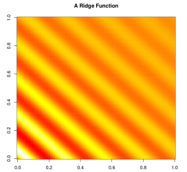
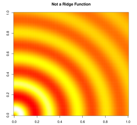
Figure 1: Heat plots of left: $f(z)=\sin(z)\cos(z)e^{-\frac{z}{10}}$, with $z=x+y$; and right: $z=\sqrt{x^{2}+y^{2}}$.

The Active Subspace method (AS; Constantine, 2015) provides a way to view functions as being “almost” ridge functions. This analysis considers the expected gradient outer product matrix with respect to some measure $\nu$:

$$\mathbf{C}=\mathbb{E}_{\nu}\left[\nabla f\nabla f^{\top}\right]=\int\nabla f\nabla f^{\top}\ d\nu\,.$$ (4)

Functions are said to have an AS when they change mostly rather than uniquely along a small set of directions, formalized in the sense that $\mathbf{C}$ has a gap in its eigenvalues. The eigenspace associated with the eigenvalues that make the cut are those directions in which large gradients are “often” pointed, relative to the measure $\nu$.

In this article, the measure with respect to which the AS is defined will either be the Lebesgue measure $\nu_{l}$ or the sample probability measure $\nu_{s}$, which is given by $\nu_{s}(\mathcal{A})=\frac{1}{n}$ if $\mathcal{A}=\{\mathbf{x}_{i}\}$ for any sample point $\mathbf{x}_{i}$ (such that taking the expectation of some quantity with respect to this measure is simply the average of that quantity observed at the sampling locations). We use $\nu$ to denote a generic probability measure.

Readers familiar with techniques such as PCA that analyze the spectrum of the covariance matrix might expect us instead to be interested in

$$\mathbb{E}_{\nu}\left[(\nabla f-\mathbb{E}_{\nu}\left[\nabla f\right])(\nabla f-\mathbb{E}_{\nu}\left[\nabla f\right])^{\top}\right]=\mathbb{E}_{\nu}\left[\nabla f\nabla f^{\top}\right]-\mathbb{E}_{\nu}\left[\nabla f\right]\mathbb{E}_{\nu}\left[\nabla f\right]^{\top},$$

the only difference being that the mean gradient is subtracted prior to the outer product. However, in the case of analyzing gradients rather than data points, the average gradient contains useful information about the function. This is to the extent that Lee (2019) even proposes adding the $\mathbb{E}_{\nu}\left[\nabla f\right]\mathbb{E}_{\nu}\left[\nabla f\right]^{\top}$ term above rather than subtracting it to enhance the influence of that direction.

Analytically computing the integral defining $\mathbf{C}$ is not possible for a general blackbox $f$. However, if the gradient may be evaluated at arbitrary input locations, a Monte Carlo estimator may be formed by first sampling $B$ many vectors $\mathbf{x}_{i}\sim\nu$, and then computing $\frac{1}{B}\sum_{i\in\{1,\ldots,B\}}(\nabla f)(\mathbf{x}_{i})(\nabla f)(\mathbf{x}_{i})^{\top}$. As with the axis-aligned sensitivities, we can of course use finite-difference approximations; Constantine (2015) analyzes the effect of numerical error in this step on the quality of the overall estimate of $\mathbf{C}$.

In situations where finite differencing is not appropriate, the derivative may again be estimated via nonparametric methods (Othmer et al., 2016; Palar and Shimoyama, 2017, 2018). Given a GP posterior with constant prior mean $\beta_{0}$ on $f$, a natural way to estimate $\mathbf{C}$ is to use the posterior mean of the integral quantity it is defined by (Eq. 4), which is now a random variable as we are conducting Bayesian inference. Assuming a sufficiently smooth kernel function, the gradient vector at any point $\mathbf{x}^{*}$ has a multivariate Gaussian posterior $\nabla f(\mathbf{x}^{*})\sim N(\mu_{\nabla},\Sigma_{\nabla})$, where

$$\mu_{\nabla} =\mathbf{K}_{[\nabla,X]}\mathbf{K}_{[X,X]}^{-1}(\mathbf{y}-\beta_{0})\,,$$

$$\mbox{and }\quad\Sigma_{\nabla} =K_{[\nabla,\nabla]}-K_{[\nabla,X]}\mathbf{K}_{[X,X]}^{-1}K_{[X,\nabla]}\,.$$

Above, $\mathbf{K}_{[\nabla,X]}$ represents the cross-covariance matrix between the gradient at $\mathbf{x}^{*}$ and the observed outputs $\mathbf{y}$, $\mathbf{K}_{[X,X]}$ that between the outputs $\mathbf{y}$ at each training location, and $\mathbf{K}_{[\nabla,\nabla]}$ represents the prior covariance matrix of the gradient vector. These quantities are easily derived in terms of derivatives of the kernel function $k$ (Rasmussen and Williams, 2006, Ch. 9), and was used as early as Morris et al. (1993) to exploit observed derivative information to improve a computer experiment response surface. We will use these facts to simplify the desired expectation:

$$\mathbb{E}_{f}\left[\mathbf{C}_{\nu}|\mathbf{y}\right] =\mathbb{E}_{f}\left[\mathbb{E}_{\mathbf{x}\sim\nu}\left[\nabla f(\mathbf{x})\nabla f(\mathbf{x})^{\top}\right]|\mathbf{y}\right]$$

$$=\mathbb{E}_{\mathbf{x}\sim\nu}\left[\mathbb{E}_{f}\left[\nabla f(\mathbf{x})\nabla f(\mathbf{x})^{\top}|\mathbf{y}\right]\right]=\mathbb{E}_{\mathbf{x}\sim\nu}\left[\Sigma_{\nabla}(\mathbf{x})+\mu_{\nabla}(\mathbf{x})\mu_{\nabla}(\mathbf{x})^{\top}\right]\,.$$

For general $\nu$, this expression may be evaluated via Monte Carlo. Wycoff et al. (2021) provided closed forms for when $\nu$ is the Lebesgue measure on $[0,1]^{p}$ (denoted $\nu_{l}$) and $k$ is Gaussian (1–2) or Matérn with smoothness $\frac{3}{2}$ or $\frac{5}{2}$. The quantities above depend on the choice of kernel hyperparameters, which must be estimated. We prefer maximizing the marginal likelihood, but other options work (Fukumizu and Leng, 2014).

The quantity $\mathbf{C}$ was studied for observational data as early as Samarov (1993). Kernel based estimates were proposed by Fukumizu and Leng (2014) with respect to the sample measure $\nu_{s}$, and deployed by Liu and Guillas (2017) to reduce the dimension of a tsunami simulator. Authors have also considered second order derivatives. Li (1992) proposes looking at Hessian eigen-decompositions in Principal Hessian Directions as well as a method to estimate the Hessian itself using Stein’s Lemma, effectively calculating the cross-covariance between the response and the outer product of the input vector. For more on GSA, see Iooss and Lemaître (2015).

3 Methodology

We first discuss how to turn a sensitivity analysis into an input warping before discussing how to fit local models in the warped space.

3.1 Warping

Here we propose the heuristic of using the warping such that running the sensitivity analysis again afterwards would result in all directions being equally important. In the case of ARD, this would amount to conducting a warping such that the optimal length-scales are all equal to 1, while in the case of AS, $\mathbf{C}=\mathbf{I}$. In both of these cases the transformation is linear, and thus can be represented by a matrix $\mathbf{L}$. The matrix $\mathbf{L}$ should premultiply each design point $\mathbf{z}_{i}=\mathbf{L}\mathbf{x}_{i}$, which looks like $\mathbf{Z}=\mathbf{X}\mathbf{L}^{\top}$ when the design points are stacked in the canonical design matrix $\mathbf{X}\in\mathbb{R}^{n\times p}$. This process may be seen as decomposing the black-box $f$ into two parts: a linear transformation $\mathbf{L}$ and a nonlinear function $g$. Here, $g$ is the function upon which we are actually doing regression when we fit $\mathbf{y}$ to $\mathbf{Z}$.

3.1.1 Bandwidth and Range Scaling

When using the separable Gaussian kernel (Eq. 2), a length-scale of $l_{k}$ for input variable $k$ living in $[0,1]$ is equivalent to using a length-scale of $l_{k}=1$ and a domain of $\left[0,\frac{1}{\sqrt{l_{k}}}\right]$. Therefore, scaling each input dimension by the root of its estimated length-scale would achieve our desired result. This is because fitting a GP to the scaled input-output relationship would result in length-scale estimates equal to 1.

Algorithm 1 Bandwidth Scaling

Given: Data $\mathbf{X},\mathbf{y}$, Bags $B$, Bag size nsub, Sample Size $n$,

1:for $b\in\{1,\ldots,B\}$ do

2:     $\mathcal{I}\sim\textrm{Cat}\{1,\ldots,N\}$$\triangleright$ Subsampling

3:     $\hat{\boldsymbol{\theta}}_{b}\leftarrow\underset{\theta}{\textrm{argmin}}\,\mathcal{L}_{GP}(\mathbf{y}_{\mathcal{I}}|\theta)$$\triangleright$ Optimize GP Likelihood wrt $\boldsymbol{\theta}$

4:end for

5:$\hat{\boldsymbol{\theta}}\leftarrow\frac{1}{B}\sum_{\mathcal{B}}\hat{\boldsymbol{\theta}}_{\mathcal{B}}$

6:$\mathbf{L}\leftarrow\textrm{diag}(\hat{\boldsymbol{\theta}})$$\triangleright$ Place Estimates in a Diagonal Matrix

7:$\mathbf{Z}\leftarrow\mathbf{X}\mathbf{L}^{\top}$

Since we are just scaling the input space, $\mathbf{L}$ will be a diagonal matrix with nonzero elements given by the inverse root of the length-scales: $\mathbf{L}_{\mathrm{ARD}}=\mathrm{Diag}\left(\frac{1}{\sqrt{l_{1}}},\frac{1}{\sqrt{l_{2}}},\cdots,\frac{1}{\sqrt{l_{p}}}\right)$. In Gramacy (2020) and Cole et al. (2021) this is treated as a preprocessing step, performed once before deployment within local models, while in Katzfuss et al. (2020) this scaling is iteratively updated as the marginal likelihood is optimized and length-scale estimates change. Cole et al. attributed the idea to Derek Bingham, who called it “stretching and compressing”.

Other approaches of input variable sensitivity could be considered in developing transformations. As recommended by an anonymous reviewer, we will consider another measure of sensitivity to be the range of the GP posterior surface fit to data projected onto a given axis. In particular, to determine the range sensitivity of variable $i$, we first fit a one dimensional GP regression on $\mathbf{X}_{i}$ vs $\mathbf{y}$. Then, the sensitivity is defined as the range of the posterior surface of that GP, that is to say, as $\underset{x_{1},x_{2}\in[0,1]}{\max}|\hat{f}(x_{1})-\hat{f}(x_{2})|$ where $\hat{f}$ is the posterior predictive mean. This is a nonconvex optimization problem which we solve approximately by initializing $x_{1}$ and $x_{2}$ to be the i’th coordinates of those design points corresponding to the largest and smallest observed $y$ values and then applying a quasi-Newton method (L-BFGS-B) refinement.

3.1.2 Active Subspace Rotation

In the case of a known AS matrix $\mathbf{C}$, the transformation $\mathbf{L}$ which satisfies our desire to “undo” the sensitivity analysis is given by $\mathbf{L}=\Lambda^{1/2}\mathbf{U}^{\top}$, where $\mathbf{U}\in\mathbb{R}^{p\times p}$ is the matrix with columns giving the eigenvectors of $\mathbf{C}$ and $\Lambda^{1/2}$ a diagonal matrix containing the square root of the eigenvalues. To how that this warping satisfies our heuristic, recall that $f(\mathbf{x})=g(\mathbf{L}\mathbf{x})$, and let $\nu_{\mathbf{z}}$ be the measure implied on $\mathbf{z}:=\mathbf{L}\mathbf{x}$ by $\nu$.

$$\mathbb{E}_{\nu}\left[\nabla_{x}f(\mathbf{x})\nabla_{x}f(\mathbf{x})^{\top}\right]=\mathbb{E}_{\nu}\left[\nabla_{x}g(\mathbf{L}\mathbf{x})\nabla_{x}g(\mathbf{L}\mathbf{x})^{\top}\right]$$

$$\iff\mathbb{E}_{\nu}\left[\nabla_{x}f(\mathbf{x})\nabla_{x}f(\mathbf{x})^{\top}\right]=\mathbb{E}_{\nu}\left[\mathbf{L}^{\top}(\nabla_{\mathbf{L}x}g(\mathbf{L}\mathbf{x}))(\nabla_{\mathbf{L}x}g(\mathbf{L}\mathbf{x}))^{\top}\mathbf{L}\right]$$

$$\iff\mathbb{E}_{\nu}\left[\nabla_{x}f(\mathbf{x})\nabla_{x}f(\mathbf{x})^{\top}\right]=\mathbf{L}^{\top}\mathbb{E}_{\nu}\left[\nabla_{\mathbf{L}x}g(\mathbf{L}\mathbf{x})\nabla_{\mathbf{L}x}g(\mathbf{L}\mathbf{x})^{\top}\right]\mathbf{L}$$

$$\iff\mathbf{U}\Lambda\mathbf{U}^{\top}=\mathbf{U}\Lambda^{\frac{2}{2}}\mathbb{E}_{\nu}\left[\nabla_{\mathbf{L}x}g(\mathbf{L}\mathbf{x})\nabla_{\mathbf{L}x}g(\mathbf{L}\mathbf{x})^{\top}\right]\Lambda^{\frac{1}{2}}\mathbf{U}^{\top}$$

$$\iff\textbf{I}=\mathbb{E}_{\nu}\left[\nabla_{\mathbf{L}x}g(\mathbf{L}\mathbf{x})\nabla_{\mathbf{L}x}g(\mathbf{L}\mathbf{x})^{\top}\right],$$

or alternatively $\mathbb{E}_{\nu_{\mathbf{z}}}\left[\nabla_{\mathbf{z}}g(\mathbf{z})\nabla_{\mathbf{z}}g(\mathbf{z})^{\top}\right]=\mathbf{I}$. Consequently, all directions are of equal importance globally, and the local model is freed to concentrate on local information. The decomposition is illustrated in Figure 2, which shows the trajectory from simulator input to simulator output in two different ways.

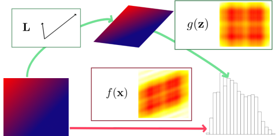
Figure 2: The function $f$ (bottom, red line) with a nontrivial AS maps from $[0,1]^{2}$ to $\mathbb{R}$. It may alternatively be viewed as a linear scaling $\mathbf{L}:[0,1]^{2}\to\mathbb{R}^{2}$, followed by a function $g$ with all directions of equal importance (top, green lines). Before preprocessing, regression is on $f$; afterwards on $g$.

The bottom of the figure shows the standard modeling approach, where the black-box simulator maps directly from the input space to the scalar response in an anisotropic manner. The top shows our proposed decomposition, where first a linear transformation maps the input hypercube into a polytope defined by the sensitivity analysis, and second the now isotropic nonlinear function may be modeled by local predictors. This procedure is delineated in Algorithm 2, which defines a family of warpings parameterized by the measure $\nu$. In this article, we will study the transformations $\mathbf{L}_{l}$, associated with the Lebesgue measure, and $\mathbf{L}_{s}$, associated with the sample measure.

Algorithm 2 Active Subspace Rotation

Given: Data $\mathbf{X},\mathbf{y}$, $\nu\in\{\textrm{Lebesgue},\textrm{Sample}\}$, Bags $B$, Bag size nsub, Sample Size $n$

1:for $b\in\{1,\ldots,B\}$ do$\triangleright$ Subbagging Iteration

2:     $\mathcal{B}\sim\textrm{Cat}(\{1,\ldots,N\},\texttt{nsub})$ $\triangleright$ Subsampling

3:     $\hat{\boldsymbol{\theta}}_{\mathcal{B}}\leftarrow\underset{\theta}{\textrm{argmin}}\,\mathcal{L}_{GP}(\mathbf{y}_{\mathcal{B}},\mathbf{X}_{\mathcal{B}}|\theta)$ $\triangleright$ Optimize GP Likelihood wrt $\boldsymbol{\theta}$

4:     $\hat{\mathbf{C}}_{\mathcal{B}}\leftarrow\mathbb{E}_{\nu}\left[\nabla f(\mathbf{x})\nabla f(\mathbf{x})^{\top}|\mathbf{y}_{\mathcal{B}}\right]$ $\triangleright$ Subset estimate of $\mathbf{C}$

5:end for

6:$\hat{\mathbf{C}}\leftarrow\frac{1}{B}\sum_{\mathcal{B}}\hat{\mathbf{C}}_{\mathcal{B}}$

7:$\mathbf{U},\boldsymbol{\Lambda}\leftarrow\texttt{eigendecomp}(\hat{\mathbf{C}})$

8:$\mathbf{L}\leftarrow\boldsymbol{\Lambda}^{\frac{1}{2}}\mathbf{U}^{\top}$

9:$\mathbf{Z}\leftarrow\mathbf{X}\mathbf{L}^{\top}$

3.1.3 Truncation

Once a transformation $\mathbf{L}$ is calculated, we may additionally select a truncation dimension, creating another, more parsimonious class of options for the warping. Determining the appropriate amount of such truncation depends on what local predictor is to be applied downstream, on the warped (and lower dimensional) inputs. We follow the approach outlined by Fukumizu and Leng (2014), which is actually designed to estimate kernel hyperparameters but it is easily adapted to any low-dimensional parameter, like model complexity. Our pseudo-code in that setting is provided in Algorithm 3. Notice that the method involves NN, however this is just one of many possible downstream models, a discussion we shall table for the moment. We take the same approach to truncation regardless of which GSA method gave rise to $\mathbf{L}$. In particular, NN is applied to each candidate dimension, and the sum of squared residuals computed. Rather than simply choosing that dimension which minimized error magnitude, we found that optimizing the Bayesian Information Criterion (BIC) was superior. In calculating BIC, we treated the dimension of the NN model as the number of parameters it had and endowed it with a Gaussian error structure.

Algorithm 3 Dimension Selection

Given: Rotated Design Matrix $\mathbf{Z}$, search interval [MIND, MAXD].

1:for $r^{*}\in\{\texttt{MIND},\ldots,\texttt{MAXD}\}$ do

2:     $\mathbf{Z}_{r^{*}}\leftarrow\mathbf{Z}[,1:r^{*}]$

3:     $\texttt{mse}[r^{*}]\leftarrow\texttt{mean}(\texttt{resid}(\texttt{KNN}(\mathbf{Z}_{r^{*}},\mathbf{y}))\texttt{\textasciicircum 2})$ $\triangleright$ $\kappa$-Nearest Neighbors

4:     $\texttt{bic}[r^{*}]\leftarrow n\log(\texttt{mse}[r^{*}])+r^{*}\log(n)$

5:end for

6:$r\leftarrow\underset{\texttt{MIND}\leq r^{*}\leq\texttt{MAXD}}{\textrm{argmin}}\texttt{bic}[r^{*}]$

In our experiments (Section 4), all of our local models use the same truncated dimension size $r$ selected by Algorithm 3. Other approaches still are certainly possible. For instance, Constantine (2015) suggests manual examination of $\mathbf{C}$’s spectrum for a gap, though such human intervention may be at odds with the otherwise hands-off, automated approach implied by the surrogate modeling context.

3.1.4 Scaling Up

GP-based estimates of the active subspace carry the GP’s computational burdens, and are limited to comparatively small datasets, just as the GP itself is. We mitigate this via a subbagging approach (Breiman, 1996; Zhao et al., 2018). Given a subbag size $n_{B}<n$ and a number of subbags $B$, we simply sample $n_{B}$ many datapoints at random from our input-output pairs before fitting a GP and developing an estimate of $\mathbf{C}$ based on those data alone. This is repeated $B$ times, and each estimated $\mathbf{C}_{b}$ is combined via averaging to form our estimator $\frac{1}{B}\sum_{b=1}^{B}\mathbf{C}_{b}$. Since we are executing the cubic cost GP operations not on $n$ data but on $n_{B}$ data, the overall computational expense is significantly less on our applications despite the fact that the procedure must be repeated several times. Furthermore, this is an embarrassingly parallel task. Of course, this comes at the cost of estimation error, and, to our knowledge, the impact of such subsampling on the concentration rate of the estimate of $\mathbf{C}$ is an open question. We find that it works in practice in Section 4.

3.2 Local Modeling

For some regression methods, such as the basic linear model, linear transformations such as those we have described in this section so far would have no nontrivial impact. However, this is certainly not the case for local models, which are influenced in two major ways, namely by altering the partitioning scheme and by changing the default distance metric. Before we see exactly how, we provide an overview of the particular local models we prefer; the Supplementary Material provides further detail.

The simplest of these is NN. To predict at $\tilde{\mathbf{x}}$, NN determines the $k$ closest training locations to $\tilde{\mathbf{x}}$, then averages their responses to obtain a prediction. It is thus affected by the linear warping through a warped definition of “closest”, which thus alters the points which are being averaged for each prediction.

The laGP method also operates by building a prediction set at $\tilde{\mathbf{x}}$. And, just like NN, it begins with some number $\kappa$ of nearest neighbors to $\tilde{\mathbf{x}}$. Next, however, points are added to that set based on how useful they will be for prediction as measured by an acquisition criterion built on a GP. This GP is grown until some pre-specified “max” size. Both the conditioning set(s) (like NN), and the local kernel function are a influenced by the linear pre-warping.

The Vecchia approximation is a related but distinct idea. Unlike NN or laGP, which create local models at prediction time, the Vecchia approximation specifies a single generative story for the data. Each datapoint, rather than being conditioned upon all other training data, is instead conditioned on a cascade of subsets, assumed conditionally independent of all others. This requires the data be ordered, making the assumption that any data point is conditionally independent of all those data that come after it in the order. Since vector data in general have no natural ordering, one is generally imposed by sorting along a given axis or finding an ordering that best encodes input distances (Guinness, 2018). The Vecchia approximation stands to benefit from an improved ordering (and kernel structure) via prewarping.

Illustrating Influence on Neighborhood Selection

We shall now visually explore the effect preprocessing can have on the sets of NN. Specifically, points which are farther from the prediction location along axes with little influence, but closer along axes with much influence, are comparatively favored. Figure 3 illustrates this principle, revisiting the ridge function of Figure 1. In this toy example, we sample $400$ input locations uniformly at random in the 2d input domain, then apply Lebesgue-measure prewarping. The left panel shows the original input space, while the right plot shows the new input space after applying a $\mathbf{L}_{l}$ rotation. The training set (black +’s) and prediction location (white triangle) are the same in both, but the closest points (solid circles) are changed. In each panel, the faded circles give the locations of the solid circles from the other plot. We can see that the response value at the ten nearest neighbors is much closer to the value at the predictive location after the warping (right) than it is before (left).

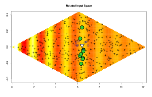
Figure 3: The function $f(x)=\sin(x+y)\cos(x+y)e^{-\frac{x+y}{10}}$ with $x,y$ varying from $-2\pi$ to $2\pi$ rescaled to $[0,1]$, before (left) and after (right) $\mathbf{L}_{\nu_{l}}$ rotation In both panels, the black + represent the training set and solid circles represent the 10 nearest points to an arbitrary prediction location, itself represented by the large white triangle. Faded circles give nearest neighbors from the other plot. Note that the rotated plot is not to scale for ease of viewing.

4 Numerical Experiments

We shall now present results of experiments devised to quantitatively evaluate sensitivity prewarping in predictive exercises. We begin with outlining the comparators and metrics, followed by implementation details, and the actual experiments. R scripts reproducing all figures shown in this document may be found here: https://github.com/NathanWycoff/SensitivityPrewarping

4.1 Implementation details, comparators and metrics

The preprocessing methods will be assessed based on their effect on the performance of downstream local models. As baselines, we entertain GPs fit on random data subsets, which we’ll denote sGP, as well as $k$-NN (KNN), laGP (laGP), and the Vecchia approximation (vecc) on the full, original dataset. Implementations are provided by R packages hetGP (Binois and Gramacy, 2019; Binois et al., 2018), FNN (Beygelzimer et al., 2013), laGP (Gramacy, 2016; Gramacy and Apley, 2015), and GpGp (Guinness, 2018; Guinness et al., 2020), respectively. These will be compared to KNN, laGP and vecc with the four specific prewarping methods proposed in Section 3.1. The Bandwidth Scaling $\mathbf{L}_{\mathrm{ARD}}$ will be denoted by prefix B, Lebesgue-measure prewarping $\mathbf{L}_{l}$ by prefix L, sample-measure prewarping $\mathbf{L}_{s}$ by S, and the range sensitivity prewarping by R. Further, we will consider truncation for all four prewarping techniques which is denoted by a postfix of T.

For each test function, we first generate data using either a random Latin Hypercube Sample (LHS; Stein, 1987) via the R package lhs (Carnell, 2020) for synthetic data, or via uniform random subsampling with existing/observational data, which we then randomly split into train and test sets. Then, we fit the baseline models for $\mathbf{y}$ given $\mathbf{X}$ and calculated their performance. Next, we conducted the sensitivity analyses using $5$ subsamples each of size 1,500 in all experiments, using GP regression to estimate kernel hyperparameters, as well as the nugget term, via MLE (Gramacy and Lee, 2012). Afterwards, we compute the associated transformations to warp each $\mathbf{X}$, yielding each $\mathbf{Z}$, as outlined in Algorithms 1 and 2. Finally, each local model is fit to $\mathbf{Z}$ versus $\mathbf{y}$ for each $\mathbf{Z}$ created by the different transformations, and their performance on each recorded. This process is repeated for 10 Monte Carlo iterations.

In surrogate modeling, quantification of uncertainty is often high priority, so we define performance using not only the Mean Square prediction Error (MSE), but also logarithmic Score (Gneiting and Raftery, 2007). For GP predictors, this is defined as the log likelihood of the response at a prediction location given the predictive mean and variance at that point using our assumption of Gaussianity for the response (Gneiting and Raftery, 2007, Eq. 25). Since NN is typically not deployed in situations where uncertainty quantification is desired, we omit score calculations for it.

While calculation of $\mathbf{C}$ can involve sophisticated machinery, we have endeavored to make its application as simple as possible. With the R package activegp (Wycoff and Binois, 2020; Wycoff et al., 2021) loaded, prewarping is as straightforward as:

  R> Lt <- Lt_GP(X, y, measure = "lebesgue")  ## or measure = "sample"
  R> Z <- X %*% Lt[,1:r]                   ## r is truncated dimension

4.2 Observational Data

We first consider two high dimensional observational datasets. The Communities and Crime dataset (Redmond and Baveja, 2002) combines census and law enforcement statistics from the United States. The task is to predict crime rate per capita given 122 socio-economic indicators measured on 1,994 individuals. The Temperature dataset (Cawley et al., 2006) involves temperature forecasting given the output of a weather model, and consists of 7,117 observations and 106 features.

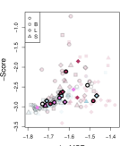
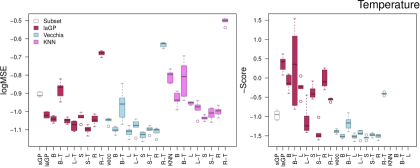
Figure 4: Results on two observational test problems. Left and Center: the $y$-axis gives either $\log_{10}$ MSE or negative Score (smaller is better). The letter before the name, B, L and S represents the transformation used for prewarping (if there is one); T denotes truncation. Bold names indicate prewarping. Models that failed to fit are left blank. Right: logMSE vs -Score for each run; faded icons indicated individual run while solid icons give group medians. Circles indicate no prewarping, solid borders indicate no truncation.

The performance of the competing methods is given in Figure 4. We find that truncation is helpful for high dimensional problems, particularly on the Temperature dataset, and more so for the active subspace rotations than for the axis scaling methods (Bandwidth and Range). We also find that the $\mathbf{L}_{s}$ generally outperforms $\mathbf{L}_{l}$. This is because the observational data are not uniformly distributed, which has two implications. First, since the training set is not uniformly distributed, Sample measure overemphasizes certain parts of the input space compared to Lebesgue. Second, because the test set was formed by random sampling, these same parts of the input space that we have implicitly tuned our $\mathbf{L}$ estimate to are those parts of the input space in which we tend to find testing locations. In other words, there is simply a mismatch between the probability distribution from which the observational data were drawn and that with respect to which $\mathbf{L}_{l}$ is defined. We see that the preprocessing differentiated itself the least on the Communities and Crime problem, potentially because this problem consisted of significantly fewer observations, at around $1{,}000$, making it difficult to estimate the rotation, and leading to high variance.

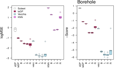
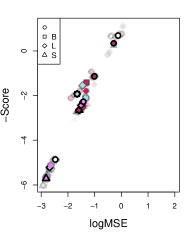
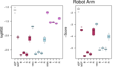
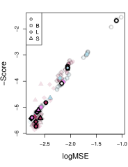
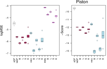
Figure 5: A comparison on common test functions with $n=40{,}000$ runs. See Figure 4 caption.

4.3 Benchmark Test Functions

We next evaluated the proposed methodology on benchmark test functions (Surjanovic and Bingham, 2020) where we found that prewarping increased performance in terms of both MSE and Score. In particular, we ran the competing methods on the Borehole (Harper and Gupta, 1983, $p=8$), Robot Arm (An and Owen, 2001, $p=8$), and Piston (Kenett and Zacks, 1998, $p=7$) functions with a training set size of $40{,}000$ and test set size of $2{,}000$ for each, sampled from a random LHS.

The results, shown in Figure 5, indicate that prewarping can be quite beneficial for local modeling in terms of predictive accuracy. On these low dimensional problems, each method performed similarly regardless of whether truncation was applied, so we have omitted truncation in the results. On all three problems, all forms of prewarping greatly outperform respective baselines. On the Borehole problem the AS based methods $\mathbf{L}_{l}$ and $\mathbf{L}_{s}$ outperform both the baselines and $\mathbf{L}_{\mathrm{ARD}}$ in terms of both MSE and Score. The Range prewarping seems to have a slight edge in MSE and a slight disadvantage in Score. On the Robot Arm function, we find that all prewarping methods are pretty similar, with the sample-measure $\mathbf{L}_{s}$ generally having a slight edge. The Range transformation seems to be at a disadvantage on this problem. Finally, on the Piston problem, prewarping generally leads to a decrease in MSE, though which particular method is ahead depends on the local model considered. Range again does about the same as no prewarping.

4.4 The Jones MOPTA Problem

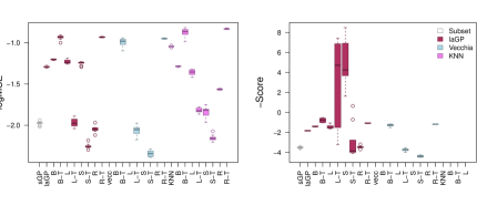
Figure 6: A comparison on the 124d MOPTA function. See Figure 4 caption.

In this section, we study the performance of prewarping on an optimization problem presented by General Motors at the 2008 “Modeling and Optimization: Theory and Applications (MOPTA)” conference (Jones, 2008). The input variables characterize the design of the automobile, such as materials, part gauges, and shape, which determine the results of several crash simulations. The problem is to minimize the mass of the configuration, while observing constraints, such as the durability of the vehicle and the harshness of the crash. This is a constrained optimization problem involving 124 input variables and 68 constraints. While the standard approaches to smooth, high dimensional, constrained optimization are primarily gradient-based, the simulator, a multi-disciplinary effort, does not provide gradients with respect to inputs, and numerical noise means finite differencing approaches are not applicable.

Various authors have proposed sophisticated solutions for this challenging problem, including those based on Bayesian optimization, evolutionary strategies, or both. Regis (2011) proposed fitting a surrogate model to each constraint as well as the objective function to launch a stochastic search for good feasible solutions. Beaucaire et al. (2019) tackled the optimization problem by effectively using an ensemble of surrogates, while Regis (2012) combined surrogate modeling approaches with evolutionary algorithms, and Regis and Wild (2017) combined surrogate modeling with trust region methods. However, this article is concerned with the large data regime, which is generally not the case when conducting Bayesian optimization. To study Jones MOPTA as an emulation problem, we simply treat the sum of the objective and all of the constraints as a black-box function to approximate. This black-box is of interest as such augmented objective functions form the basis of penalty-based approaches to constrained optimization (Nocedal and Wright, 2006).

We sampled $500{,}000$ points uniformly at random in the input space, treating $2{,}000$ as a test set, chosen randomly. We chose not to include vecc fit on the untruncated data as the runtime was too long. As the results in Figure 6 show, in terms of MSE, prewarping without truncation can somewhat improve performance, but throwing in truncation as well results in improvements of an order of magnitude or more using doing AS prewarping ($\mathbf{L}_{s}$ or $\mathbf{L}_{l}$). The exception is S-KNN, which is able to achieve competitive accuracy without truncation. In terms of score, it would appear that prewarping without truncation can result in a significant decrease in performance compared to baseline. Indeed, looking at the scatterplot (Figure 6, right), we see that without truncation, the various local models and prewarpings form a spectrum of solutions trading MSE for Score, whereas the truncated AS prewarped local models significantly outperforms in terms of both. However, this trend is not universal among prewarpings: the Range prewarping performs very well in terms of MSE without truncation, but not with. It seems as though the Range prewarping can offer a good warping of the space, but not one amenable to truncation.

5 Conclusions and Future Work

We introduced Sensitivity Prewarping, a simple-to-deploy framework for local surrogate modeling of computer experiments. Specifically, we proposed the heuristic of warping the space such that a global sensitivity analysis would reveal that all directions are equally important, and showed specific algorithms based on the ARD principle and/or AS to achieve this. By learning directions of global importance, we free each of the local models from individually learning global trends, and instead allow them to focus on their prediction region. Our prewarping effectively defines a new notion of distance which has the dual benefit of improving both neighborhood selection and the value of distance in prediction. We also proposed a subbagging procedure for scaling up inference of the AS as estimated via a GP.

Generally, our numerical experiments revealed that prewarping yields significant benefits in terms of predictive accuracy, as measured by MSE, as well as predictive uncertainty, as measured by Score. We showed how rotations can improve inference on low dimensional test functions, and how truncation can be transformative in high dimensional problems. Given the ease of implementation and the important improvement in predictive accuracy, we submit that this procedure has broad applicability.

We focused on three specific sensitivity analyses and three specific local models, but there is plenty of room for further inquiry. Deploying this framework with nonlinear sensitivity analysis (i.e., that which can measure the importance of nonlinear functions of the inputs) could be fruitful, for instance with Active Manifolds (Bridges et al., 2019). It would also be interesting to study what sensitivity techniques could be expected to perform well when paired with a given local model.

Another area where future work could lend improvements is in large scale estimation of $\mathbf{C}$. In this article, we proposed a subbagging solution, but many other approaches are conceivable. For instance, $\mathbf{C}$ could be computed by using existing approximations to the kernel matrix, such as the Vecchia approximation. An alternative would be to deploy Krylov subspace methods, which have shown great promise in scaling GPs (Wahba et al., 1995; Gibbs and MacKay, 1997; Pleiss et al., 2018; Dong et al., 2017), to develop stochastic algorithms either to estimate the matrix $\mathbf{C}$ itself or its leading eigenspace directly (Golub and Meurant, 2010).

Arguably, the weakest link of this approach is the GP fit in the first stage which produces our estimator of $\mathbf{C}$, required to compute $\mathbf{L}$ in the AS approach. This is because local models can compensate for breaches of our GP assumptions such as stationarity and homoskedasticity, while the global fit cannot. Hence, designing techniques for estimation of $\mathbf{C}$ via more sophisticated models is likely to be a fruitful thread of research. Deep GPs (Damianou and Lawrence, 2013) are a natural next step, and have been recently studied in the context of computer experiments (Sauer et al., 2020). Finally, the simulators we studied in this article all accepted a vector of inputs and returned a scalar response. Extensions to vector-valued, discrete, or functional responses would increase the breadth of problems this framework can take on.

References

- An and Owen (2001) An, J. and A. Owen (2001). Quasi-regression. Journal of Complexity 17(4), 588 – 607.
- Beaucaire et al. (2019) Beaucaire, P., C. Beauthier, and C. Sainvitu (2019). Multi-point infill sampling strategies exploiting multiple surrogate models. In Proceedings of the Genetic and Evolutionary Computation Conference Companion, pp. 1559–1567.
- Belloni et al. (2013) Belloni, A., V. Chernozhukov, and C. Hansen (2013). Inference on Treatment Effects after Selection among High-Dimensional Controls. The Review of Economic Studies 81(2), 608–650.
- Beygelzimer et al. (2013) Beygelzimer, A., S. Kakadet, J. Langford, S. Arya, D. Mount, and S. Li (2013). FNN: Fast Nearest Neighbor Search Algorithms and Applications. R package version 1.1.
- Binois et al. (2015) Binois, M., D. Ginsbourger, and O. Roustant (2015). A warped kernel improving robustness in Bayesian optimization via random embeddings. In International Conference on Learning and Intelligent Optimization, pp. 281–286. Springer.
- Binois and Gramacy (2019) Binois, M. and R. B. Gramacy (2019). hetGP: Heteroskedastic Gaussian Process Modeling and Design under Replication. R package version 1.1.2.
- Binois et al. (2018) Binois, M., R. B. Gramacy, and M. Ludkovski (2018). Practical heteroscedastic Gaussian process modeling for large simulation experiments. Journal of Computational and Graphical Statistics 27(4), 808–821.
- Breiman (1996) Breiman, L. (1996). Bagging predictors. Machine Learning 24(2), 123–140.
- Bridges et al. (2019) Bridges, R., A. Gruber, C. Felder, M. Verma, and C. Hoff (2019). Active manifolds: A non-linear analogue to active subspaces. In International Conference on Machine Learning, pp. 764–772. PMLR.
- Carnell (2020) Carnell, R. (2020). lhs: Latin Hypercube Samples. R package version 1.0.2.
- Cawley et al. (2006) Cawley, G. C., M. R. Haylock, and S. R. Dorling (2006). Predictive uncertainty in environmental modelling. In The 2006 IEEE International Joint Conference on Neural Network Proceedings, pp. 5347–5354. Retrieved from http://theoval.cmp.uea.ac.uk/~gcc/competition/.
- Choi et al. (2011) Choi, T., J. Q. Shi, and B. Wang (2011). A Gaussian process regression approach to a single-index model. Journal of Nonparametric Statistics 23(1), 21–36.
- Cole et al. (2021) Cole, D. A., R. B. Christianson, and R. B. Gramacy (2021). Locally induced Gaussian processes for large-scale simulation experiments. Statistics and Computing 31(3), 1–21.
- Constantine (2015) Constantine, P. G. (2015). Active Subspaces. SIAM.
- Constantine et al. (2014) Constantine, P. G., E. Dow, and Q. Wang (2014). Active subspace methods in theory and practice: Applications to kriging surfaces. SIAM Journal on Scientific Computing 36(4), 1500–1524.
- Crema et al. (2015) Crema, G. G., F. G. Nezami, and S. R. Chakravarthy (2015). A stochastic model for managing an assemble-to-order system. In Proceedings of the 2015 Winter Simulation Conference, WSC ’15, pp. 2283–2294. IEEE Press.
- Cressie and Johannesson (2008) Cressie, N. and G. Johannesson (2008). Fixed rank kriging for very large spatial data sets. Journal of the Royal Statistical Society B 70(1), 209–226.
- Da Veiga et al. (2009) Da Veiga, S., F. Wahl, and F. Gamboa (2009). Local polynomial estimation for sensitivity analysis on models with correlated inputs. Technometrics 51(4), 452–463.
- Damianou and Lawrence (2013) Damianou, A. and N. Lawrence (2013). Deep Gaussian processes. In C. M. Carvalho and P. Ravikumar (Eds.), Proceedings of the Sixteenth International Conference on Artificial Intelligence and Statistics, Volume 31 of Proceedings of Machine Learning Research, pp. 207–215. PMLR.
- De Lozzo and Marrel (2016) De Lozzo, M. and A. Marrel (2016). Estimation of the derivative-based global sensitivity measures using a Gaussian process metamodel. SIAM/ASA Journal on Uncertainty Quantification 4(1), 708–738.
- de Souza et al. (2018) de Souza, J. B., V. A. Reisen, G. C. Franco, M. Ispány, P. Bondon, and J. M. Santos (2018). Generalized additive models with principal component analysis: an application to time series of respiratory disease and air pollution data. Journal of the Royal Statistical Society C 67(2), 453–480.
- Delbridge et al. (2020) Delbridge, I., D. Bindel, and A. G. Wilson (2020). Randomly projected additive gaussian processes for regression. In International Conference on Machine Learning, pp. 2453–2463. PMLR.
- Djolonga et al. (2013) Djolonga, J., A. Krause, and V. Cevher (2013). High-dimensional Gaussian process bandits. In Advances in Neural Information Processing Systems 26, pp. 1025–1033.
- Dong et al. (2017) Dong, K., D. Eriksson, H. Nickisch, D. Bindel, and A. Wilson (2017). Scalable log determinants for Gaussian process kernel learning. In Advances in Neural Information Processing Systems, pp. 6330–6340.
- Durrande et al. (2012) Durrande, N., D. Ginsbourger, and O. Roustant (2012). Additive kernels for Gaussian process modeling. Annales de la Facultée de Sciences de Toulouse, 17.
- Durrande et al. (2013) Durrande, N., D. Ginsbourger, O. Roustant, and L. Carraro (2013). ANOVA kernels and RKHS of zero mean functions for model-based sensitivity analysis. Journal of Multivariate Analysis 115, 57–67.
- Duvenaud et al. (2011) Duvenaud, D. K., H. Nickisch, and C. E. Rasmussen (2011). Additive Gaussian processes. In J. Shawe-Taylor, R. S. Zemel, P. L. Bartlett, F. Pereira, and K. Q. Weinberger (Eds.), Advances in Neural Information Processing Systems 24, pp. 226–234. Curran Associates, Inc.
- Forrester et al. (2008) Forrester, A., A. Sobester, and A. Keane (2008). Engineering Design via Surrogate Modelling: A Practical Guide. Wiley.
- Friedman and Stuetzle (1981) Friedman, J. H. and W. Stuetzle (1981). Projection pursuit regression. Journal of the American Statistical Association 76(376), 817–823.
- Fukumizu and Leng (2014) Fukumizu, K. and C. Leng (2014). Gradient-based kernel dimension reduction for regression. Journal of the American Statistical Association 109(505), 359–370.
- Garnett et al. (2014) Garnett, R., M. A. Osborne, and P. Hennig (2014). Active learning of linear embeddings for Gaussian processes. In Proceedings of the Thirtieth Conference on Uncertainty in Artificial Intelligence, UAI’14, pp. 230–239. AUAI Press.
- Gibbs and MacKay (1997) Gibbs, M. and D. J. MacKay (1997). Efficient implementation of Gaussian processes. Technical report.
- Gneiting and Raftery (2007) Gneiting, T. and A. E. Raftery (2007). Strictly proper scoring rules, prediction, and estimation. Journal of the American Statistical Association 102(477), 359–378.
- Golub and Meurant (2010) Golub, G. H. and G. Meurant (2010). Matrices, Moments and Quadrature with Applications. Princeton University Press.
- Gramacy et al. (2013) Gramacy, R., M. Taddy, and S. Wild (2013). Variable selection and sensitivity analysis using dynamic trees, with an application to computer code performance tuning. The Annals of Applied Statistics 7(1), 51–80.
- Gramacy (2016) Gramacy, R. B. (2016). laGP: Large-scale spatial modeling via local approximate Gaussian processes in R. Journal of Statistical Software 72(1), 1–46.
- Gramacy (2020) Gramacy, R. B. (2020). Surrogates: Gaussian Process Modeling, Design and Optimization for the Applied Sciences. Boca Raton, Florida: Chapman Hall/CRC.
- Gramacy and Apley (2015) Gramacy, R. B. and D. W. Apley (2015). Local Gaussian process approximation for large computer experiments. Journal of Computational and Graphical Statistics 24(2), 561–578.
- Gramacy and Lee (2012) Gramacy, R. B. and H. K. H. Lee (2012). Cases for the nugget in modeling computer experiments. Statistics and Computing 22(3), 713–722.
- Gramacy and Lian (2012) Gramacy, R. B. and H. Lian (2012). Gaussian process single-index models as emulators for computer experiments. Technometrics 54(1), 30–41.
- Guinness (2018) Guinness, J. (2018). Permutation and grouping methods for sharpening Gaussian process approximations. Technometrics 60(4), 415–429.
- Guinness et al. (2020) Guinness, J., M. Katzfuss, and Y. Fahmy (2020). GpGp: Fast Gaussian Process Computation Using Vecchia’s Approximation. R package version 0.3.1.
- Harper and Gupta (1983) Harper, W. V. and S. K. Gupta (1983). Sensitivity/uncertainty analysis of a borehole scenario comparing latin hypercube sampling and deterministic sensitivity approaches. Technical report, Office of Nuclear Waste Isolation.
- Hastie et al. (2009) Hastie, T., R. Tibshirani, and J. Friedman (2009). The Elements of Statistical Learning. Springer Series in Statistics. New York, NY, USA: Springer New York Inc.
- Iooss and Lemaître (2015) Iooss, B. and P. Lemaître (2015). A review on global sensitivity analysis methods. In C. Meloni and G. Dellino (Eds.), Uncertainty Management in Simulation-Optimization of Complex Systems: Algorithms and Applications, pp. 101–122. Springer.
- Jones (2008) Jones, D. R. (2008). Large-scale multi-disciplinary mass optimization in the auto industry. FORTRAN code for this simulator was retrieved from https://www.miguelanjos.com/jones-benchmark.
- Katzfuss et al. (2020) Katzfuss, M., J. Guinness, and E. Lawrence (2020). Scaled Vecchia approximation for fast computer-model emulation.
- Kenett and Zacks (1998) Kenett, R. and S. Zacks (1998). Modern Industrial Statistics: Design and Control of Quality and Reliability. Duxbury Press.
- Lee (2019) Lee, M. R. (2019). Modified active subspaces using the average of gradients. SIAM/ASA Journal on Uncertainty Quantification 7(1), 53–66.
- Li et al. (2005) Li, B., H. Zha, and F. Chiaromonte (2005). Contour regression: A general approach to dimension reduction. Ann. Statist. 33(4), 1580–1616.
- Li (1992) Li, K.-C. (1992). On principal Hessian directions for data visualization and dimension reduction: Another application of Stein’s lemma. Journal of the American Statistical Association 87(420), 1025–1039.
- Lin and Joseph (2020) Lin, L.-H. and V. R. Joseph (2020). Transformation and additivity in Gaussian processes. Technometrics 62(4), 525–535.
- Liu and Guillas (2017) Liu, X. and S. Guillas (2017). Dimension reduction for Gaussian process emulation: An application to the influence of bathymetry on tsunami heights. SIAM/ASA Journal on Uncertainty Quantification 5(1), 787–812.
- Marrel et al. (2009) Marrel, A., B. Iooss, B. Laurent, and O. Roustant (2009). Calculations of Sobol indices for the Gaussian process metamodel. Reliability Engineering & System Safety 94(3), 742–751.
- Montgomery and Truss (2001) Montgomery, G. P. and L. T. Truss (2001). Combining a statistical design of experiments with formability simulations to predict the formability of pockets in sheet metal parts. In SAE Technical Paper. SAE International.
- Morris et al. (1993) Morris, M. D., T. J. Mitchell, and D. Ylvisaker (1993). Bayesian design and analysis of computer experiments: Use of derivatives in surface prediction. Technometrics 35(3), 243–255.
- Neal (1996) Neal, R. M. (1996). Bayesian Learning for Neural Networks. Berlin, Heidelberg: Springer-Verlag.
- Nocedal and Wright (2006) Nocedal, J. and S. J. Wright (2006). Numerical Optimization (second ed.). New York, NY, USA: Springer.
- Oakley and O’Hagan (2004) Oakley, J. and A. O’Hagan (2004). Probabilistic sensitivity analysis of complex models: a Bayesian approach. Journal of the Royal Statistical Society B 66(3), 751–769.
- Othmer et al. (2016) Othmer, C., T. W. Lukaczyk, P. Constantine, and J. J. Alonso (2016). On active subspaces in car aerodynamics. In 17th AIAA/ISSMO Multidisciplinary Analysis and Optimization Conference. American Institute of Aeronautics and Astronautics.
- Palar and Shimoyama (2017) Palar, P. S. and K. Shimoyama (2017). Exploiting active subspaces in global optimization: How complex is your problem? In Proceedings of the Genetic and Evolutionary Computation Conference Companion on - GECCO ’17, pp. 1487–1494. ACM Press.
- Palar and Shimoyama (2018) Palar, P. S. and K. Shimoyama (2018). On the accuracy of kriging model in active subspaces. In 2018 AIAA/ASCE/AHS/ASC Structures, Structural Dynamics, and Materials Conference, pp. 0913.
- Pleiss et al. (2018) Pleiss, G., J. Gardner, K. Weinberger, and A. G. Wilson (2018). Constant-time predictive distributions for Gaussian processes. In J. Dy and A. Krause (Eds.), Proceedings of the 35th International Conference on Machine Learning, Volume 80 of Proceedings of Machine Learning Research, pp. 4114–4123. PMLR.
- Rasmussen and Williams (2006) Rasmussen, C. E. and C. Williams (2006). Gaussian Processes for Machine Learning. MIT Press.
- Redmond and Baveja (2002) Redmond, M. and A. Baveja (2002). A data-driven software tool for enabling cooperative information sharing among police departments. European Journal of Operational Research 141(3), 660 – 678. Retrieved from https://archive.ics.uci.edu/ml/datasets/communities+and+crime.
- Regis (2011) Regis, R. G. (2011). Stochastic radial basis function algorithms for large-scale optimization involving expensive black-box objective and constraint functions. Computers and Operations Research 38(5), 837 – 853.
- Regis (2012) Regis, R. G. (2012). Surrogate-assisted evolutionary programming for high dimensional constrained black-box optimization. In Proceedings of the 14th Annual Conference Companion on Genetic and Evolutionary Computation, GECCO ’12, pp. 1431–1432. Association for Computing Machinery.
- Regis and Wild (2017) Regis, R. G. and S. M. Wild (2017). Conorbit: constrained optimization by radial basis function interpolation in trust regions. Optimization Methods and Software 32(3), 552–580.
- Rodriguez et al. (2006) Rodriguez, J. J., L. I. Kuncheva, and C. J. Alonso (2006). Rotation forest: A new classifier ensemble method. IEEE Transactions on Pattern Analysis and Machine Intelligence 28(10), 1619–1630.
- Samarov (1993) Samarov, A. M. (1993). Exploring regression structure using nonparametric functional estimation. Journal of the American Statistical Association 88(423), 836–847.
- Santner et al. (2018) Santner, T., B. Williams, and W. Notz (2018). The Design and Analysis of Computer Experiments, Second Edition. New York, NY: Springer–Verlag.
- Sauer et al. (2020) Sauer, A., R. B. Gramacy, and D. Higdon (2020). Active learning for deep Gaussian process surrogates. arXiv preprint arXiv:2012.08015.
- Smola and Bartlett (2001) Smola, A. and P. Bartlett (2001). Sparse greedy Gaussian process regression. In T. Leen, T. Dietterich, and V. Tresp (Eds.), Advances in Neural Information Processing Systems, Volume 13, pp. 619–625. MIT Press.
- Snelson and Ghahramani (2006) Snelson, E. and Z. Ghahramani (2006). Sparse Gaussian processes using pseudo-inputs. In Y. Weiss, B. Schölkopf, and J. Platt (Eds.), Advances in Neural Information Processing Systems, Volume 18, pp. 1257–1264. MIT Press.
- Sobol and Gersham (1995) Sobol, I. and A. Gersham (1995). On an alternative global sensitivity estimator. Proceedings of SAMO, 40–42.
- Stein (1987) Stein, M. (1987). Large sample properties of simulations using Latin hypercube sampling. Technometrics 29(2), 143–151.
- Sun et al. (2019) Sun, F., R. Gramacy, B. Haaland, E. Lawrence, and A. Walker (2019). Emulating satellite drag from large simulation experiments. SIAM/ASA Journal on Uncertainty Quantification 7(2), 720–759. preprint arXiv:1712.00182.
- Surjanovic and Bingham (2020) Surjanovic, S. and D. Bingham (2020). Virtual library of simulation experiments: Test functions and datasets. Retrieved from https://www.sfu.ca/~ssurjano/.
- Vecchia (1992) Vecchia, A. V. (1992). A new method of prediction for spatial regression models with correlated errors. Journal of the Royal Statistical Society B 54(3), 813–830.
- Wahba et al. (1995) Wahba, G., D. R. Johnson, F. Gao, and J. Gong (1995). Adaptive tuning of numerical weather prediction models: Randomized GCV in three- and four-dimensional data assimilation. Monthly Weather Review 123(11), 3358 – 3370.
- Wang et al. (2016) Wang, Z., F. Hutter, M. Zoghi, D. Matheson, and N. de Feitas (2016). Bayesian optimization in a billion dimensions via random embeddings. Journal of Artificial Intelligence Research 55, 361–387.
- Wathen (2015) Wathen, A. J. (2015). Preconditioning. Acta Numerica 24, 329–376.
- Wycoff and Binois (2020) Wycoff, N. and M. Binois (2020). activegp: Gaussian Process Based Design and Analysis for the Active Subspace Method. R package version 1.0.6.
- Wycoff et al. (2021) Wycoff, N., M. Binois, and S. M. Wild (2021). Sequential learning of active subspaces. Journal of Computational and Graphical Statistics 0(ja), 1–33.
- Zhao et al. (2018) Zhao, Y., Y. Amemiya, and Y. Hung (2018). Efficient Gaussian process modeling using experimental design-based subagging. Statistica Sinica 28(3), 1459–1479.
- Zhou (2013) Zhou, H. (2013). Computer Modeling for Injection Molding: Simulation, Optimization, and Control, pp. 25–47. John Wiley & Sons, Inc.