Enclosing the Sliding Surfaces of a Controlled Swing

Abstract

When implementing a non-continuous controller for a cyber-physical system, it may happen that the evolution of the closed-loop system is not anymore piecewise differentiable along the trajectory, mainly due to conditional statements inside the controller. This may lead to some unwanted chattering effects than may damage the system. This behavior is difficult to observe even in simulation. In this paper, we propose an interval approach to characterize the sliding surface which corresponds to the set of all states such that the state trajectory may jump indefinitely between two distinct behaviors. We show that the recent notion of thick sets will allows us to compute efficiently an outer approximation of the sliding surface of a given class of hybrid system taking into account all set-membership uncertainties. An application to the verification of the controller of a child swing is considered to illustrate the principle of the approach.

1 Introduction

The verification of the properties of cyber-physical systems [18, 32] is a fundamental problem for which set membership techniques have provided original and efficient results [28] [27].

Different types of such approaches have been studied for the verification. Some require the integration of nonlinear differential equations [31][33][21]. Others are based on positive invariance approaches [2] [20]. For the numerical resolution some methods build a grid of the state space [30][9] which makes them computationally expensive. Lyapunov-based methods [26], level-set methods [22], or barrier functions [5] are attractive, since they do not perform any integration through time. Now, these methods generally require a parametric expression for candidate Lyapunov-like functions which is not always realistic.

This paper considers the verification of controlled cyber-physical systems [24] which include both a physical system and a control algorithm. The verification requires approaches coming from invariance approaches [4], static analysis [16] and abstract interpretation [8].

To detect the discontinuities, we propose in this paper to characterize the set of states around which undesirable switching phenomena could occur. The corresponding zone is called a sliding surface which may become thick in case of uncertainties. In practice, the system can be trapped inside the sliding surface without any possibility to escape.

In [17][29], it has been shown that sliding surfaces can be characterized rigorously using interval techniques [23][19] for hybrid systems without any uncertainties. In this paper, we extend this approach to uncertain hybrid systems.

The paper is organized as follows. Section 2 provides the formalism and defines sliding surfaces. Section 3 introduces thick sets that will allow us to extend the concept of sliding surfaces to the case of uncertainty. Section 4 shows how our approach can be used to validate the controller of a child swing. Section 5 concludes the paper.

2 Formalism

2.1 Hybrid system

In this paper, we consider a specific class of hybrid dynamical systems of the form

$$\mathcal{S}\left(\mathbb{A}\right):\begin{array}[]{c}\left\{\begin{array}[]{ccc}\dot{\mathbf{x}}=\mathbf{f}_{a}\left(\mathbf{x}\right)&&\text{if $\mathbf{x}\in\mathbb{A}$}\\ \dot{\mathbf{x}}=\mathbf{f}_{b}\left(\mathbf{x}\right)&&\text{if $\mathbf{x}\in\mathbb{B}=\overline{\mathbb{A}}$}\end{array}\right.\end{array}$$ (1)

where

• $\mathbf{f}_{a},\mathbf{f}_{b}$ :$\mathbb{R}^{n}\rightarrow\mathbb{R}^{n}$ are continuous and differentiable,

• $\mathbb{A}$ is a closed subset of $\mathbb{R}^{n}$ that can be defined by inequalities linked by Boolean operators.

This definition is illustrated by the automaton of Figure 1, taking the conventions used for hybrid systems [3, 15]. The red arrows show transitions which may generate the sliding phenomena that are studied in this paper.

Figure 1: Automaton representing our Cyber Physical System

2.2 Algebra of closed sets

Given a set $\mathbb{X}\subset\mathbb{R}^{n}$, we denote by $\text{cl}(\mathbb{X})$ the smallest closed subset of $\mathbb{R}^{n}$ which contains $\mathbb{X}$. The intersection of closed sets and the finite union of closed sets if still a closed set. We define the closed complementary $\overline{\mathbb{A}}$ of the closed set $\mathbb{A}$ as

$$\overline{\mathbb{A}}=\text{cl}\{\mathbf{x}|\mathbf{x}\notin\mathbb{A}\}.$$

The boundary of the closed set $\mathbb{A}$ is denoted by $\partial\mathbb{A}$. The closed set $\mathbb{A}$ is topologically stable if $\partial\mathbb{A}=\partial\mathbb{\overline{A}}.$

For instance, the disk of $\mathbb{D}=\{\mathbf{x}\in\mathbb{R}^{2}|\|\mathbf{x}\|\leq 1\}$ is topologically stable with $\overline{\mathbb{D}}=\{\mathbf{x}\in\mathbb{R}^{2}|\|\mathbf{x}\|\geq 1\}$ and $\partial\mathbb{D}=\partial\mathbb{\overline{D}}=\{\mathbf{x}\in\mathbb{R}^{2}|\|\mathbf{x}\|=1\}$. But the circle $\mathbb{C}=\{\mathbf{x}\in\mathbb{R}^{2}|\|\mathbf{x}\|=1\}$ is not topologically stable. Indeed $\overline{\mathbb{C}}=\text{cl}\{\mathbf{x}\in\mathbb{R}^{2}|\|\mathbf{x}\|\neq 1\}=\mathbb{R}^{2}$ and $\partial\mathbb{C}=\{\mathbf{x}\in\mathbb{R}^{2}|\|\mathbf{x}\|=1\}\neq\partial\mathbb{\overline{C}}=\emptyset$.

In this paper, we will assume that

1. closed sets $\mathbb{A}$ involved in the formulation (1) are topologically stable, i.e., they have the same boundary as their interior.

2. the closed sets can be defined as a finite composition (with unions, intersections) of sets of the form

   $$\mathbb{A}=\left\{\mathbf{x}\in\mathbb{R}^{n}\,|\,c(\mathbf{x})\leq 0\right\}$$

   where $c$ is a smooth function.

2.3 Lie derivative

We recall the notion of Lie derivative that will be used to define the sliding surfaces. Consider a function $c:\mathbb{R}^{n}\rightarrow\mathbb{R}$. The Lie derivative of $c$ with respect to the field $\mathbf{f}:\mathbb{R}^{n}\rightarrow\mathbb{R}^{n}$ as

$$\mathcal{L}_{\mathbf{f}}^{c}\left(\mathbf{x}\right)=\frac{dc}{d\mathbf{x}}\left(\mathbf{x}\right)\cdot\mathbf{f}\left(\mathbf{x}\right).$$ (2)

We also define the Lie set as

$$\mathbb{L}_{\mathbf{f}}^{c}=\left\{\mathbf{x}|\mathcal{L}_{\mathbf{f}}^{c}\left(\mathbf{x}\right)\leq 0\right\}.$$ (3)

In our context, the field depends on $i\in\{a,b\}$ (see 1). We will write

$$\begin{array}[]{ccc}\mathcal{L}_{i}^{c}\left(\mathbf{x}\right)&=&\mathcal{L}_{\mathbf{f}_{i}}^{c}\left(\mathbf{x}\right)\\ \mathbb{L}_{i}^{c}&=&\mathbb{L}_{\mathbf{f}_{i}}^{c}\end{array}$$ (4)

2.4 Sliding surface

The sliding surface $\mathbb{S}\left(\mathbb{A}\right)$ [13] for $\mathcal{S}\left(\mathbb{A}\right)$ (see Equation 1) is defined as the largest subset (with respect to the inclusion $\subset$) of the boundary $\partial\mathbb{A}$ of $\mathbb{A}$ such that the system can stay inside for a non-degenerate interval of time.

If $\mathbb{A}$ is defined by the inequality $c\left(\mathbf{x}\right)\leq 0$, then $\mathbb{B}=\overline{\mathbb{A}}$ is defined by $c\left(\mathbf{x}\right)\geq 0$ and the boundary by $c\left(\mathbf{x}\right)=0$ (see Subsection 2.2). The sliding surface is

$$\begin{array}[]{ccc}\mathbb{S}\left(\mathbb{A}\right)&=&\partial\mathbb{A}\cap\left\{\mathbf{x}\,|\,\mathcal{L}_{a}^{c}\left(\mathbf{x}\right)\geq 0\,\wedge\mathcal{L}_{b}^{c}\left(\mathbf{x}\right)\leq 0\right\}\\ &=&\partial\mathbb{A}\cap\overline{\mathbb{L}_{a}^{c}}\,\cap\mathbb{L}_{b}^{c}.\end{array}$$ (5)

Figure 2, taken from [17], illustrates the principle of this proposition in the case where $\mathbb{A}$ is described by one inequality $c\left(\mathbf{x}\right)\leq 0$. The boundary $\partial\mathbb{A}$ of $\mathbb{A}$ is composed of four parts :

$$\begin{array}[]{ccl}\partial\mathbb{A}\cap\overline{\mathbb{L}_{a}^{c}\left(q\right)}\,\cap\overline{\mathbb{L}_{b}^{c}\left(q\right)}&\rightarrow&\text{magenta}\\ \partial\mathbb{A}\cap\overline{\mathbb{L}_{a}^{c}\left(q\right)}\,\cap\mathbb{L}_{b}^{c}\left(q\right)&\rightarrow&\text{red}\\ \partial\mathbb{A}\cap\mathbb{L}_{a}^{c}\left(q\right)\,\cap\mathbb{L}_{b}^{c}\left(q\right)&\rightarrow&\text{yellow}\\ \partial\mathbb{A}\cap\mathbb{L}_{a}^{c}\left(q\right)\,\cap\overline{\mathbb{L}_{b}^{c}\left(q\right)}&\rightarrow&\text{black}\end{array}$$

One trajectory (dotted line) $\mathbf{x}(t)$ is also represented. Before the yellow arc, $c\left(\mathbf{x}\right)$ is positive and decreases. When it crosses the yellow arc, $c\left(\mathbf{x}\right)=0$ for some isolated time point $t_{1}$. Then $\mathbf{x}(t)$ remains inside $\mathbb{A}$ until it reaches the red arc. It slides in the red arc for some non-degenerate time interval. When $\mathbf{x}(t)$ reaches the magenta arc, it leaves $\mathbb{A}$.

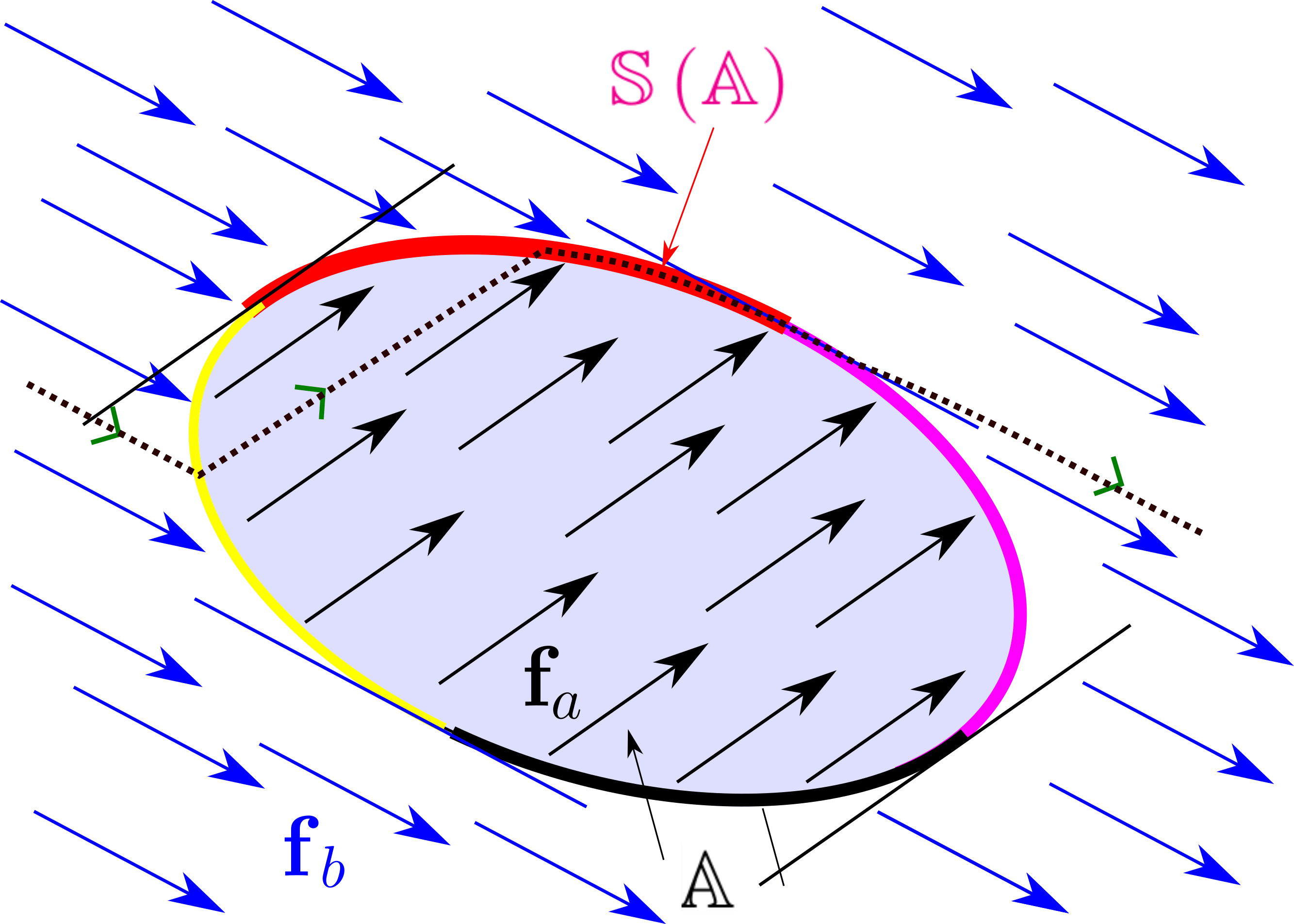
Figure 2: Sliding surface $\mathbb{S}\left(\mathbb{A}\right)$ (red) for $\mathbb{A}=\left\{\mathbf{x}|c\left(\mathbf{x}\right)\leq 0\right\}$

We recall the following result that has been proved in [17].

Proposition 2.1.

Consider two closed sets $\mathbb{A}_{1}$ and $\mathbb{A}_{2}$. As illustrated by Figure 3, we have

$$\begin{array}[]{cccc}(i)&\mathbb{S}\left(\mathbb{A}_{1}\cap\mathbb{A}_{2}\right)&=&\left(\mathbb{S}\left(\mathbb{A}_{1}\right)\cap\mathbb{A}_{2}\right)\cup\left(\mathbb{S}\left(\mathbb{A}_{2}\right)\cap\mathbb{A}_{1}\right)\\ (ii)&\mathbb{S}\left(\mathbb{A}_{1}\cup\mathbb{A}_{2}\right)&=&\left(\mathbb{S}\left(\mathbb{A}_{1}\right)\cap\overline{\mathbb{A}_{2}}\right)\cup\left(\mathbb{S}\left(\mathbb{A}_{2}\right)\cap\overline{\mathbb{A}_{1}}\right)\end{array}$$ (6)

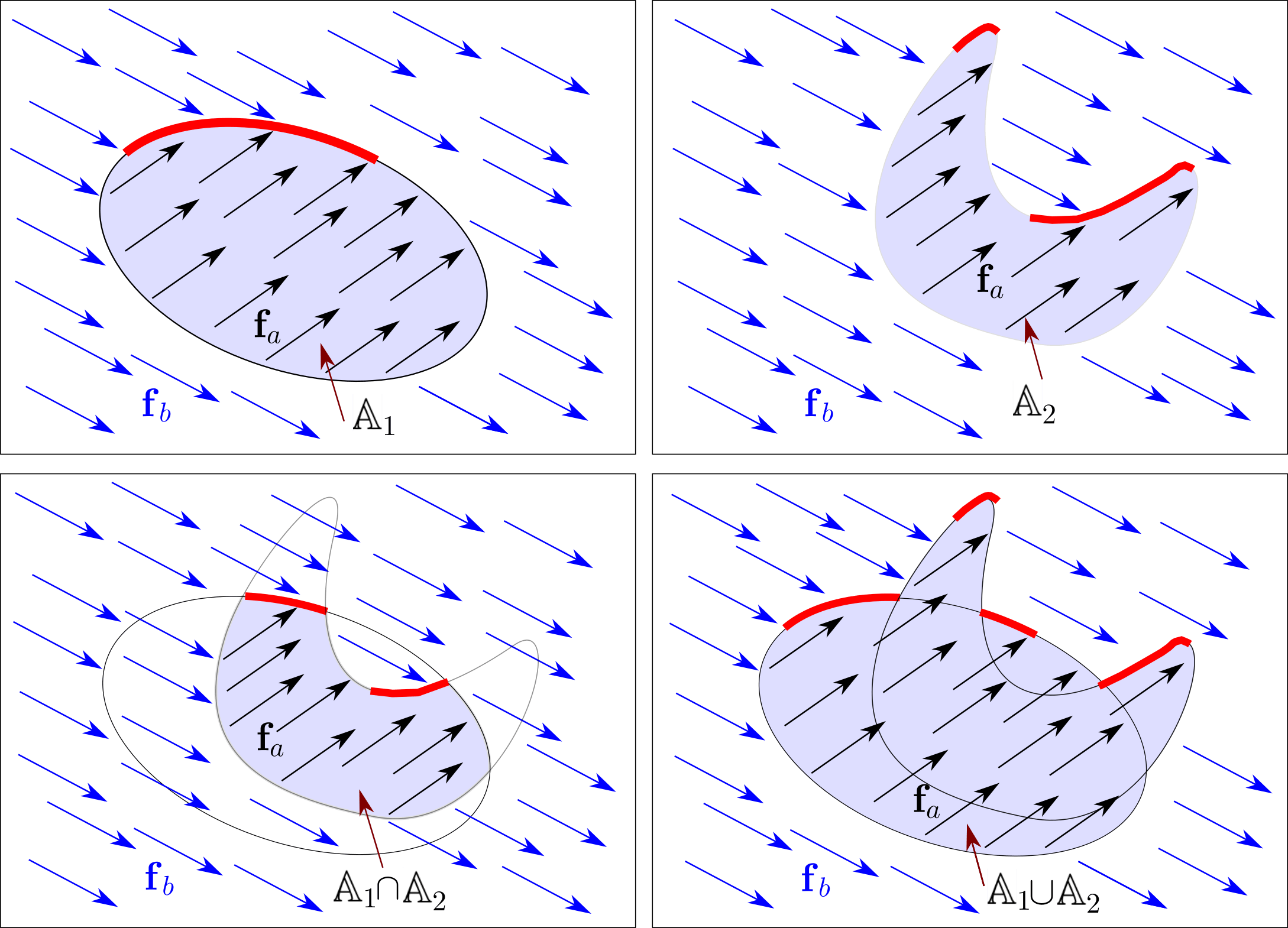
Figure 3: Illustration of Proposition 2.1, the sliding surfaces are painted red

Proposition 2.1 can be used to compute the sliding surface of a set $\mathbb{A}$ as soon as $\mathbb{A}$ can be defined by inequalities connected by Boolean operators such as and, or, not. The proposition is illustrated by Figure 4 in the case where $\mathbb{A}=\mathbb{A}_{1}\cup\left(\mathbb{A}_{2}\cap\mathbb{A}_{3}\right)$ and $\mathbb{A}_{i}=\left\{\mathbf{x}|c_{i}\left(\mathbf{x}\right)\leq 0\right\}$. The trajectory (green) slides twice, first on $\partial\mathbb{A}_{1}$, then it slides on $\partial\mathbb{A}_{2}$. The sliding surfaces are painted red.

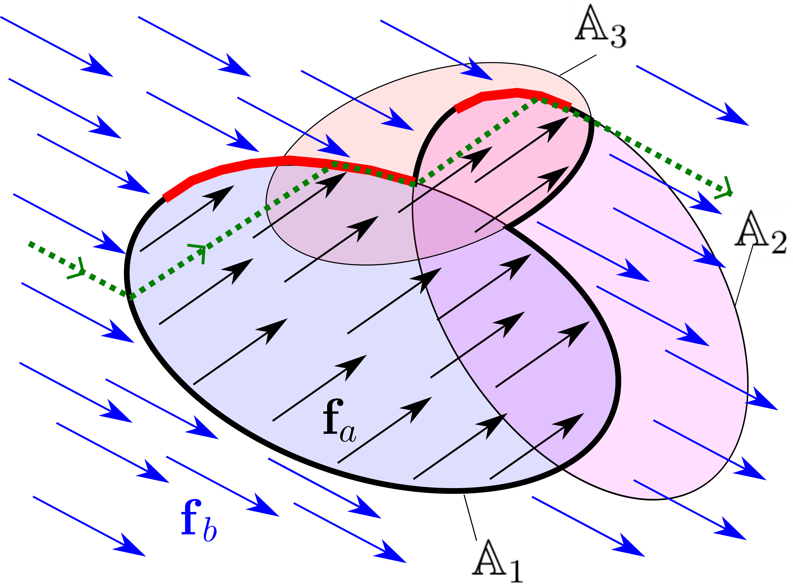
Figure 4: Sliding surfaces for $\mathbb{A}=\mathbb{A}_{1}\cup\left(\mathbb{A}_{2}\cap\mathbb{A}_{3}\right)$

2.5 Sliding surface in case of uncertainties

In case of uncertainties, the system defined in (1) can be described as

$$\begin{array}[]{c}\mathcal{S}_{\mathbf{p}}:\begin{array}[]{c}\left\{\begin{array}[]{ccc}\dot{\mathbf{x}}=\mathbf{f}_{a}\left(\mathbf{x}\right)&&\text{if $\mathbf{x}\in\mathbb{A}$}\\ \dot{\mathbf{x}}=\mathbf{f}_{b}\left(\mathbf{x}\right)&&\text{if $\mathbf{x}\in\overline{\mathbb{A}}$}\end{array}\right.\end{array}\end{array}$$

but now, $\mathbb{A},\mathbf{f}_{a},\mathbf{f}_{b}$ are uncertain. For instance, they may depend on a parameter vector $\mathbf{p}\in[\mathbf{p}]$ which models the uncertainties. Recall that from Equation 5, the sliding surface satisfies

$$\begin{array}[]{ccl}\mathbb{S}&=&\partial\mathbb{A}\cap\overline{\mathbb{L}_{a}^{c}}\,\cap\mathbb{L}_{b}^{c}\end{array}$$

Assume that

$$\left\{\begin{array}[]{c}\mathbb{A}^{\subset}\subset\mathbb{A}\subset\mathbb{A}^{\supset}\\ \mathbb{L}_{a}^{c\,\subset}\subset\mathbb{L}_{a}^{c}\subset\mathbb{L}_{a}^{c\,\supset}\\ \mathbb{L}_{b}^{c\,\subset}\subset\mathbb{L}_{b}^{c}\subset\mathbb{L}_{b}^{c\,\supset}\end{array}\right.$$

The sliding surface satisfies

$$\underset{\mathbb{S}^{\subset}}{\underbrace{\partial\mathbb{A}^{\subset}\cap\overline{\mathbb{L}_{a}^{c\supset}}\,\cap\mathbb{L}_{b}^{c\subset}}}\subset\mathbb{S}\subset\underset{\mathbb{S}^{\supset}}{\underbrace{\partial\mathbb{A}^{\supset}\cap\overline{\mathbb{L}_{a}^{c\subset}}\,\cap\mathbb{L}_{b}^{c\supset}}}$$

and we can write

$$\mathbb{S}\in[\negthinspace[\mathbb{S^{\subset}},\mathbb{S}^{\supset}]\negthinspace]=\partial[\negthinspace[\mathbb{A^{\subset}},\mathbb{A}^{\supset}]\negthinspace]\cap\overline{[\negthinspace[\mathbb{L}_{a}^{c\,\subset},\mathbb{L}_{a}^{c\,\supset}]\negthinspace]}\,\cap[\negthinspace[\mathbb{L}_{b}^{c\,\subset},\mathbb{L}_{b}^{c\,\supset}]\negthinspace]$$

using the thick set formalism described in the following section. In our application, is is clear that $\mathbb{S}^{\subset}=\emptyset$, since the set to be enclosed is a surface that has no volume. The set $\mathbb{S}^{\supset}$ is an upper approximation of this surface as illustrated by Figure 5.

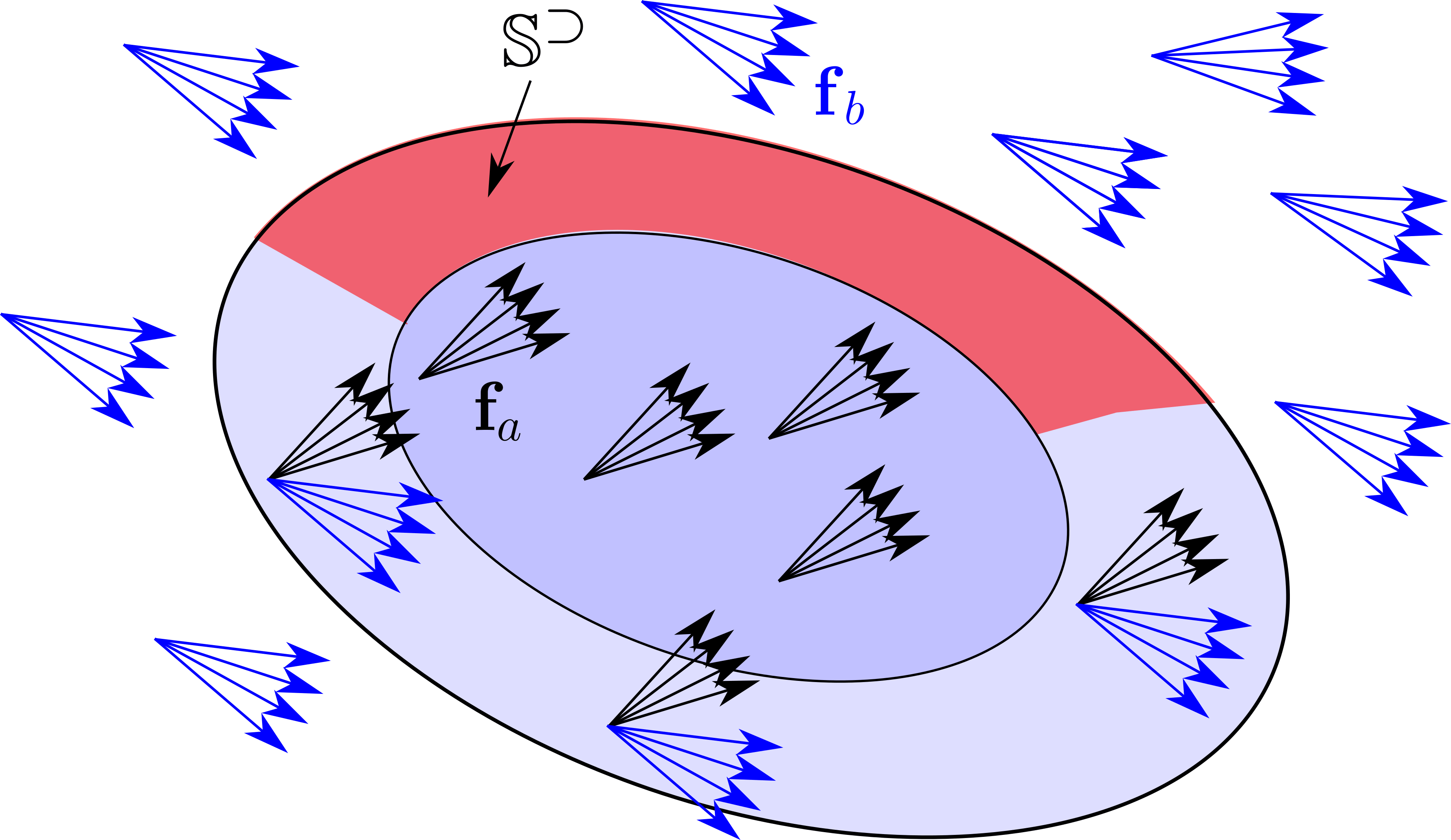
Figure 5: The set $\mathbb{S}^{\supset}$ (red) is an upper approximation of the sliding surface $\mathbb{S}_{\mathbf{p}}$ to be enclosed

3 Thick sets

When dealing with uncertainties, the evolution equation involved in Equation 1 and the sets $\mathbb{A},\mathbb{B}$ become uncertain. The sliding surface to be computed becomes thick and now has an interior. To compute an inner and an outer approximation of this approximation, we now introduce the recent concept of thick set with the associated algebra [11].

3.1 Definition

If an interval of $\mathbb{R}$ is an uncertain real number, a thick set is an uncertain subset of $\mathbb{R^{\textnormal{$n$}}}$. More precisely, a thick set is an interval of the powerset of $\mathbb{R}^{n}$ equipped with the inclusion $\subset$ as an order relation.

A thin set is a subset of $\mathbb{R^{\textnormal{$n$}}}$. It is qualified as thin because its boundary is thin.

Denote by $(\mathcal{P}(\mathbb{R}^{n}),\subset)$, the powerset of $\mathbb{R}^{n}$ equipped with the inclusion $\subset$ as an order relation. A thick set $[\negthinspace[\mathbb{X}]\negthinspace]$ of $\mathbb{R}^{n}$ is an interval of $(\mathcal{P}(\mathbb{R}^{n}),\subset)$. If $[\negthinspace[\mathbb{X}]\negthinspace]$ is a thick set of $\mathbb{R}^{n}$ , there exist two subsets of $\mathbb{R}^{n}$ , called the subset bound and the superset bound such that

$$[\negthinspace[\mathbb{X}]\negthinspace]=[\negthinspace[\mathbb{\mathbb{X}^{\subset}},\mathbb{X}^{\supset}]\negthinspace]=\{\mathbb{X}\in\mathcal{P}(\mathbb{R}^{n})|\mathbb{\mathbb{X}^{\subset}\subset\mathbb{X}\subset\mathbb{X}^{\supset}}\}.$$ (7)

The subset $\mathbb{X}^{\supset}\backslash\mathbb{X}^{\subset}$ is called the penumbra and plays an important role in the characterization of thick sets [10]. Thick sets can be used to represent uncertain sets (such as an uncertain map [12]) or soft constraints [7]. It can also can also be extended to fuzzy sets as shown in [14][6].

3.2 Algebra

We now show how we can define operations for thick sets (as a union, intersection, difference, etc.). The main motivation is to be able to compute with thick sets.

Consider two thick sets $[\negthinspace[\mathbb{X}]\negthinspace]=[\negthinspace[\mathbb{\mathbb{X}^{\subset}},\mathbb{X}^{\supset}]\negthinspace]$ and $[\negthinspace[\mathbb{Y}]\negthinspace]=[\negthinspace[\mathbb{\mathbb{Y}^{\subset}},\mathbb{Y}^{\supset}]\negthinspace]$. We define the following operations [10] which corresponds to an interval extension in the sense of Moore [23] applied to thick sets:

$$\begin{array}[]{ccc}[\negthinspace[\mathbb{X}]\negthinspace]\cap[\negthinspace[\mathbb{Y}]\negthinspace]&=&[\negthinspace[\mathbb{\mathbb{X}^{\subset}}\cap\mathbb{Y}^{\subset},\mathbb{X}^{\supset}\cap\mathbb{Y}^{\supset}]\negthinspace]\\ {}[\negthinspace[\mathbb{X}]\negthinspace]\cup[\negthinspace[\mathbb{Y}]\negthinspace]&=&[\negthinspace[\mathbb{\mathbb{X}^{\subset}}\cup\mathbb{Y}^{\subset},\mathbb{X}^{\supset}\cup\mathbb{Y}^{\supset}]\negthinspace]\\ \overline{[\negthinspace[\mathbb{X}]\negthinspace]}&=&[\negthinspace[\overline{\mathbb{X}^{\supset}},\overline{\mathbb{X}^{\subset}}]\negthinspace]\\ \partial[\negthinspace[\mathbb{X}]\negthinspace]&=&[\negthinspace[\mathbb{X}]\negthinspace]\cap\overline{[\negthinspace[\mathbb{X}]\negthinspace]}\\ \mathbf{f}([\negthinspace[\mathbb{X}]\negthinspace])&=&[\negthinspace[\mathbf{f}(\mathbb{\mathbb{X}^{\subset}}),\mathbf{f}(\mathbb{X}^{\supset})]\negthinspace]\\ \mathbf{f}^{-1}([\negthinspace[\mathbb{X}]\negthinspace])&=&[\negthinspace[\mathbf{f}^{-1}(\mathbb{\mathbb{X}^{\subset}}),\mathbf{f}^{-1}(\mathbb{X}^{\supset})]\negthinspace]\end{array}$$ (8)

We could also have defined these operations as follows:

$$\,\begin{array}[]{ccc}[\negthinspace[\mathbb{X}]\negthinspace]\diamond[\negthinspace[\mathbb{Y}]\negthinspace]&=&[\negthinspace[\bigcap\left\{\mathbb{X}\diamond\mathbb{Y},\mathbb{X}\in[\negthinspace[\mathbb{X}]\negthinspace],\mathbb{Y}\in[\negthinspace[\mathbb{Y}]\negthinspace]\right\},\bigcup\left\{\mathbb{X}\diamond\mathbb{Y},\mathbb{X}\in[\negthinspace[\mathbb{X}]\negthinspace],\mathbb{Y}\in[\negthinspace[\mathbb{Y}]\negthinspace]\right\}]\negthinspace]\end{array}$$

where $\diamond$ is a binary operator on sets such as $\cup,\cap,\backslash,\dots$, and

$$\phi[\negthinspace[\mathbb{X}]\negthinspace]=[\negthinspace[\bigcap\left\{\phi(\mathbb{X}),\mathbb{X}\in[\negthinspace[\mathbb{X}]\negthinspace]\right\},\bigcup\left\{\phi(\mathbb{X}),\mathbb{X}\in[\negthinspace[\mathbb{X}]\negthinspace]\right\}]\negthinspace]$$

where $\phi$ is a unary operator on sets such as $\partial\mathbb{X},\overline{\mathbb{X}},\dots$

Some of these operations are illustrated by Figure 6. The first subfigure represents the thick set $[\negthinspace[\mathbb{X}]\negthinspace]=[\negthinspace[\mathbb{\mathbb{X}^{\subset}},\mathbb{X}^{\supset}]\negthinspace]$. The lower bound $\mathbb{\mathbb{X}^{\subset}}$ is painted red; the penumbra $\mathbb{X}^{\supset}\backslash\mathbb{X}^{\subset}$ is painted orange; and all $\mathbf{x}$ outside the upper bound $\mathbb{X}^{\supset}$ of $[\negthinspace[\mathbb{X}]\negthinspace]$ is in blue.

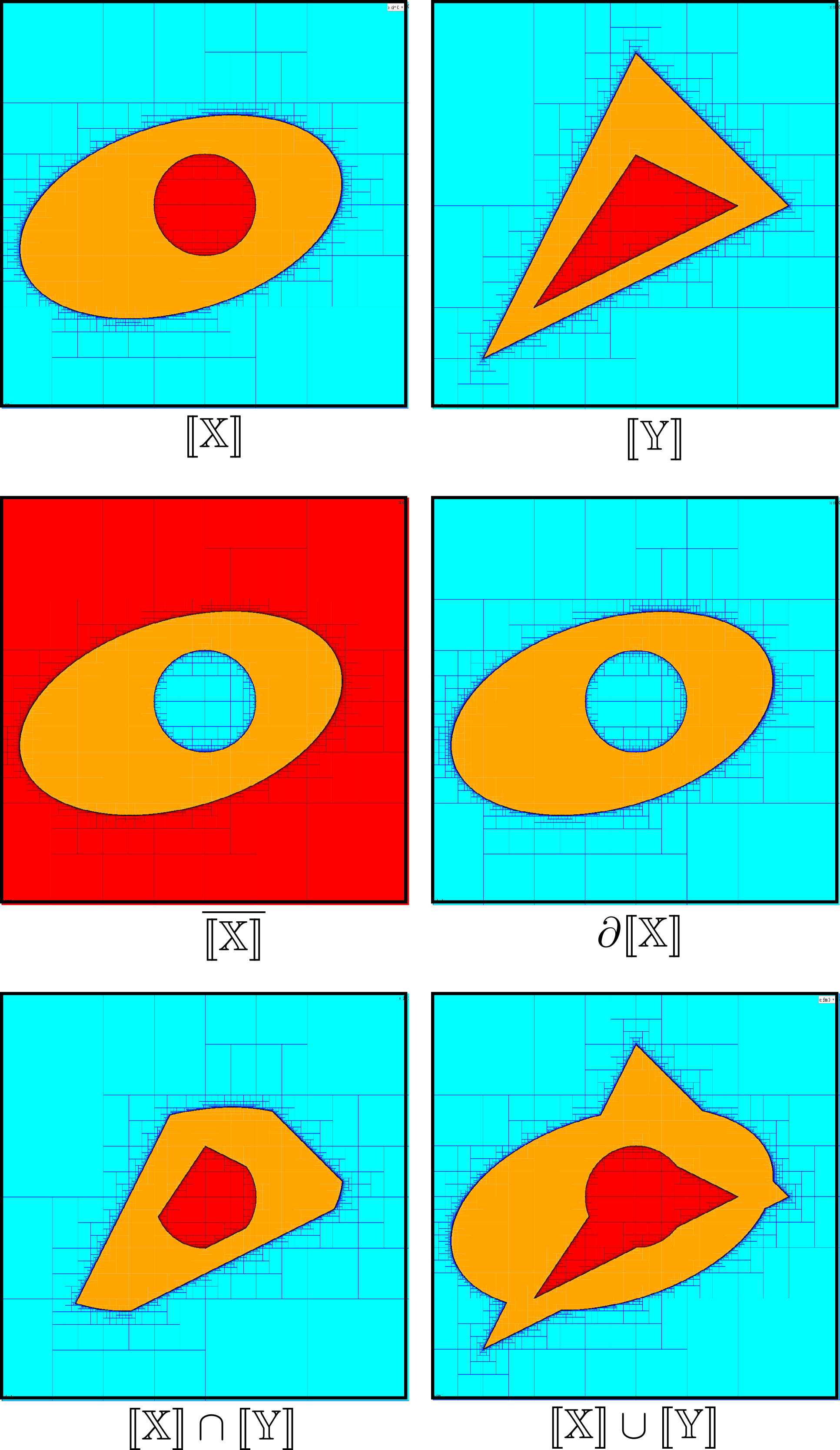
Figure 6: Operations between two thick sets. Red means inside, Blue means outside and Orange is for the penumbra

3.3 Atoms

To compute with thick sets, we first need to generate elementary thick sets, called the atoms. They can be given by geometrical sets such as boxes, polygons or disks. They can also constructed from an expression of the form $f(\mathbf{x},\mathbf{p})\leq 0$, where $f:\mathbb{R}^{n}\times\mathbb{R}^{m}\rightarrow\mathbb{R}$ and $\mathbf{p}\in[\mathbf{p}]$ is the parameter vector. This can be done by the following operator

$$[\negthinspace[\sigma]\negthinspace](f,[\mathbf{p}])=[\negthinspace[\mathbb{\mathbb{X}^{\subset}},\mathbb{X}^{\supset}]\negthinspace]$$

with

$$\begin{array}[]{ccc}\mathbb{\mathbb{X}^{\subset}}&=&\{\mathbf{x}|\forall\mathbf{p}\in[\mathbf{p}]f(\mathbf{x},\mathbf{p})\leq 0\}\\ \mathbb{X}^{\supset}&=&\{\mathbf{x}|\exists\mathbf{p}\in[\mathbf{p}]f(\mathbf{x},\mathbf{p})\leq 0\}.\end{array}$$

4 Characterizing the sliding surface of an uncertain controlled child swing

In this section, we propose an original academical example which illustrates how the thick set algebra can be used to characterize sliding surfaces of uncertain hybrid systems.

4.1 Pendulum

Consider a pendulum depicted in Figure 7, left. Its state representation is

$$\begin{array}[]{lll}\left(\begin{array}[]{c}\dot{x}_{1}\\ \dot{x}_{2}\end{array}\right)&=&\left(\begin{array}[]{c}x_{2}\\ -\sin x_{1}+p_{1}+u\end{array}\right)\end{array}$$

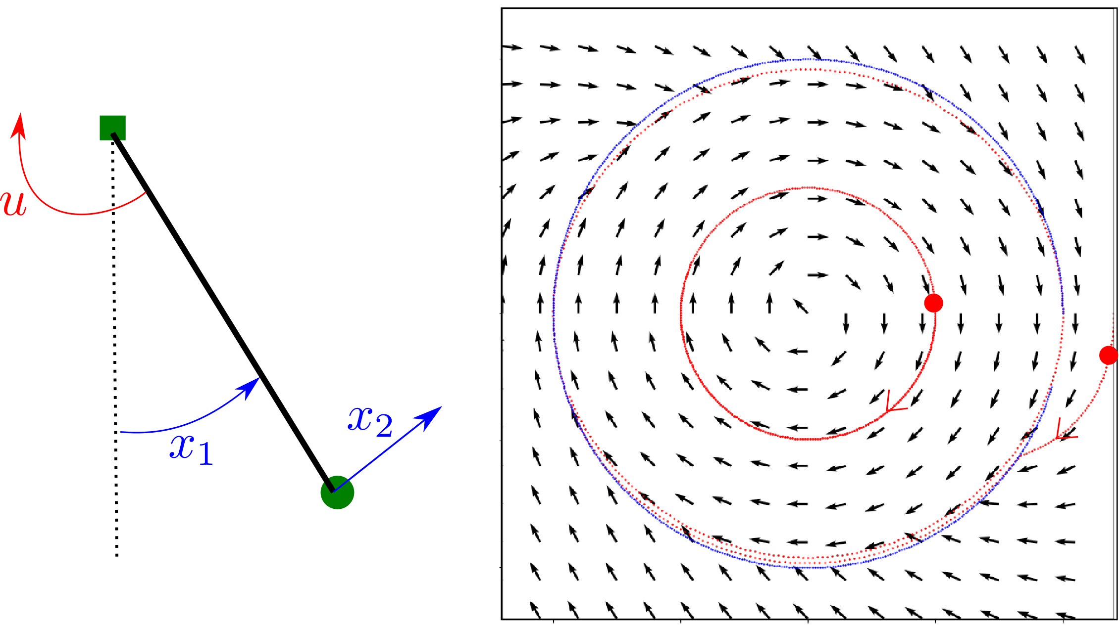
Figure 7: Child swing with state vector $\mathbf{x}=\left(x_{1},x_{2}\right)$

The pendulum represents a child swing, $u$ is a security break and $p_{1}$ is a perturbation which can be associated to the force generated by the child. In a nominal behavior, we have, $u=0$ but when the energy of the swing becomes too large, the controller generates a friction $u=-x_{2}$ to slow down the swing. More precisely, the following controller is:

$$\text{ if }c(\mathbf{x})<0\text{ then }u=0\text{ else $u=-x_{2}$,}$$

where $c(\mathbf{x})=x_{1}^{2}+x_{2}^{2}-1$ plays the role of the energy. The corresponding vector field is represented in Figure 7, right with two different trajectories (red) for $p_{1}=0$.

4.2 Thick approximation of the sliding surface

Assume that, when the controller alternates indefinitely between $u=0$ (break off) and $u=-x_{2}$ (break on), the controller may be damaged. We want to compute the sliding states which can be difficult to detect with simulations.

We have the two fields

$$\mathbf{f}_{a}=\left(\begin{array}[]{c}x_{2}\\ p_{1}-\sin x_{1}\end{array}\right),\mathbf{f}_{b}=\left(\begin{array}[]{c}x_{2}\\ p_{1}-\sin x_{1}-x_{2}\end{array}\right)$$

where $p_{1}\in[p_{1}]$ is an uncertain variable. We have

$$\begin{array}[]{ccl}\mathcal{L}_{a}^{c}\left(\mathbf{x}\right)&=&\frac{dc}{d\mathbf{x}}\left(\mathbf{x}\right)\cdot\mathbf{f}_{a}\left(\mathbf{x}\right)\\ &=&\left(\begin{array}[]{cc}2x_{1}&2x_{2}\end{array}\right)\cdot\left(\begin{array}[]{c}x_{2}\\ p_{1}-\sin x_{1}\end{array}\right)\\ &=&2x_{1}x_{2}+2x_{2}(p_{1}-\sin x_{1})\end{array}$$ (9)

and

$$\begin{array}[]{cll}\mathcal{L}_{b}^{c}\left(\mathbf{x}\right)&=&\frac{dc}{d\mathbf{x}}\left(\mathbf{x}\right)\cdot\mathbf{f}_{b}\left(\mathbf{x}\right)\\ &=&\left(\begin{array}[]{cc}2x_{1}&2x_{2}\end{array}\right)\cdot\left(\begin{array}[]{c}x_{2}\\ p_{1}-\sin x_{1}-x_{2}\end{array}\right)\\ &=&2x_{1}x_{2}+2x_{2}(p_{1}-\sin x_{1}-x_{2})\end{array}$$

To take into account the fact that $x_{1}$ and $x_{2}$ are given to the controller with a given bounded error $p_{2}\in[p_{2}],p_{3}\in[p_{3}]$, we take

$$\mathbb{A}=\left\{\mathbf{x}|\left(x_{1}+p_{2}\right)^{2}+\left(x_{2}+p_{3}\right)^{2}-1\leq 0\right\}.$$

To compute the paving associated to the expression (5), we need to build the atoms $[\negthinspace[\mathbb{A}]\negthinspace],[\negthinspace[\mathbb{L}_{a}^{c}]\negthinspace],[\negthinspace[\mathbb{L}_{b}^{c}]\negthinspace]$ as explained in Subsection 3.3.

If we choose $[p_{i}]=[-0.1,0.1],\forall i$, we get the approximation represented by Figure 8, Left. It is obtained by the following statements

$$\begin{array}[]{ccl}1&&[p_{1}]:=[p_{2}]:=[p_{3}]:=[-0.1,0.1]\\ 2&&[\negthinspace[\mathbb{L}_{a}^{c}]\negthinspace]:=[\negthinspace[\sigma]\negthinspace](2x_{1}x_{2}+2x_{2}(p_{1}-\sin x_{1}),[p_{1}])\\ 3&&[\negthinspace[\mathbb{L}_{b}^{c}]\negthinspace]:=[\negthinspace[\sigma]\negthinspace](2x_{1}x_{2}+2x_{2}(p_{1}-\sin x_{1}-x_{2}),[p_{1}])\\ 4&&[\negthinspace[\mathbb{A}]\negthinspace]:=[\negthinspace[\sigma]\negthinspace](\left(x_{1}+p_{2}\right)^{2}+\left(x_{2}+p_{3}\right)^{2}-1,[p_{2}]\times[p_{3}])\\ 5&&[\negthinspace[\mathbb{S}]\negthinspace]:=\partial[\negthinspace[\mathbb{A}]\negthinspace]\cap\overline{[\negthinspace[\mathbb{L}_{a}^{c}]\negthinspace]}\,\cap[\negthinspace[\mathbb{L}_{b}^{c}]\negthinspace]\end{array}$$

We note that $\mathbb{S}^{\subset}=\emptyset$, which is consistent with the fact that the surface to be approximated has no volume. This is the reason why the outer approximation $\mathbb{S}^{\supset}$ of the surface $\mathbb{S}$ corresponds to the penumbra of the thick set $[\negthinspace[\mathbb{S}]\negthinspace]$.

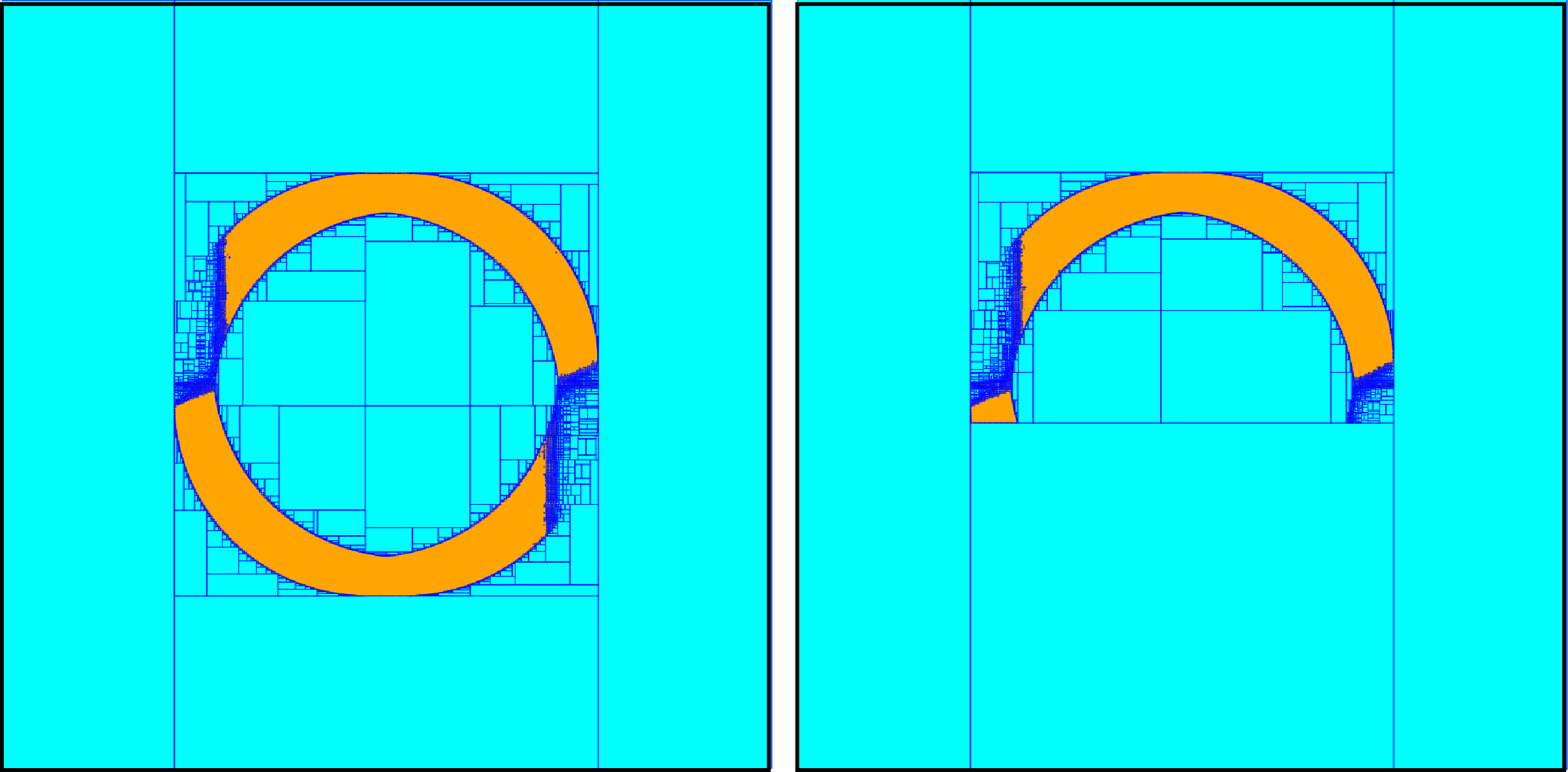
Figure 8: The orange zone corresponds to the outer approximation $\mathbb{S}^{\supset}$ of the sliding surface $\mathbb{S}$

4.2.1 One more condition

We extend our example by adding another condition in order to illustrate the facility of using thick set algebra to compute with uncertain sets.

To avoid to frighten the child on the swing, we want that when the swing goes strongly backward, the break does not switch on. More precisely, the controller becomes

$$\text{ if }\underset{c_{1}(\mathbf{x})}{\underbrace{x_{1}^{2}+x_{2}^{2}-1\leq 0}}\leq 0\text{ or $\underset{c_{2}(\mathbf{x})}{\underbrace{x_{2}+0.2}}$$\leq 0$ then }u=0\text{ else $u=-x_{2}$.}$$

The or condition can be treated using Proposition 2.1. We have

$$\begin{array}[]{ccc}\mathcal{L}_{a}^{c_{2}}\left(\mathbf{x}\right)&=&\frac{dc_{2}}{d\mathbf{x}}\left(\mathbf{x}\right)\cdot\mathbf{f}_{a}\left(\mathbf{x}\right)=p_{1}-\sin x_{1}\end{array}$$ (10)

and

$$\begin{array}[]{ccc}\mathcal{L}_{b}^{c_{2}}\left(\mathbf{x}\right)&=&\frac{dc_{2}}{d\mathbf{x}}\left(\mathbf{x}\right)\cdot\mathbf{f}_{b}\left(\mathbf{x}\right)=p_{1}-\sin x_{1}-x_{2}\end{array}$$ (11)

An enclosure $[\negthinspace[\mathbb{S}]\negthinspace]$ for the sliding surface $\mathbb{S}$ is represented by Figure 8, Right. It is obtained by the following statements

$$\begin{array}[]{ccl}1&&[p_{1}]:=[p_{2}]:=[p_{3}]:=[-0.1,0.1]\\ 2&&[\negthinspace[\mathbb{L}_{a}^{c_{1}}]\negthinspace]:=[\negthinspace[\sigma]\negthinspace](2x_{1}x_{2}+2x_{2}(p_{1}-\sin x_{1}),[p_{1}])\\ 3&&[\negthinspace[\mathbb{L}_{b}^{c_{1}}]\negthinspace]:=[\negthinspace[\sigma]\negthinspace](2x_{1}x_{2}+2x_{2}(p_{1}-\sin x_{1}-x_{2}),[p_{1}])\\ 4&&[\negthinspace[\mathbb{L}_{a}^{c_{2}}]\negthinspace]:=[\negthinspace[\sigma]\negthinspace](p_{1}-\sin x_{1},[p_{1}])\\ 5&&[\negthinspace[\mathbb{L}_{b}^{c_{2}}]\negthinspace]:=[\negthinspace[\sigma]\negthinspace](p_{1}-\sin x_{1}-x_{2},[p_{1}])\\ 6&&[\negthinspace[\mathbb{A}_{1}]\negthinspace]:=[\negthinspace[\sigma]\negthinspace](\left(x_{1}+p_{2}\right)^{2}+\left(x_{2}+p_{3}\right)^{2}-1,[p_{2}]\times[p_{3}])\\ 7&&[\negthinspace[\mathbb{A}_{2}]\negthinspace]:=[\negthinspace[\sigma]\negthinspace](x_{2}+0.2+p_{3},[p_{3}])\\ 8&&[\negthinspace[\mathbb{S}_{1}]\negthinspace]:=\partial[\negthinspace[\mathbb{A}_{1}]\negthinspace]\cap\overline{[\negthinspace[\mathbb{L}_{a}^{c_{1}}]\negthinspace]}\,\cap[\negthinspace[\mathbb{L}_{b}^{c_{1}}]\negthinspace]\\ 9&&[\negthinspace[\mathbb{S}_{2}]\negthinspace]:=\partial[\negthinspace[\mathbb{A}_{2}]\negthinspace]\cap\overline{[\negthinspace[\mathbb{L}_{a}^{c_{2}}]\negthinspace]}\,\cap[\negthinspace[\mathbb{L}_{b}^{c_{2}}]\negthinspace]\\ 10&&[\negthinspace[\mathbb{S}]\negthinspace]:=\left([\negthinspace[\mathbb{S}_{1}]\negthinspace]\cap\overline{[\negthinspace[\mathbb{A}_{2}]\negthinspace]}\right)\cup\left([\negthinspace[\mathbb{S}_{2}]\negthinspace]\cap\overline{[\negthinspace[\mathbb{A}_{1}]\negthinspace]}\right)\end{array}$$

A Python program associated with this example can be tested here:

www.ensta-bretagne.fr/jaulin/swing.html

5 Conclusion

In this paper, we have presented a new approach based on thick sets to enclose the sliding surfaces of a cyber-physical system in case of interval uncertainties. If the state of the system is on this sliding approximation, it may hesitate indefinitely between two different strategies. As a result, the system may be trapped on the sliding surface and the system may be damaged. It is thus important to compute an approximation of the sliding surface.

An expression given with thick sets can also be written as a quantified constraint satisfaction problem [25]. The main advantage of using a thick set expressions is that it corresponds to an interval extension of the thin set expression we want to compute. Thick sets is thus an interval representation of the uncertainties attached to the set we want to compute. Thick set arithmetic can also be interpreted as an interval arithmetic used to compute with uncertain subsets of $\mathbb{R}^{n}$, where as the classical interval arithmetic is used to compute with uncertain real numbers.

References

• [1]
• [2] E. Asarin, T. Dang & A. Girard (2007): Hybridization methods for the analysis of non-linear systems. Acta Informatica 7(43), pp. 451–476, 10.1007/s00236-006-0035-7.
• [3] E. Asarin, T. Dang & O. Maler (2002): The d/dt tool for verification of hybrid systems. In: In International Conference on Computer Aided Verification, Springer, pp. 365–370.
• [4] F. Blanchini & S. Miani (2007): Set-Theoretic Methods in Control. Springer Science & Business Media, 10.1007/978-3-319-17933-9.
• [5] O. Bouissou, A. Chapoutot, A. Djaballah & M. Kieffer (2014): Computation of parametric barrier functions for dynamical systems using interval analysis. In: 2014 IEEE 53rd Annual Conference on Decision and Control (CDC), pp. 753–758, 10.1109/CDC.2014.7039472.
• [6] R. Boukezzoula, L. Jaulin, B. Desrochers & D. Coquin (2020): Thick Fuzzy Sets and Their Potential Use in Uncertain Fuzzy Computations and Modeling. IEEE Transactions on Fuzzy Systems, 10.1109/TFUZZ.2020.3018550.
• [7] Q. Brefort, L. Jaulin, M. Ceberio & V. Kreinovich (2014): If we take into account that constraints are soft,then processing constraints Becomes algorithmically solvable. In: Proceedings of the IEEE Series of Symposia on Computational Intelligence SSCI’2014, Orlando, Florida, December 9-12, 10.1109/CIES.2014.7011823.
• [8] P. Cousot & R. Cousot (1977): Abstract Interpretation: A Unified Lattice Model for Static Analysis of Programs by Construction or Approximation of Fixpoints. In: Conference Record of the Fourth ACM Symposium on Principles of Programming Languages, Los Angeles, California, pp. 238–252.
• [9] N. Delanoue, L. Jaulin & B. Cottenceau (2006): Attraction domain of a nonlinear system using interval analysis. In: Twelfth International Conference on Principles and Practice of Constraint Programming (IntCP 2006), France, Nantes, pp. 181–189.
• [10] B. Desrochers & L. Jaulin (2017): Computing a guaranteed approximation the zone explored by a robot. IEEE Transaction on Automatic Control 62(1), pp. 425–430, 10.1109/TAC.2016.2530719.
• [11] B. Desrochers & L. Jaulin (2017): Thick set inversion. Artifical Intelligence 249, pp. 1–18, 10.1016/j.artint.2017.04.004.
• [12] B. Desrochers, S. Lacroix & L. Jaulin (2015): Set-Membership Approach to the Kidnapped Robot Problem. In: IROS 2015, 10.1109/IROS.2015.7353897.
• [13] S. Drakunov & V. Utkin (1992): Sliding mode control in dynamic systems. International Journal of Control 55(4), pp. 1029–1037, 10.1016/0005-1098(76)90076-5.
• [14] D. Dubois, L. Jaulin & H. Prade (2020): Thick Sets, Multiple-Valued Mappings and Possibility Theory, pp. 101–109. Springer.
• [15] G. Frehse (2008): PHAVer: Algorithmic Verification of Hybrid Systems. International Journal on Software Tools for Technology Transfer 10(3), pp. 23–48, 10.1007/s10009-007-0062-x.
• [16] E. Goubault & S. Putot (2006): Static Analysis of Numerical Algorithms. In: In Proceedings of SAS 06, LNCS 4134, Springer-Verlag, pp. 18–34.
• [17] L. Jaulin & F. Le Bars (2020): Characterizing sliding surfaces of cyber-physical systems. Acta Cybernetica 24, pp. 431–448, 10.4467/20838476SI.11.001.0287.
• [18] M. Konecny, W. Taha, J. Duracz, A. Duracz & A. Ames (2013): Enclosing the behavior of a hybrid system up to and beyond a Zeno point. In: Cyber-Physical Systems, Networks, and Applications (CPSNA), 10.1109/CPSNA.2013.6614258.
• [19] V. Kreinovich, A.V. Lakeyev, J. Rohn & P.T. Kahl (1997): Computational Complexity and Feasibility of Data Processing and Interval Computations. Reliable Computing 4(4), pp. 405–409, 10.1007/978-1-4757-2793-7.
• [20] T. Le Mézo, L. Jaulin & B. Zerr (2017): An interval approach to compute invariant sets. IEEE Transaction on Automatic Control 62, pp. 4236–4243, 10.1109/TAC.2017.2685241.
• [21] I. Mitchell (2007): Comparing forward and backward reachability as tools for safety analysis. In A. Bemporad, A. Bicchi & G. Buttazzo, editors: Hybrid Systems: Computation and Control, Springer-Verlag, pp. 428–443, 10.1109/4.16303.
• [22] I. Mitchell, A. Bayen & C. Tomlin (2001): Validating a Hamilton-Jacobi Approximation to Hybrid System Reachable Sets. In M. Benedetto & A. Sangiovanni-Vincentelli, editors: Hybrid Systems: Computation and Control, Lecture Notes in Computer Science 2034, Springer Berlin Heidelberg, pp. 418–432, 10.1006/jcph.1999.6345.
• [23] R. E. Moore (1979): Methods and Applications of Interval Analysis. SIAM, Philadelphia, PA, 10.1137/1.9781611970906.
• [24] N. Ramdani & N. Nedialkov (2011): Computing Reachable Sets for Uncertain Nonlinear Hybrid Systems using Interval Constraint Propagation Techniques. Nonlinear Analysis: Hybrid Systems 5(2), pp. 149–162, 10.1016/j.nahs.2010.05.010.
• [25] S. Ratschan (2002): Approximate Quantified Constraint Solving by Cylindrical Box Decomposition. Reliable Computing 8(1), pp. 21–42, 10.1023/A:1014785518570.
• [26] S. Ratschan & Z. She (2010): Providing a Basin of Attraction to a Target Region of Polynomial Systems by Computation of Lyapunov-like Functions. SIAM J. Control and Optimization 48(7), pp. 4377–4394, 10.1137/090749955.
• [27] A. Rauh & E. Auer (2009): Interval Approaches to Reliable Control of Dynamical Systems. In: Computer-assisted proofs - tools, methods and applications.
• [28] S. Rohou, L. Jaulin, M. Mihaylova, F. Le Bars & S. Veres (2018): Reliable non-linear state estimation involving time uncertainties. Automatica, pp. 379–388, 10.1016/j.automatica.2018.03.074.
• [29] S. Romig, L. Jaulin & A. Rauh (2019): Using Interval Analysis to Compute the Invariant Set of a Nonlinear Closed-Loop Control System. Algorithms 12(262), 10.3390/a12120262.
• [30] P. Saint-Pierre (2002): Hybrid kernels and capture basins for impulse constrained systems. In C.J. Tomlin & M.R. Greenstreet, editors: in Hybrid Systems: Computation and Control, 2289, Springer-Verlag, pp. 378–392, 10.1007/3-540-48983-5.
• [31] J. Alexandre Dit Sandretto & A. Chapoutot (2016): Validated Simulation of Differential Algebraic Equations with Runge-Kutta Methods. Reliable Computing 22.
• [32] W. Taha & A. Duracz (2015): Acumen: An Open-source Testbed for Cyber-Physical Systems Research. In: CYCLONE’15, 10.1007/978-3-319-47063-4_11.
• [33] D. Wilczak & P. Zgliczynski (2011): Cr-Lohner algorithm. Schedae Informaticae 20, pp. 9–46, 10.4467/20838476SI.11.001.0287.