High-order FDTD schemes for Maxwell’s interface problems with discontinuous coefficients and complex interfaces based on the Correction Function Method

Abstract

We propose high-order FDTD schemes based on the Correction Function Method (CFM) [5] for Maxwell’s interface problems with discontinuous coefficients and complex interfaces. The key idea of the CFM is to model the correction function near an interface to retain the order of a finite difference approximation. For this, we solve a system of PDEs based on the original problem by minimizing an energy functional. The CFM is applied to the standard Yee scheme and a fourth-order FDTD scheme. The proposed CFM-FDTD schemes are verified in 2-D using the transverse magnetic mode (TM_z). Numerical examples include scattering of magnetic and non-magnetic dielectric cylinders, and problems with manufactured solutions using various complex interfaces and discontinuous piecewise varying coefficients. Long-time simulations are also performed to provide numerical evidences of the stability of the proposed numerical approach. The proposed CFM-FDTD schemes achieve up to fourth-order convergence in $L^{2}$-norm and provide approximations devoid of spurious oscillations.

1 Introduction

In computational electromagnetics, the development of finite difference (FD) strategies to tackle Maxwell’s interface problems remains a challenge [1]. Indeed, one should expect from a numerical approach to treat arbitrary complex geometries of the interface without increasing the complexity of the method, achieve high-order convergence to diminish the phase error for long-time simulations [2] and handle discontinuous coefficients and discontinuous solutions, to name a few. The potential lack of regularity of the solution of such problems is a well-known challenge [3, 4, 5]. Moreover, FD schemes often use simple Cartesian mesh grids and therefore the representation of the interface and the enforcement of interface conditions, fundamental to obtain accurate results, are far from trivial. Hence, a first approach that consists of a staircased approximation of the interface and the use of the well-known Yee scheme [6], which is a second-order finite-difference time-domain (FDTD) scheme, yields a first-order scheme at best and non-convergent approximations in some cases [7].

Several numerical strategies have been proposed to overcome these issues. A staircase-free second-order FDTD scheme is proposed in [7] which explicitly enforces interface conditions. This numerical strategy has been verified for non-magnetic dielectric and perfect electric conductor (PEC) problems using a 2-D transverse magnetic (TM) form of Maxwell’s equations [7, 8]. Inspired by the Immersed Interface Method (IIM) [3], an Upwinding Embedded Boundary (UEB) method has also been developed to obtain a global second-order scheme to treat magnetic and non-magnetic dielectric problems using a TM form of Maxwell’s equations [9]. In the same vein, high-order FDTD schemes based on the Matched Interface and Boundary (MIB) method have been proposed in [10]. These strategies derive and use jump conditions to correct a finite difference approximation in the vicinity of the interface. MIB-based strategies were originally limited to non-magnetic dielectrics [10, 11] but later generalized to consider a discontinuous electromagnetic field at the interface [1, 12] using 2-D forms of Maxwell’s equations. However, the use of complex interfaces and high-order partial derivatives in jump conditions increase the complexity of MIB strategies as its order increases [10, 13].

Another avenue consists of FDTD schemes based on the Correction Function Method (CFM) [5]. Assuming that jumps on the interface can be smoothly extended in its vicinity, the CFM models corrections that are needed to retain the order of a finite difference approximation close to the interface by a system of PDEs based on the original problem. The solution of this system of PDEs is referred as the correction function. Approximations of the correction function are then computed, where it is needed, by minimizing a functional which is a square measure of the error associated with the correction function’s system of PDEs. Hence, high-order FDTD schemes can be generated for complex interfaces without significantly increasing the complexity of the proposed numerical strategy. The computational cost increases when compared with the original (i.e.​ without correction) FD scheme. Additionally, a parallel implementation of the CFM can be easily performed since minimization problems needed for the CFM are independent [14]. High-order FD schemes based on the CFM have been originally developed for 2-D Poisson’s equation with piecewise constant coefficients [5, 15, 16] as well as 3-D Poisson problems with interface jump conditions [17]. In computational electromagnetics, the CFM has been extended to the wave equation [18] and Maxwell’s equations [17] with constant coefficients. It is also worth mentioning that high-order CFM-FDTD schemes have been proposed to handle embedded PEC problems [19].

The work presented here generalizes CFM-FDTD approaches to Maxwell’s interface problems with discontinuous coefficients. We consider two FDTD schemes, namely the Yee scheme and a fourth-order staggered FDTD scheme, and correct them following the procedure described in [19]. In addition to scattering of dielectric cylinder problems, we also use problems with a manufactured solution for which complete discontinuous electromagnetic fields are considered to demonstrate the robustness and accuracy of the proposed numerical strategy. Finally, we show that the correction function implicitly provides the appropriate high-order jump conditions. Consequently, high-order explicit jump conditions [10, 1] are not required for the presented method.

The paper is organized as follows. In Section 2, we introduce Maxwell’s interface problem. The Correction Function Method is described in Section 3. In this same section, we introduce the functional to be minimized based on Maxwell’s equations with interface conditions. Then, numerical examples are performed in Section 4 to verify properties of the proposed CFM-FDTD schemes. Finally, we provide conclusion and outlook in Section 5.

2 Definition of the Problem

Assume a domain in space $\Omega$ subdivided into two subdomains $\Omega^{+}$ and $\Omega^{-}$, and a time interval $I=[0,T]$. The interface $\Gamma$ between subdomains is independent of time and allows the solutions to be discontinuous. Figure 1 illustrates a typical geometry of a domain $\Omega$.

Figure 1: Geometry of a domain $\Omega$ with an interface $\Gamma$.

For a given variable $\mathbold{A}$, we define $\mathbold{A}^{+}$ and $\mathbold{A}^{-}$ as respectively the solutions in $\Omega^{+}$ and $\Omega^{-}$. A jump of $\mathbold{A}$ on the interface $\Gamma$ is denoted as $\llbracket\mathbold{A}\rrbracket=\mathbold{A}^{+}-\mathbold{A}^{-}$. Assuming linear media, we consider Maxwell’s equations with interface conditions that are given by

$$\mu(\mathbold{x})\,\partial_{t}\mathbold{H}+\nabla\times\mathbold{E}= \,\,0\quad\text{in }\Omega\times I,$$ (1a)

$$\epsilon(\mathbold{x})\,\partial_{t}\mathbold{E}-\nabla\times\mathbold{H}= \,\,0\quad\text{in }\Omega\times I,$$ (1b)

$$\nabla\cdot(\epsilon(\mathbold{x})\,\mathbold{E})= \,\,0\quad\text{in }\Omega\times I,$$ (1c)

$$\nabla\cdot(\mu(\mathbold{x})\,\mathbold{H})= \,\,0\quad\text{in }\Omega\times I,$$ (1d)

$$\hat{\mathbold{n}}\times\llbracket\mathbold{E}\rrbracket= \,\,0\quad\text{on }\Gamma\times I,$$ (1e)

$$\hat{\mathbold{n}}\times\llbracket\mathbold{H}\rrbracket= \,\,0\quad\text{on }\Gamma\times I,$$ (1f)

$$\hat{\mathbold{n}}\cdot\llbracket\epsilon(\mathbold{x})\,\mathbold{E}\rrbracket= \,\,0\quad\text{on }\Gamma\times I,$$ (1g)

$$\hat{\mathbold{n}}\cdot\llbracket\mu(\mathbold{x})\,\mathbold{H}\rrbracket= \,\,0\quad\text{on }\Gamma\times I,$$ (1h)

$$\mathbold{n}\times\mathbold{H}= \,\,\mathbold{g}_{1}(\mathbold{x},t)\quad\text{on }\partial\Omega\times I,$$ (1i)

$$\mathbold{n}\times\mathbold{E}= \,\,\mathbold{g}_{2}(\mathbold{x},t)\quad\text{on }\partial\Omega\times I,$$ (1j)

$$\mathbold{H}= \,\,\mathbold{H}(\mathbold{x},0)\quad\text{in }\Omega,$$ (1k)

$$\mathbold{E}= \,\,\mathbold{E}(\mathbold{x},0)\quad\text{in }\Omega,$$ (1l)

where $\mathbold{H}$ is the magnetic field, $\mathbold{E}$ is the electric field, $\mu(\mathbold{x})>0$ is the magnetic permeability, $\epsilon(\mathbold{x})>0$ is the electrical permittivity, $\mathbold{n}$ is the unit outward normal to $\partial\Omega$ and $\hat{\mathbold{n}}$ is the unit normal to the interface $\Gamma$ pointing toward $\Omega^{+}$. Interface conditions are given by equations (1e) to (1h) while boundary and initial conditions are given by equations (1i) to (1l). Physical parameters, that is $\mu$ and $\epsilon$, can be discontinuous on the interface. Without loss of generality, we assume that electromagnetic fields are at divergence-free in each subdomain.

3 Correction Function Method

The Correction Function Method (CFM) allows one to find a correction for a given FD approximation involving nodes that belong to different subdomains in order to retain its order. For this purpose, the CFM assumes that solutions in each subdomain can be extended across the interface $\Gamma$ in a small domain $\Omega_{\Gamma}\times I$, that is such that $\Omega_{\Gamma}\subset\Omega$ encloses $\Gamma$. A system of PDEs based on the original problem, namely Maxwell’s interface problem (1) in our case, models the extension of each variable around the interface. The solution of this system of PDEs is referred as the correction function. Afterward, we define a functional that is a square measure of the error associated with the correction function’s system of PDEs. Approximations of the correction function are then computed, where it is needed, using a minimization procedure. In practice, the interface is discretized and a local patch $\Omega_{\Gamma}^{h}\times I_{\Gamma}^{h}\subset\Omega_{\Gamma}\times I$ is defined for each node of its discretization. Moreover, the size of local patches depends on the considered FD scheme and should diminish as the mesh grid size diminishes (see Remark 3.1).

In the following, we derive the system of PDEs that models the smooth extension of each variable and therefore the correction function. The minimization problem based on the associated energy functional is also presented.

Let us first introduce some notations. The inner product in $L^{2}\big{(}\Omega_{\Gamma}^{h}\times I_{\Gamma}^{h}\big{)}$ is defined by

$$\langle\mathbold{v},\mathbold{w}\rangle=\int\limits_{I_{\Gamma}^{h}}\!\int\limits_{\Omega_{\Gamma}^{h}}\!\!\mathbold{v}\cdot\mathbold{w}\,\mathrm{d}V\,\mathrm{d}t$$

with $\|\mathbold{v}\|=\langle\mathbold{v},\mathbold{v}\rangle$, and we also use the notation

$$\langle\mathbold{v},\mathbold{w}\rangle_{\Gamma}=\int\limits_{I_{\Gamma}^{h}}\!\int\limits_{\Gamma\cap\Omega_{\Gamma}^{h}}\!\!\mathbold{v}\cdot\mathbold{w}\,\mathrm{d}S\,\mathrm{d}t$$

with $\|\mathbold{v}\|_{\Gamma}=\langle\mathbold{v},\mathbold{v}\rangle_{\Gamma}$ for legibility. Unlike previous CFM-FDTD schemes, we cannot explicitly model jumps $\mathbold{D}_{H}=\llbracket\mathbold{H}\rrbracket$ and $\mathbold{D}_{E}=\llbracket\mathbold{E}\rrbracket$ because of discontinuous coefficients. Hence, we first need to estimate $\mathbold{H}^{+}$, $\mathbold{E}^{+}$, $\mathbold{H}^{-}$ and $\mathbold{E}^{-}$ in the whole patch, and afterward compute an approximation of $\mathbold{D}_{H}$ and $\mathbold{D}_{E}$. The system of PDEs for correction functions is then given by

$$\mu^{+}(\mathbold{x})\,\partial_{t}\mathbold{H}^{+}+\nabla\times\mathbold{E}^{+}= \,\,0\quad\text{in }\Omega_{\Gamma}^{h}\times I_{\Gamma}^{h},$$ (2)

$$\epsilon^{+}(\mathbold{x})\,\partial_{t}\mathbold{E}^{+}-\nabla\times\mathbold{H}^{+}= \,\,0\quad\text{in }\Omega_{\Gamma}^{h}\times I_{\Gamma}^{h},$$

$$\nabla\cdot(\epsilon^{+}(\mathbold{x})\,\mathbold{E}^{+})= \,\,0\quad\text{in }\Omega_{\Gamma}^{h}\times I_{\Gamma}^{h},$$

$$\nabla\cdot(\mu^{+}(\mathbold{x})\,\mathbold{H}^{+})= \,\,0\quad\text{in }\Omega_{\Gamma}^{h}\times I_{\Gamma}^{h},$$

$$\mu^{-}(\mathbold{x})\,\partial_{t}\mathbold{H}^{-}+\nabla\times\mathbold{E}^{-}= \,\,0\quad\text{in }\Omega_{\Gamma}^{h}\times I_{\Gamma}^{h},$$

$$\epsilon^{-}(\mathbold{x})\,\partial_{t}\mathbold{E}^{-}-\nabla\times\mathbold{H}^{-}= \,\,0\quad\text{in }\Omega_{\Gamma}^{h}\times I_{\Gamma}^{h},$$

$$\nabla\cdot(\epsilon^{-}(\mathbold{x})\,\mathbold{E}^{-})= \,\,0\quad\text{in }\Omega_{\Gamma}^{h}\times I_{\Gamma}^{h},$$

$$\nabla\cdot(\mu^{-}(\mathbold{x})\,\mathbold{H}^{-})= \,\,0\quad\text{in }\Omega_{\Gamma}^{h}\times I_{\Gamma}^{h},$$

$$\hat{\mathbold{n}}\times\llbracket\mathbold{E}\rrbracket= \,\,0\quad\text{on }\Gamma\cap\Omega_{\Gamma}^{h}\times I_{\Gamma}^{h},$$

$$\hat{\mathbold{n}}\times\llbracket\mathbold{H}\rrbracket= \,\,0\quad\text{on }\Gamma\cap\Omega_{\Gamma}^{h}\times I_{\Gamma}^{h},$$

$$\hat{\mathbold{n}}\cdot\llbracket\epsilon(\mathbold{x})\,\mathbold{E}\rrbracket= \,\,0\quad\text{on }\Gamma\cap\Omega_{\Gamma}^{h}\times I_{\Gamma}^{h},$$

$$\hat{\mathbold{n}}\cdot\llbracket\mu(\mathbold{x})\,\mathbold{H}\rrbracket= \,\,0\quad\text{on }\Gamma\cap\Omega_{\Gamma}^{h}\times I_{\Gamma}^{h},$$

Following the procedure described in [20] to construct a functional that is a square measure of the error associated with system (2) leads to an ill-posed minimization problem. As in CFM-FDTD strategies for embedded perfect electric conductors [19], we can take advantage of FD approximations at previous time steps using fictitious interface conditions to retrieve a well-posed minimization problem. Fictitious interface conditions are given by

$$\hat{\mathbold{n}}_{1,i}^{\circ}\times(\mathbold{E}^{\circ}-\mathbold{E}^{\circ,*})= \,\,0\quad\text{on}\quad\Gamma_{1,i}^{\circ}\times I_{\Gamma}^{h}\quad\text{for}\quad i=1,\ldots,N_{1}^{\circ},$$ (3)

$$\hat{\mathbold{n}}_{2,i}^{\circ}\times(\mathbold{H}^{\circ}-\mathbold{H}^{\circ,*})= \,\,0\quad\text{on}\quad\Gamma_{2,i}^{\circ}\times I_{\Gamma}^{h}\quad\text{for}\quad i=1,\ldots,N_{2}^{\circ},$$

$$\hat{\mathbold{n}}_{3,i}^{\circ}\cdot(\mathbold{E}^{\circ}-\mathbold{E}^{\circ,*})= \,\,0\quad\text{on}\quad\Gamma_{3,i}^{\circ}\times I_{\Gamma}^{h}\quad\text{for}\quad i=1,\ldots,N_{3}^{\circ},$$

$$\hat{\mathbold{n}}_{4,i}^{\circ}\cdot(\mathbold{H}^{\circ}-\mathbold{H}^{\circ,*})= \,\,0\quad\text{on}\quad\Gamma_{4,i}^{\circ}\times I_{\Gamma}^{h}\quad\text{for}\quad i=1,\ldots,N_{4}^{\circ},$$

where $\circ$ is either $+$ or $-$ depending in which subdomain the fictitious interface $\Gamma_{k,i}^{\circ}$ belongs, $\hat{\mathbold{n}}_{k,i}^{\circ}$ is the normal associated with $\Gamma_{k,i}^{\circ}$, $N_{k}^{\circ}$ is the number of fictitious interfaces, and $\mathbold{H}^{\circ,*}$ and $\mathbold{E}^{\circ,*}$ are approximations of the magnetic field and the electric field that come from a FD scheme.

The quadratic functional to minimize is therefore given by

$$J(\mathbold{H}^{+}, \mathbold{E}^{+},\mathbold{H}^{-},\mathbold{E}^{-})=\frac{\ell_{h}}{2}\,\big{\|}\mu^{+}\,\partial_{t}\mathbold{H}^{+}+\nabla\times\mathbold{E}^{+}\big{\|}+\frac{\ell_{h}}{2}\,\big{\|}\epsilon^{+}\,\partial_{t}\mathbold{E}^{+}-\nabla\times\mathbold{H}^{+}\big{\|}$$

$$+ \,\,\frac{\ell_{h}}{2}\,\big{\|}\nabla\cdot(\epsilon^{+}\,\mathbold{E}^{+})\big{\|}+\frac{\ell_{h}}{2}\,\big{\|}\nabla\cdot(\mu^{+}\,\mathbold{H}^{+})\big{\|}+\frac{\ell_{h}}{2}\,\big{\|}\mu^{-}\,\partial_{t}\mathbold{H}^{-}+\nabla\times\mathbold{E}^{-}\big{\|}$$

$$+ \,\,\frac{\ell_{h}}{2}\,\big{\|}\epsilon^{-}\,\partial_{t}\mathbold{E}^{-}-\nabla\times\mathbold{H}^{-}\big{\|}+\frac{\ell_{h}}{2}\,\big{\|}\nabla\cdot(\epsilon^{-}\,\mathbold{E}^{-})\big{\|}+\frac{\ell_{h}}{2}\,\big{\|}\nabla\cdot(\mu^{-}\,\mathbold{H}^{-})\big{\|}$$

$$+ \,\,\frac{c_{p}}{2}\,\big{\|}\hat{\mathbold{n}}\times(\mathbold{E}^{+}-\mathbold{E}^{-})\big{\|}_{\Gamma}+\frac{c_{p}}{2}\,\big{\|}\hat{\mathbold{n}}\times(\mathbold{H}^{+}-\mathbold{H}^{-})\big{\|}_{\Gamma}$$

$$+ \,\,\frac{c_{p}}{2}\,\big{\|}\hat{\mathbold{n}}\cdot(\epsilon^{+}\,\mathbold{E}^{+}-\epsilon^{-}\,\mathbold{E}^{-})\big{\|}_{\Gamma}+\frac{c_{p}}{2}\,\big{\|}\hat{\mathbold{n}}\cdot(\mu^{+}\,\mathbold{H}^{+}-\mu^{-}\,\mathbold{H}^{-})\big{\|}_{\Gamma}$$

$$+ \,\,\frac{c_{f}}{2\,N_{E^{+}}}\,\sum_{i=1}^{N_{1}^{+}}\big{\|}\hat{\mathbold{n}}_{1,i}^{+}\times(\mathbold{E}^{+}-\mathbold{E}^{+,*})\big{\|}_{\Gamma_{1,i}^{+}}+\frac{c_{f}}{2\,N_{H^{+}}}\,\sum_{i=1}^{N_{2}^{+}}\big{\|}\hat{\mathbold{n}}_{2,i}^{+}\times(\mathbold{H}^{+}-\mathbold{H}^{+,*})\big{\|}_{\Gamma_{2,i}^{+}}$$

$$+ \,\,\frac{c_{f}}{2\,N_{E^{+}}}\,\sum_{i=1}^{N_{3}^{+}}\big{\|}\hat{\mathbold{n}}_{3,i}^{+}\cdot(\mathbold{E}^{+}-\mathbold{E}^{+,*})\big{\|}_{\Gamma_{3,i}^{+}}+\frac{c_{f}}{2\,N_{H^{+}}}\,\sum_{i=1}^{N_{4}^{+}}\big{\|}\hat{\mathbold{n}}_{4,i}^{+}\cdot(\mathbold{H}^{+}-\mathbold{H}^{+,*})\big{\|}_{\Gamma_{4,i}^{+}}$$

$$+ \,\,\frac{c_{f}}{2\,N_{E^{-}}}\,\sum_{i=1}^{N_{1}^{-}}\big{\|}\hat{\mathbold{n}}_{1,i}^{-}\times(\mathbold{E}^{-}-\mathbold{E}^{-,*})\big{\|}_{\Gamma_{1,i}^{-}}+\frac{c_{f}}{2\,N_{H^{-}}}\,\sum_{i=1}^{N_{2}^{-}}\big{\|}\hat{\mathbold{n}}_{2,i}^{-}\times(\mathbold{H}^{-}-\mathbold{H}^{-,*})\big{\|}_{\Gamma_{2,i}^{-}}$$

$$+ \,\,\frac{c_{f}}{2\,N_{E^{-}}}\,\sum_{i=1}^{N_{3}^{-}}\big{\|}\hat{\mathbold{n}}_{3,i}^{-}\cdot(\mathbold{E}^{-}-\mathbold{E}^{-,*})\big{\|}_{\Gamma_{3,i}^{-}}+\frac{c_{f}}{2\,N_{H^{-}}}\,\sum_{i=1}^{N_{4}^{-}}\big{\|}\hat{\mathbold{n}}_{4,i}^{-}\cdot(\mathbold{H}^{-}-\mathbold{H}^{-,*})\big{\|}_{\Gamma_{4,i}^{-}}$$

where $c_{p}>0$ and $c_{f}>0$ are penalization coefficient, $\ell_{h}$ is the characteristic length in space of the patch, $N_{E^{\circ}}=N_{1}^{\circ}+N_{3}^{\circ}$ and $N_{H^{\circ}}=N_{2}^{\circ}+N_{4}^{\circ}$. Integrals over the domain are scaled by $\ell_{h}$ to guarantee that all terms in the functional $J$ behave in a similar way when the computational grid is refined [20]. The problem statement is then

$$\text{Find }(\mathbold{H}^{+},\mathbold{E}^{+},\mathbold{H}^{-},\mathbold{E}^{-})\in V\times W\times V\times W\text{ such that }$$ (4)

$$\qquad(\mathbold{H}^{+},\mathbold{E}^{+},\mathbold{H}^{-},\mathbold{E}^{-})\in\underset{\begin{subarray}{c}\mathbold{v}^{+},\mathbold{v}^{-}\in V\\ \mathbold{w}^{+},\mathbold{w}^{-}\in W\end{subarray}}{\arg\min}J(\mathbold{v}^{+},\mathbold{w}^{+},\mathbold{v}^{-},\mathbold{w}^{-}),$$

where $W=V$. Let us recall that we assume divergence-free electromagnetic fields in each subdomain. We therefore minimize the functional $J$ in a space of divergence-free space-time polynomials, namely

$$V=\big{\{}\mathbold{v}\in\big{[}P^{k}\big{(}\Omega_{\Gamma}^{h}\times I^{h}_{\Gamma}\big{)}\big{]}^{3}:\nabla\cdot\mathbold{v}=0\big{\}},$$

where $P^{k}$ denotes the space of polynomials of degree $k$. It is worth mentioning that basis functions of $V$ are based on high-degree divergence-free basis functions proposed in [21].

Remark 3.1.

The size in space of local patches $\ell_{h}$ depends of the mesh grid size, that is $\ell_{h}=\beta\,\max\{\Delta x,\Delta y,\Delta z\}$, where $\beta$ is a positive constant. The choice of $\beta$ depends on the considered FD scheme and must allow the construction of enough fictitious interfaces within the local patch. To ease the implementation, local patches are taken aligned with the mesh grid and square in space. Fictitious interfaces are also aligned with the mesh grid to facilitate the computation of space-time interpolants that are needed in the minimization problem. We refer the reader to [19] for more details on the implementation of local patches and fictitious interface conditions.

Remark 3.2.

The initialization of CFM-FDTD schemes can be difficult because of time integrals involving $\mathbold{H}^{*}$ and $\mathbold{E}^{*}$. An initialization strategy has been developed for the Yee scheme and a fourth-order FDTD scheme based on a multistep method [19]. Another approach, which is specific to some applications, consists to assume that electromagnetic fields close to the interface remain unchanged for $t\leq t_{0}$.

Remark 3.3.

Using a truncation error analysis, one can show that the order of a CFM-FDTD scheme for Maxwell’s equations (1) is $\min\{n,k\}$ where $n$ is the order of the considered FD scheme and $k$ is the degree of space-time polynomial spaces used in minimization problem (4) [19].

Remark 3.4.

The correction function’s system of PDEs on which functional $J$ is based models the extension of each electromagnetic field in the vicinity of the interface while satisfying interface conditions. Hence, by construction and consistency, explicit jump conditions on the interface used for Matched Interface and Boundary based strategies [10, 1] should be implicitly satisfied. This claim is supported by numerical evidences presented in subsection 4.1.

Remark 3.5.

It is recalled that fictitious interface conditions are used to retrieve a well-posed minimization problem. Regarding the value of $c_{f}$, the priority should be given to interface conditions and therefore $c_{p}>c_{f}>0$. Moreover, $c_{f}$ should also diminish as the mesh grid size diminishes to enforce again interface conditions. As mentioned in [19], the stability analysis of a CFM-FDTD scheme that uses fictitious interface conditions (3) is not trivial. Despite the lack of a rigorous proof, $c_{f}=\alpha\,\Delta t$, where $\alpha$ is a positive constant sufficiently small, seems to avoid any stability issues. We also assume that the stability condition of a CFM-FDTD scheme should be close to the one associated with the original (i.e.​ without correction) FDTD scheme. This is corroborated with numerical results in [19] and the performed numerical examples in subsection 4.3.

4 Numerical Examples

In this section, we perform convergence analysis and long-time simulations in 2-D to verify the proposed numerical strategy. We consider the transverse magnetic (TM${}_{\text{z}}$) mode. Hence, for a domain $\Omega\subset\mathbb{R}^{2}$, Maxwell’s equations are simplified to

$$\mu(x,y)\,\partial_{t}H_{x}+\partial_{y}E_{z}= \,\,0\quad\text{in }\Omega\times I,$$ (5)

$$\mu(x,y)\,\partial_{t}H_{y}-\partial_{x}E_{z}= \,\,0\quad\text{in }\Omega\times I,$$

$$\epsilon(x,y)\,\partial_{t}E_{z}-\partial_{x}H_{y}+\partial_{y}H_{x}= \,\,0\quad\text{in }\Omega\times I,$$

$$\partial_{x}(\mu(x,y)\,H_{x})+\partial_{y}(\mu(x,y)\,H_{y})= \,\,0\quad\text{in }\Omega\times I,$$

with the associated interface, boundary and initial conditions. In this 2-D simplification of Maxwell’s equations, electromagnetic fields are continuous across the interface between the vacuum and a non-magnetic dielectric material. However, for a magnetic dielectric material, the electric field is still continuous across the interface while the magnetic field is discontinuous.

We consider two different FDTD schemes, namely the Yee scheme and a fourth-order FDTD scheme. The latter FDTD scheme also uses staggered grids in both space and time. More specifically, space derivatives are estimated with a fourth-order centered FD approximation for staggered grids while time derivatives are estimated using a fourth-order staggered free-parameter multistep method [22]. The associated CFM-FDTD schemes are then the CFM-Yee scheme and the CFM-4^th scheme. We refer to [19] for more details on the application of the CFM to these two FDTD schemes.

4.1 Scattering of a Dielectric Cylinder Problems

Let us consider a dielectric cylinder in free-space exposed to a TM_z excitation wave. The interface is a circle of radius $r_{0}=0.6$ centered at $(0,0)$. The exact solution in cylindrical coordinates is given by the real part of

$$H_{\theta}(r,\theta,t)= \,\,\left\{\begin{array}[]{l l}-\frac{\mathfrak{i}\,k^{-}}{\omega\,\mu^{-}}\displaystyle\sum_{n=-\infty}^{\infty}C_{n}^{\text{tot}}\,J_{n}^{\prime}(k^{-}\,r)\,e^{\mathfrak{i}\,(n\,\theta+\omega\,t)},&\text{if}\quad r\leq r_{0},\\ -\frac{\mathfrak{i}\,k^{+}}{\omega\,\mu^{+}}\displaystyle\sum_{n=-\infty}^{\infty}(\mathfrak{i}^{-n}\,J_{n}^{\prime}(k^{+}\,r)+C_{n}^{\text{scat}}\,H_{n}^{{(2)}^{\prime}}(k^{+}\,r))\,e^{\mathfrak{i}\,(n\,\theta+\omega\,t)},&\text{if}\quad r>r_{0},\end{array}\right.$$

$$H_{r}(r,\theta,t)= \,\,\left\{\begin{array}[]{l l}-\frac{1}{\omega\,\mu^{-}\,r}\displaystyle\sum_{n=-\infty}^{\infty}n\,C_{n}^{\text{tot}}\,J_{n}(k^{-}\,r)\,e^{\mathfrak{i}\,(n\,\theta+\omega\,t)},&\text{if}\quad r\leq r_{0},\\ -\frac{1}{\omega\,\mu^{+}\,r}\displaystyle\sum_{n=-\infty}^{\infty}n\,(\mathfrak{i}^{-n}\,J_{n}(k^{+}\,r)+C_{n}^{\text{scat}}\,H_{n}^{(2)}(k^{+}\,r))\,e^{\mathfrak{i}\,(n\,\theta+\omega\,t)},&\text{if}\quad r>r_{0},\end{array}\right.$$

$$E_{z}(r,\theta,t)= \,\,\left\{\begin{array}[]{l l}\displaystyle\sum_{n=-\infty}^{\infty}C_{n}^{\text{tot}}\,J_{n}(k^{-}\,r)\,e^{\mathfrak{i}\,(n\,\theta+\omega\,t)},&\text{if}\quad r\leq r_{0},\\ \displaystyle\sum_{n=-\infty}^{\infty}(\mathfrak{i}^{-n}\,J_{n}(k^{+}\,r)+C_{n}^{\text{scat}}\,H_{n}^{(2)}(k^{+}\,r))\,e^{\mathfrak{i}\,(n\,\theta+\omega\,t)},&\text{if}\quad r>r_{0},\end{array}\right.$$

with

$$C_{n}^{\text{tot}}= \,\,\mathfrak{i}^{-n}\,\frac{\tfrac{k^{+}}{\mu^{+}}\,(J_{n}^{\prime}(k^{+}\,r_{0})\,H_{n}^{(2)}(k^{+}\,r_{0})-H_{n}^{{(2)}^{\prime}}(k^{+}\,r_{0})\,J_{n}(k^{+}\,r_{0}))}{\frac{k^{-}}{\mu^{-}}\,J_{n}^{\prime}(k^{-}\,r_{0})\,H_{n}^{(2)}(k^{+}\,r_{0})-\tfrac{k^{+}}{\mu^{+}}\,H_{n}^{{(2)}^{\prime}}(k^{+}\,r_{0})\,J_{n}(k^{-}\,r_{0})},$$

$$C_{n}^{\text{scat}}= \,\,\mathfrak{i}^{-n}\,\frac{\tfrac{k^{+}}{\mu^{+}}\,J_{n}^{\prime}(k^{+}\,r_{0})\,J_{n}(k^{-}\,r_{0})-\tfrac{k^{-}}{\mu^{-}}\,J_{n}^{\prime}(k^{-}\,r_{0})\,J_{n}(k^{+}\,r_{0})}{\frac{k^{-}}{\mu^{-}}\,J_{n}^{\prime}(k^{-}\,r_{0})\,H_{n}^{(2)}(k^{+}\,r_{0})-\tfrac{k^{+}}{\mu^{+}}\,H_{n}^{{(2)}^{\prime}}(k^{+}\,r_{0})\,J_{n}(k^{-}\,r_{0})},$$

where $\mathfrak{i}$ is the imaginary number, $k^{\circ}=\omega\,\sqrt{\mu^{\circ}\,\epsilon^{\circ}}$, $\omega=2\,\pi$, $J_{n}$ is the $n$-order Bessel function of first kind and $H_{n}^{(2)}$ is the $n$-order Hankel function of second kind [23, 9].

For the CFM-Yee scheme, the domain is $\Omega=[-1,1]\times[-1,1]$ and we impose Dirichlet boundary conditions on the boundary $\partial\Omega$ of the domain. As for the CFM-4^th scheme, the domain $\Omega=[-0.9,0.9]\times[-0.9,0.9]$ is embedded in a computational domain, namely $\Omega_{c}=[-1,1]\times[-1,1]$, as illustrated in Figure 2.

Figure 2: Computational domain of scattering of a dielectric cylinder problems.

We use the CFM with constant coefficients to enforce electromagnetic fields on $\partial\Omega$ [20]. Hence, the trivial solution is imposed in $\Omega_{c}\backslash\Omega$ and periodic conditions are imposed on $\partial\Omega_{c}$. The time interval is $I=[0,1]$. The mesh grid size is $h=\Delta x=\Delta y$ with $h\in\big{\{}\tfrac{1}{20},\tfrac{1}{28},\tfrac{1}{40},\tfrac{1}{52},\tfrac{1}{72},\tfrac{1}{96},\tfrac{1}{132},\tfrac{1}{180},\tfrac{1}{244},\tfrac{1}{336}\big{\}}$ and the time step is $\Delta t=\tfrac{h}{2}$. For both schemes, we choose $\ell_{h}=7\,h$ to construct local patches and we use at least a second degree interpolating polynomial in space to construct $\mathbold{H}^{*}$ and $\mathbold{E}^{*}$ that are needed for fictitious interface conditions (3). We set $c_{f}=\Delta t$ and $c_{f}=\tfrac{\Delta t}{4}$ for respectively the CFM-Yee and the CFM-$4^{th}$ scheme while $c_{p}=1$ for both schemes. Second and third degree polynomial approximations of correction functions are chosen for respectively the CFM-Yee and the CFM-$4^{th}$ scheme.

Let us first consider $\mu^{+}=\mu^{-}=1$, $\epsilon^{+}=1$ and $\epsilon^{-}=2.25$. This corresponds to a non-magnetic dielectric material, and therefore $H_{x}$, $H_{y}$ and $E_{z}$ are continuous across the interface.

(a) non-magnetic case ($\mu^{-}=1$)

(b) magnetic case ($\mu^{-}=2$)

Figure 3: Convergence plots for scattering of a dielectric cylinder problems with $\mu^{+}=1$, $\epsilon^{+}=1$ and $\epsilon^{-}=2.25$ using the proposed CFM-FDTD schemes. It is recalled that $\mathbold{U}=[H_{x},H_{y},E_{z}]^{T}$.

Figure 3(a) illustrates the convergence plot of $\mathbold{U}=[H_{x},H_{y},E_{z}]^{T}$ for both CFM-FDTD schemes. We observe a second-order convergence in $L^{2}$-norm for the CFM-Yee scheme as expected by the theory. For the CFM-4^th scheme, a fourth-order convergence is obtained, which is better than expected. Numerical solutions computed with the CFM-4^th scheme at $t=1$ are illustrated in Figure 4(a).

Let us now consider a magnetic dielectric material. We choose $\mu^{+}=1$, $\mu^{-}=2$, $\epsilon^{+}=1$ and $\epsilon^{-}=2.25$. In this case, the components of the magnetic field are discontinuous while the $z$-component of the electric field is still continuous across the interface. Figure 3(b) illustrates the convergence plot of electromagnetic fields for both schemes. A second and fourth order convergence in $L^{2}$-norm are observed for respectively the CFM-Yee and the CFM-$4^{th}$ scheme. These results are in agreement with the theory. Figure 4(b) illustrates the approximation of $H_{x}$, $H_{y}$ and $E_{z}$ at $t=1$.

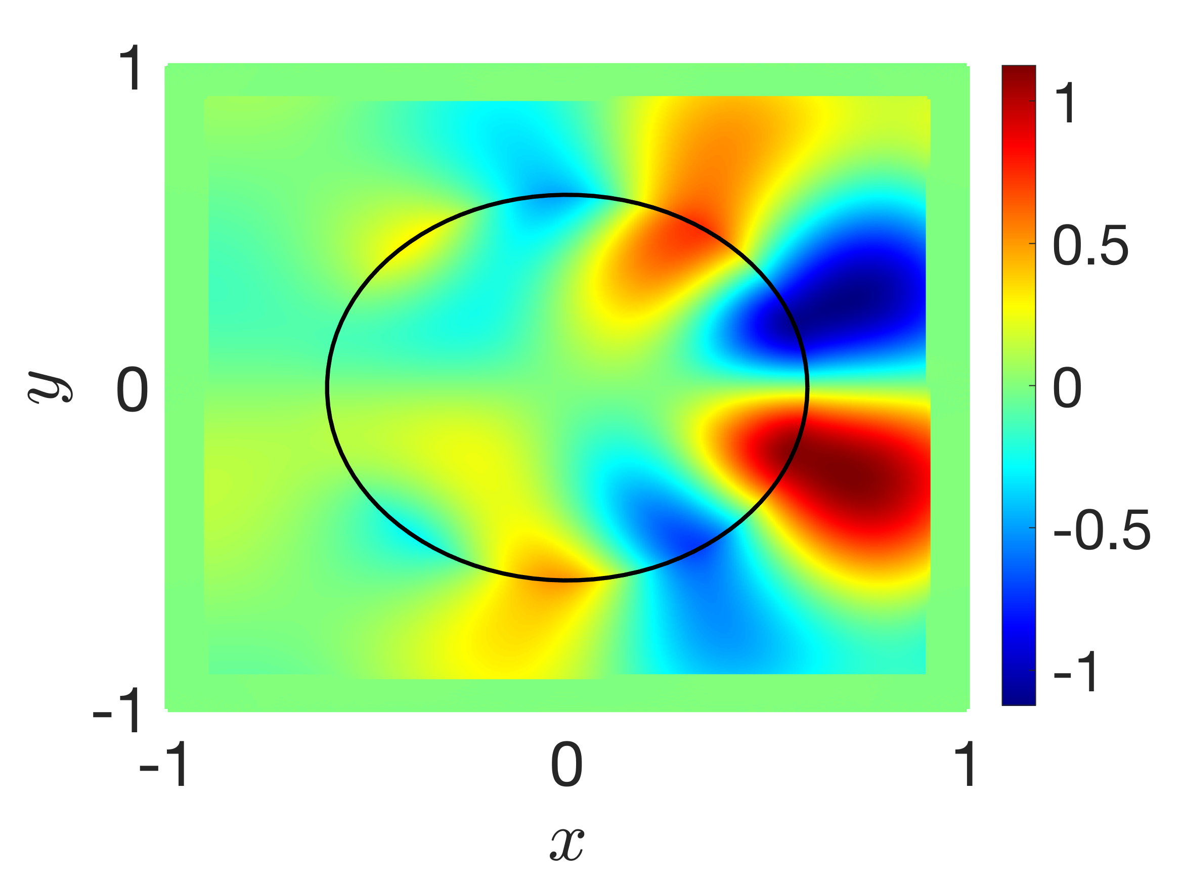
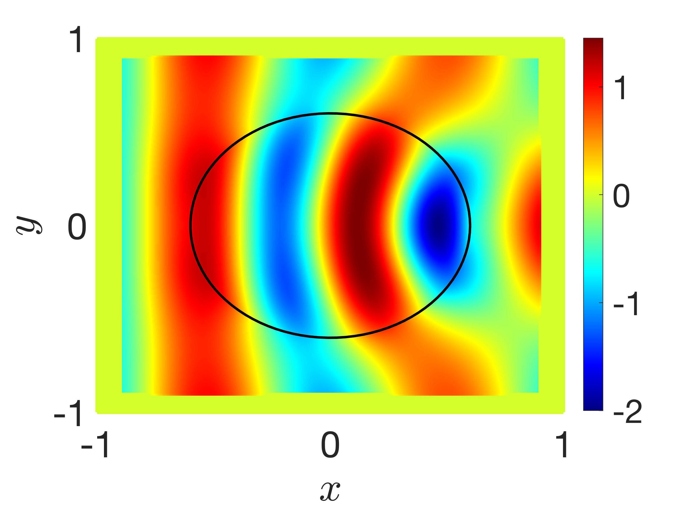
[5pt] [5pt]$H_{x}$ [5pt] $H_{y}$ [5pt] $E_{z}$ A

(a) a non-magnetic dielectric material ($\mu^{+}=\mu^{-}=1$, $\epsilon^{+}=1$ and $\epsilon^{-}=2.25$)

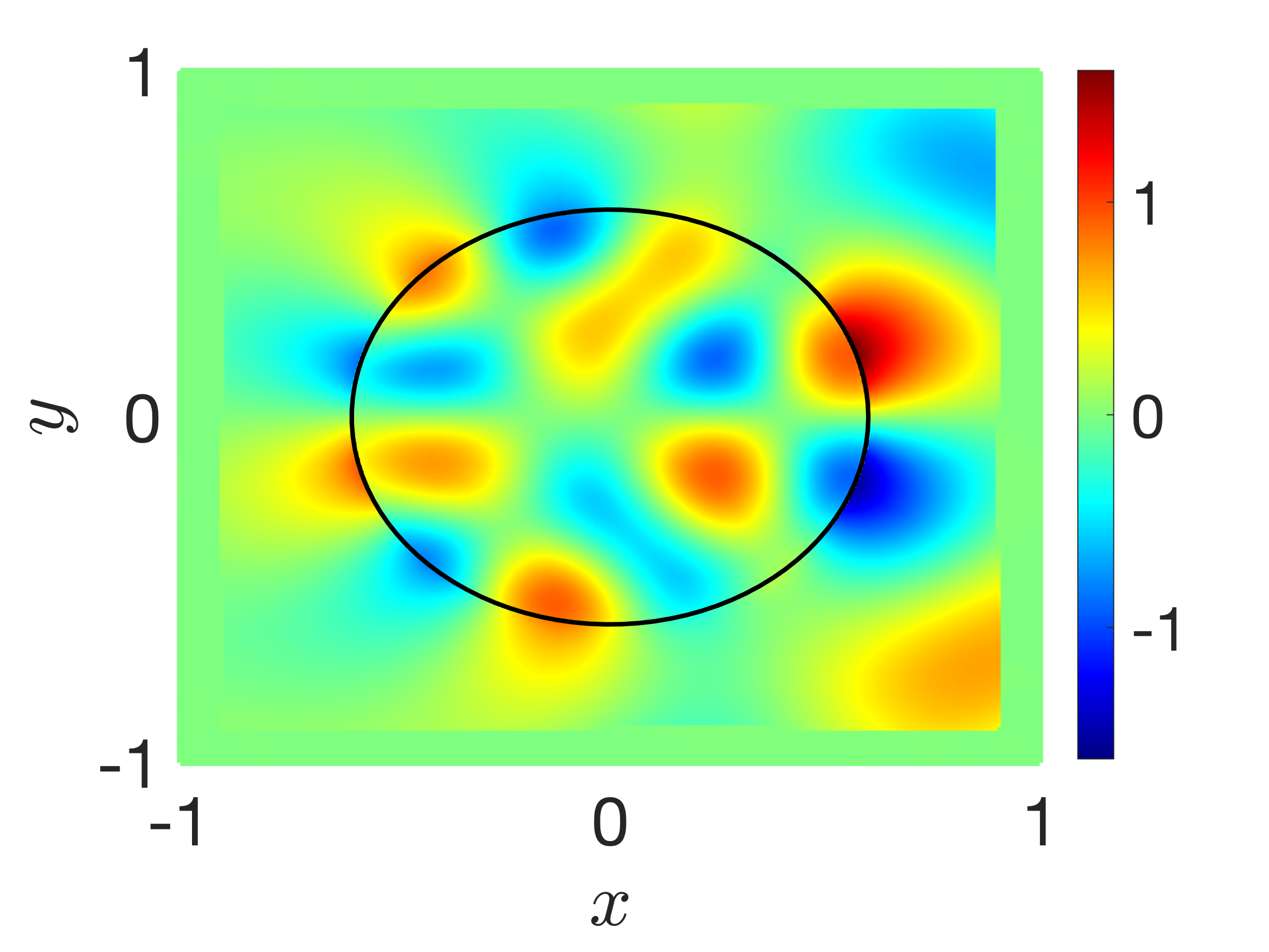
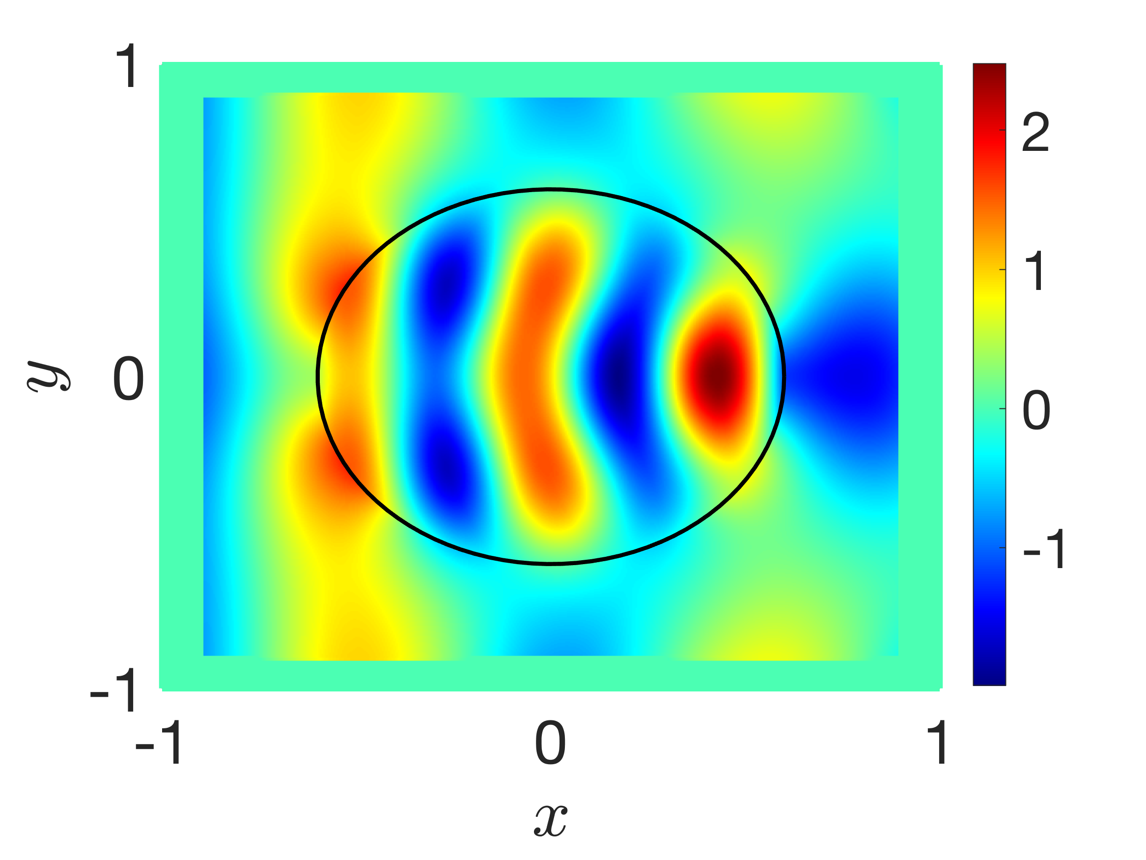
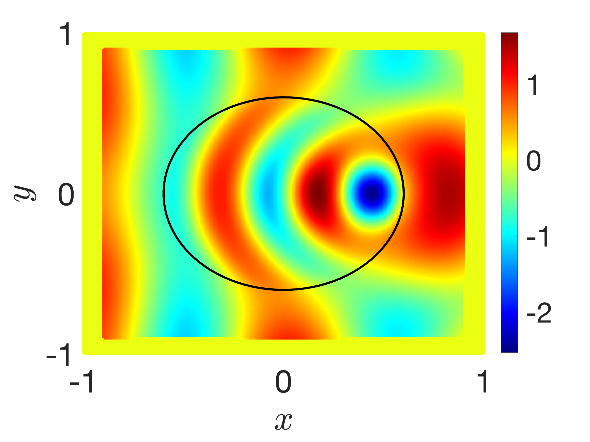
[5pt] [5pt]$H_{x}$ [5pt] $H_{y}$ [5pt] $E_{z}$ A

(b) a magnetic dielectric material ($\mu^{+}=1$, $\mu^{-}=2$, $\epsilon^{+}=1$ and $\epsilon^{-}=2.25$)

Figure 4: The components $H_{x}$, $H_{y}$ and $E_{z}$ with $h=\tfrac{1}{244}$ for scattering of a dielectric cylinder problems using the CFM-$4^{th}$ scheme. The computed electric field and magnetic field are shown respectively at $t=1$ and $t-\tfrac{\Delta t}{2}$. The interface is represented by the black line.

4.1.1 Verification of the Accuracy of Correction Functions

In this subsection, we assess the accuracy of the estimated correction functions coming from minimization problem (4) using high-order explicit jump conditions [10, 1]. Matched Interface and Boundary (MIB) based strategies use these conditions to construct high-order FDTD schemes. As mentioned in Remark 3.4, the correction function’s system of PDEs implicitly considers jump conditions coming from Maxwell’s equations (1). To provide numerical evidences of this claim, we compute the error on these jump conditions on all local patches using

$$\Big{(}\int\limits_{\Gamma\cap\Omega_{\Gamma}^{h}}\!\!\llbracket u(\mathbold{x},t_{f})\rrbracket^{2}\,\mathrm{d}S\Big{)}^{1/2},$$

where $\llbracket u(\mathbold{x},t_{f})\rrbracket$ is a given jump condition evaluated with approximated solutions of problem (4) at $t_{f}$. Afterward, the maximum error value on all local patches for a given order of jump conditions is taken and is denoted by $E_{i}$ for the $i^{th}$-order jump condition.

Although we do not have a theoretical result to characterize the convergence of high-order explicit jump conditions, one should expect a $(k+1-q)$ convergence for a $q^{th}$ order jump condition when $k$ degree polynomial approximations of correction functions are used. As an example, a third degree polynomial approximation should lead at least to a fourth, third, second and first order convergence for respectively the zeroth, first, second and third order jump conditions. It is recalled that second and third degree polynomial approximations of correction functions are used for respectively the CFM-Yee scheme and the CFM-$4^{th}$ scheme.

For a non-magnetic dielectric material, high-order jump conditions can be derived by using the continuity of time derivatives of electromagnetic fields on the interface [10] and are given by:

zeroth-order $$\,\,\left\{\begin{array}[]{l}\llbracket H_{x}\rrbracket=0,\\ \llbracket H_{y}\rrbracket=0,\\ \llbracket E_{z}\rrbracket=0,\\ \end{array}\right.\qquad\text{first-order}\,\,\left\{\begin{array}[]{l l}\llbracket\partial_{y}E_{z}\rrbracket=0,\\ \llbracket\partial_{x}E_{z}\rrbracket=0,\\ \big{\llbracket}\tfrac{1}{\epsilon}\,(\partial_{x}H_{y}-\partial_{y}H_{x})\big{\rrbracket}=0,\\ \end{array}\right.$$

second-order $$\,\,\left\{\begin{array}[]{l l}\big{\llbracket}\tfrac{1}{\epsilon}\,(\partial_{x}^{2}E_{z}-\partial_{y}^{2}E_{z})\big{\rrbracket}=0,\\ \big{\llbracket}\tfrac{1}{\epsilon}\,(\partial_{y}^{2}H_{x}-\partial_{xy}^{2}H_{y})\big{\rrbracket}=0,\\ \big{\llbracket}\tfrac{1}{\epsilon}\,(\partial_{x}^{2}H_{y}-\partial_{xy}^{2}H_{x})\big{\rrbracket}=0,\\ \end{array}\right.$$

third-order $$\,\,\left\{\begin{array}[]{l l}\big{\llbracket}\tfrac{1}{\epsilon}\,(\partial_{xxy}^{3}E_{z}+\partial_{y}^{3}E_{z})\big{\rrbracket}=0,\\ \big{\llbracket}\tfrac{1}{\epsilon}\,(\partial_{x}^{3}E_{z}+\partial_{xyy}^{3}E_{z})\big{\rrbracket}=0,\\ \big{\llbracket}\tfrac{1}{\epsilon^{2}}\,(\partial_{x}^{3}H_{y}+\partial_{xyy}^{3}H_{y}-\partial_{y}^{3}H_{x}-\partial_{xxy}^{3}H_{x})\big{\rrbracket}=0.\end{array}\right.$$

Figure 5 illustrates convergence plots of those jump conditions at $t_{f}=1$ for both schemes.

(a) zeroth-order jump conditions

(b) first-order jump conditions

(c) second-order jump conditions

(d) third-order jump conditions

Figure 5: Convergence plots of jump conditions for a scattering of a non-magnetic dielectric cylinder problem ($\mu^{+}=\mu^{-}=1$) using the proposed CFM-FDTD schemes.

We observe that the convergence order for all jump conditions is better than expected.

Let us now consider a magnetic dielectric material. Considering a point $\mathbold{p}=(x_{p},y_{p})$ on the interface $\Gamma$, one can define a local coordinate system based on the normal $\mathbold{n}$ and the tangent $\mathbold{\tau}$ to the interface at $\mathbold{p}$, and derive explicit jump conditions coming from Maxwell’s equations (1) [1]. In this local coordinate system, zeroth and first order jump conditions are given by

zeroth-order $$\,\,\left\{\begin{array}[]{l}\llbracket H_{\tau}\rrbracket=0,\\ \llbracket\mu\,H_{n}\rrbracket=0,\\ \llbracket E_{z}\rrbracket=0,\\ \end{array}\right.$$

first-order $$\,\,\left\{\begin{array}[]{l l}\llbracket\partial_{\tau}E_{z}\rrbracket=0,\\ \llbracket\tfrac{1}{\mu}\,\partial_{n}E_{z}\rrbracket=0,\\ \big{\llbracket}\partial_{n}(\mu\,H_{n})+\partial_{\tau}(\mu\,H_{\tau})\big{\rrbracket}=0,\\ \big{\llbracket}\partial_{n}(\mu\,H_{\tau})-\partial_{\tau}(\mu\,H_{n})-\partial_{t}(\mu\,\epsilon\,E_{z})\big{\rrbracket}=0.\end{array}\right.$$

(a) zeroth-order jump conditions

(b) first-order jump conditions

Figure 6: Convergence plots of jump conditions for a scattering of a magnetic dielectric cylinder problem with $\mu^{+}=1$ and $\mu^{-}=2$ using the proposed CFM-FDTD schemes.

Convergence plots of zeroth and first order jump conditions at $t_{f}=1$ are shown in Figure 6 for both schemes. A third-order convergence is observed for zeroth and first order jump conditions when the CFM-Yee scheme is used. As for the CFM-$4^{th}$ scheme, a fourth-order convergence is obtained for zeroth-order jump conditions while a three and a half order convergence is observed for first-order jump conditions. According to numerical results, approximations of correction functions coming from minimization problem (4) are consistent with high-order explicit jump conditions coming from Maxwell’s equation (1) and therefore are appropriate to correct FD approximations in the vicinity of the interface.

4.2 Problems with a Manufactured Solution

To our knowledge, there is no analytic solution for Maxwell’s interface problems with an arbitrary geometry of the interface. In order to verify the proposed numerical strategy, general interface conditions, given by

$$\hat{\mathbold{n}}\times\llbracket\mathbold{E}\rrbracket= \,\,\mathbold{a}(\mathbold{x},t)\quad\text{on }\Gamma\times I,$$ (6a)

$$\hat{\mathbold{n}}\times\llbracket\mathbold{H}\rrbracket= \,\,\mathbold{b}(\mathbold{x},t)\quad\text{on }\Gamma\times I,$$ (6b)

$$\hat{\mathbold{n}}\cdot\llbracket\epsilon(\mathbold{x})\,\mathbold{E}\rrbracket= \,\,c(\mathbold{x},t)\quad\text{on }\Gamma\times I,$$ (6c)

$$\hat{\mathbold{n}}\cdot\llbracket\mu(\mathbold{x})\,\mathbold{H}\rrbracket= \,\,d(\mathbold{x},t)\quad\text{on }\Gamma\times I,$$ (6d)

are considered. Hence, both tangential and normal components of electromagnetic fields can be discontinuous on the interface. Moreover, electromagnetic fields are at divergence-free in each subdomain, but not necessarily in the whole domain because of interface conditions (6c) and (6d). Source terms in each subdomain are given by $\mathbold{f}^{+}_{1}(\mathbold{x},t)$ and $\mathbold{f}^{-}_{1}(\mathbold{x},t)$ for Faraday’s law (1a), and by $\mathbold{f}^{+}_{2}(\mathbold{x},t)$ and $\mathbold{f}^{-}_{2}(\mathbold{x},t)$ for Ampère-Maxwell’s law (1b). It is worth mentioning that these source terms and interface conditions are not substantiated by physics. Nevertheless, they can be used to construct manufactured solutions that are needed to verify the proposed numerical strategy for arbitrary complex interfaces.

The domain is $\Omega=[0,1]\times[0,1]$ and the time interval is $I=[0,1]$. The physical parameters are given by $\mu^{+}=2$, $\epsilon^{+}=1$, $\mu^{-}=\sin(5\,\pi\,x\,y)+2$ and $\epsilon^{-}=2\,e^{x\,y}$. The magnetic permeability and the electrical permittivity have been chosen in such a way that electromagnetic fields are at divergence-free in each subdomain. The manufactured solutions are :

$$H_{x}^{+}= \,\,0.5\,\sin(2\,\pi\,x)\,\sin(2\,\pi\,y)\,\sin(2\,\pi\,t),$$

$$H_{y}^{+}= \,\,0.5\,\cos(2\,\pi\,x)\,\cos(2\,\pi\,y)\,\sin(2\,\pi\,t),$$

$$E_{z}^{+}= \,\,\sin(2\,\pi\,x)\,\cos(2\,\pi\,y)\,\cos(2\,\pi\,t)$$

in $\Omega^{+}$, and

$$H_{x}^{-}= \,\,-x\,e^{-x\,y}\,\sin(2\,\pi\,t),$$

$$H_{y}^{-}= \,\,y\,e^{-x\,y}\,\sin(2\,\pi\,t),$$

$$E_{z}^{-}= \,\,\sin(2\,\pi\,x\,y)\,\cos(2\,\pi\,t)$$

in $\Omega^{-}$. The associated source terms are $\mathbold{f}_{1}^{+}=0$, $f_{2}^{+}=0$ and

$$f_{1,x}^{-}= \,\,2\,\pi\,x\,\big{(}\cos(2\,\pi\,x\,y)-(\sin(5\,\pi\,x\,y)+2)\,e^{-x\,y}\big{)}\,\cos(2\,\pi\,t),$$

$$f_{1,y}^{-}= \,\,2\,\pi\,y\,\big{(}(\sin(5\,\pi\,x\,y)+2)\,e^{-x\,y}-\cos(2\,\pi\,x\,y)\big{)}\,\cos(2\,\pi\,t),$$

$$f_{2}^{-}= \,\,\big{(}(x^{2}+y^{2})\,e^{-x\,y}-4\,\pi\,e^{x\,y}\,\sin(2\,\pi\,x\,y)\big{)}\,\sin(2\,\pi\,t).$$

We consider geometries of the interface that are illustrated in Figure 7.

(a) circular

(b) 5-star

(c) 3-star

Figure 7: Different geometries of the interface.

Periodic boundary conditions are imposed on all $\partial\Omega$ for both CFM-FDTD schemes. The mesh grid size is $h=\Delta x=\Delta y$ and the time step is $\Delta t=\tfrac{h}{2}$ with $h\in\big{\{}\tfrac{1}{20},\tfrac{1}{28},\tfrac{1}{40},\tfrac{1}{52},\tfrac{1}{72},\tfrac{1}{96},\tfrac{1}{132},\tfrac{1}{180},\tfrac{1}{244},\tfrac{1}{336},\tfrac{1}{460}\big{\}}$. For local patches, we choose $\ell_{h}=\beta\,h$ with $\beta=8$ for the 5-star interface and $\beta=7$ for either the circular or 3-star interface. All other parameters are the same as in subsection 4.1. Figure 8 shows convergence plots of $\mathbold{U}=[H_{x},H_{y},E_{z}]^{T}$ for all geometries of the interface. We observe a second-order convergence in $L^{2}$-norm for the CFM-Yee scheme. As for the CFM-$4^{th}$ scheme, the expected order is not clearly observed for smaller mesh grid sizes. Since the error of $\mathbold{U}$ is already low for this scheme, this suggests a limitation due to the use of double-precision arithmetic and therefore a more accurate floating-point arithmetic should remedy this issue. Nevertheless, a global fourth-order convergence is observed using the $L^{2}$-norm. These results are in agreement with the theory.

(a) circle

(b) 5-star

(c) 3-star

Figure 8: Convergence plots for problems with a manufactured solution using the proposed CFM-FDTD schemes. It is recalled that $\mathbold{U}=[H_{x},H_{y},E_{z}]^{T}$.

Figure 9 illustrates the computed solutions for different geometries of the interface. One can observe that there is no spurious oscillation in the vicinity of the interface.

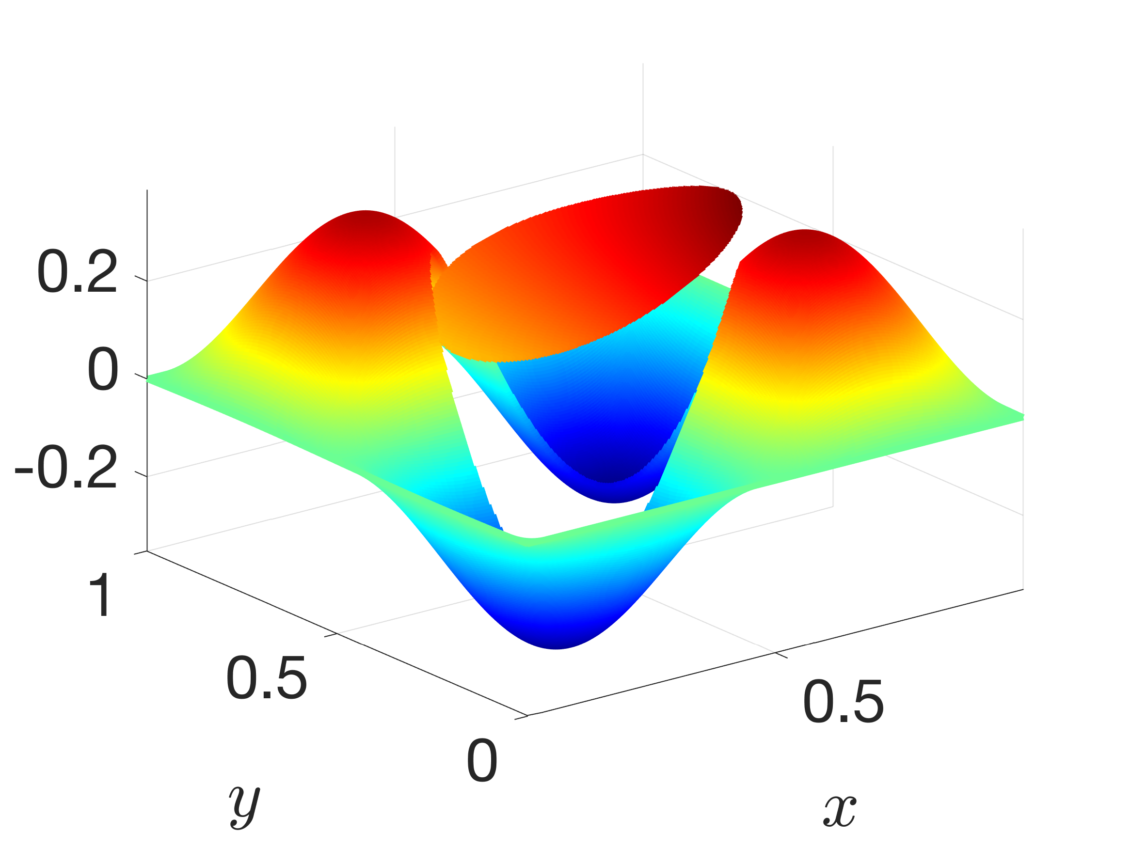
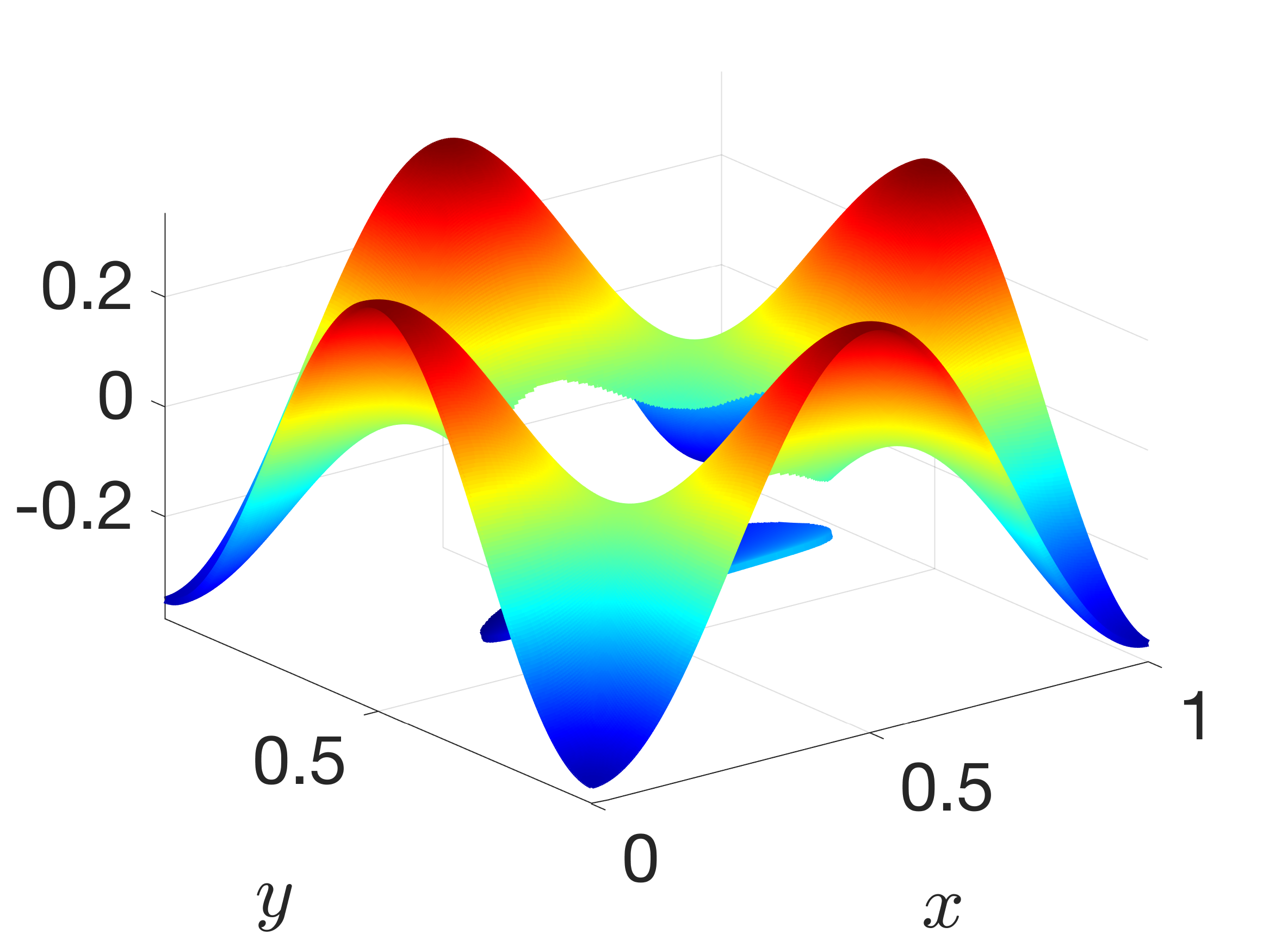
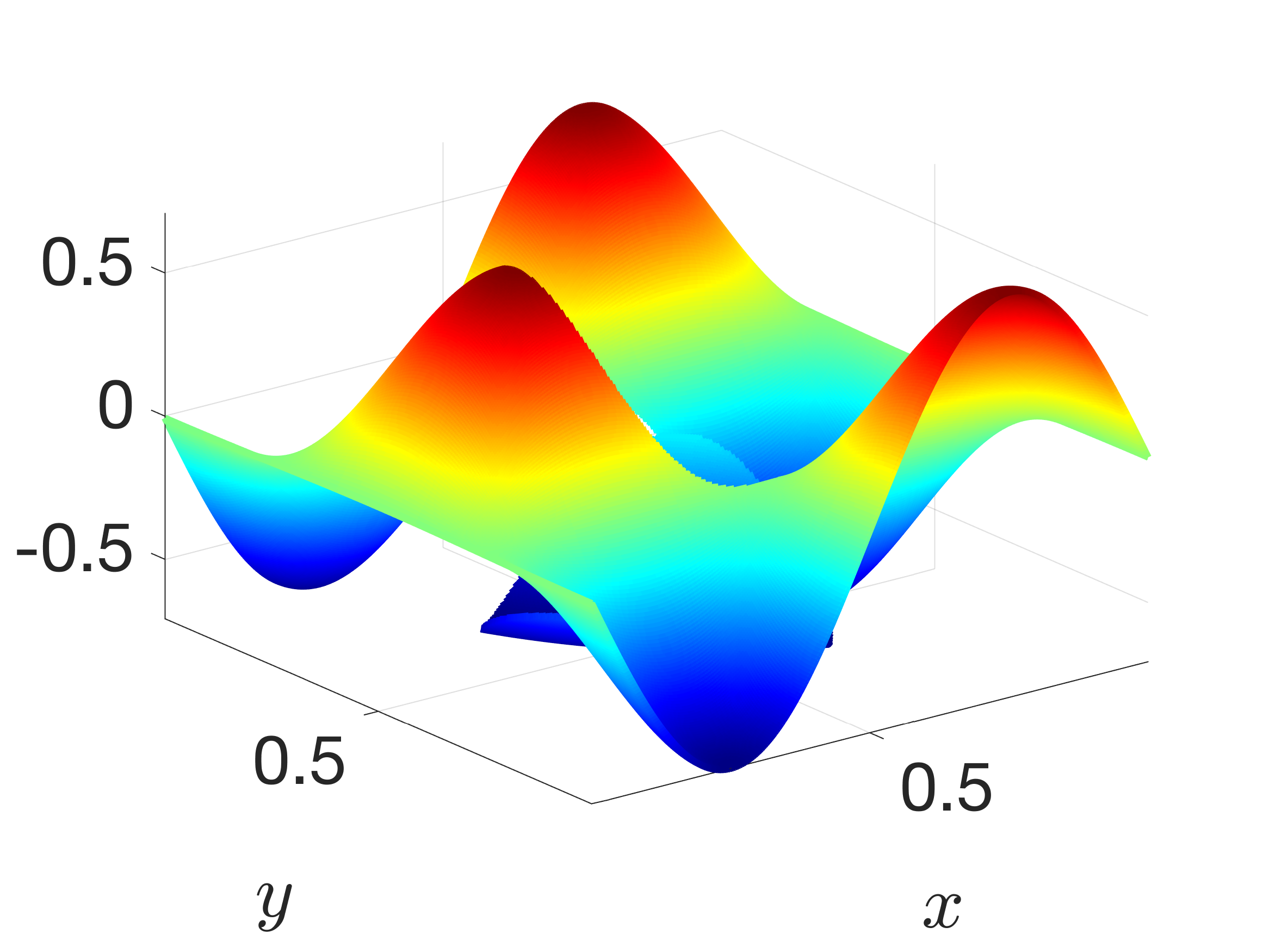
[5pt] [5pt]$H_{x}$ [5pt] $H_{y}$ [5pt] $E_{z}$ A

(a) circular

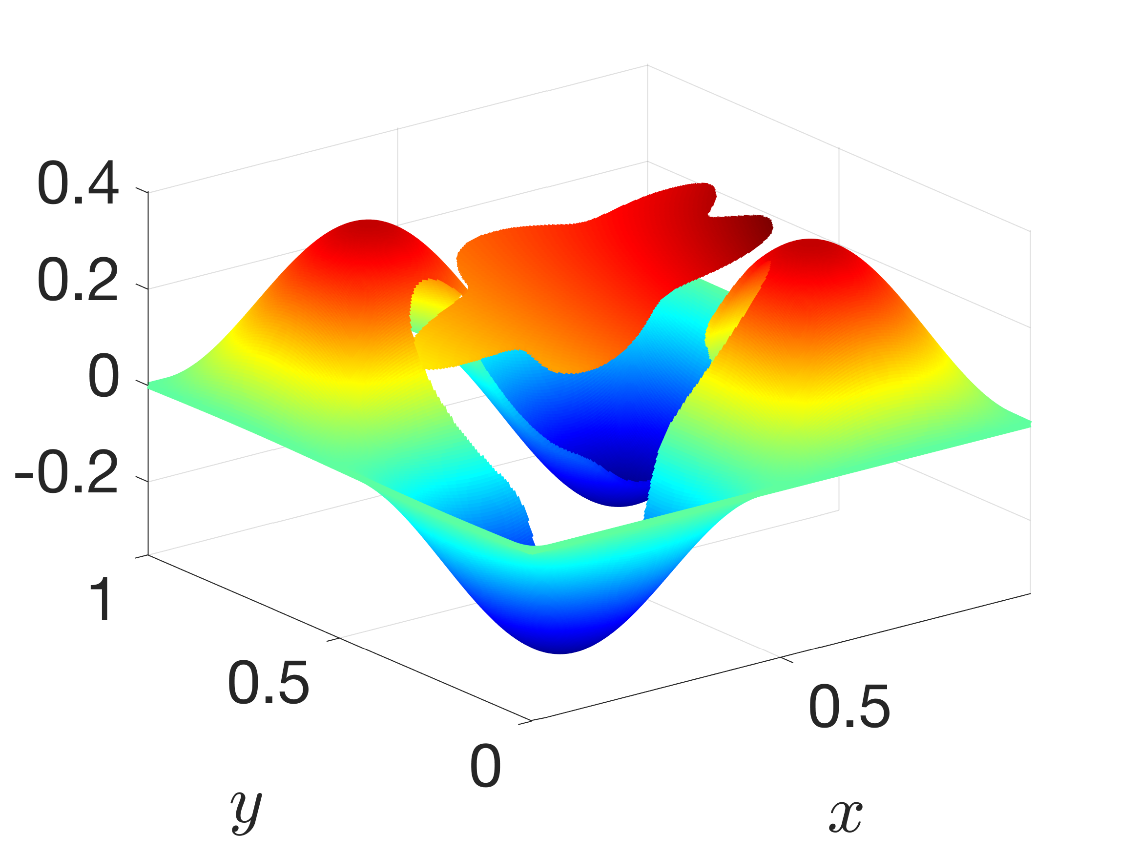
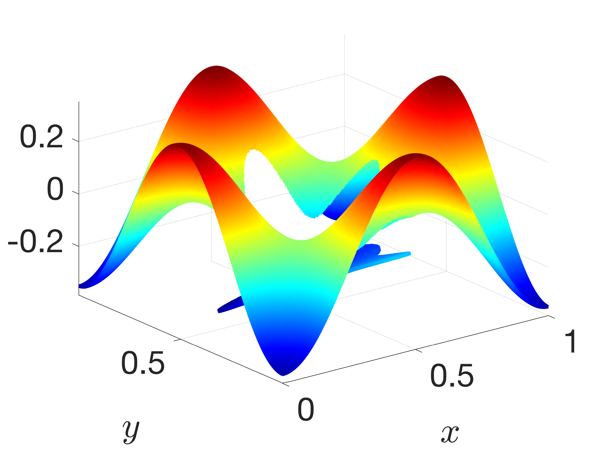
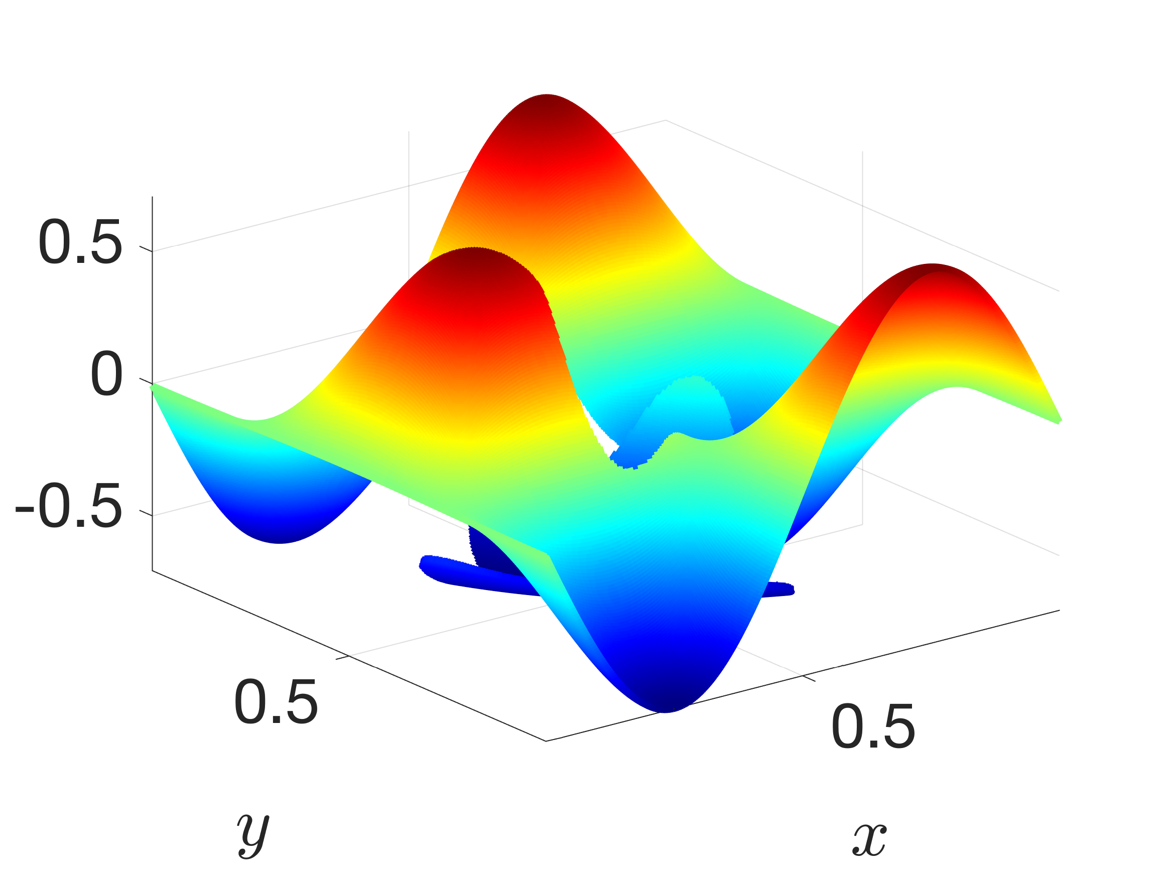
[5pt] [5pt]$H_{x}$ [5pt] $H_{y}$ [5pt] $E_{z}$ A

(b) 5-star

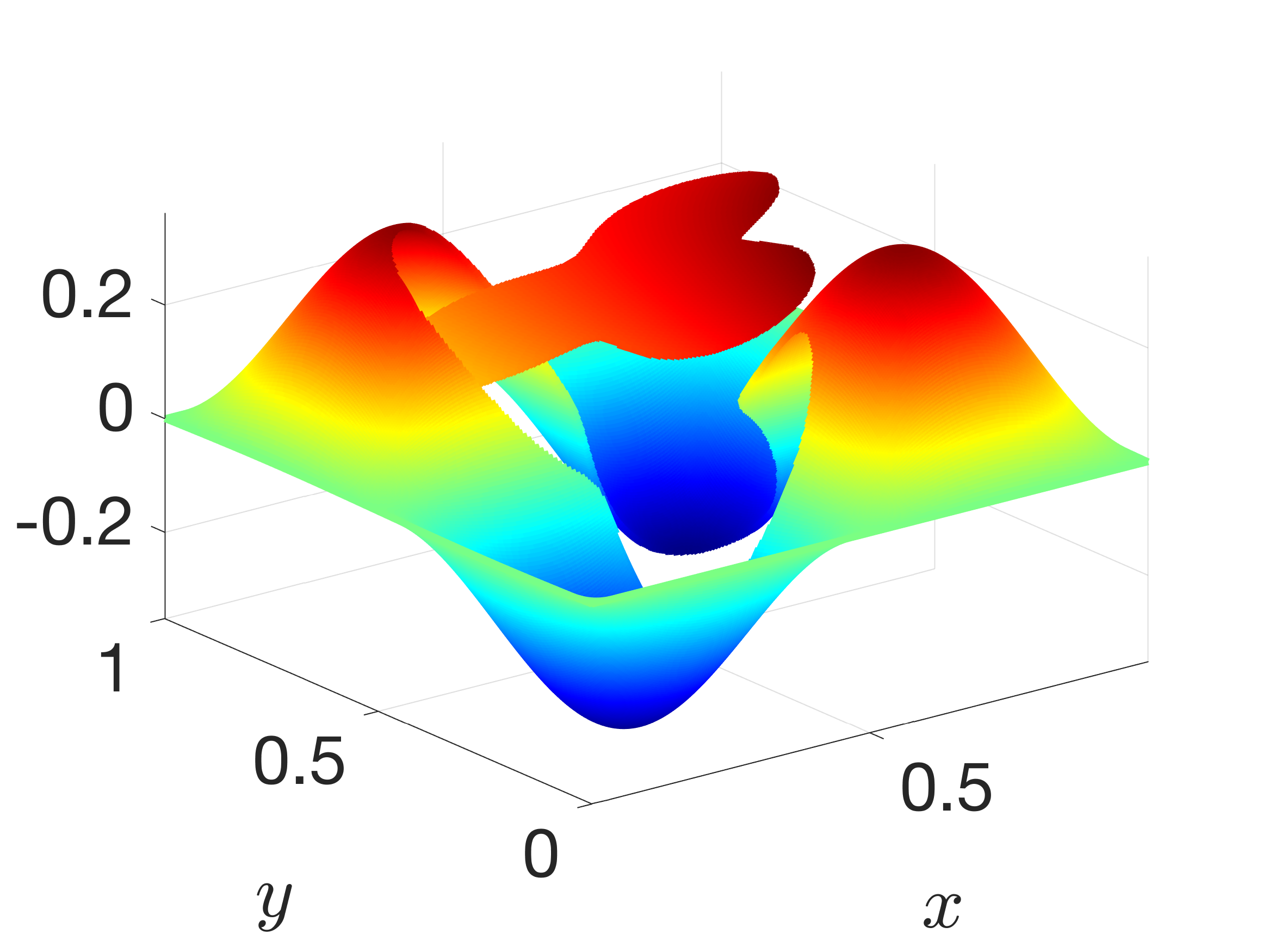
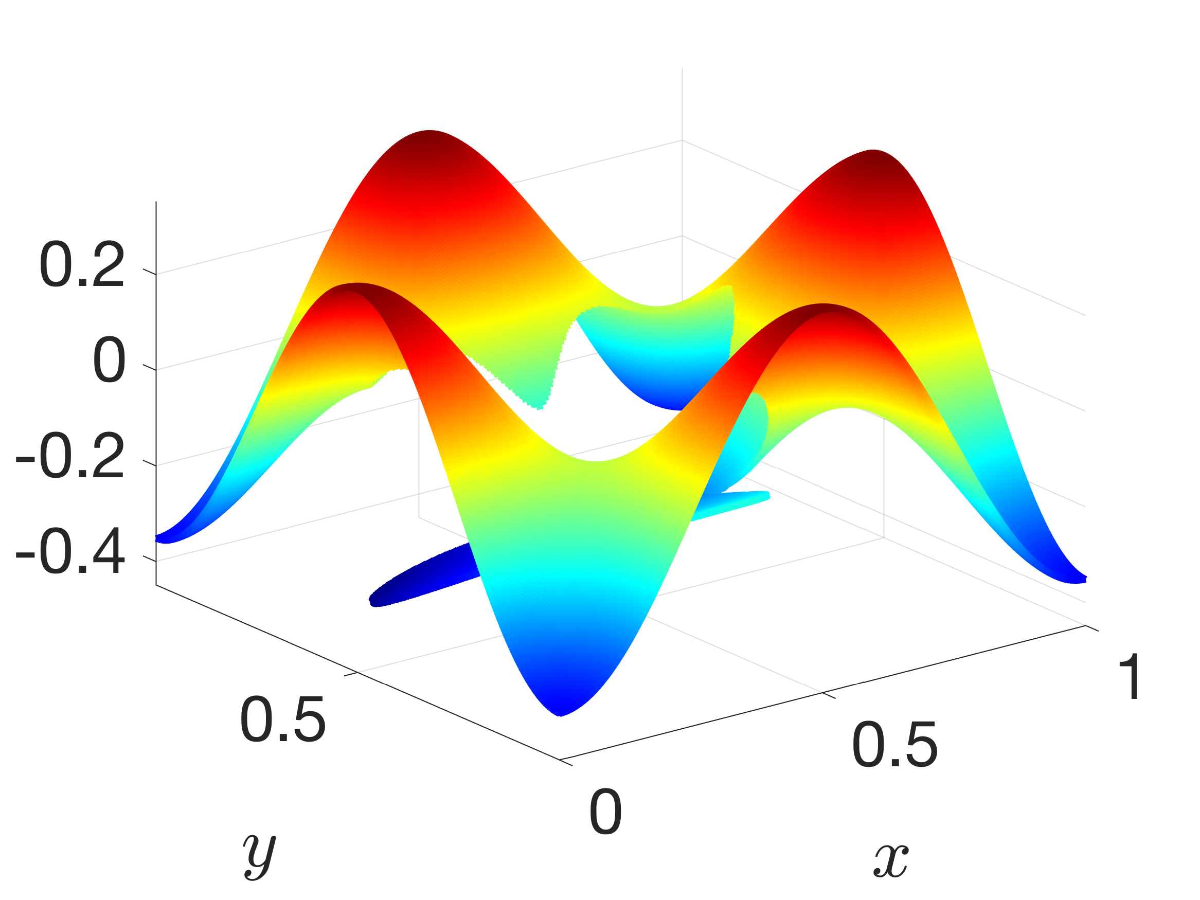
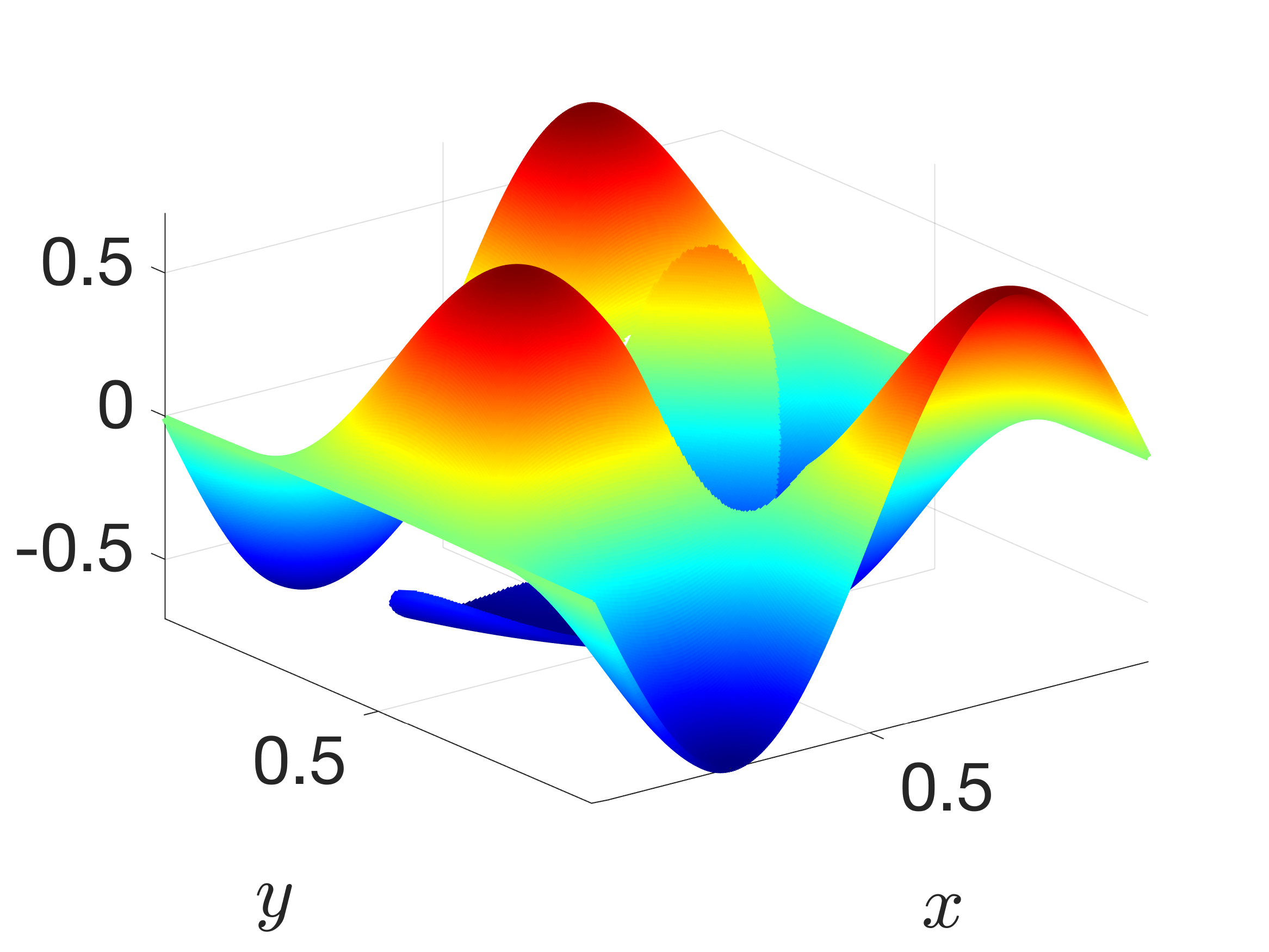
[5pt] [5pt]$H_{x}$ [5pt] $H_{y}$ [5pt] $E_{z}$ A

(c) 3-star

Figure 9: The components $H_{x}$, $H_{y}$ and $E_{z}$ with $h=\tfrac{1}{336}$ for problems with a manufactured solution using the CFM-Yee scheme. The computed electric field and magnetic field are shown respectively at $t=0.625$ and $t-\frac{\Delta t}{2}$.

4.3 Stability Investigation : Long-Time Simulations

As mentioned in Remark 3.5, a rigorous stability analysis of CFM-FDTD schemes is out of reach for the moment. In this short subsection, we therefore provide some numerical evidences on the stability of CFM-FDTD schemes for a sufficiently small value of the penalization coefficient $c_{f}$. We consider scattering of a dielectric cylinder problems, and a problem with a manufactured solution and a 3-star interface. We use the CFM-Yee and the CFM-4^th scheme. For both CFM-FDTD schemes, the parameters remain the same as previously described. However, we consider a larger time interval, given by $I=[0,25]$.

(a) CFM-Yee

(b) CFM-4^th

Figure 10: Evolution of the error in $L^{2}$-norm of $\mathbold{U}=[H_{x},H_{y},E_{z}]^{T}$ for a scattering of a dielectric cylinder problem with $\mu^{+}=\mu^{-}=1$ using the proposed CFM-FDTD schemes. The mesh grid size $\tfrac{1}{20}$, $\tfrac{1}{40}$ and $\tfrac{1}{80}$ correspond to respectively the black line, dotted blue line and dash-dotted magenta line.

(a) CFM-Yee

(b) CFM-4^th

Figure 11: Evolution of the error in $L^{2}$-norm of $\mathbold{U}=[H_{x},H_{y},E_{z}]^{T}$ for a scattering of a dielectric cylinder problem with $\mu^{+}=1$ and $\mu^{-}=2$ using the proposed CFM-FDTD schemes. The mesh grid size $\tfrac{1}{20}$, $\tfrac{1}{40}$ and $\tfrac{1}{80}$ correspond to respectively the black line, dotted blue line and dash-dotted magenta line.

(a) CFM-Yee

(b) CFM-4^th

Figure 12: Evolution of the error in $L^{2}$-norm of $\mathbold{U}=[H_{x},H_{y},E_{z}]^{T}$ for a problem with a manufactured solution using a 3-star interface and the proposed CFM-FDTD schemes. The mesh grid size $\tfrac{1}{20}$, $\tfrac{1}{40}$ and $\tfrac{1}{80}$ correspond to respectively the black line, dotted blue line and dash-dotted magenta line.

Figure 10, Figure 11 and Figure 12 illustrate the evolution of the error in $L^{2}$-norm of $\mathbold{U}=[H_{x},H_{y},E_{z}]^{T}$ for respectively a non-magnetic dielectric cylinder problem, a magnetic dielectric cylinder problem and a problem with a manufactured solution. In all cases, numerical results suggest that the proposed CFM-FDTD schemes are stable.

5 Conclusions

In this work, we presented high-order FDTD schemes based on the Correction Function Method. The system of PDEs needed for the CFM was derived using Maxwell’s equations with interface conditions. The minimization problem based on a functional that is a square measure of the error associated with the correction function’s system of PDEs was also presented and solved. Numerical examples showed that numerical solutions coming from CFM-FDTD schemes were captured without spurious oscillation while exhibiting high-order convergence. Moreover, the accuracy of correction functions has been verified using high-order explicit jump conditions. This showed that high-order jump conditions are implicitly enforced in the functional to minimize and therefore need not be provided explicitly. Problems with a manufactured solution have shown that the proposed numerical strategy can handle various geometries of the interface without significantly increasing the complexity of the method. Despite a lack of a rigorous stability analysis, long-time simulations have been performed and provided numerical evidences of the stability of CFM-FDTD schemes. Future work will focus on the theoretical aspect of the CFM as well as an extension of this strategy to 3-D problems.

References

References

- [1] Y. Zhang, D. D. Nguyen, K. Du, J. Xu, S. Zhao, Time-domain numerical solutions of Maxwell interface problems with discontinuous electromagnetic waves, Adv. Appl. Math. Mech. 8 (2016) 353–385.
- [2] J. S. Hesthaven, High-order accurate methods in time-domain computational electromagnetics: a review, Adv. Imag. Electron Phys. 127 (2003) 59–123.
- [3] R. J. LeVeque, Z. Li, The immersed interface method for elliptic equations with discontinuous coefficients and singular sources, SIAM J. Num. Anal. 31 (4) (1994) 1019–1044.
- [4] R. P. Fedkiw, T. Aslam, B. Merriman, S. Osher, A non-oscillatory eulerian approach to interfaces in multimaterial flows (the ghost fluid method), J. Comput. Phys. 152 (1999) 457–492.
- [5] A. N. Marques, J.-C. Nave, R. R. Rosales, A correction function method for Poisson problems with interface jump conditions, J. Comput. Phys. 230 (2011) 7567–7597.
- [6] K. S. Yee, Numerical solution of initial boundary value problems involving Maxwell’s equations in isotropic media, IEEE Trans. Antennas Propag. 14 (3) (1966) 302–307.
- [7] A. Ditkowski, K. Dridi, J. S. Hesthaven, Convergent cartesian grid methods for Maxwell equations in complex geometries, J. Comput. Phys. 170 (2001) 39–80.
- [8] K. Dridi, J. S. Hesthaven, A. Ditkowski, Staircase-free finite-difference time-domain formulation for general materials in complex geometries, IEEE Trans. Antennas Propag. 49 (5) (2001) 749–756.
- [9] W. Cai, S. Deng, An upwinding embedded boundary method for Maxwell’s equations in media with material interfaces: 2D case, J. Comput. Phys. 190 (2003) 159–183.
- [10] S. Zhao, G. W. Wei, High-order FDTD methods via derivative matching for Maxwell’s equations with material interfaces, J. Comput. Phys. 200 (2004) 60–103.
- [11] D. D. Nguyen, S. Zhao, A new high order dispersive FDTD method for Drude material with complex interfaces, J. Comput. Appl. Math. 289 (2015) 1–14.
- [12] D. D. Nguyen, S. Zhao, A second order dispersive FDTD algorithm for transverse electric Maxwell’s equations with complex interfaces, Comput. Math. Appl. 71 (2016) 1010–1035.
- [13] S. Yu, Y. Zhou, G. W. Wei, Matched interface and boundary (MIB) method for elliptic problems with sharp-edged interfaces, J. Comput. Phys. 224 (2007) 729–756.
- [14] D. S. Abraham, D. D. Giannacopoulos, A parallel implementation of the correction function method for Poisson’s equation with immersed surface charges, IEEE Trans. Magn. 53 (6).
- [15] A. N. Marques, A correction function method to solve incompressible fluid flows to high accuracy with immersed geometries, Ph.D. thesis, Massachusetts Institute of Technology (2012).
- [16] A. N. Marques, J.-C. Nave, R. R. Rosales, High order solution of Poisson problems with piecewise constant coefficients and interface jumps, J. Comput. Phys. 335 (2017) 497–515.
- [17] A. N. Marques, J.-C. Nave, R. R. Rosales, Imposing jump conditions on nonconforming interfaces for the correction function method: a least squares approach, J. Comput. Phys. 397 (2019) 108869.
- [18] D. S. Abraham, A. N. Marques, J.-C. Nave, A correction function method for the wave equation with interface jump conditions, J. Comput. Phys. 353 (2018) 281–299.
- [19] Y. M. Law, J.-C. Nave, FDTD schemes for maxwell’s equations with embedded perfect electric conductors based on the correction function method, J. Comput. Phys., submitted for publication, arxiv:1909.10570.
- [20] Y.-M. Law, A. N. Marques, J.-C. Nave, Treatment of complex interfaces for Maxwell’s equations with continuous coefficients using the correction function method, J. Sci. Comput. 82 (3) (2020) 56.
- [21] B. Cockburn, F. Li, C.-W. Shu, Locally divergence-free discontinuous Galerkin methods for the Maxwell equations, J. Comput. Phys. 194 (2) (2004) 588–610.
- [22] M. Ghrist, B. Fornberg, T. A. Driscoll, Staggered time integrators for wave equations, SIAM J. Numer. Anal. 38 (2000) 718–741.
- [23] A. Taflove, Computational electrodynamics : the finite difference time-domain method, Artech House, 1995.
- [24] J. Bezanson, A. Edelman, S. Karpinski, V. B. Shah, Julia: a fresh approach to numerical computing, SIAM Rev. 59 (2017) 65–98.