Assortativity measures for weighted and directed networks

Abstract

Assortativity measures the tendency of a vertex in a network being connected by other vertexes with respect to some vertex-specific features. Classical assortativity coefficients are defined for unweighted and undirected networks with respect to vertex degree. We propose a class of assortativity coefficients that capture the assortative characteristics and structure of weighted and directed networks more precisely. The vertex-to-vertex strength correlation is used as an example, but the proposed measure can be applied to any pair of vertex-specific features. The effectiveness of the proposed measure is assessed through extensive simulations based on prevalent random network models in comparison with existing assortativity measures. In application World Input-Ouput Networks, the new measures reveal interesting insights that would not be obtained by using existing ones. An implementation is publicly available in a R package wdnet.

1 Introduction

In traditional network analysis, assortativity or assortative mixing (Newman, 2002) is a measure assessing the preference of a vertex being connected (by edges) with other vertexes in a network. The measure reflects the principle of homophily (McPherson et al., 2001)—the tendency of the entities to be associated with similar partners in a social network. The primitive assortativity measure proposed by Newman (2002) was defined to study the tendency of connections between nodes based on their degrees, which is why it is also called degree-degree correlation (van der Hofstad and Litvak, 2014). Assortativity can be defined on any vertex feature, although vertex degree is the most popular (Newman, 2002, 2003). The measure has many applications in different types of networks; for example, the collaborative network among the authors on the arXiv preprint platform (Catanzaro et al., 2004), the transaction network of country-sectors in the global economy (Cerina et al., 2015), the bilateral trade relationships among the countries in the International Trade Network (Abbate et al., 2018), and the associations among the geographical regions in an earthquake network (Abe and Suzuki, 2006).

Classical assortativity measures and their extensions are defined for unweighted, undirected networks. Piraveenan et al. (2008) introduced a vertex-based local assortativity measure quantifying the contribution to the global assortativity of the network by each vertex. van Mieghem et al. (2010) reformulated the measure of Newman (2002), which led to a degree-preserving rewiring algorithm for unweighted and undirected networks. Mathematically, Newman’s assortativity measure is analogous to the sample Pearson correlation coefficient in statistics. In the context of networks, this measure has a limitation that its magnitude depends on the network size (Dorogovtsev et al., 2010; Raschke et al., 2010). Litvak and van der Hofstad (2013) gave examples of generative networks whose assotativity coefficients are expected to be negative but Newman’s measure gives zero when the network sizes are large. This motivated Litvak and van der Hofstad (2013) to propose a rank-based assortativity measure analogous to the sample Spearman correlation coefficient, which partially overcomes the limitation. All the definitions mentioned so far only involve directly connected vertices. To account for the possibility of a strong association induced by a multi-step path between two vertices, Arcagni et al. (2017) introduced a series of high-order assortativity measures quantifying the association among the vertices through a few network properties, including paths, shortest paths, and random walks with fixed length.

When a network is weighted (i.e., non-unit weights are assigned to the edges), it is necessary to extend Newman’s assortativity appropriately to a weighted version. Ignoring the weights may lead to misspecification of the network model and biased inferences. Leung and Chau (2007) introduced a weighted assortativity coefficient for weighted networks, where each edge weight is interpreted as the intensity of the interaction between the ending vertexes. Specifically, they used the world-wide airport network and the scientist collaboration network (Barrat et al., 2004) as examples. More recently, Arcagni et al. (2019) extended the concept of high-order assortativities (Arcagni et al., 2017) to a class of assortativity measures applicable to weighted networks by building a connection between assortativity and centrality (Newman, 2010) via edge weights. The new class includes four cases, where cases 1 and 3 were respectively generalized from the counterparts given in Newman (2002) and Leung and Chau (2007), and cases 2 and 4 were further extended from cases 1 and 3, respectively.

When edge direction needs to be accounted, assortativity is expected to distinguish the features of source and target vertices. Such features can be either in-degree or out-degree. Newman (2003) extended the classical assortativity (Newman, 2002) to an out-in assortativity. In the context of directed biological networks, Piraveenan et al. (2012) proposed out-out and in-in assortativity measures, and named them, respectively, out-assortativity and in-assortativity. The out-assortativity and in-assortativity of the studied directed biological networks generally higher than out-in assortativity coefficient. Foster et al. (2010) introduced four kinds of degree-degree correlations, $\left(\rm out,in\right)$, $\left(\rm out,out\right)$, $\left(\rm in,out\right)$ and $\left(\rm in,in\right)$, where the $\left(\rm out,in\right)$ correlation is equivalent to that in Newman (2003), and the $\left(\rm out,out\right)$ and $\left(\rm in,in\right)$ correlations are respectively equivalent to the out- and in-assortativity in Piraveenan et al. (2012). Foster et al. (2010) showed that some real networks (e.g., food webs) displayed assortative and disassortative mixing simultaneously.

Many networks in practice are both directed and weighted. For instance, consider the World Input-Output Network (WION) defined by a World Input-Output Table (WIOT, Timmer et al., 2015). Each vertex in a WION represents a region-sector, i.e., a sector in a country, region, or territory. A directed edge represents the monetary amount of the transactions from its source region-sector to its target region-sector, with the amount defining the edge weight. Despite the applications of network modeling tools to WIONs (e.g., Cerina et al., 2015), there is rather limited work on assortativity measures for weighted and directed networks in the literature. The classical assortativity measure cannot appropriately quantify the assortativity in a WION. The structure of a WION provides a vehicle to study any feature between the source region-sectors and target region-sectors, which could provide insights into the assortative or disassortative mixing beyond what has been typically studied.

We summarize the three major contributions of the present paper. First, we propose a class of assortativity measures for weighted and directed networks. The proposed measures can be used to analyze the correlation structure of both network-based properties and vertex-specific features; hence, they are general. Second, the necessity of incorporating weight and direction is illustrated via extensive numerical studies on widespread network models. We assert that edge weight is sine qua non of the assortativity of weighted networks, while ignoring it in the computation would fail to capture network features and possibly lead to incorrect inference. Finally, we apply the proposed assortativity measures to the annual series of WIONs from 2000 to 2004 to investigate the association among various region-sectors.

2 Weighted and Directed Assortativity Coefficients

Let $G(V,E)$ be a network consisting of a set of vertices $V$ and a set of edges $E$. The cardinalities of $V$ and $E$, respectively denoted by $|V|$ and $|E|$, are called the order and the size of $G$. For any $i\neq j\in V$, let $e_{ij}$ denote a directed edge (excluding self-loop) from vertex $i$ to $j$. We use $\bm{A}^{(G)}:=(a_{ij})_{|V|\times|V|}$ to represent the adjacency matrix of an unweighted network $G(V,E)$ such that $a_{ij}=1$ if $e_{ij}\in E$ and $a_{ij}=0$, otherwise. When $G(V,E)$ is weighted, we use $\bm{W}^{(G)}:=(w_{ij})_{|V|\times|V|}$ to represent the weighted analogue of $\bm{A}^{(G)}$. That is, $w_{ij}>0$ is the weight of $e_{ij}$ if $e_{ij}\in E$; $w_{ij}=0$, otherwise. Apparently, $\bm{A}^{(G)}$ and $\bm{W}^{(G)}$ are identical for unweighted networks. For ease of notation, we suppress the superscripts of $\bm{A}^{(G)}$ and $\bm{W}^{(G)}$ in the sequel.

The degree of a vertex in an undirected network is the number of edges incident to it. In directed networks, the out-degree and in-degree of a vertex are the number of edges emanating from and pointing to it, respectively. We use $d_{i}$, $d^{\,(\rm in)}_{i}$ and $d^{\,(\rm out)}_{i}$ for the degree, the in-degree, and the out-degree of vertex $i$, respectively. When edge weights are present, we define out-strength and in-strength of a vertex as the total weights of the edges emanating from and pointing to it. The total strength (or simply strength) of a vertex is the sum of its in-strength and out-strength. The strength, in-strength, and out-strength of vertex $i$ are respectively denoted by $s_{i}$, $s^{(\rm in)}_{i}$ and $s^{(\rm out)}_{i}$.

In classical network analysis, assortativity is usually referred to a degree-degree correlation. In general, assortativity can be used as a tool measuring the association between any pair of vertex features. Let $X$ and $Y$ be two quantitative features for all the vertices in a weighted and directed network $G(V,E)$. Let $(X_{i},Y_{i})$ be the two features for each vertex $i\in V$. Our weighted and directed assortativity measure based on the sample Pearson correlation coefficient is defined as

$$\rho_{X,Y}(G)=\frac{\sum_{i,j\in V}w_{ij}(X_{i}-\bar{X}_{\rm sou})(Y_{j}-\bar{Y}_{\rm tar})}{W\sigma_{X}\sigma_{Y}},$$ (1)

where $W:=\sum_{i,j\in V}w_{ij}$ is the sum of edge weights, $\bar{X}_{\rm sou}$ is the average of feature $X$ based on source vertices, $\bar{X}_{\rm sou}=\sum_{i,k\in V}w_{ik}X_{i}/W$ is the average of feature $X$ based on source vertices, $\bar{Y}_{\rm tar}=\sum_{k,j\in V}w_{kj}Y_{j}/W$ is the average of feature $Y$ based on target vertices, $\sigma_{X}=\sqrt{\sum_{i,k\in V}w_{ik}(X_{i}-\bar{X}_{\rm sou})^{2}/W}$ and $\sigma_{Y}=\sqrt{\sum_{k,j\in V}w_{kj}(Y_{j}-\bar{Y}_{\rm tar})^{2}/W}$ are the associated standard deviations, respectively. The two features $X$ and $Y$ could be the same feature such as the total strength.

Specifically, we look into strength-strength correlations by incorporating edge weights with the four (directed but unweighted) assortativity measures proposed by Foster et al. (2010). For each edge, let $\alpha,\beta\in\left\{{\rm in},{\rm out}\right\}$ index the strength type of the vertices at the two ends. We accordingly have four kinds of extended assortativity measures for a weighted and directed network $G$, denoted $\rho_{\alpha,\beta}(G)$. Note that Equation (1) is well defined for any $w_{ij}\in\mathbb{R}^{+}$ for $i,j\in V$. In the special case where all edge weights $w_{ij}$’s are positive integers, each edge can be regarded as a multi-edge, structurally equivalent to $w$ edges with unit weight.

According to Equation (1), we define the $(\alpha,\beta)$-type assortativity coefficient of a weighted and directed network $G(V,E)$ as follows:

$$\rho_{\alpha,\beta}(G)=\frac{\sum_{i,j\in V}w_{ij}\left[\left(s_{i}^{(\alpha)}-\bar{s}_{\rm sou}^{\,(\alpha)}\right)\left(s_{j}^{(\beta)}-\bar{s}_{\rm tar}^{\,(\beta)}\right)\right]}{W\sigma_{\rm sou}^{(\alpha)}\sigma_{\rm tar}^{(\beta)}},$$ (2)

where $s_{i}^{(\alpha)}$ is the $\alpha$-type strength of the source vertex $i$,

$$\bar{s}_{\rm sou}^{\,(\alpha)}=\frac{\sum_{i,j\in V}w_{ij}s_{i}^{\,(\alpha)}}{W}=\frac{\sum_{i\in V}s^{(\rm out)}_{i}s_{i}^{(\alpha)}}{W}$$

is the weighted mean of the $\alpha$-type strengths of the source vertices and

$$\sigma_{\rm sou}^{(\alpha)}=\sqrt{\frac{\sum_{i,k\in V}w_{ik}\left(s_{i}^{(\alpha)}-\bar{s}_{\rm sou}^{\,(\alpha)}\right)^{2}}{W}}=\sqrt{\frac{\sum_{i\in V}s^{(\rm out)}_{i}\left(s_{i}^{(\alpha)}-\bar{s}_{\rm sou}^{\,(\alpha)}\right)^{2}}{W}}$$

is the associated weighted standard deviation. The counterparts $s_{j}^{(\beta)}$, $\bar{s}_{\rm tar}^{\,(\beta)}$ and $\sigma_{\rm tar}^{(\beta)}$ are defined analogously for the target vertex $j$, where the weights in the weighted mean and the weighted standard deviation are replaced with $s^{(\rm in)}_{j}$. An illustrative example of the proposed assortativity measures is given in Appendix A.

The value of $\rho_{\alpha,\beta}(G)$ is bounded between $-1$ and $1$. The sign indicates the direction of the assortativity. A larger magnitude indicates a higher assortativity between the vertices with large $\alpha$-type strength and those with $\beta$-type strength in $G$. The boundary values are attainable in some extreme cases. Several examples are presented in Appendix C. The definition of $\rho_{\alpha,\beta}(G)$ is a sample measure, which should be fluctuating around the population measure of the network model that generates the observed network. When $G$ is completely random, for instance, as generated from the Erdös–Rényi random network model (Erdös and Rényi, 1959), the population measure should be zero as there is no tendency of vertex connection. The coefficient will be close to zero when the network size is sufficiently large.

The proposed assortativity coefficient in Equation (2) is well-defined for networks that are unweighted, undirected or both. Specifically, it is equivalent to that given in Arcagni et al. (2019, case 4) for weighted but undirected network. When the vertex strengths are replaced with degrees, the proposed assortativity coefficient is simplified to Arcagni et al. (2019, case 3), mathematically identical to the measure introduced by Leung and Chau (2007). See Proposition 1 in Appendix B for a mathematical justification. For unweighted but directed networks, we have $w_{ij}=1$ for all $e_{ij}\in E$, implying that $W$ counts the number of edges. It is obvious that Equation (2) is equivalent to the four-directed assortativity given by Foster et al. (2010). For some specific choices of $\alpha$ and $\beta$, Equation (2) is equivalent to some results developed in Newman (2003); Piraveenan et al. (2012), demonstrated in Appendix B as well. For unweighted and undirected networks, Equation (2) is further simplified to the measure proposed by Newman (2002), shown in Appendix B.

3 Illustrations

We illustrate the proposed assortativity coefficients in the context of a few widely used random network models extended to allow direction and weight in edges. The new assortativity measures are shown to provide more insights for weighted and directed networks.

3.1 Erdös–Rényi Random Networks

We extend the classical Erdös–Rényi (ER) random network model (Erdös and Rényi, 1959; Gilbert, 1959) by incorporating independently generated edge direction and weights. For each ordered pair of vertices $(i,j)$, $i\neq j\in V$, let $B_{ij}=1$ if there is a directed edge from $i$ to $j$ and $B_{ij}=0$ otherwise. The $B_{i}$’s are independent Bernoulli variables with rate $p$. The weights of the directed edges are independently drawn from a distribution with support on any subset of $\mathbb{R}^{+}$. Because of the independently generated edges and weights, the assortativity of this network is expected to be $0$ when the network order $n$ is large.

The specific settings our extended ER model are as follows. The weight distribution was set to be discrete uniform distribution with support $\{1,2,\ldots,\theta\}$ with parameter $\theta\in\mathbb{N}$. Let $U_{ij}$ be the weight corresponding to edge $i\to j$ if $B_{ij}=1$ and zero otherwise. The in-strength and out-strength of vertex $i$ is governed by a random variable $S_{i}^{(\text{out})}:=\sum_{k\neq i}^{n}(U_{ki}B_{ki})$ and $S_{i}^{(\text{in})}:=\sum_{k\neq i}^{n}(U_{ik}B_{ik})$, respectively, which share the same distribution with mean $(n-1)p\theta/2$. The model parameters were set to be $p=0.2$ and $\theta=10$. We considered networks of order $n\in\{10,20,\ldots,140,150\}$. In each configuration, a total of 2,000 weighted and directed ER networks were generated, and all all four kinds of assortativity coefficients were computed for each replicate.

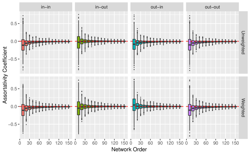
Figure 1: Boxplots of four kinds of weighted and unweighted assortativity coefficients for 2,000 weighted and directed ER random networks; the red dashed line in each panel is $\rho=0$.

Figure 1 shows the boxplots of the assortativity coefficients for the 2,000 networks against the network order $n$. For comparison, we also included the four kinds of directed but unweighted assortativity coefficients (Foster et al., 2010). All the assortativity coefficients converge to $0$ quickly. For a moderate network order $n=150$, all the assortativity coefficients are centered around $0$ with small variation. There is no significant difference between any pair of weighted and unweighted assortativity measures. No obvious difference in convergence rate is observed, either. Since the extended ER random networks are completely random networks, where the edges are added independently, the fact of no tendency of vertex connection is well reflected by the assortativity coefficients.

3.2 Barabási–Albert Random Networks

The Barabási–Albert (BA) random network model (Barabási and Albert, 1999) defines a generative network with a preferential attachment mechanism. Starting from a seed graph, at each evolutionary step, a new vetex is connected with an existing vertex with probability proportional to its degree. BA networks are scale-free networks because their degree sequence obeys a power law (Bollobás et al., 2001). van der Hofstad and Litvak (2014) showed that the assortativity of an undirected and unweighted BA network is asymptotically $0$. The assortativity of weighted and directed BA networks has not been investigated before.

Our construction of weighted and directed BA networks is extended from the algorithm of Wan et al. (2017). The seed graph consists of two vertices connected by a directed edge. The edge addition process is controlled by tow parameters $\alpha,\gamma\in[0,1]$ subject to $\alpha+\gamma=1$. With probability $\alpha$, an edge is added from a newcomer to a sampled vertex in the existing network; with probability $\gamma$, an edge is added from a sampled vertex in the existing network pointing in the newcomer. The weight of each edge is drawn independently from a pre-specified distribution with positive support. The probability of an existing vertex being sampled at each step is proportional to its in-strength or out-strength, instead of its in-degree or out-degree as in Wan et al. (2017); the choice between in-strength and out-strength depends on the direction of the newly added edge. Additional tuning parameters $\delta_{\rm out}$ and $\delta_{\rm in}$ control the growth rate of out-strength and in-strength, respectively.

We set $\alpha=0.6$, $\gamma=0.4$, and $\delta_{\rm in}=\delta_{\rm out}=1$, and drew edge weight from a discrete uniform distribution over $\{1,2,\ldots,10\}$. To investigate the relation between network order and assortativity, we considered network order $n\in\{2^{4},2^{5},\ldots,2^{12}\}$. For each setting, 2,000 independent networks were generated. Figure 2 shows the boxplots of weighted and unweighted out-in assortativity coefficients; the plots for out-out, in-in, and in-out assortativity coefficients are similar and, hence, omitted. Both weighted and unweighted assortativity coefficients are negative, with the weighted version closer to zero. The negative assortativity is expected since new vertices (of out- or in-strength $1$) tend to be connected with the vertices of large out-strength or in-strength vertices in the existing network. When network size becomes larger, both assortativity values get closer to zero with small variations.

Figure 2: Side-by-side boxplots of weighted and unweighted out-in assortativity coefficients for 2,000 BA random networks of different size.

Edge weight may have significant impact on network assortativity. To illustrate, we considered adding an edge with a substantially large weight as network grows. Under the same setting of $\alpha,\gamma,\delta_{\rm in}$ and $\delta_{\rm out}$, we generated BA networks with $500$ steps (i.e., equivalently $502$ vertices). There is one edge with weight $1,000$, while all of the others have relatively small weights, drawn uniformly from $\{1,2,\ldots,10\}$. The arrival time of the large-weight edge was set at $t\in\left\{10,20,\ldots,500\right\}$. For each $t$, a total of 2,000 networks were generated, and the weighted and unweighted out-in assortativity coefficients were calculated.

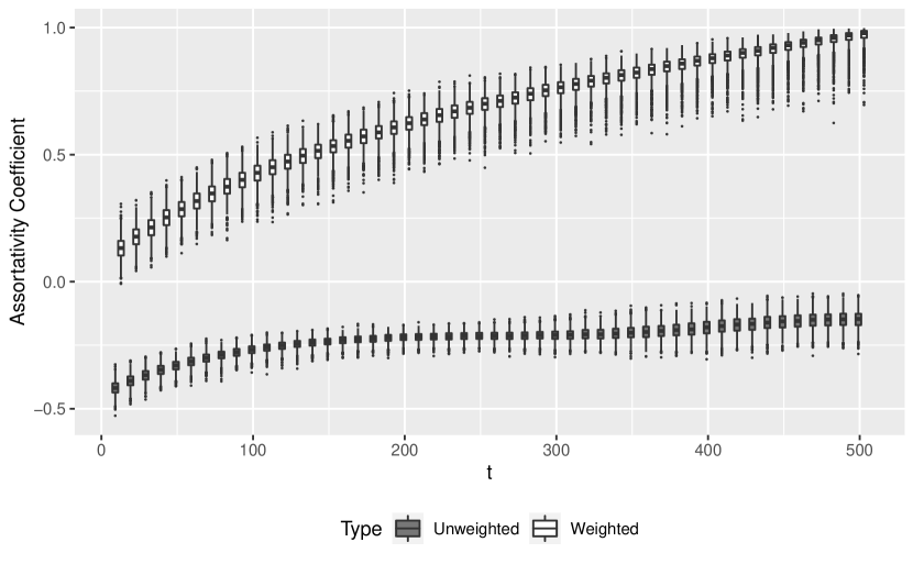
Figure 3: Side-by-side boxplots of weighted and unweighted out-in assortativity coefficients of BA random networks (fixed size 500), with one large-weight edge joining in at different timestamps.

Figure 3 shows the boxplots of the weighted and unweighted out-in assortativity coefficients against the arrivale time of the big-weight edge. Unlike in Figure 2, here the weighted and unweighted assortativity coefficients appear to be drastically different. The weighted assortativity coefficients are positive, but the unweighted counterparts stay negative. The later the large-weight edge joins the network, the higher the weighted out-in assortativity coefficient is. Especially when the large-weight edge is the last one, it ensures that the edge links a vertex of large out-strength to a vertex of large in-strength. Since the weights of all preceding edges are relatively small, the contributions to the weighted out-in assortativity is dominated by the last large-weight edge, and thus the assortativity reaches a high value. When the large-weight edge is appended to the network at an early time, the vertices at the two ends at its first appearance have high probabilities to attract the subsequent newcomers; the weighted assortativity coefficient remains positive owing to the impact of the large weight, but its effect is tapered off over time. The unweighted assortativity coefficients remain negative and show no response to arrival time of the big-weight edge, which does not reflect the expected changes.

3.3 Stochastic Block Models

The stochastic block model (SBM, Holland et al., 1983) is a class of network models presenting community structures. The vertices in a network based on SBM are partitioned into disjoint communities such that the number of edges among the vertices within a community is expected to be significantly higher than that among the vertices from different communities. One of the classical edge addition algorithms for generating an SBM is a two-step procedure. Within each community, generate an ER random graph with a relatively large value of $p$; between communities, generate an edge with probability $p^{\prime}<p$ between each pair of between-community vertices. The set of $p$ and $p^{\prime}$ may vary from community to community.

We considered SBM networks consisting of two communities of equal size. The link density for each community was fixed at $p=0.2$, and the edge weights within each community were sampled uniformly from $(0,5)$ and $(5,10)$, respectively. The between-community link density was set to be $p^{\prime}=0.02$, independent of within-community edges. The between-community edge weights were set to be identically $5$. The edge directions were assigned randomly with equal probability and independently, for both within- and between-community edges. We allowed the community size to vary in $\{50,100,\ldots,500\}$. For each setting, we generated 2,000 SBM networks and calculated their weighted and unweighted out-in assortativity coefficients.

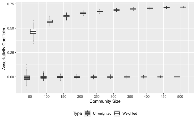
Figure 4: Side-by-side boxplots of weighted and unweighted out-in assortativity coefficients based on 2,000 SMB networks with different community sizes.

Figure 4 shows the side-by-side boxplots of the weighted and unweighted out-in assortativity coefficients against the community size. The unweighted assortativity coefficients are centered around $0$ with small variations regardless of the change in community size (and network size). That is expected as the edges are added independently, and the edge weights are ignored in the computations of unweighted assortativity coefficients. Each of the simulated networks is structurally equivalent to a composition of two (mutually independent) ER random graphs and an independent Bernoulli model, leading to $0$ assortativity. When the edge weights are accounted, however, the assortativity coefficients are obviously positive with higher values for the networks of larger size. The within-community edges always link the vertices with large out-strength to those with large in-strength (or the vertices with small out-strength to those with small in-strength). The between-community link density is relatively small, and the between-community edges are likely to link two isolated vertices when the communities are large in size. Thus, the weighted out-in assortativity coefficients tend to be positive, especially for large networks.

To investigate the impact of between-community edge weight and link density on network assortativity, we conducted a a sensitivity analysis. The changes to the settings are: the community size was fixed at $500$; the between-community link density parameter was set to be $p^{\prime}\in\{0.02,0.03,\dots,0.1\}$; and the between-community edge weights were set to be identically $5k$ with $k\in\{1,1/2,1/4,1/8\}$. For each configuration, $2,000$ SBMs were generated. The boxplots of the weighted out-in assortativity coefficients are summarized in Figure 5. As expected, the assortativity coefficient decreases as $p^{\prime}$ increases for each given $k$; the decreasing is faster for smaller $k$. For each given $p^{\prime}$, the assortativity coefficient increases as $k$ decreases, and the increase is faster for higher $p^{\prime}$. The results support that both between-community edge weight and link density have impact on assortativity values.

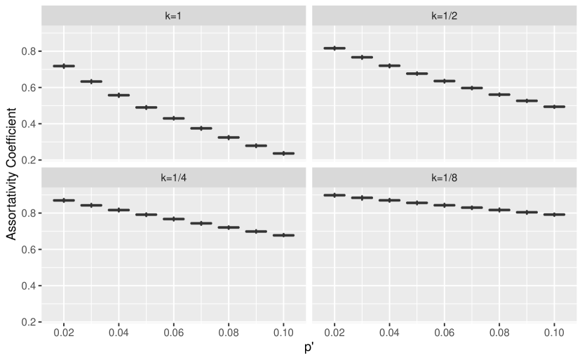
Figure 5: Weighted out-in assortativity coefficients of SMB networks by choosing different values of ratio $k$ and $p^{\prime}$.

3.4 Rewired Networks with Given Assortativity

A weighted (undirected) network can be rewired so that its assortativity achieves a predetermined level by extending the algorithm of Newman (2003). The details of our rewiring algorithm are given in Appendix D. Let $\xi$ be the target assortativity coefficient of a weighted network of $n$ vertices. Let $S$ denote a random variable of admissible vertex strength with support $\mathcal{S}$, where $|\mathcal{S}|<\infty$. We generated networks with $n=2,000$ vertices whose strengths are distributed such that $p_{k}=\Pr(S=z_{k})\propto z_{k}^{-2.5}\exp{-z_{k}/100}$ for $z_{k}\in\mathcal{S}=\left\{10,11,\dots,99,100\right\}$. The number of rewiring steps was fixed at $5000\times n$. For each $\xi\in\left\{0.1,0.2,0.3,\dots,0.8,0.9\right\}$, 100 networks were simulated.

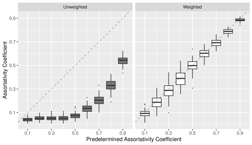
Figure 6: Boxplots of the weighted and unweighted assortativity coefficients of the simulated networks with respect to different predetermined values.

Figure 6 shows the boxplots of both weighted and unweighted assortativity coefficients of the 100 simulated networks against $\xi$. The weighted assortativity coefficients (right panel) are approximately centered on the $45$-degree line, suggesting that the average of the weighted assortativity coefficients are consistent with the predetermined values. The boxplots of the unweighted assortativity coefficients (left panel), however, stay far away from the $45$-degree line, implying that the unweighted assortativity coefficient fails to capture the assortative feature of the weighted network.

4 Application to WIONs

We apply the proposed measures to WIONs constructed with the 2016 release of the World Input-Output database (Timmer et al., 2015). There have been a few studies of the WIONs (Cerina et al., 2015; del Río-Chanona et al., 2017; Piccardi et al., 2017) with data based on the 2013 release. The 2016 release is the most recent, covering the period of 2001–2014. For each year, the WIOT records the directed economic transactions among 56 sectors of 44 countries, regions, or territories, the last one of which is the rest of the world (RoW). Therefore, the resulting WIONs have order 2,464. The edge weights are in the unit of million US dollars (USD). For the purpose of temporal comparison, an adjustment for inflation has been applied to the data using the GDP deflators from the World Bank (https://data.worldbank.org/indicator/NY.GDP.DEFL.ZS). The WIONs are extremely dense (e.g., the link density of the WION of 2014 is $0.83$), but contain a large amount of edges with small weights (e.g., the $90$-th percentile of the edge weights in the WION of 2014 is $0.81$ millions USD). The large amount of edges with small weights tend to blur the fundamental structure of the network that are of primary interest. One way to extract the fundamental structure is to use the backbone of the WION after discarding noisy edges up to a certain level. We adopt the filtering procedure introduced by Xu and Liang (2019); see details in Appendix E.

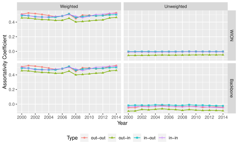
Figure 7: Weighted and unweighted assortativity coefficients of WIONs and their corresponding backbones at level $0.05$ from 2000 to 2014.

Figure 7 presents the four kinds of weighted assortativity coefficients from the whole WIONs and their backbones of level $0.05$ from 2000 to 2014. For comparison, with unweighted assortativity coefficients (Barrat et al., 2004) that were used by Cerina et al. (2015) are also included. In the upper-left panel, all four weighted assortativity measures for the whole WIONs are positive in the range from $0.40$ to $0.53$, suggesting that the vertices of similar strength levels are more likely to be connected. For instance, high-instrength region-sectors like “construction” usually take large inputs from high-outstrength region-sectors like manufactures of “mineral products”, “basic metals” and “wood and cork”. Another example is given by “manufactures of computer, electronic and optical products” supplying large outputs to some relevant region-sectors such as “computer programming, consultancy and related activities”. WIONs have revealed a geographical feature that large amount of monetary transactions usually occur among the region-sectors in the same country, while fewer or substantially smaller transactions are observed among the region-sectors across different countries. This geographical feature helps explain the positive values of the weighted assortativity measures for WIONs. The temporal changes in all assortativity coefficients appear to be quite similar. Each curve presents a notable from 2007 to 2008 when the global financial crisis occurred. After 2009, a consistently upward trend emerges in each curve, suggesting recovery of the global economy. The counterparts for the backbones show almost the same magnitude and patterns. The backbones of level 0.05 had only about 5% of the edges preserved but account for over 96% of the total weights. This shows the robustness of the proposed assortativity coefficients in capturing the fundamental structure of WIONs. In contrast, the unweighted assortativity coefficients are negative (close to $0$ in magnitude) with little temporal changes over the years, similar to those reported by Cerina et al. (2015). The dramatic difference between the weighted and unweighted results suggests that ignoring link weights in any kind of assortativity measure may lead to misleading conclusions.

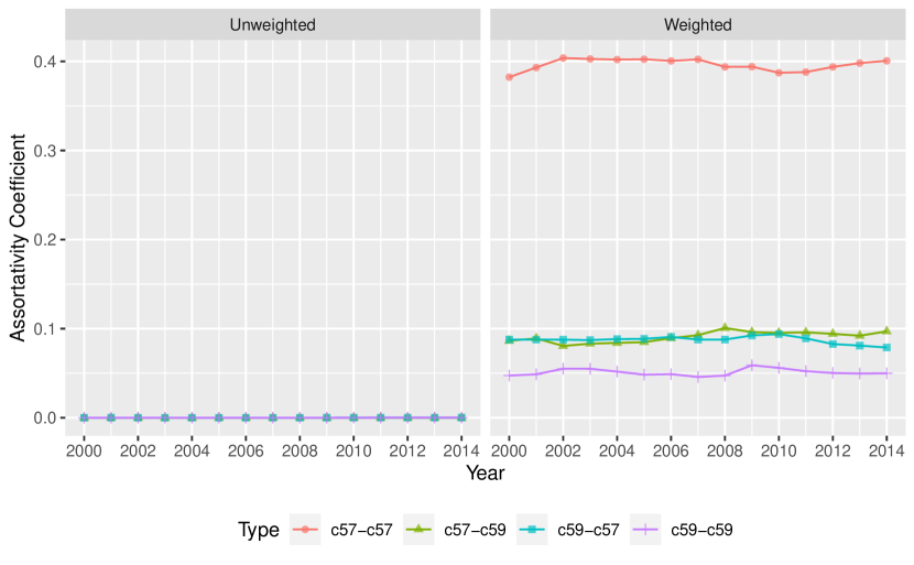
Figure 8: Assortativity coefficients between the final consumption expenditure by households ($c57$ denoted by $X$) and by government service ($c59$ denoted by $Y$) of WIONs from 2000 to 2014.

The WIONs provide a good opportunity to illustrate the applicability of the proposed assortativity measures to general vertex-specific features beyond degree and strength. Consider two vertex features, the final consumption expenditure by households ($c57$ denoted by $X$) and by government service ($c59$ denoted by $Y$). These features are in the WIOTs but not used in constructing the WIONs. Let $\rho_{\alpha,\beta}$, $\alpha,\beta\in\{X,Y\}$, be the assortativity coefficient between feature $\alpha$ of the source vertex and feature $\beta$ of the target vertex. Figure 8 shows the four assortativity coefficients (of both weighted and unweighted versions) for the periods of 2001–2014. All the weighted assortativity coefficients are positive. The level of $\rho_{X,X}$ is about 0.4, notably higher than the rest (0.1 or lower). This implies that the region-sectors with higher final consumption by households are likely transact more among themselves. The curve of $\rho_{X,X}$ fluctuates within a relatively small region over the 15 years. It has a noticeable increasing trend during 2000–2002, followed by stable period before a downward trend during 2008–2010, and rises steadily afterwards. The other three coefficients are closer to zero, suggesting no strong tendency of assortative connections. Of interest is that $\rho_{X,Y}$ and $\rho_{Y,X}$ stay together at about the same level over all the years, despite that they measure transactions of opposite directions. If edge weight is not accounted when analyzing the correlation of the features independent of network structure, all kinds of the assortativity measures are centered at $0$ with small variations (see the left panel in Figure 8), and hence become non-informative and useless.

5 Discussions

The proposed class of assortativity measures meet the practical need from analyses of weighted and directed network. Special cases of the proposed measures are equivalent to several classical assortativity measures in the literature. The generalized measures can be used to study the assortative tendency of any pair of vertex-specific features. Extensive simulations and two real data analyses demonstrate that both edge direction and weight should be accounted in the computation. Edge direction is an essential property, as a directed network may simultaneously present assortative and disassortative mixing, i.e., one kind of assortativity coefficient (e.g., out-in) may have a positive value, while another (e.g., in-out) has a negative value; see Piraveenan et al. (2012) for an example of food webs in the United States. Edge weight characterizes weighted networks; discarded it leads to meaningless results or incorrect conclusions.

The proposed assortativity measures, like Newman’s original measure, are still based on the concept of Pearson correlation coefficient. Newman’s measure converges to $0$ when network size is sufficiently large (Litvak and van der Hofstad, 2013), a drawback shared by the proposed measures. In addition, our simulation examples in Section 3.2 suggest that the proposed measures may not successfully characterize the assortativity of a network if the edge weights all have similar levels. One possible remedy is to extend assortativity measure based on Spearman’s correlation (Litvak and van der Hofstad, 2013). Along the same line, a few other nonparametric correlation coefficients in statistics can similarly be considered, such as Kendall’s tau and Blomqvist’s beta. We will continue our research in this direction, and report our outcomes elsewhere in the future.

Appendix A An Illustrative Example

For example, let us consider a weighted and directed network as shown in Figure 9. The weights are marked next to the directed edges; for example, $w_{AB}=10$, $s^{(\rm in)}_{A}=3$, $s^{(\rm out)}_{A}=13$, $s^{(\rm in)}_{B}=16$ and $s^{(\rm out)}_{B}=9$. Additionally, we have $\bar{s}_{\rm sou}^{\left(\rm out\right)}=9.39$, $\bar{s}_{\rm sou}^{\left(\rm in\right)}=5.90$, $\bar{s}_{\rm tar}^{\left(\rm out\right)}=5.90$, $\bar{s}_{\rm tar}^{\left(\rm in\right)}=10.16$, $\sigma_{\rm sou}^{\left(\rm out\right)}=3.68$, $\sigma_{\rm sou}^{\left(\rm in\right)}=6.58$, $\sigma_{\rm tar}^{\left(\rm out\right)}=4.83$, and $\sigma_{\rm tar}^{\left(\rm in\right)}=6.06$. For the given network, we have the weighted assortativity coefficients $\rho_{\rm in,in}=-0.56$, $\rho_{\rm in,out}=-0.82$, $\rho_{\rm out,in}=0.29$ and $\rho_{\rm out,out}=-0.29$. This example network simultaneously presents assorative and disassortative mixing. However, when edge weights are not accounted in the computation, the corresponding four kinds of assortativity coefficients are all equal to $-0.75$, suggesting strong disassortative mixing.

Figure 9: An illustrative example of weighted directed network.

Appendix B Variants of the Proposed Assortativity

Proposition 1.

The proposed assortativity coefficient is equivalent to that given by Arcagni et al. (2019) (case 4) when a network is weighted but undirected.

Proof.

For weighted but undirected networks, each weighted edge can be evenly split to two weighted and directed edges respectively pointing into the two vertices at the ends. In what follows, the strength of a node $i$, $s_{i}$, is equal to the sum of the manually created in-strength $\tilde{s}^{(\rm in)}_{i}$ and out-strength $\tilde{s}^{(\rm out)}_{i}$, i.e., $\tilde{s}^{(\rm in)}_{i}=\tilde{s}^{(\rm out)}_{i}=s_{i}/2$. The new arrangement causes a change in the weighted adjacency matrix; namely $\tilde{\bm{W}}=\bm{W}/2$ and consequently $\tilde{W}=\sum_{i,j\in V}\tilde{w}_{ij}=W/2$. As network direction is not accounted, the four kinds of assortativity measures are equivalent. Without loss of generality, we continue the verification by considering the “out-out” type. Elementary algebra leads us to

$$\bar{s}^{\,\rm(out)}_{\rm sou}=\bar{s}^{\,\rm(out)}_{\rm tar}=\frac{\sum_{i,j\in V}(w_{ij}/2)(s_{i}/2)}{W/2}=\frac{\sum_{i,j\in V}w_{ij}s_{i}}{2W}=\frac{\mu}{2},$$

where $\mu$ is the weighted average of $s_{i}$. The standard deviation is given by

$$\sigma^{\rm(out)}_{\rm sou}=\sigma^{\rm(out)}_{\rm tar}=\sqrt{\frac{\sum_{i,j}(w_{ij}/2)(s_{i}/2-\mu/2)^{2}}{W/2}}=\frac{1}{2}\cdot\sqrt{\frac{\sum_{i,j\in V}w_{ij}(s_{i}-\mu)^{2}}{W}}=\frac{\sigma}{2},$$

where $\sigma$ is the weighted standard deviation. In what follows, Equation (2) is reduced to

$$\rho=\frac{\sum_{i,j\in V}(w_{ij}/2)\bigl{[}(s_{i}/2-\mu/2)(s_{j}/2-\mu/2)\bigr{]}}{(W/2)(\sigma/2)(\sigma/2)}=\frac{\sum_{i,j\in V}w_{ij}\bigl{[}(s_{i}-\mu)(s_{j}-\mu)\bigr{]}}{W\sigma^{2}}$$

, which completes the proof. ∎

When a network $G$ is directed but unweighted, its adjacency matrix $\bm{W}=\bm{A}$ is dichotomous, and the strength, in-strength and out-strength of a vertex is equal to its degree, in-degree and out-degree, respectively. Thus, Equation (2) is reduced to

$$\rho_{\alpha,\beta}(G)=\frac{\sum_{i,j\in V}a_{ij}\left[\left(d_{i}^{(\alpha)}-\bar{d}_{\rm sou}^{\,(\alpha)}\right)\left(d_{j}^{(\beta)}-\bar{d}_{\rm tar}^{\,(\beta)}\right)\right]}{A\sigma_{\rm sou}^{(\alpha)}\sigma_{\rm tar}^{(\beta)}},$$ (3)

where $A:=\sum_{i,j\in V}a_{ij}=|E|$ counts the number of edges, and the statistics $\bar{d}_{\rm sou}^{\,(\alpha)}$, $\bar{d}_{\rm tar}^{\,(\alpha)}$, $\sigma_{\rm sou}^{(\alpha)}$ and $\sigma_{\rm tar}^{(\beta)}$ are defined analogously. This is equivalent to Foster et al. (2010, Equation (1)). In addition, Equation (3) is identical to Newman (2003, Equation (25)) for $(\alpha,\beta)=(\rm in,out)$, and respectively identical to Piraveenan et al. (2012, Equation (21)) and Piraveenan et al. (2012, Equation (22)) for $(\alpha,\beta)=(\rm out,out)$ and $(\alpha,\beta)=(\rm in,in)$ by using the notations therein.

When a network $G$ is unweighted and undirected, we further simplify Equation (2) to

$$\rho=\frac{\sum_{i,j\in V}a_{ij}\bigl{[}(d_{i}-\mu)(d_{j}-\mu)\bigr{]}}{A\sigma^{2}},$$

where $\mu=\sum_{i,j\in V}a_{ij}d_{i}/A$ and $\sigma=\sqrt{\sum_{i,j\in V}a_{ij}(d_{i}-\mu)^{2}/(4A)}$. Elementary algebra shows that the above expression is mathematically equivalent to Newman (2002, Equation (4)).

Appendix C Boundary Values of the Proposed Assortativity

Consider a network $G$ consisting of $n\geq 3$ vertices with weighted adjacency matrix given by

$$\begin{pmatrix}0&u_{1}&0&0&\cdots&0\\ 0&0&u_{2}&0&\cdots&0\\ u_{3}&0&0&0&\cdots&0\\ \vdots&\vdots&\vdots&\vdots&\ddots&\vdots\\ 0&0&0&0&\cdots&0\end{pmatrix},$$

for some $u_{1},u_{2},u_{3}>0$. Elementary algebra shows that $\rho_{{\rm in,out}}(G)=\rho_{{\rm out,in}}(G)=1$, suggesting that high out-strength vertices are all connected with high in-strength ones.

Consider $G^{\ast}$ structurally similar to $G$ but with a different weighted adjacency matrix given by

$$\begin{pmatrix}0&u_{1}&0&0&\cdots&0\\ u_{2}&0&u_{3}&0&\cdots&0\\ 0&0&0&0&\cdots&0\\ \vdots&\vdots&\vdots&\vdots&\ddots&\vdots\\ 0&0&0&0&\cdots&0\end{pmatrix}.$$

If $u_{1}$ is significantly smaller than $u_{2}$ and $u_{3}$ (like $u_{1}=o(\min\{u_{2},u_{3}\})$ or $u_{1}\to 0$), we have $\rho_{\rm out,out}(G^{\ast})\to-1$. For $u_{3}=0$ and $u_{1}\neq u_{2}$, we have $\rho_{\rm out,out}(G^{\ast})=-1$.

Appendix D Rewiring Algorithm

Given the vertex strength distribution, i.e., $p_{k}=\Pr(S=z_{k})$, $k=1,\ldots,|\mathcal{S}|$, for $z_{k}\in\mathcal{S}$, if, in addition, we assume that the probability of an edge being sampled is proportional to its weight, then the conditional probability of corresponding contribution added to the strength of the vertex at either end of that edge is given by $q_{k}=z_{k}p_{k}/\sum_{z_{h}\in\mathcal{S}}z_{h}p_{h}$. The algorithm of Newman (2003) requires a transition matrix $\bm{M}:=(m_{ij})$ of dimension $(|\mathcal{S}|\times|\mathcal{S}|)$ such that all the row sums and column sums are equal to $0$ with $\sum_{z_{j},z_{k}\in\mathcal{S}}z_{j}z_{k}m_{jk}=1$. The functionality of $\bm{M}$ is to bridge $q_{k}$ with a strength-based joint distribution for links. Specifically, let $\ell_{jk}$ be the probability that a vertex with strength $z_{j}$ and a vertex with strength $z_{k}$ is connected. We have

$$\ell_{jk}=q_{j}q_{k}+\xi\sigma_{q}^{2}m_{jk},$$ (4)

where $\sigma_{q}^{2}$ is the empirical variance of distribution $q$. The collection of $\ell_{jk}$ forms a strength-based distribution of edge connection, so $\ell_{jk}$ is required to fall in $[0,1]$ for all $j,k\in V$. Under the current setting, fundamental algebra can show that $\sum_{jk}l_{jk}=1$ for $l_{jk}$ defined in Equation (4).

Note that all the constraints for $m_{jk}$’s from $\bm{M}$ are linear. Though there may be more than one qualified $\bm{M}$ in practice, we shall choose an “optimal” $\bm{M}$ according to some sort of criterion such as matrix norm. In what follows, the construction of $\bm{M}$ has become a quadratic programming problem, which can be done through standard statistical programming software. Specifically, we used the quadprog package (Turlach et al., 2019) for R.

Now, we are ready to give the extended rewiring algorithm. The inputs for our algorithm are the pre-specified vertex strength distribution $p_{k}$ and the true assortativity $\xi$.

1. Sample $n$ strength values for the $n$ vertices from the strength distribution $p_{k}$, $k=1,\ldots,|\mathcal{S}|$.

2. Generate a random network on the $n$ vertices as described above.

3. Randomly select a pair of edges respectively denoted by $(v_{a},v_{b})$ and $(v_{c},v_{d})$, where $v_{a}$ and $v_{b}$, $v_{c}$ and $v_{d}$ are the vertices at the two ends of the selected edges. Correspondingly, let $s_{a}$, $s_{b}$, $s_{c}$ and $s_{d}$ be the strengths of those vertices. At each rewiring step, the probability that one unit weight is added to $(v_{a},v_{c})$ and $(v_{b},v_{d})$, and simultaneously one unit weight is taken away from $(v_{a},v_{b})$ and $(v_{c},v_{d})$ is given by

   $$\begin{cases}\displaystyle\frac{\ell_{s_{a}s_{c}}\ell_{s_{b}s_{d}}}{\ell_{s_{a}s_{b}}\ell_{s_{c}s_{d}}},\qquad&\mbox{if }\ell_{s_{a}s_{c}}\ell_{s_{b}s_{d}}<\ell_{s_{a}s_{b}}\ell_{s_{c}s_{d}};\\ 1,\qquad&\mbox{otherwise}.\end{cases}$$

   Note that, if $(v_{a},v_{c})$ or $(v_{b},v_{d})$ does not exist, and rewiring is executed, an edge (or two edges) is created; Similarly, if $(v_{a},v_{b})$ or $(v_{c},v_{d})$ is a unit-weight edge, and rewiring is executed, the edge (or both edges) is removed.

4. Repeat the rewiring procedure (in step 3) for a preset number of times, and return the resultant network. It is worth mentioning that the rewiring number needs to be sufficiently large in general, where the present study follows the guidance given by Bertotti and Modanese (2019).

Appendix E Backbone Extraction

The basic goal of backbone extraction is to filter out the non-essential edges. Xu and Liang (2019) applied a disparity filter method (Serrano et al., 2009) to extract backbones from input-output networks. Consider the null hypothesis that the normalized weights corresponding to the outgoing or incoming edges of a vertex are the spacings formed by uniformly distributed variables over the unit interval. Let $\tilde{w}^{(\rm out)}_{ij}=w_{ij}/s^{(\rm out)}_{i}$ and $\tilde{w}^{(\rm in)}_{ji}=w_{ji}/s^{(\rm in)}_{i}$ be the normalized out- and in-strength of vertex $i$, respectively. The number of outgoing and incoming edges of $i$ are its out-degree $d^{\,(\rm out)}_{i}$ and in-degree $d^{\,(\rm in)}_{i}$, respectively. Given that there are $d>1$ out- or in-edges for a vertex, under the null hypothesis, a normalized weight has density

$$p(x;d)=(d-1)(1-x)^{d-2},\quad 0<x<1,\quad d>1.$$

The p-values of edge $i$ with normalized out-strength $d^{\,(\rm out)}_{i}$ and in-strength $d^{\,(\rm in)}_{i}$ are, respectively,

$$\alpha_{ij}^{\,\rm(out)}=\int_{\tilde{w}^{(\rm out)}_{ij}}^{1}p(x;d^{\,(\rm out)}_{i})\differential x\quad\mbox{ and }\quad\alpha_{ij}^{\,\rm(in)}=\int_{\tilde{w}^{(\rm in)}_{ij}}^{1}p(x;d^{\,(\rm in)}_{i})\differential x.$$

Borrowing the idea of hypothesis testing, we preserve edge $e_{ij}$ if $\alpha_{ij}^{\,\rm(out)}<\alpha$ or $\alpha_{ij}^{\,\rm(in)}<\alpha$ as the null assumption of uniform assignment is rejected; otherwise, $e_{ij}$ is filtered out. In other words, an edge is preserved if the criterion is satisfied for at least one of the two vertices at the ends. For the very rare cases where $d^{\,(\rm out)}_{i}=d^{\,(\rm in)}_{j}=1$, some special treatments based on additional criteria are needed, as removing these edges may break the connectivity of the network, but these edges themselves do not actually contribute heterogeneity to the network. These rare cases do not occur in the WIONs, so the standard filtering procedure suffices.

References

- Abbate et al. (2018) Abbate, A., De Benedictis, L., Fagiolo, G., and Tajoli, L. (2018), “Distance-Varying Assortativity and Clustering of the International Trade Network,” Network Science, 6, 517–544.
- Abe and Suzuki (2006) Abe, S. and Suzuki, N. (2006), “Complex Earthquake Networks: Hierarchical Organization and Assortative Mixing,” Physical Review E, 74, 026113.
- Arcagni et al. (2017) Arcagni, A., Grassi, R., Stefani, S., and Torriero, A. (2017), “Higher Order Assortativity in Complex Networks,” European Journal of Operational Research, 262, 708–719.
- Arcagni et al. (2019) — (2019), “Extending Assortativity: An application to weighted social networks,” Journal of Business Research, in press, https://doi.org/10.1016/j.jbusres.2019.10.008.
- Barabási and Albert (1999) Barabási, A.-L. and Albert, R. (1999), “Emergence of Scaling in Random Networks,” Science, 286, 509–512.
- Barrat et al. (2004) Barrat, A., Barthélemy, M., Pastor-Satorras, R., and Vespignani, A. (2004), “The Architecture of Complex Weighted Networks,” Proceedings of the National Academy of Sciences of the United States of America, 101, 3747–3752.
- Bertotti and Modanese (2019) Bertotti, M. L. and Modanese, G. (2019), “The Configuration Model for Barabasi-Albert Networks,” Applied Network Science, 4, 32.
- Bollobás et al. (2001) Bollobás, B., Riordan, O., Spencer, J., and Tusnády, G. (2001), “The Degree Sequence of a Scale-Free Random Graph Process,” Random Structures & Algorithms, 18, 279–290.
- Catanzaro et al. (2004) Catanzaro, M., Caldarelli, G., and Pietronero, L. (2004), “Assortative Model for Social Networks,” Physical Review E, 70, 037101.
- Cerina et al. (2015) Cerina, F., Zhu, Z., Chessa, A., and Riccaboni, M. (2015), “World Input-Output Network,” PLOS One, 10, e0134025.
- del Río-Chanona et al. (2017) del Río-Chanona, R. M., Grujić, J., and Jensen, H. J. (2017), “Trends of the World Iput and Output Network of Global Trade,” PLOS One, 12, e0170817.
- Dorogovtsev et al. (2010) Dorogovtsev, S. N., Ferreira, A. L., Goltsev, A. V., and Mendes, J. F. F. (2010), “Zero Pearson Coefficient for Strongly Correlated Growing Trees,” Physical Review E, 81, 031135.
- Erdös and Rényi (1959) Erdös, P. and Rényi, A. (1959), “On Random Graphs I,” Publicationes Mathematicae Debrecen, 6, 290–297.
- Foster et al. (2010) Foster, J. G., Foster, D. V., Grassberger, P., and Paczuski, M. (2010), “Edge Direction and the Structure of Networks,” Proceedings of the National Academy of Sciences of the United States of America, 107, 10815–10820.
- Gilbert (1959) Gilbert, E. N. (1959), “Random Graphs,” Annals of Mathematical Statistics, 30, 1141–1144.
- Holland et al. (1983) Holland, P. W., Laskey, K. B., and Leinhardt, S. (1983), “Stochastic Blockmodels: First Steps,” Social Networks, 5, 109–137.
- Leung and Chau (2007) Leung, C. C. and Chau, H. F. (2007), “Weighted Assortative and Disassortative Networks Model,” Physica A: Statistical Mechanics and its Applications, 378, 591–602.
- Litvak and van der Hofstad (2013) Litvak, N. and van der Hofstad, R. (2013), “Uncovering Disassortativity in Large Scale-Free Networks,” Physical Review E, 87, 022801.
- McPherson et al. (2001) McPherson, M., Smith-Lovin, L., and Cook, J. M. (2001), “Birds of a Feather: Homophily in Social Networks,” Annual Review of Sociology, 27, 415–444.
- Newman (2002) Newman, M. E. J. (2002), “Assortative Mixing in Networks,” Physical Review Letters, 89, 208701.
- Newman (2003) — (2003), “Mixing Patterns in Networks,” Physical Review E, 67, 026126.
- Newman (2010) — (2010), Networks: An Introduction, New York, NY: Oxford University Press.
- Piccardi et al. (2017) Piccardi, C., Riccaboni, M., Tajoli, L., and Zhu, Z. (2017), “Random walks on the World Input-Output Network,” Journal of Complex Networks, 6, 187–205.
- Piraveenan et al. (2012) Piraveenan, M., Prokopenko, M., and Zomaya, A. (2012), “Assortative Mixing in Directed Biological Networks,” IEEE/ACM Transactions on Computational Biology and Bioinformatics, 9, 66–78.
- Piraveenan et al. (2008) Piraveenan, M., Prokopenko, M., and Zomaya, A. Y. (2008), “Local Assortativeness in Scale-Free Networks,” Europhysics Letters, 84, 28002.
- Raschke et al. (2010) Raschke, M., Schläpfer, M., and Nibali, R. (2010), “Measuring Degree-Degree Association in Networks,” Physical Review E, 82, 037102.
- Serrano et al. (2009) Serrano, M. Á., Boguñá, M., and Vespignani, A. (2009), “Extracting the Multiscale Backbone of Complex Weighted Networks,” Proceedings of the National Academy of Sciences of the United States of America, 106, 6483–6488.
- Timmer et al. (2015) Timmer, M. P., Dietzenbacher, E., Los, B., Stehrer, R., and de Vries, G. J. (2015), “An Illustrated User Guide to the World Input-Output Database: The Case of Global Automotive Production,” Review of International Economics, 23, 575–605.
- Turlach et al. (2019) Turlach, B. A., Weingessel, A., and Moler, C. (2019), quadprog: Functions to Solve Quadratic Programming Problems, R package version 1.5–8, https://CRAN.R-project.org/package=quadprog.
- van der Hofstad and Litvak (2014) van der Hofstad, R. and Litvak, N. (2014), “Degree-Degree Dependencies in Random Graphs with Heavy-Tailed Degrees,” Internet Mathematics, 10, 287–334.
- van Mieghem et al. (2010) van Mieghem, P., Wang, H., Ge, X., Tang, S., and Kuipers, F. A. (2010), “Influence of Assortativity and Degree-Preserving Rewiring on the Spectra of Networks,” The European Physical Journal B, 76, 643–652.
- Wan et al. (2017) Wan, P., Wang, T., Davis, R. A., and Resnick, S. I. (2017), “Fitting the Linear Preferential Attachment Model,” Electronic Journal of Statistics, 11, 3738–3780.
- Xu and Liang (2019) Xu, M. and Liang, S. (2019), “Input-Output Networks Offer New Insights of Economic Structure,” Physica A: Statistical Mechanics and Its Applications, 527, 121178.