Abstract

Scientifically evaluating soccer players represents a challenging Machine Learning problem. Unfortunately, most existing answers have very opaque algorithm training procedures; relevant data are scarcely accessible and almost impossible to generate. In this paper, we will introduce a two-part solution: an open-source Player Tracking model and a new approach to evaluate these players based solely on Deep Reinforcement Learning, without human data training nor guidance. Our tracking model was trained in a supervised fashion on datasets we will also release, and our Evaluation Model relies only on simulations of virtual soccer games. Combining those two architectures allows one to evaluate Soccer Players directly from a live camera without large datasets constraints. We term our new approach Expected Discounted Goal (EDG), as it represents the number of goals a team can score or concede from a particular state. This approach leads to more meaningful results than the existing ones that are based on real-world data, and could easily be extended to other sports.

Figure 1: Evolution of our Tracking and EDG model over time. The EDG model learns to capture actions with potential in a very general manner, and computes such potential with the player coordinates our Tracking model gathers from the live camera.

Figure 2: (a) The ET model computes the position of each entity. It then passes the coordinates to the online tracker to: (1): Compute the embedding of each player, (2): Warp each coordinate with the homography from HE. (b) The HE starts by doing a direct estimation of the homography. Available keypoints are then predicted and used to compute another estimation of the homography. Both predictions are used to remove potential outliers. (c) The REID model computes an embedding for each detected player. It also compares the IoU’s of each pair of players and applies a Kalman Filter to each trajectory.

1 Introduction

In the 1980s, at the Hong Kong Jockey Club, Bill Benter gathered data to create a statistical prediction model for horse-racing, which made him one of the most profitable gamblers of all time Chellel (2018). Data became essential in most sports, impacting all aspects of their ecosystem: performance, strategy, and transfers. Advanced Sports Analytics started in the United States; franchises in Baseball, American Football, and Basketball being the first to consider data as a key for improvement and success. In charge of scouting in Baseball minor leagues for Oakland Athletics in the 1990s, Billy Beane proved that it was possible to create a cost-efficient team by finding undervalued players Lewis (2003). Using sabermetrics to value players, his 2006 Athletics team ranked 5th best of the regular season while being 24th of 30 major league teams in player salaries. Most of the popular European sports are now beginning to follow the trend, and data departments hold a more and more significant position in major clubs. Ten years after Beane’s success story, in 2016 and 2017, Liverpool FC respectively acquired Sadio Mané for £34 million and Mohamed Salah for £39 million thanks to a significant push from their director of research Ian Graham, Cambridge Ph.D. Schoenfeld (2019). These two key players led Liverpool FC to a historical 2019 Champions League victory in Madrid. Today, Sadio Mane’s and Mohamed Salah’s contracts are worth more than £100 million each.

One way of finding such an undervalued soccer player is to find alternative metrics to the traditional ones such as number of goals or passes accuracy. Here, we will present a general framework for soccer player evaluation from live camera: a tracking model processing camera’s input into players’ coordinates, and an Expected Discounted Goal (EDG) model evaluating an action based on each player tracking data. The particularity of our approach comes from the idea that our EDG model is trained purely on simulation, and never on real soccer data. This makes it much easier to train, and utterly independent from large soccer datasets that are either too complicated to produce, or too expensive to acquire.

Our EDG model generalizes well to many playstyles and many teams. It also produces similar or even more accurate results than existing models.

Our tracking model predicts the player’s coordinates and computes precise results even on difficult scenes such as sunny or covered with shadow ones. This is also the first end-to-end open-source framework for soccer player tracking, and could easily be extended to other team sports.

2 Related Work

2.1 Tracking players on a sport field

Player detection. Detecting soccer players can be a complicated task, especially in a multi-actors situation. There are multiple ways of doing this detection, Kaarthick (2019) explored the usage of a HOG color based detector that gives each image a detection of the players. Johnson (2020) worked on a deeper model: an open-source multiperson pose estimator named AlphaPose, based on the COCO dataset. Another approach is to consider players as objects and use Object Detection Models. Ramanathan et al. (2015) used such a model, a CNN-based multibox detector for the player detection.

Field registration. One key element of any sports tracking model is how players coordinates can be represented in two dimensions. One way to do so is Sport Field Registration, the act of finding the homography placing a camera view into a two-dimensional view, fixed across the entire game. More about Field Registration can be found in the Supplementary Materials-A. Sharma et al. (2017) formulated the registration problem as a nearest neighbor search over a generated dictionary of edge maps and homography pairs that they made synthetically. To extract the edge data from their images, they compared 3 different approaches: Histogram of oriented gradients (HOG) features, chamfer matching, and convolution neural networks (CNN). Finally, they enhanced their findings using Markov Random Field (MRF). Homayounfar et al. (2017) figured out the homography’s attributes by parametrizing the problem as one of inference in an MRV which features they determine using structured SVMs. The use of synthetic data is also explored by Chen & Little (2018), which takes Homayounfar et al. (2017) and Sharma et al. (2017)’s work one step further by building a generative adversarial network (GAN) model. Finally, Jiang et al. (2019) used a ResNet to directly predict the homography parameters iteratively, while Citraro et al. (2020) used particular keypoints detected with a Unet from the field to achieve the same goal.

Entities tracking in Video.

Ramanathan et al. (2015) used a Kanade–Lucas–Tomasi feature tracker for player tracking across a game. Recent ReIdentification models go a step further: Zheng et al. (2019) used an embedding model to extract player features, and a mixture of IoU and embedding similarities to track persons. Another approach was used by Liang (2020), with a k-Shortest Path algorithm and an embedding model to extract players’ numbers and colors.

2.2 Valuing player actions

Before the revolution brought by data analysis in football, valuing players was mostly based on traditional statistics such as the number of goals, the number of assists, passes accuracy, or the number of steals. These post-game statistics can be relevant as an overview of a player’s quality, but it does not reflect how a player can impact a game thanks to his vision or his moves. Furthermore, focusing on general statistics also means ignoring the entire universe of actions in which a player took part. Thanks to the growing availability of event and tracking data, researchers started to create models using all game events and tracking data to evaluate players’ actions on and off-ball. In 2018, Spearman (2018) suggested an indicator to evaluate off-ball positioning called Off-Ball Scoring Opportunities (OBSO). Thanks to his previous fundamental works on Pitch Control (PC), he was able to measure the positioning quality of attacking players by evaluating the danger of their position if they would receive the ball.

The same year, using tracking data, Fernández & Bornn (2018) presented two main indicators to measure the use of space and its creation during a game: Space Occupation Gain (SOG), and Space Generation Gain (SGG). Later on, in 2019, Fernández (2019) adapted Expected Possession Value (EPV), a deep learning based method, from basketball to football enabling analysts to reach a goal probability estimator at each instant of a possession. By discounting EPV, researchers were able to access the impact of a single event like a key pass which would increase significantly EPV. Similarly, Decroos et al. (2019) presented their VAEP model for which they developed an entire language around event data called Soccer Player Action Description Language (SPADL). Thanks to supervised learning, their model was trained to evaluate the impact an event could have on the scoring or conceding probability. Therefore, this model enables analysts to estimate the effect of each action from a player and then evaluate his global performance.

We start by going into the Theoretical framework of both our tracking model and our EDG model. In Experimental methods, we review the implementations and learning procedures of our models. Finally, in Results, we quickly present the tracking results to focus more on the insights given by our EDG model.

3 Theoretical framework

3.1 Tracking model

Our EDG model needs to know the state of the game at any time $t$: we chose to do so by representing a Soccer game with a list of entities coordinates. Given a list of images, our tracking model computes the 2-dimensional trajectories of both the ball and each player. The model adopts a 3-steps method: Entity Tracking, Homography Estimation, ReIdentification (see Figure 2) (ET,HE,REID). Each of these steps is represented by one or several models, and more theoretical background on the homography estimation can be found in the Supplementary Materials-A. The first 2 steps do not consider any temporal information as they approximate results for each image separately. However, the last step compares each new image to the list of images that have already been processed. Doing so allows us to take into consideration each entity’s movement over time and counters the mistakes the previous models might do. We quickly review here each of the 3 steps: ET, HE, REID.

Entity Tracking definition. The ET : $\mathbb{R}^{n\times n\times 3}\to\mathbb{R}^{m\times 4}\times\left[0,1\right]^{m}\times\left[0,1\right]^{m}$, takes an image as input, and predicts a list of bounding boxes associated with a class prediction (Player or Ball) and a confidence value.

Homography Estimation definition. The HE is made of 2 separate models. The first one : $\mathbb{R}^{n\times n\times 3}\to\mathbb{R}^{3\times 3}$ takes an image as input, and predicts the homography directly. The second one : $\mathbb{R}^{n\times n\times 3}\to\mathbb{R}^{p\times n\times n}$ also takes an image as input, but predicts $p$ masks, each mask representing a particular keypoint on the field (see Figure 3). The homography is computed knowing the coordinates of available keypoints on the image, by mapping them to the keypoints coordinates on a 2-dimensional field (see Supplementary Materials-A for more details). Using both models allows us to have better result stability, and to use one model or the other when outliers are detected.

ReIdentification definition. The REID model gathers all information from the ET model and builds the embedding model as well. The embedding model : $\mathbb{R}^{n\times n\times 3}\to\mathbb{R}^{751}$ takes the image of a detected player, and gives a meaningful embedding. The model initializes several tracklets based on the boxes from ET in the first image. In the following ones, the model links the boxes to the existing tracklets according to: (1): their distance measured by the embedding model, (2): their distance measured by boxes IoU’s. A Kalman Filter Kalman (1960) is also applied to predict the location of the tracklets in the current image and removes the ones that are too far from the linked detection. The model also updates the embedding of each player over time with another Kalman Filter.

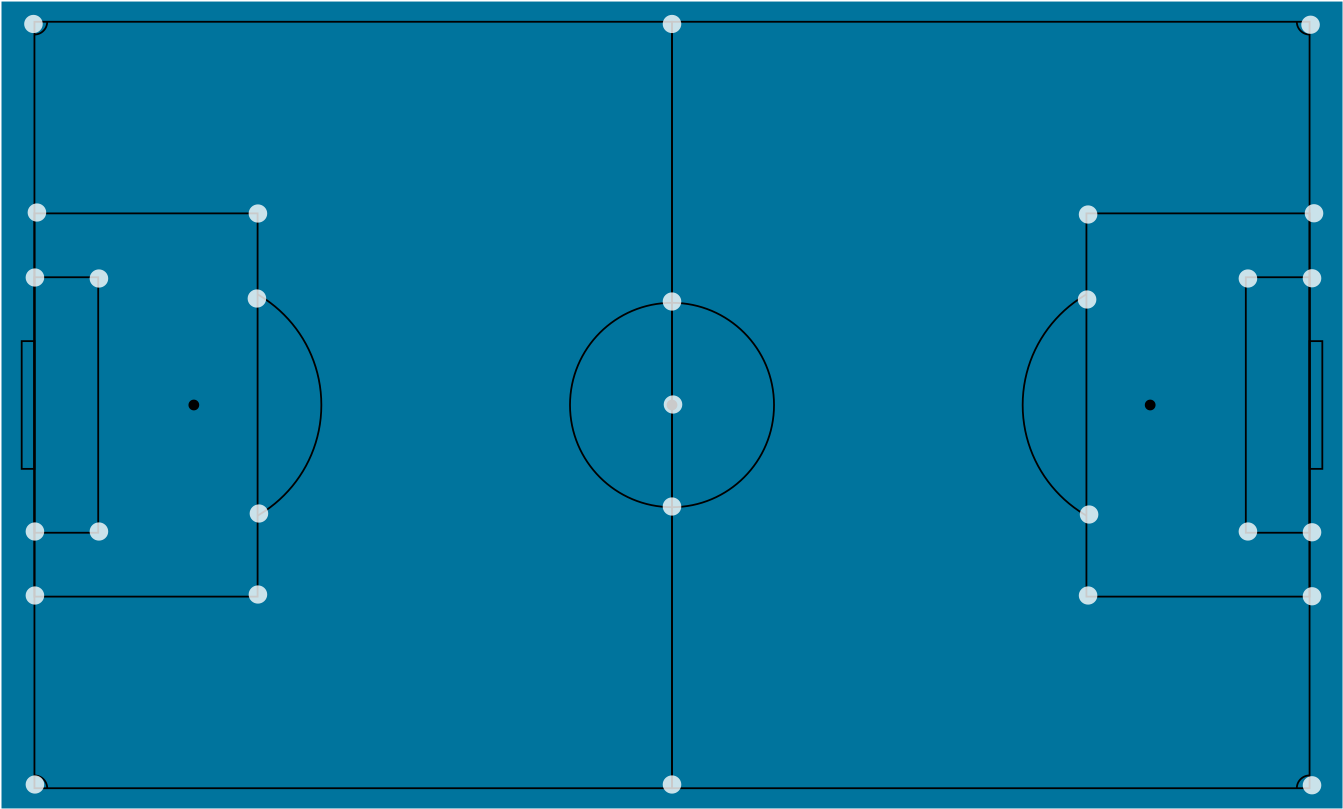
Figure 3: Positions of the $28$ keypoints the HE model predicts. During training and inference, each keypoint is associated with a different mask. Such a mask is a binary matrix, with $1$s at the position of the keypoint, and $0$s elsewhere. We have $28$ masks, one per keypoint.

3.2 EDG model

We assume $s_{t}\in\mathcal{S}$ is the state of the game at time $t$. It may be the positions of each player and the ball for example. Given an action $a\in\mathcal{A}$ (e.g.a pass, a shot, more details in the Supplementary Materials-B), and a state $s^{\prime}\in\mathcal{S}$, we note $\mathbb{P}\colon\mathcal{S}\times\mathcal{A}\times\mathcal{S}\to[0,1]$ the probability $\mathbb{P}(s^{\prime}|s,a)$ of getting to state $s^{\prime}$ from $s$ following action $a$. Applying actions over $K$ time steps yields a trajectory of states and actions, $\tau^{t_{0:K}}=\big{(}s_{t_{0}},a_{t_{0}},...,s_{t_{K}},a_{t_{K}}\big{)}$. We denote $r_{t}$ the reward given going from $s_{t}$ to $s_{t+1}$ (e.g.$+1$ if the team scores a goal). More importantly, the cumulative discounted reward along $\tau^{t_{0:K}}$ is defined as:

$$R(\tau^{t_{0:K}})=\sum_{n=0}^{K}\gamma^{n}r_{t_{n}}$$

where $\gamma\in\left[0,1\right]$ is a discount factor, smoothing the impact of temporally distant rewards.

A policy, $\pi_{\theta}$, chooses the action at any given state, whose parameters, $\theta$, can be optimized for some training objectives (such as maximizing $R$). Here, a good policy would be a policy representing the team we want to analyze in the right manner. The Expected Discounted Goal (EDG), or more generally, the state value function, is defined as:

$$V^{\pi}(s)=\underset{\tau\sim\pi}{\mathbb{E}}\big{[}R(\tau)|s\big{]}$$

It represents the discounted expected number of goals the team will score (or concede) from a particular state. To build such a good policy, one can define an objective function based on the cumulative discounted reward:

$$J(\theta)=\underset{\tau\sim\pi_{\theta}}{\mathbb{E}}\big{[}R(\tau)\big{]}$$

and seek the optimal parametrization $\theta^{*}$ that maximize $J(\theta)$:

$$\theta^{*}=\arg\max_{\theta}\mathbb{E}\big{[}R(\tau)\big{]}$$

To that end, we can compute the gradient of such cost function $\nabla_{\theta}J(\theta)$ to update our parameters with $\theta\leftarrow\theta+\lambda\nabla_{\theta}J(\theta)$. In our case, the evaluation of $V^{\pi}$ and $\pi_{\theta}$ is done using Neural Networks, and $\theta$ represents the weights of such networks (more details on Neural Networks can be found in Goodfellow et al. (2017)). At inference, our model will take the state of the game as input, and will output the estimation of the EDG. A more advanced view of Reinforcement Learning can be found in Sutton & Barto (1998)

4 Experimental methods

All of the models were implemented using standard deep learning libraries and the usual image processing library. Models, code, and datasets will be released at https://github.com/DonsetPG/narya.

4.1 Tracking implementation details

Entity Tracking details. The ET model is based on a Single Shot MultiBox Detector (SSD) Liu et al. (2016). The model takes images of shape $(512,512)$, and makes prediction for 2 classes: players (including referees) and the ball. We used an implementation from GluonCV Guo et al. (2020).

Homography Estimation details. The first model (direct estimation) is based on a Resnet-18 architecture He et al. (2015). It takes images of shape $(280,280)$ and randomly crops images of shape $(256,256)$ during training. The model doesn’t directly estimate the homography, but rather the coordinates of 4 control points, in the same manner as Jiang et al. (2019). More details can be found in Supplementary Materials-A. The model is implemented with Keras Chollet et al. (2015). The second model is based on an EfficientNetb-3 backbone Tan & Le (2019) on top of a Feature Pyramid Networks (FPN) Lin et al. (2016) architecture to predict the mask of each keypoint. We implemented our model using Segmentation Models Yakubovskiy (2019).

ReIdentification details. The embedding model is based on a Resnet-50 architecture He et al. (2015) to produce embeddings of size $751$. The model was produced for supervised Re-Identification Zheng et al. (2019) and implemented on Torch Paszke et al. (2017).

4.2 DRL implementations details

The EDG model is based on a Deep Reinforcement Learning environment Kurach et al. (2019) built by the Google Brain Team and based on a gym environment Brockman et al. (2016).

States, actions, and reward representations. Each state $s$ is represented by a Super Mini Map (SMM), stacked 4 times to represent the last 4 positions of each entity. More precisely, $s\in\mathbb{R}^{72\times 96\times 16}$, where each consecutive 4 matrices encode the positions of the home team, the away team, the ball, and the active player (leading to $4\times 4=16$ for third dimension). The encoding is binary in $\{0,255\}$, representing whether an entity is at the given coordinates or not.

The actions $a$ include movements in 8 directions, different kicks (e.g.  short and long passes, shooting), and high passes. Each action is sticky, meaning that once executed, a moving or sprinting action will not stop until explicitly told to do so. The reward $r\in\{-1,0,1\}$ represents if a goal is conceded, not happening or scored.

EDG model details. The DRL agent, capturing the policy and the EDG is represented by a PPO Schulman et al. (2017) algorithm, with an Impala policy Espeholt et al. (2018). The architecture is available Figure-4.

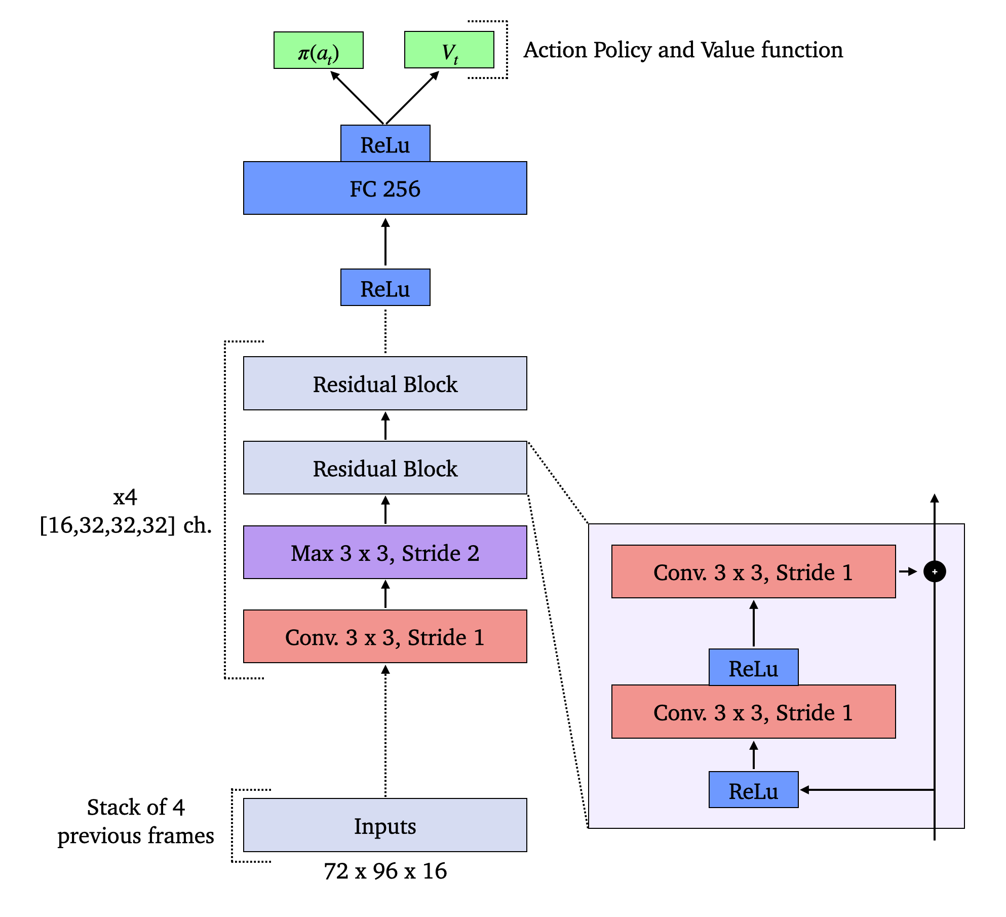
Figure 4: Architecture used for our agent.

4.3 Training

4.3.1 Tracking models

Datasets. We built 3 datasets: a tracking dataset, a homography dataset, and a keypoint dataset. They all consist of the same images from the 2014 World Cup, the Premier League, the Ligue 1, and the Liga. They typically contain $450$ train images, $50$ validation images, and $50$ test images. The homography dataset was based on an existing 2014 World Cup dataset Homayounfar et al. (2017). We extended it to the rest of our images. More details on the datasets can be found in the Supplementary Materials-B.

Data augmentation. The models were trained on a Tesla-P100 GPU, and each model takes a few hours to train. In each training we used data augmentation : (1): Use the entire original input image, (2): Randomly flip the image horizontally, (3): Randomly add Gaussian Noise and shadows on the field, (4): Randomly change the brightness, the contrast, and the saturation, (5): Add motion blur.

Optimization procedures. Both of the homography models were trained for $200$ epochs, with a batch size of $32$ and a learning rate of $10^{-4}$. We used an exponential learning rate decay down to $10^{-8}$. The tracking model was trained for $100$ epochs, with a batch size of $2$ and a learning rate of $10^{-3}$. The embedding model was pretrained on the Market-1501 dataset Zheng et al. (2015). Each model was evaluated each $5$ training epochs, and we stopped training when we observed a negligible decrease in the loss function. Each model was trained using an Adam optimizer Kingma & Ba (2014).

4.3.2 DRL Agent

Selfplay. We started with a pretrained Agent from Google, trained from 50M steps against an easy bot. We then kept training it for 50M steps against a medium bot. Finally, we trained the agent another 50M against the last version of itself twice. While previous results Kurach et al. (2019) were mitigated about self-play, we believe that given the significant advantage our agent had against a medium bot, it was the right decision to improve its capability to find actions with potentials. We compare the results of agents with and without selfplay Figure 7 (right) and in the Supplementary Materials-C.3.

Optimization procedures. The agent was trained on $8$ parallel environments with a learning rate of $.000343$ and a discount factor $\gamma$ of $0.993$. We use $8$ minibatches per epoch and update our agent $4$ times per epoch. Finally, the agent is updated with a batch size of $1024$, using an Adam optimizer again. More details on the hyperparameters can be found in the Supplementary Materials-C.2 Figure C.4.

4.4 Evaluation

The homography estimation models use the IoU between the warped field with our estimation and ground truth homography as the primary metric. We used the mean Average Precision (mAP) for the tracking model for bounding boxes with an IoU greater than $0.5$. Finally, we did not use any metric for the ReIdentification model, as the model we used was not finetuned on a Soccer player dataset. Mode details on the metrics, results, and hyperparameters can be found in the Supplementary Materials-C.

We report the result of our DRL agent both with the Average Goal Difference against its opponent and by comparing the EDG to existing frameworks on the same actions. This allows both to grasp the policy’s level and how close it reacts to policy based on real players.

5 Results

Our main findings are that the EDG model can have a relevant representation of the potential of an action. It can even detect events that previous frameworks could not, even though the agent never trained on real game data. Furthermore, the tracking model can produce reliable coordinates for short plays from only one camera. This model allows us to produce the EDG of any given action quickly. We start by quickly reviewing the results of our Tracking model in Section 5.1. In Section 5.2 and 5.3, we present the results of the EDG model and compare it to existing value frameworks.

We kept the same agent and the same tracking models throughout the results to challenge their robustness to different scenarios or teams.

5.1 Generating players’ coordinates

Figure 5: We can track almost every player and the ball, even in very different settings. We present here some examples of tracking failures and success. In sequence (a), the REID model fails to identify player 19 between frame 1. and 2., letting the same player having a new id (15). Between frames 3., 4. and 5., the boxes of players 4 and 5 merge into id 20. When the merge is undone, the model can retrieve the right id for each player
In sequence (b), the same phenomenon appears frame 2., 3. and 4. but the model fails to recognize player 8 and gives him a new id (16). Another issue with our model is when a player runs out of the camera’s range and returns later. This almost always leads to a change of id, as seen in frame 5. with player 17. However, this can easily be managed by merging the two ids trajectories.

We found that each component of the Tracking Model generalizes well to many scenarios. We start by reviewing the results for each component and leave discussion about some architectural choices to the Supplementary Materials.

Method	IoU - Mean	IoU - median
OURS	0.908	0.921
OURS, keypoints	0.892	0.923
OURS, direct estimation	0.891	0.906
Keypoints, with Playersa	0.939	0.955
Keypoints, w/o Playersa	0.905	0.918
Synthetic Dictionaryb	0.914	0.927
Learned Errorsc	0.898	0.929
Branch and Boundd	0.83	-
PoseNete	0.528	0.559
SIFTf	0.170	0.011

Table 1: Quantitative results of the Homography estimator models on the 2014 World Cup dataset. Even though Citraro et al. (2020) obtain better results with their method when using the positions of players as well, we believe that our results where good enough for our purpose, which was to provide reliable tracking data to our EDG model.
^a Citraro et al. (2020), ^b Sharma et al. (2017), ^c Jiang et al. (2019), ^d Homayounfar et al. (2017), ^e Kendall et al. (2015), ^f Lowe (2004)

Backbone	Player - AP	Ball - AP	mAP
VGG16	89.3	39.5	64.4
Resnet50	89.9	59.3	74.6

Table 2: Quantitative results of the player Tracking model, with a SSD model. More details about the results for less impactfull choices can be found in the Supplementary Materials-C

Architecture	Backbone	IoU	F1-Score
Unet	EfficientNetb-3	0.817	0.831
LinkNet	EfficientNetb-3	0.813	0.828
FPN	EfficientNetb-3	0.882	0.91
	Resnet18	0.862	0.885
	Resnet50	0.841	0.863

Table 3: Quantitative results for the keypoints masks generations. More details about the results for other backbones can be found Figure C.2

Entity Tracking results. The main results are available in Table 2. Overall, the Resnet50 backbone yields much better results than the VGG16. The Average Precision for the player class is about $90\%$, where the mistakes often come from stacks of players that are hard to distinguish even for the human eye. Because of its relatively small size and its frequent occlusion by players, the ball Average Precision does not get higher than $60\%$.

Homography Estimation results. The results and comparison against existing methods are available Table 1. We find similar results to Citraro et al. (2020) for our Keypoints based method and slightly better results than the direct estimation implementation from Jiang et al. (2019). This can be explained by the higher number of dense layers added at the end of our Resnet18 architecture. Our combination of 2 very different strategies allows the complete model to react better to outliers and bypass the condition of 4 non-collinear points needed by the keypoints based model. Producing high-quality estimations of the homography is a hard task with many consequences. If an estimation is incorrect, players’ coordinates will be as bad and produce noisy or false trajectories. For this reason, it is useful to manually check some estimations by hand during the tracking process, and remove them if they are too far from the truth. The more detailed results of the keypoints mask prediction are available in Table 3.

ReIdentification results. Since we have no dataset of soccer player re-Identification, it is impossible to evaluate our embedding model. However, we can denote the number of operations we had to do manually after a tracking is produced. On average, we had to delete $3.5$ trajectories per action (one trajectory to remove every $60.57$ frame, or $3$ seconds, on average). This number includes the referees that we also detect in our dataset and model. We merge $5$ trajectories per action on average (e.g.when a player is not recognized and gets a new id). Finally, we manually add $3.75$ missing coordinates on average, mostly when we do not find the ball at a critical moment (e.g.  the beginning of a pass or a shot).

We present the results of our entire model Figure 5 for $2$ different actions, and give a more in-depth analysis of when our model successfully tracks each player even when the tracking model fails to detect them, but also highlight particular cases of Re-Identification failure. We discuss in the Supplementary Materials-C the rest of architectural choices. We also display more results for each model in Figure C.3.

5.2 Valuing expected discounted goals

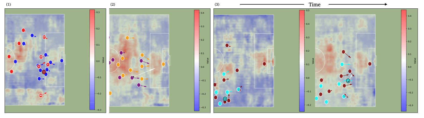
Figure 6: EDG mapping based on the position of the ball. In (1), passing the ball to the midfield would release pressure and increase the EDG, but lose momentum. A forward pass inside the box or to the right-wing would also increase the EDG and keep the current momentum. In (2), a forward pass to the right-wing would have less impact as one inside the box, given the current players’ velocities. We present in (3) an evolution of the EDG overtime. In the first frame, a pass to the middle would help release the high pressure. The team prefers to stay on the right side and to create a momentum towards the goal. The EDG evolves then to increase on the wing. The EDG does not take into account the different physical capabilities of each player, thus underestimate the potential the team attack’s speed.

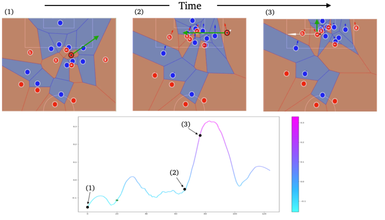
Figure 7: (left) We present here the EDG over time alongside the tracking of players. The green arrows represent the action taken in the next frame by the player. Between frame (1) and (2), the EDG increases with the long forward pass to the right-wing. It keeps increasing frame (2) to (3) with a decisive pass inside the box, before decreasing due to the very high pressure. It increases again with a shot.
(right) Comparison between our agent EDG map and an agent trained for 50M steps against an easy bot. The easy agent attribute on average the same potential to every location on the field. It shows how training against a more difficult agent and self-play helped our agent learn real soccer players’ behavior.

Our Agent imparts a satisfactory understanding of soccer and soccer dynamics, even while training on simulations. First, Table 4 shows the Average Goal Difference between our Agent and its opponent at the end of each training step ($50$M updates): not only does the Agent learn to beat easy and medium bots, but it also learns more complex dynamics while training against itself. The major impact of this selfplay component can be seen Figure 7 (right), and in the Supplementary Materials Figure C.4. We displayed on these maps the EDG estimated by our Agent if the ball was located at this location. After the first 2 steps of training, the Agent attributes on average the same EDG to each location of the field. After selfplay, a more realistic and insightful potential is discovered.

This potential can be seen Figure 6 for 4 different games. While the front of the center circle and penalty sport both get a high EDG (for releasing the pressure and a high probability of goal respectively), the Agent also accurately captures the most dangerous zones. For example, in both Figure 6 (1) and (2), a forward pass to the right-wing would bring a lot of value to the action. Since the Agent inputs take into consideration the four last frames, it can consider each entity’s velocity.

Our model can also estimate the EDG of an action over time. We present 7 (left) the evolution of the EDG during an action, with the player tracking as well. While our Agent can capture the potential of an action, we believe that 2 components make the EDG extremely valuable for soccer analysis:

The discount factor, $\gamma$. We chose a discount factor of $0.993$, meaning that if a goal takes place 100 frames later, it brings a value of $0.993^{100}\approx 0.5$. It reduces the bias from which a single goal would bring immense value to each previous action, even ones that are far away. This allows linking each action to the goal they might lead to realistically, without any arbitrary tricks. The value of a goal is, therefore, more uniformly distributed over actions.

The expected value, $\underset{\tau\sim\pi_{\theta}}{\mathbb{E}}$. First, the Expected Value allows the EDG to get closer to the concept of almost-goal, which means that we want to remove any randomness in soccer and consider equal a goal or a shot striking the goalposts for example. Equivalently, we don’t want to consider too many outliers, such as lucky goals. This has two effects: a better estimation of the real potential of an action, and better detection of undervalued (resp. overvalued) actions and players. Most importantly, it forces analysis to focus on what leads to a goal, not on the shot itself.

Training Step	Opponent	Average Goal Difference
Step 1	Easy Bot	8.14
Step 2	Medium Bot	4.7
Step 3	end of Step 2	5.3
Step 4	end of Step 3	4.8

Table 4: Average Goal Differences at the end of the training between our Agent and the opponent.

5.3 Comparison with existing framework

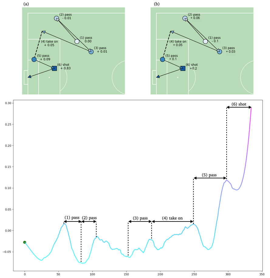
Figure 8: We compare here on the same scenario, VAEP Decroos et al. (2019) (a) and our EDG (b). Our EDG is negative on pass (1), as we take into account the 2 close surrounding opponents to the receiver. The next 2 passes are highly important, and get more values in our framework as they allow to: (2) release pressure, (3) add momentum and danger close to the goal. The next two actions get overall the same value as the VAEP. However, the shot gets a much smaller value within our framework, as our model discounts the goal and attributes more uniformly the potential of an action.

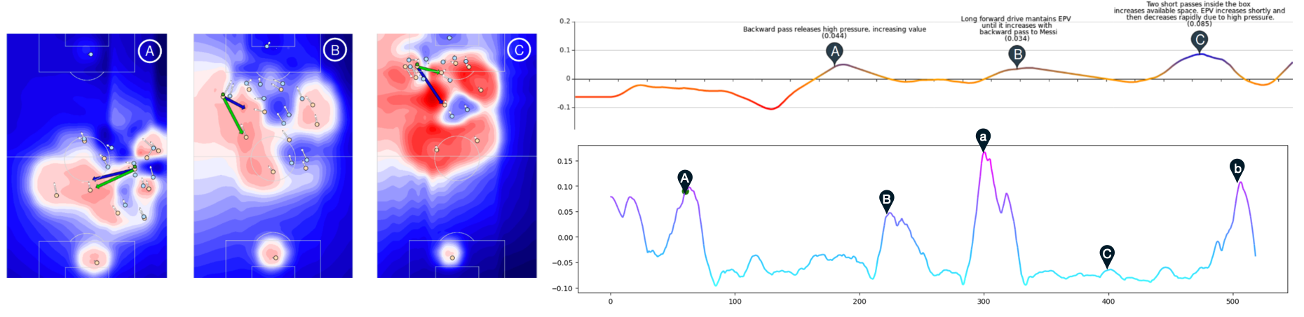
Figure 9: We compare here in the same scenario the EPV Fernández (2019) and our EDG. We pick up the same increase in value for action A and B, while our model doesn’t value as much action C. On the other hand, our model values a lot action a, which is a long forward pass to the left-wing, and a strong situation that could lead crossing the ball to a teammate. We also kept track of the end of the action (situation b) with a great pass followed by a caught header.

One way to ensure our Agent produces good analysis is to compare it to other algorithms whose purpose is to evaluate soccer players. We focus on 2 different models: the Expected Possession Value (EPV) from Fernández (2019), and Valuing Actions by Estimating Probabilities (VAEP) from Decroos et al. (2019). We compare the three approaches to the scenario they used on their paper, as we do not have access to their training procedures or their data.

Overall, we find that our approach, while never trained on data extracted from a real game, find on average the same value as the other 2 approaches. The EPV and our Agent always agree on the positive or negative impact of an action, and when the surrounding is not too impactful, the VAEP and our Agent also agree on the value of an action.

It does, however, find more precise and meaningful values for more subtle actions. This is a powerful result and proof that our Agent learnt realistic soccer behaviors in a simulation, and can understand and process information at various levels: e.g.action a player can perform, pressing on a player, players’ velocities. For example, a forward pass would get a good value from the VAEP algorithm, while our Agent could give him a weak value because opponents are close, or if a pass is risky because of the field limits. Overall, we find that the value of a goal is much more uniformly distributed in the previous actions with our framework. For example, an assist and its related goal would get values distribution of 10% and 90% in the other frameworks, while our Agent would give a distribution of 35% and 65%.

6 Conclusion

We presented a generic framework for soccer player tracking and evaluation based on machine learning and Deep Reinforcement Learning. Our experiments show that we can produce trajectories of players only from a single camera and that our EDG framework captures more insightful potential than previous models, while being based on simulations. We find that both the tracking model and EDG agent are the first open-sourced one while being more accurate than previous approaches.

Regarding the tracking models, our model could easily be extended to other sports, with appropriate datasets. Some improvements may be obtained by building a soccer ReIdentification datasets or building Unsupervised Approach.

Our DRL Agent would benefit a lot from being replaced by a multi-agent algorithm, where more than one player are being controlled at once. Improvements over the soccer environment would also help a lot: bringing more physical statistics for players or particular teams, for example. While we focus on pure simulation-based training, finetuning the Agent on Expert Data from real games could help to bridge the gap with a more realistic playstyle.

Finally, this work aims to give a broader audience access to soccer tracking data and analysis tools. We also hope that our datasets will help to build more performant models over time.

 

Supplementary Material: Evaluating Soccer Player: from Live Camera to Deep Reinforcement Learning

 

Appendix A Supplementary Homography model details

We assume 2 sets of points $(x_{1},y_{1})$ and $(x_{2},y_{2})$ both in $\mathbb{R}^{2}$, and define $\mathbf{X_{i}}$ as $[x_{i},y_{i},1]^{\top}$. We define the planar homography $\mathbf{H}$ that relates the transformation between the 2 planes generated by $\mathbf{X_{1}}$ and $\mathbf{X_{2}}$ as :

$$\mathbf{X_{2}}=\mathbf{H}\mathbf{X_{1}}=\begin{bmatrix}h_{11}&h_{12}&h_{13}\\ h_{21}&h_{22}&h_{23}\\ h_{31}&h_{32}&h_{33}\end{bmatrix}\mathbf{X_{1}}$$

where we assume $h_{33}=1$ to normalize $\mathbf{H}$ and since $\mathbf{H}$ only has $8$ degrees of freedom as it estimates only up to a scale factor. An example of such homography is available Figure A.1 (left). The equation above yields the following 2 equations:

$$x_{2}=\frac{h_{11}x_{1}+h_{12}y_{1}+h_{13}}{h_{31}x_{1}+h_{32}y_{1}+1}$$

$$y_{2}=\frac{h_{21}x_{1}+h_{22}y_{1}+h_{23}}{h_{31}x_{1}+h_{32}y_{1}+1}$$

that we can rewrite as :

$$x_{2}=h_{11}x_{1}+h_{12}y_{1}+h_{13}-h_{31}x_{1}x_{2}-h_{32}y_{1}x_{2}$$

$$y_{2}=h_{21}x_{1}+h_{22}y_{1}+h_{23}-h_{31}x_{1}y_{2}-h_{32}y_{1}y_{2}$$

or more concisely:

$$\begin{bmatrix}x_{1}&y_{1}&1&0&0&0&-x_{1}x_{2}&-y_{1}x_{2}\\ 0&0&0&x_{1}&y_{1}&1&-x_{1}y_{2}&-y_{1}y_{2}\end{bmatrix}\mathbf{h}=0$$

where $\mathbf{h}=[h_{11},h_{12},h_{13},h_{21},h_{22},h_{23},h_{31},h_{32}]^{\top}$. We can stack such constraints for $n$ pair of points, leading to a system of equations of the form $\mathbf{A}\mathbf{h}=0$ where $\mathbf{A}$ is a $2n\times 8$ matrix. Given the $8$ degrees of freedom and the system above, we need at least $8$ points (4 in each plan) to compute an estimation of our homography. This is the method we used to build the Homography Dataset, and is also the method we use to compute the homography after our keypoints predictions. An example of the points correspondences in Soccer is available Figure A.1 (right).

In reality, our Direct Estimation model doesn’t predict directly the $8$ homography parameters, but the coordinates of $4$ control points instead Jiang et al. (2019). The predicted coordinates of these $4$ control points are then used to estimate the homography using the system of equations above.

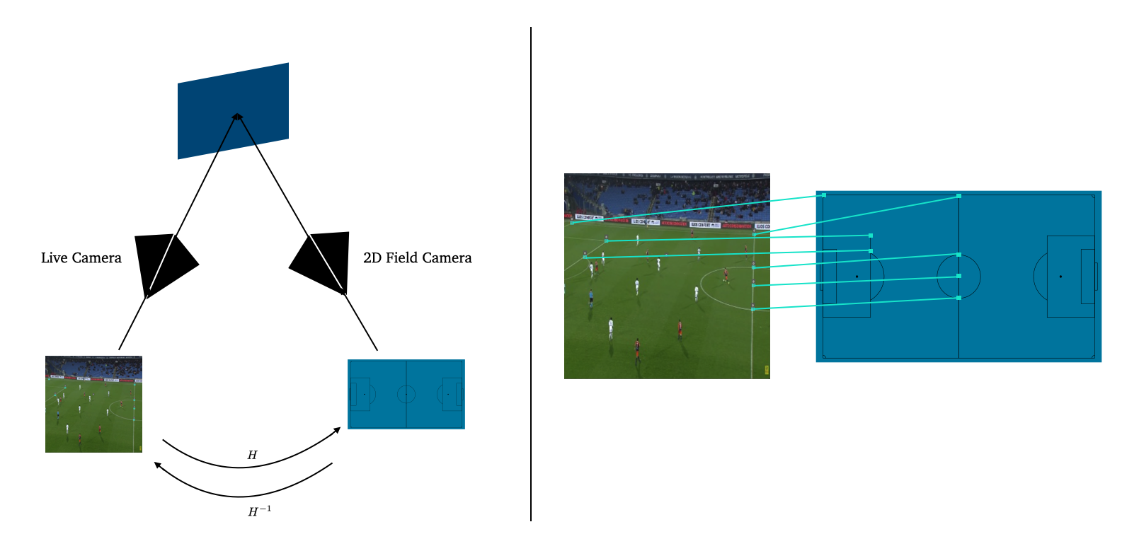
Figure A.1: (left) Example of a planar surface (our soccer field) viewed by two camera positions: the 2D field camera and the Live camera. Finding the homography between them allows to produce 2D coordinates for each player. (right) Example of points correspondences between the 2D Soccer Field Camera and the Live Camera.

Appendix B Supplementary datasets details

B.1 Overview

Name	Inputs	Outputs	# Train Images	# Validation Images	# Test Images	Examples
Tracking Dataset	$1024,1024$	Bounding Boxes	480	60	60	Figure B.1 (a)
Homography Dataset	$1280,720$	$3,3$	874	-	159	-
Keypoints Dataset	$320,320$	Keypoints	463	46	59	Figure B.1 (b)

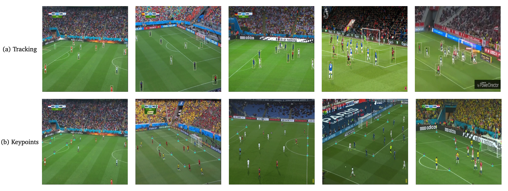
Figure B.1: Example of the Tracking Dataset (a), with the bounding boxes for Players, Referees and the Ball. In (b) are shown examples of the Keypoints Dataset, with the position of the keypoints highlighted in blue.

B.2 Actions for the DRL agent

The controlled player can move in 8 directions, sprinting or not. These actions are sticky, and will last until an action Stop Moving (resp. Stop Sprinting) is produced. They can also produce several sort of passes or shots, and interact with dribbles or slides. The full list of actions is available Table B.1.

Top	Bottom	Left	Right
Top Left	Top Right	Bottom Left	Bottom Right
Short Pass	High Pass	Long Pass	Shot
Do Nothing	Slide	Dribble	Stop Dribble
Sprint	Stop Moving	Stop Sprinting	-

Table B.1: List of actions the agent can chose at each timestep.

Appendix C Supplementary results

C.1 Architectural choices for tracking

In the following paragraph, we discuss some failed model experiments and architectural choices. Except for the entire model we presented above, we tested $4$ other different configurations:

1. Use a $2$-steps model for direct homography estimation,

2. Use a Multi-scale network for direct homography estimation,

3. Apply the tracking model to split images,

4. Smooth the homographies estimations over time,

For (1), we tried different scenarios based on a first direct homography estimation model. Giving the first model’s prediction to a second one, also based on Resnet18, does not improve the performance significantly ($0.8$%) (confirming previous results Jiang et al. (2019)). We also tried to stack the field warped with our homography estimation to our original image, but without any improvements at all. Finally, using both the warped field and the homography estimation doesn’t improve the performance either.

For (2), we implemented and trained a $3$-steps Multi-scale model from Le et al. (2020). This model progressively estimates and refines the homography from a third of the image to the entire one, in addition to the warped field from the previous step estimation. While promising, this model did not lead to better results. We believe that this is a result of the high degree of transformations there is between the field and the camera input. However, it can be a great model to estimate the homography modifications happening between $2$ consecutive frames.

For (3), we realized that producing the image in higher quality and then splitting it in separate panels allowed the tracking model to detect more players. An example is available Figure C.1. We compared the results of the tracking model on $3$ experiments: detection on the entire image (with shape ($1024,1024$), 4 detections on 4 panels (each of shape ($512,512$) and 8 detections on panels of shape ($256,256$). Overall, we found that the second experiment was leading to the best results.

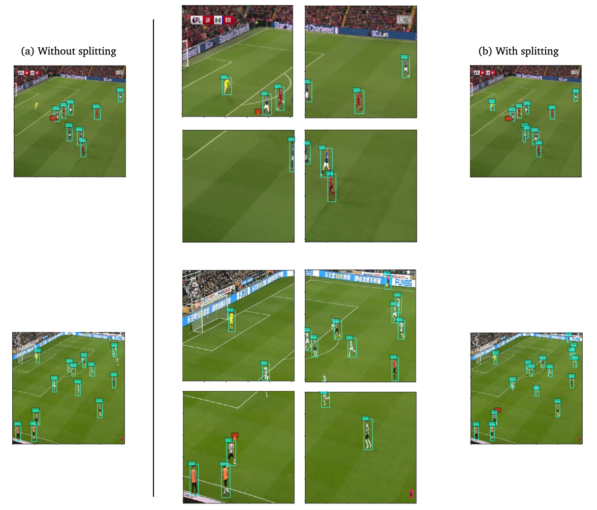
Figure C.1: Example of the difference in results between a direct prediction, and a splitted prediction. It gives better on results on average, while letting some players (the cropped ones) being missed. This issue can be addressed by using both the direct prediction and the splitted one.

For (4), we tried to apply a Sagvol filter to the sequence of estimated homographies over the entire action. However, the results were mitigated, as it would help the stability over time, but would completely ruin the tracking as soon as one outlier was produced. To avoid such behaviour, we ended up using no filter to the sequence of homographies.

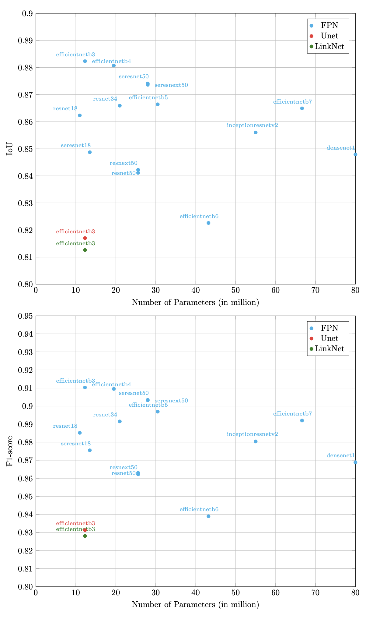
Figure C.2: Ablation study on the keypoints dataset to generate masks. Each model is plotted based on its number of parameters and its metric. We only tested one backbone for the LinkNet et Unet architecture because of the poor results in comparison to the FPN.

C.2 Expected Discounted Goal: hyperparameters

Parameter	Value
Clipping Range	0.08
Discount Factor	0.993
Entropy Coefficient	0.003
GAE	0.95
Gradient Norm Clipping	0.64
Learning Rate	.000343
Number of Actors	16
Training Epochs per Update	2
Value Function Coefficient	0.5

Table C.1: Hyperparameters used for each global step of the Agent training. We reused these for selfplay too.

C.3 Tracking and homography: supplementary results

See Figure C.3 for an overview of the results for each model on random images.

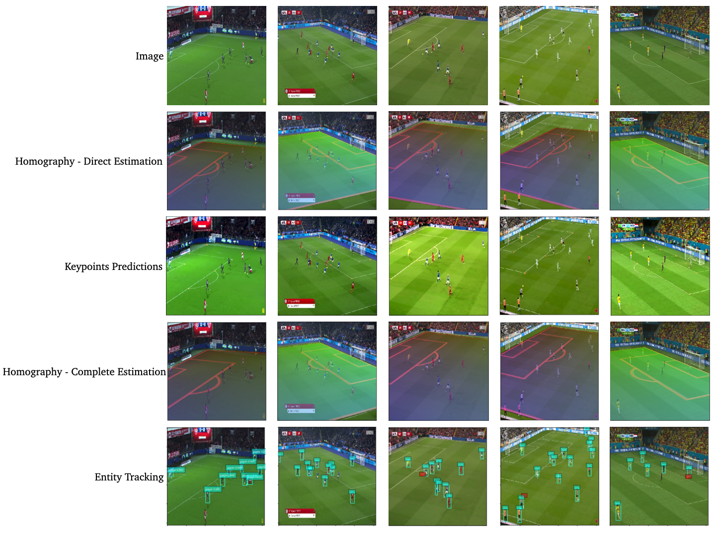
Figure C.3: Additional results from each model of our tracking model. Each image was selected randomly and not cherry picked.

C.4 Expected Discounted Goal: supplementary results

See Figure C.4 for another example of our agent versus an agent trained only against an easy bot.

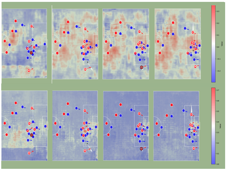
Figure C.4: Another example following the idea from Figure 7 (right). Again, we show here how the easy Agent doesn’t grasp any meaningful information from the game.

References

- Brockman et al. (2016) Brockman, G., Cheung, V., Pettersson, L., Schneider, J., Schulman, J., Tang, J., and Zaremba, W. Openai gym, 2016.
- Chellel (2018) Chellel, K. The gambler who cracked the horse-racing code. Bloomberg L.P., 05 2018.
- Chen & Little (2018) Chen, J. and Little, J. J. Sports camera calibration via synthetic data. CoRR, abs/1810.10658, 2018. URL http://arxiv.org/abs/1810.10658.
- Chollet et al. (2015) Chollet, F. et al. Keras. https://keras.io, 2015.
- Citraro et al. (2020) Citraro, L., Márquez-Neila, P., Savarè, S., Jayaram, V., Dubout, C., Renaut, F., Hasfura, A., Ben Shitrit, H., and Fua, P. Real-time camera pose estimation for sports fields. Machine Vision and Applications, 31(3), Mar 2020. ISSN 1432-1769. doi: 10.1007/s00138-020-01064-7. URL http://dx.doi.org/10.1007/s00138-020-01064-7.
- Decroos et al. (2019) Decroos, T., Bransen, L., Van Haaren, J., and Davis, J. Actions speak louder than goals. Proceedings of the 25th ACM SIGKDD International Conference on Knowledge Discovery and Data Mining - KDD, 2019. doi: 10.1145/3292500.3330758. URL http://dx.doi.org/10.1145/3292500.3330758.
- Espeholt et al. (2018) Espeholt, L., Soyer, H., Munos, R., Simonyan, K., Mnih, V., Ward, T., Doron, Y., Firoiu, V., Harley, T., Dunning, I., Legg, S., and Kavukcuoglu, K. Impala: Scalable distributed deep-rl with importance weighted actor-learner architectures, 2018.
- Fernández (2019) Fernández, J., B. L. . C. D. Decomposing the immeasurable sport: A deep learning expected possession value framework for soccer. 2019.
- Fernández & Bornn (2018) Fernández, J. and Bornn, L. Wide open spaces: A statistical technique for measuring space creation in professional soccer. 03 2018.
- Goodfellow et al. (2017) Goodfellow, I., Bengio, Y., and Courville, A. The Deep Learning Book. MIT Press, 2017.
- Guo et al. (2020) Guo, J., He, H., He, T., Lausen, L., Li, M., Lin, H., Shi, X., Wang, C., Xie, J., Zha, S., Zhang, A., Zhang, H., Zhang, Z., Zhang, Z., Zheng, S., and Zhu, Y. Gluoncv and gluonnlp: Deep learning in computer vision and natural language processing. Journal of Machine Learning Research, 21(23):1–7, 2020. URL http://jmlr.org/papers/v21/19-429.html.
- He et al. (2015) He, K., Zhang, X., Ren, S., and Sun, J. Deep residual learning for image recognition, 2015.
- Homayounfar et al. (2017) Homayounfar, N., Fidler, S., and Urtasun, R. Sports field localization via deep structured models. In 2017 IEEE Conference on Computer Vision and Pattern Recognition (CVPR), pp. 4012–4020, 2017.
- Jiang et al. (2019) Jiang, W., Higuera, J. C. G., Angles, B., Sun, W., Javan, M., and Yi, K. M. Optimizing through learned errors for accurate sports field registration, 2019.
- Johnson (2020) Johnson, N. Extracting player tracking data from video using non-stationary cameras and a combination of computer vision technique. 2020.
- Kaarthick (2019) Kaarthick, P. An automated player detection and tracking in basketball game. Computers, Materials & Continua, 58:625–639, 01 2019. doi: 10.32604/cmc.2019.05161.
- Kalman (1960) Kalman, R. E. A new approach to linear filtering and prediction problems” transaction of the asme journal of basic. 1960.
- Kendall et al. (2015) Kendall, A., Grimes, M., and Cipolla, R. Posenet: A convolutional network for real-time 6-dof camera relocalization, 2015.
- Kingma & Ba (2014) Kingma, D. P. and Ba, J. Adam: A method for stochastic optimization, 2014.
- Kurach et al. (2019) Kurach, K., Raichuk, A., Stanczyk, P., Zajac, M., Bachem, O., Espeholt, L., Riquelme, C., Vincent, D., Michalski, M., Bousquet, O., and Gelly, S. Google research football: A novel reinforcement learning environment, 2019.
- Le et al. (2020) Le, H., Liu, F., Zhang, S., and Agarwala, A. Deep homography estimation for dynamic scenes, 2020.
- Lewis (2003) Lewis, M. Moneyball: The Art of Winning an Unfair Game. 2003.
- Liang (2020) Liang, Q.; Wu, W. Y. Y. Z. R. P. Y. X. M. Multi-player tracking for multi-view sports videos with improved k-shortest path algorithm. Appl. Sci., 864, 2020.
- Lin et al. (2016) Lin, T.-Y., Dollár, P., Girshick, R., He, K., Hariharan, B., and Belongie, S. Feature pyramid networks for object detection, 2016.
- Liu et al. (2016) Liu, W., Anguelov, D., Erhan, D., Szegedy, C., Reed, S., Fu, C.-Y., and Berg, A. C. Ssd: Single shot multibox detector. Lecture Notes in Computer Science, pp. 21–37, 2016. ISSN 1611-3349. doi: 10.1007/978-3-319-46448-0˙2. URL http://dx.doi.org/10.1007/978-3-319-46448-0_2.
- Lowe (2004) Lowe, D. Distinctive image features from scale-invariant keypoints. International Journal of Computer Vision, 60:91–, 11 2004. doi: 10.1023/B:VISI.0000029664.99615.94.
- Paszke et al. (2017) Paszke, A., Gross, S., Chintala, S., Chanan, G., Yang, E., DeVito, Z., Lin, Z., Desmaison, A., Antiga, L., and Lerer, A. Automatic differentiation in pytorch. 2017.
- Ramanathan et al. (2015) Ramanathan, V., Huang, J., Abu-El-Haija, S., Gorban, A. N., Murphy, K., and Fei-Fei, L. Detecting events and key actors in multi-person videos. CoRR, abs/1511.02917, 2015. URL http://arxiv.org/abs/1511.02917.
- Schoenfeld (2019) Schoenfeld, B. How data (and some breathtaking soccer) brought liverpool to the cusp of glory. New York Times, 05 2019. URL https://www.nytimes.com/2019/05/22/magazine/soccer-data-liverpool.html.
- Schulman et al. (2017) Schulman, J., Wolski, F., Dhariwal, P., Radford, A., and Klimov, O. Proximal policy optimization algorithms, 2017.
- Sharma et al. (2017) Sharma, R. A., Bhat, B., Gandhi, V., and Jawahar, C. V. Automated top view registration of broadcast football videos. CoRR, abs/1703.01437, 2017. URL http://arxiv.org/abs/1703.01437.
- Spearman (2018) Spearman, W. Beyond expected goals. 03 2018.
- Sutton & Barto (1998) Sutton, R. S. and Barto, A. G. Introduction to Reinforcement Learning. MIT Press, Cambridge, MA, USA, 1st edition, 1998. ISBN 0262193981.
- Tan & Le (2019) Tan, M. and Le, Q. V. Efficientnet: Rethinking model scaling for convolutional neural networks, 2019.
- Yakubovskiy (2019) Yakubovskiy, P. Segmentation models. https://github.com/qubvel/segmentation_models, 2019.
- Zheng et al. (2015) Zheng, L., Shen, L., Tian, L., Wang, S., Wang, J., and Tian, Q. Scalable person re-identification: A benchmark. In Proceedings of the IEEE International Conference on Computer Vision, 2015.
- Zheng et al. (2019) Zheng, Z., Yang, X., Yu, Z., Zheng, L., Yang, Y., and Kautz, J. Joint discriminative and generative learning for person re-identification. IEEE Conference on Computer Vision and Pattern Recognition (CVPR), 2019.