A phenomenological estimate of the Covid-19 true scale
from primary data

Abstract

Estimation of the prevalence of undocumented SARS-CoV-2 infections is critical for understanding the overall impact of CoViD-19, and for implementing effective public policy intervention strategies. We discuss a simple yet effective approach to estimate the true number of people infected by SARS-CoV-2, using raw epidemiological data reported by official health institutions in the largest EU countries and the USA.

1 Introduction

As the coronavirus disease 2019 (CoViD-19) epidemic reached every corner of the world, each country has adopted different interventions to manage the early and long-term phases of the spread of the epidemic. This epidemic has forced many countries to react by imposing policies aimed at reducing population mobility together with internal and international border limitations. These policies have been informed by various measures of epidemic risk that all trace back to the number of new cases that the country’s healthcare system has found each day. Unrecorded and unnoticed cases make it difficult to estimate the true number of infected persons present at a given time (prevalence).

Cases of infection are usually detected through testing, typically occurring when ill people (or their recent contacts) seek healthcare. Official data are mainly collected with medical swabs. This favors the examination of patients showing clear symptoms. However, key features of CoViD-19’s dynamics have to do with asymptomatic or pre-symptomatic transmission [1, 2]. Transmission of severe acute respiratory syndrome coronavirus 2 (SARS-CoV-2) can occur before symptom onset in the infector, which presents a stumbling block to efforts to stop the spread of the disease. Infected persons often do not develop noticeable symptoms until after the viral latent period, the time between being infected with the virus and first becoming contagious. (This differs from the incubation period: the time between being infected with the virus and first developing symptoms.) Recent studies [3, 4, 5] have found that SARS-CoV-2 has the notable property that the latent period of SARS-CoV-2, is shorter than the incubation period of the virus. Thus, individuals can become contagious even before they show symptoms. Early in the epidemic, and in various situations afterward, diagnosis has been based on having a certain set of symptoms. More commonly, an infection diagnosis comes from direct detection of SARS-CoV-2 RNA by nucleic acid amplification tests, typically reverse-transcription polymerase chain reaction (RT-PCR) from the upper respiratory tract. Furthermore, testing capacity depends on the demands a healthcare system is under. So that the confirmed case numbers reported during an outbreak represent only a fraction of the true levels of infection in a community.

Undocumented infections often are not detected due to mildness, limitedness, or absence of symptoms. As they are not quarantined, they can expose far more of the population to the virus, thereby sustaining the spread of the epidemic. Moreover, the fraction of undocumented (but still infectious) cases is a critical epidemiological feature that modulates the pandemic potential of a virus. The ability to estimate the scale of an epidemic is of paramount importance medically, socially, and economically, as it affects viral hot-spot detection, resource allocation, and intervention planning. Restrictive measures have indeed exempted firms producing essential goods and services. In addition, companies able to massively employ remote work have succeeded in mitigating the negative effects. Better estimation of the true prevalence of CoViD-19 cases is crucially important to set the strength and scale of non-medical interventions and improve the evaluation of the economic and health impacts associated with lockdown and reopening policies.

Many modeling methods use the mortality rate to estimate the scale of CoViD-19 [6, 7, 8, 9]. These methods rely on fixed estimates of certain epidemiological properties (such as the onset-to-death interval distribution and the generation-time distribution). Further, they assume that the fatality rate is the same everywhere and that its true value is near the lowest observed value ($\simeq 0.5-1.0\%$). Finally, these methods require a long time to produce results. We propose an independent way to estimate the true incidence of SARS-CoV-2. The intuition behind this approach lies in the well-known effect that depletion of the susceptible population reduces the reproduction number $R_{t}$. We make a quantitative analysis of this saturation effect to estimate the true scale of the Covid-19 pandemic, i.e., the order of magnitude of the actual number of people that have been infected.

In the Methods section, we explain the mathematical background for the estimation of the fraction of un-diagnosed cases by using both the number of new positive tests and the instantaneous reproduction number $R_{t}$. In the Data and Results section, we show the results for Italy, France, Spain, Germany, and USA. In the Conclusions section, we summarized our research and conclude the paper.

2 Methods

At the very beginning of an epidemic, the fraction of the population that is susceptible to the disease is 1. The basic reproduction number, $R_{0}$, is the average number of people that are infected by a single infected person per day when everyone is susceptible. In general, $R_{0}$ depends on the capacity of the virus to infect people, as well as on aspects that vary from country to country such as social habits, movement patterns, average health status, and sanitation. Moreover, the reproduction number may depend on time due to seasonal conditions, air humidity, UV exposure, and social changes (e.g., an increase in mask wearing or increased average interpersonal distance). When people become immune or die the susceptible fraction of the population decreases. All else being equal, this leads to a decrease in the instantaneous (or apparent, or actual) reproduction number, $R_{t}$. This phenomenon is described by the following relation:

$$R_{t}=R_{0}(t)\left(1-C(t)\right).$$ (1)

Here, $C(t)$ is the true fraction of the population that has been infected at time $t$. Let us suppose that the testing system of a region is not able to detect every positive case, we define

$$\lambda(t)\equiv\frac{\mathrm{detected\>cases}}{\mathrm{actual\>cases}}=\frac{c(t)}{C(t)},$$ (2)

where $c(t)$ is the total number of detected cases (the cumulative number of cases) as a fraction of the whole population.

The instantaneous reproduction number, $R_{t}$, is an important tool for detecting changes in disease transmission over time [10, 11]. Policy makers and public health officials use $R_{t}$ to assess the effectiveness of interventions and to inform policy. Specifically, the instantaneous reproduction number measures disease transmission at a given point in time, $t$. One can interpret it as the average number of people that each contagious individual at time $t$ would infect per day, if conditions remained unchanged. We assume, following [12, 13, 14], that $R_{t}$ depends on the number of new cases per day, $j(t)$, only through $1-C(t)$ (as in Eq.(1)) and that $j(t)$ obeys the so-called renewal equation:

$$j(t)=\frac{d}{dt}C(t)=\int_{0}^{\infty}A(t,\tau)j(t-\tau)d\tau+i(t),$$ (3)

where $i(t)$ is the number of imported cases per day, and $\tau$ represents the infection age, the amount of time since an individual became infected.

The function $A(t,\tau)$ is a product of $R_{t}$ and the generation-time distribution $g(t,\tau)$[15]. The distribution $g(t,\tau)$ represents the probability density for a person infected at time $t-\tau$ to be infectious at time $t$ (as with any probability density $\int_{0}^{\infty}g(t,\tau)d\tau=1$). For simplicity, we assume that this distribution is independent of $t$, i.e., $g(t,\tau)=g(\tau)$, so that

$$j(t)=R_{t}\int_{0}^{\infty}g(\tau)j(t-\tau)d\tau.$$ (4)

Typically, the generation distribution is unknown, though it can be approximated by assuming it is the same as the serial-interval distribution, which refers to the time between successive cases in a chain of transmission. We follow [16] in using a gamma function given by

$$g(\tau)=\beta^{\alpha}\tau^{\alpha-1}\exp(-\beta\tau)$$ (5)

with $\alpha=1.87$ and $\beta=0.28$. We estimate $R_{t}$ by [10]

$$R_{t}=\frac{j(t)}{\int\limits_{0}^{\infty}g(\tau)j(t-\tau)d\tau}\approx\frac{\tilde{j}(t)}{\int\limits_{0}^{\infty}g(\tau)\tilde{j}(t-\tau)d\tau},$$ (6)

where $\tilde{j}(t)\equiv\frac{dc}{dt}=\frac{d\lambda(t)}{dt}C(t)+\lambda(t)j(t)$. We assume that $\lambda(t)$ changes slowly enough that $\tilde{j}(t)\approx\lambda(t)j(t)$ and $\frac{\lambda(t-\tau)}{\lambda(t)}\approx 1$ (for $0\leq\tau\lesssim\frac{1}{\beta}$), so that the approximation in Eq.(6) holds.

Starting from the saturation effect of Eq.(1), we wish to find two unknown variables namely, $R_{0}$ and $\lambda$. With ideal data, one could immediately apply linear fitting techniques. However, the data reported by most countries are affected by a strong weekly fluctuation. To reduce this effect, we perform a moving average of the $R_{t}$ obtained over 7 or 14 days (the results are almost identical).

As Fig.2 shows, $R_{0}(t)$ abruptly increased at the end of September, then decreased in the first days of November. Since $R_{0}(t)$ varied significantly, a simple linear fit with $R_{0}$ as a parameter would yield poor results. Instead we make an independent estimate of $R_{0}(t)$ by doing a weighted average of the $R_{t}$’s obtained in all the regions in a country at a given calendar time $t$. This estimate reads as:

$$\langle{R_{0}}(t)\rangle=\frac{1}{N_{\mathrm{regions}}}\sum_{\mathrm{k\in regions}}R^{(k)}_{t}\frac{1}{1-c^{(k)}(t)},$$ (7)

where $c^{(k)}(t)$ is the fraction of the population recorded as having been infected in region $k$ up to time $t$, while $R^{(k)}_{t}$ is the value obtained using Eq.(6) at time $t$ in region $k$. We apply a linear fit to $R_{t}/\langle{R_{0}}(t)\rangle$ as a function of $c(t)$. Inserting Eq.(7) into Eq.(1), we obtain

$$\frac{R_{t}}{\langle{R_{0}}(t)\rangle}=\left(1-C(t)\right)=\left(1-\frac{c(t)}{\lambda}\right).$$ (8)

So we interpret the intercept of the fit as an extrapolation of the initial susceptible population fraction and the slope as $\frac{1}{\lambda}$.

3 Data and Results

In this section, we apply our method to data and obtain satisfactory results. Our data sources are listed in Table 1 below.

country	data source
Italy	Dipartimento della Protezione Civile [17] and Istituto Superiore di Sanità [18]
France	Santé publique France [19]
Spain	Ministerio de Sanidad [20] and Datadista [21]
Germany	Robert Koch Institute [22] and Risklayer GmbH [23]
UK	The official UK Government website [24]
USA	The Covid Tracking Project [25]

Table 1: Summary of primary data sources available both at national and "regional" level.

The analysis was performed at the regional level in all the countries, specifically: Regione for Italy, Region for France, Länder for Germany, Comunidad autónoma for Spain, Federal States for the USA, and Regions of England plus Wales, Scotland, and Northern Ireland for the UK. For each region, the total population used to calculate $c(t)$ was retrieved from the most recent census available online (except for regions of France which report population size directly in the dataset). All the data files offer extended epidemiological reports; however, we only used the number new CoViD-19 cases per day.

In some cases, official institutions supply data by date of onset of symptoms, as in the case of Italy, see Fig.1. This type of data is especially nice for finding the instantaneous reproduction number $R_{t}$. Indeed, Italian Istituto Superiore di Sanità currently uses these values because they are virtually unaffected by fluctuations in testing capacity. Unfortunately, these data are only available for the whole country rather than particular regions. So, we only used these data to compare our measure of $R_{t}$ with the one based on the raw data of new infections. We find that our measure is accurate up to reasonable statistical fluctuations.

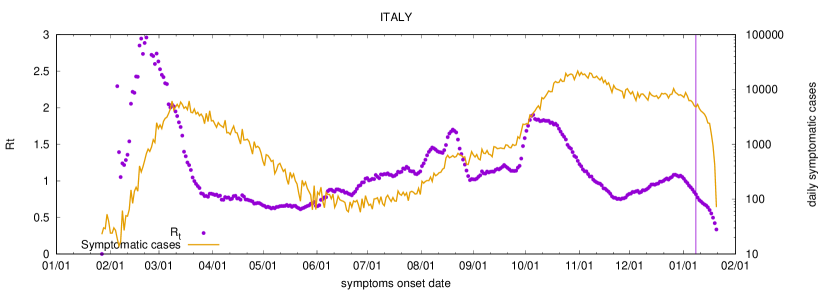
Figure 1: Number of symptomatic cases in Italy per day reported by date of onset of symptoms (right axis, log scale) and $R_{t}$ (left axis, linear scale) obtained using Eq.(6) and then averaged over a week. The vertical line indicates the most recent data reported as consolidated.

Now we turn to Fig.2 and Fig.3. For each country we plot the value of $R^{(k)}_{t}$ for its regions versus time and $R_{t}/\langle{R_{0}}(t)\rangle$ versus $c(t)$ along with the best fit for $\lambda$. The fit was performed neglecting the first $100$ days of the epidemic when testing was quite irregular and the number of PCR tests extremely low. The error on $\lambda$ was evaluated by changing this threshold from $50$ to $150$ days.

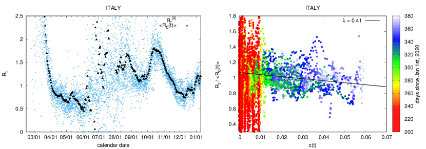
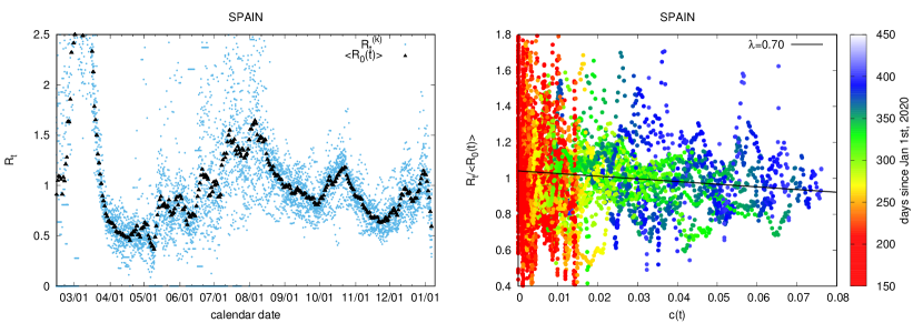
Figure 2: (Color online) estimation results for Italy, France, and Spain. (Left panel) scatterplot of $R_{t}$ evaluated for all the regions together with $\langle R_{0}(t)\rangle$. For the Italian data notice that, except for summer, $R_{t}$ evaluated on standard data is quite like that evaluated on the ISS data reporting cases by date of onset of symptoms. (Right panel) The fluctuations of $R_{t}^{(k)}/\langle R_{0}(t)\rangle$ vs $c(t)$ with the best linear fit leading the estimate of $\lambda$. Color indicates date in days from Jan. $1^{\text{st}}$, 2020.

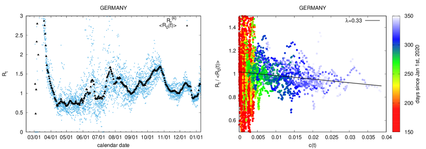
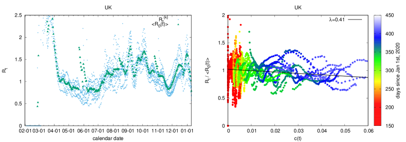
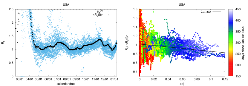
Figure 3: (Color online) estimation results for Germany, UK, and USA. (Left panel) scatterplot of $R_{t}$ evaluated for all the regions together with $\langle R_{0}(t)\rangle$. (Right panel) The fluctuations of $R_{t}^{(k)}/\langle R_{0}(t)\rangle$ vs $c(t)$ with the best linear fit leading the estimate of $\lambda$. The color shows the date as days from Jan. $1^{\text{st}}$, 2020.

A straightforward application of the estimate of the true number of infections is to adjust the case fatality rate (CFR) to better approximate the infectious fatality rate (IFR). The CFR is defined as the number of reported deaths per number of reported cases. It approximates IFR, which is an estimate of the death rate among all those infected with SARS-CoV-2, the virus that causes CoViD-19. In table 2 we estimate the unrecorded fraction of the true number of infected individuals as well as the corrected value of the case fatality rate ($\lambda$-CFR). This correction does not capture every reason the CFR can differ from the IFR. Some additional differences are due to delayed effects, population age, typical medical conditions of the population, and healthcare system efficiency.

Country	$\lambda$	C.I.	CFR (%)	$\lambda$-CFR (%)
Italy	$0.35$	$[0.31,0.42]$	$3.52$	$1.23$
France	$0.39$	$[0.34,0.46]$	$2.45$	$0.95$
Germany	$0.33$	$[0.31,0.41]$	$2.10$	$0.69$
Spain	$0.70$	$[0.63,0.84]$	$2.74$	$1.92$
UK	$0.41$	$[0.37,0.49]$	$2.70$	$1.11$
USA	$0.62$	$[0.56,0.74]$	$1.70$	$1.05$

Table 2: Results of the testing variable estimation as for January 2021.

As the vaccination campaign continues, we must consider the effects of immunization through vaccination on our analysis. The functional form will change to $R_{t}/\langle R_{0}\rangle\sim\left(1-{c(t)}/{\lambda}\right)\left(1-\nu(t)\right)\simeq\left(1-{c(t)}/{\lambda}-\nu(t)\right)$, where new term takes in account the vaccinated fraction of the population $\nu(t)$. If data on the vaccination campaign are available at the regional level, and $\nu(t)$ reaches a substantial value, one should perform a two-dimensional fit of $R_{t}/\langle R_{0}\rangle$ as a function of $c(t)$ and $v(t)$. The slope of the iso-$R_{t}/\langle R_{0}\rangle$ lines, i.e., the lines in the $c(t)-v(t)$ plane of constant $R_{t}/\langle R_{0}\rangle$, will give another estimate of $\lambda$. This will allow us to compare and contrast the effects of vaccination and new infectious cases on $R_{t}$. If $\lambda\simeq 1$, their effects should be the same. If $\lambda<1$, we expect that the effect of a given number of infectious individuals on $R_{t}$ to be larger than that of the same number of vaccinated.

Robustness check using seroprevalence data

Our findings can be checked by comparing our results with alternative methods used to evaluate the true number of people that have had SARS-CoV-2. One of the most reliable methods is the analysis of seroprevalence of IgG antibodies in blood. We compare our $\lambda$ values with those obtained by two papers [26, 27] and a dashboard on an official website [28].

In particular, [26] reports the fraction of people showing IgG antibodies to SARS-CoV-2 over the number of officially reported cases as of the end of May $2020$. This ratio should be compared with $\lambda^{-1}$. In Table 3 of [26] data for 10 sites are reported. They range from a minimum of $6.0$ for Connecticut to a maximum of $23.8$ for Missouri. The worst hit state, New York, has a value of $11.9$. In Fig.4 (left panel), we report the value of $\lambda$ using data covering the same period, namely ending May $23^{\text{rd}}$, $2020$. We report our best fit yielding $\lambda=0.06$, together with the line corresponding to the $\lambda$ obtained from serological data described in [26]. The same approach was followed in Fig.4 (right panel), where we report the typical value retrieved from [28] (between 6 and 7 times the official number of cases) with our fit at the date of the last update of the website (July $2020$).

Passing from late spring to the end of summer, $\lambda$ increased considerably. This effect is apparent in the dashboard data [28] and the same pattern holds in all countries analyzed. We presume this increase is due to increased testing ability and contact tracing efforts made in all countries. Nevertheless, as a final remark, we stress that if our results are confirmed, in all countries the tracing capacity is not enough, by itself, to mitigate the spread of SARS-CoV-2. Due to the large contribution of asymptomatic or mild-symptomatic cases, we think that reaching a value of $\lambda\simeq 1$ would be necessary. This would require a massive use of tests as seen, for example, in China during its prevention of a second wave.

Finally, in comparing our approach to the seroprevalence data, we found that our method gives results that are of the same order of magnitude. Our method tends to overestimate the serological results. This could be mark against our approach, but one should note that seroprevalence-based infection estimates are conservative [28]. Some studies have found that infected persons who are asymptomatic or have mild symptoms do not have detectable antibodies. Other studies found that antibody levels decrease and become undetectable in some patients over time (see, for example, [29, 30]). Another explanation of this overestimation is that the number of susceptible individuals is not the entire population due to cross-immunity with other common coronaviruses [31, 32, 33].

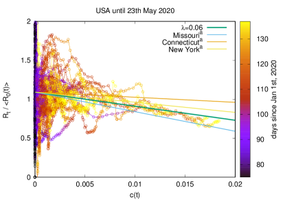
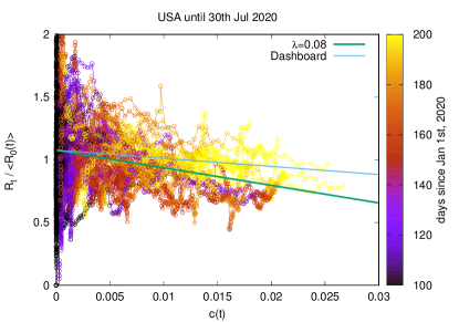
Figure 4: (left panel, color online) best fit value for $\lambda$ through May $23^{\text{rd}}$, 2020 compared with $\lambda^{a}$ obtained from Table 3 of [26] for New York ($\lambda=11.9$) and for the extremal cases of Missouri ($\lambda=1/23.8$) and Connecticut ($\lambda=1/6.0$). (Right panel, color online) same approach as in the left panel with data ending July $30^{\text{th}}$, 2020 compared with the average value given by [28] ($\lambda=1/6$)

4 Conclusions

Knowledge of true prevalence of CoViD-19 is critical for informing policy decisions about how to distribute resources and manage the impacts of CoViD-19 on public health, society and the economy[34, 35]. The true scale of the epidemic can affect economic development since it reduces long-run economic growth by limiting the size of social networks. On the contrary a low prevalence estimate could lead people to take more epidemic-relevant risks, making disease eradication impossible using social distancing policies only.

We have proposed a method to estimate the true number of infected people, unveiling the true scale of CoViD-19 by using PCR test data alone.We the used this method to estimate a more reliable case fatality rate. Our approach is a phenomenological estimate of the true scale of the epidemic, since it is based on an empirical relationship between phenomena, in a way which is consistent with fundamental theory, but is not directly derived from that theory. Consequently, our method can be affected by errors which we are not able to distinguish from the lack of theoretical understanding. Nevertheless, there are two remarkable results. The few attempts to assesss the true impact of SARS-CoV-2 via serological tests yield $\lambda$-values comparable in order of magnitude with our calculations [36]. Moreover, countries that performed better tracing, like the USA, experienced a fatality rate lower than Italy, France, and Spain (in the first wave). Improved contact tracing performance (higher $\lambda$) leads to a lower fatality rate because the rate is calculated using the correct denominator. Good contact tracing can also help keep the epidemic under control, preventing the virus from reaching fragile and elderly people. Thus leading to a bona fide decrease in the fatality rate.

We have proposed that the study of the graph $R_{t}$ vs $c(t)$ and $R_{t}/\langle{R_{0}}(t)\rangle$ vs $c(t)$ can provide useful insight into epidemic dynamics. These methods should be useful in other epidemics with incomplete data due to the presence of unrecorded contagious individuals, for example, the seasonal flu. Minor modifications allow this approach to keep its effectiveness even in the presence of active vaccination campaigns. By contributing to a better-informed response to epidemics, we believe this work serves to benefit society as a whole.

5 Acknowledgments

Fabio Vanni acknowledges support from the European Union’s Horizon 2020 research and innovation programme under grant agreement No.822781 GROWINPRO - Growth Welfare Innovation Productivity.

6 Conflict of interest

The authors declare that there are no conflicts of interest regarding the publication of this paper.

Bibliography

- [1] Eric A Meyerowitz, Aaron Richterman, Isaac I Bogoch, Nicola Low, and Muge Cevik. Towards an accurate and systematic characterisation of persistently asymptomatic infection with sars-cov-2. The Lancet Infectious Diseases, 2020.
- [2] Seyed M Moghadas, Meagan C Fitzpatrick, Pratha Sah, Abhishek Pandey, Affan Shoukat, Burton H Singer, and Alison P Galvani. The implications of silent transmission for the control of covid-19 outbreaks. Proceedings of the National Academy of Sciences, 117(30):17513–17515, 2020.
- [3] Mathias Peirlinck, Kevin Linka, Francisco Sahli Costabal, and Ellen Kuhl. Outbreak dynamics of covid-19 in china and the united states. Biomechanics and modeling in mechanobiology, page 1, 2020.
- [4] Stephen A Lauer, Kyra H Grantz, Qifang Bi, Forrest K Jones, Qulu Zheng, Hannah R Meredith, Andrew S Azman, Nicholas G Reich, and Justin Lessler. The incubation period of coronavirus disease 2019 (covid-19) from publicly reported confirmed cases: estimation and application. Annals of internal medicine, 172(9):577–582, 2020.
- [5] Andrew William Byrne, David McEvoy, Aine B Collins, Kevin Hunt, Miriam Casey, Ann Barber, Francis Butler, John Griffin, Elizabeth A Lane, Conor McAloon, Kirsty O’Brien, Patrick Wall, Kieran A Walsh, and Simon J More. Inferred duration of infectious period of sars-cov-2: rapid scoping review and analysis of available evidence for asymptomatic and symptomatic covid-19 cases. BMJ Open, 10, 08 2020.
- [6] Seth Flaxman, Swapnil Mishra, Axel Gandy, H Juliette T Unwin, Thomas A Mellan, Helen Coupland, Charles Whittaker, Harrison Zhu, Tresnia Berah, Jeffrey W Eaton, et al. Estimating the effects of non-pharmaceutical interventions on covid-19 in europe. Nature, 584(7820):257–261, 2020.
- [7] Ruiyun Li, Sen Pei, Bin Chen, Yimeng Song, Tao Zhang, Wan Yang, and Jeffrey Shaman. Substantial undocumented infection facilitates the rapid dissemination of novel coronavirus (sars-cov-2). Science, 368(6490):489–493, 2020.
- [8] Jason Oke and Carl Heneghan. Global covid-19 case fatality rates. cebm. 2020. https://www.cebm.net/covid-19/global-covid-19-case-fatality-rates/.
- [9] Steven J Phipps, R Quentin Grafton, and Tom Kompas. Robust estimates of the true (population) infection rate for covid-19: a backcasting approach. Royal Society Open Science, 7(11):200909, 2020.
- [10] Christophe Fraser. Estimating individual and household reproduction numbers in an emerging epidemic. PloS one, 2(8):e758, 2007.
- [11] Katelyn M Gostic, Lauren McGough, Edward B Baskerville, Sam Abbott, Keya Joshi, Christine Tedijanto, Rebecca Kahn, Rene Niehus, James A Hay, Pablo M De Salazar, et al. Practical considerations for measuring the effective reproductive number, r t. PLoS computational biology, 16(12):e1008409, 2020.
- [12] Hiroshi Nishiura. Time variations in the generation time of an infectious disease: implications for sampling to appropriately quantify transmission potential. Mathematical Biosciences & Engineering, 7(4):851–869, 2010.
- [13] David Champredon, Jonathan Dushoff, and David JD Earn. Equivalence of the erlang-distributed seir epidemic model and the renewal equation. SIAM Journal on Applied Mathematics, 78(6):3258–3278, 2018.
- [14] D Breda, O Diekmann, WF De Graaf, A Pugliese, and R Vermiglio. On the formulation of epidemic models (an appraisal of kermack and mckendrick). Journal of biological dynamics, 6(sup2):103–117, 2012.
- [15] Anne Cori, Neil M Ferguson, Christophe Fraser, and Simon Cauchemez. A new framework and software to estimate time-varying reproduction numbers during epidemics. American journal of epidemiology, 178(9):1505–1512, 2013.
- [16] Seth Flaxman, Swapnil Mishra, Axel Gandy, H Unwin, H Coupland, T Mellan, H Zhu, T Berah, J Eaton, P Perez Guzman, et al. Report 13: Estimating the number of infections and the impact of non-pharmaceutical interventions on covid-19 in 11 european countries, 2020.
- [17] DPC. Covid-19 italia, 2020. Sito del Dipartimento della Protezione Civile - Presidenza del Consiglio dei Ministri, https://github.com/pcm-dpc/COVID-19.
- [18] ISS. Integrated surveillance of covid-19 in italy, 2020. Scientific coordination by Centro Nazionale per la Prevenzione delle malattie e la Promozione della Salute, CNAPPS - ISS,https://www.epicentro.iss.it/en/coronavirus.
- [19] Santé publique France. Taux d’incidence de l’épidémie de covid-19, 2020. available at https://www.data.gouv.fr/fr/organizations/sante-publique-france/.
- [20] Ministerio de Sanidad. Enfermedad por nuevo coronavirus, covid-19, 2020. available at https://www.mscbs.gob.es/profesionales/saludPublica/ccayes/alertasActual/nCov/situacionActual.htm.
- [21] DATADISTA. Coronavirus disease 2019 (covid-19) in spain, 2020. available at https://github.com/datadista/datasets/tree/master/COVID%2019.
- [22] Robert Koch-Institut. Covid-19 reports, 2020. available at https://www.rki.de/EN/Content/infections/epidemiology/outbreaks/COVID-19/COVID19.html.
- [23] Center for Disaster Management Risklayer GmbH and Risk Reduction Technology (CEDIM). Covid-19 case numbers for germany, 2020. available at https://github.com/jgehrcke/covid-19-germany-gae.
- [24] Gov.UK. Covid-19 in the uk, 2020. available at https://coronavirus.data.gov.uk/details/download.
- [25] CovidTracking. The covid tracking project, 2020. available at https://covidtracking.com/data/api.
- [26] Fiona P Havers, Carrie Reed, Travis Lim, Joel M Montgomery, John D Klena, Aron J Hall, Alicia M Fry, Deborah L Cannon, Cheng-Feng Chiang, Aridth Gibbons, et al. Seroprevalence of antibodies to sars-cov-2 in 10 sites in the united states, march 23-may 12, 2020. JAMA internal medicine, 180(12):1576–1586, 2020.
- [27] Kristina L Bajema, F Scott Dahlgren, Travis W Lim, Nicolette Bestul, Holly M Biggs, Jacqueline E Tate, Claudio Owusu, Christine M Szablewski, Cherie Drenzek, Jan Drobeniuc, et al. Comparison of estimated sars-cov-2 seroprevalence through commercial laboratory residual sera testing and a community survey. Clinical Infectious Diseases, 2020.
- [28] Centers for Disease Control and Prevention. Commercial laboratory seroprevalence survey data. available at https://covid.cdc.gov/covid-data-tracker/#national-lab, 2020-01-04.
- [29] Nina Le Bert, Anthony T Tan, Kamini Kunasegaran, Christine YL Tham, Morteza Hafezi, Adeline Chia, Melissa Hui Yen Chng, Meiyin Lin, Nicole Tan, Martin Linster, et al. Sars-cov-2-specific t cell immunity in cases of covid-19 and sars, and uninfected controls. Nature, 584(7821):457–462, 2020.
- [30] Kevin Ng, Nikhil Faulkner, Georgina Cornish, Annachiara Rosa, Christopher Earl, Antoni Wrobel, Donald Benton, Chloe Roustan, William Bolland, Rachael Thompson, et al. Pre-existing and de novo humoral immunity to sars-cov-2 in humans. BioRxiv, 2020.
- [31] Marc Lipsitch, Yonatan H Grad, Alessandro Sette, and Shane Crotty. Cross-reactive memory t cells and herd immunity to sars-cov-2. Nature Reviews Immunology, 20(11):709–713, 2020.
- [32] Kevin W. Ng, Nikhil Faulkner, Georgina H. Cornish, Annachiara Rosa, Ruth Harvey, Saira Hussain, Rachel Ulferts, Christopher Earl, Antoni G. Wrobel, Donald J. Benton, Chloe Roustan, William Bolland, Rachael Thompson, Ana Agua-Doce, Philip Hobson, Judith Heaney, Hannah Rickman, Stavroula Paraskevopoulou, Catherine F. Houlihan, Kirsty Thomson, Emilie Sanchez, Gee Yen Shin, Moira J. Spyer, Dhira Joshi, Nicola O Reilly, Philip A. Walker, Svend Kjaer, Andrew Riddell, Catherine Moore, Bethany R. Jebson, Meredyth Wilkinson, Lucy R. Marshall, Elizabeth C. Rosser, Anna Radziszewska, Hannah Peckham, Coziana Ciurtin, Lucy R. Wedderburn, Rupert Beale, Charles Swanton, Sonia Gandhi, Brigitta Stockinger, John McCauley, Steve J. Gamblin, Laura E. McCoy, Peter Cherepanov, Eleni Nastouli, and George Kassiotis. Preexisting and de novo humoral immunity to sars-cov-2 in humans. Science, 2020.
- [33] Peter Doshi. Covid-19: Do many people have pre-existing immunity? Bmj, 370, 2020.
- [34] Organisation for Economic Co-operation and Development (OECD). The territorial impact of covid-19: managing the crisis across levels of government, 2020.
- [35] Joshua S Gans. The economic consequences of r= 1: Towards a workable behavioural epidemiological model of pandemics. National Bureau of Economic Research Working Paper Series, 2020.
- [36] Linda Laura Sabbadini, Maria Clelia Romano, and Orietta Luzi. Istat (august 03,2020) primi risultati indagine di sieroprevalenza sul sarscov2, 2020. retrieved from https://www.istat.it/it/archivio/246156.