A Dimension-free Computational Upper-bound for Smooth Optimal Transport Estimation

Abstract

It is well-known that plug-in statistical estimation of optimal transport suffers from the curse of dimensionality. Despite recent efforts to improve the rate of estimation with the smoothness of the problem, the computational complexity of these recently proposed methods still degrade exponentially with the dimension. In this paper, thanks to an infinite-dimensional sum-of-squares representation, we derive a statistical estimator of smooth optimal transport which achieves a precision $\varepsilon$ from $\tilde{O}(\varepsilon^{-2})$ independent and identically distributed samples from the distributions, for a computational cost of $\tilde{O}(\varepsilon^{-4})$ when the smoothness increases, hence yielding dimension-free statistical and computational rates, with potentially exponentially dimension-dependent constants.

1 Introduction

The comparison between probability distributions is a fundamental task and has been extensively used in machine learning. For this purpose, optimal transport (OT) has recently gained traction in different subfields of machine learning (ML), such as natural language processing (NLP) (Xu et al., 2018; Chen et al., 2018), generative modeling (Arjovsky et al., 2017; Tolstikhin et al., 2018; Salimans et al., 2018), multi-label classification (Frogner et al., 2015), domain adaptation (Redko et al., 2019), clustering (Ho et al., 2017), and has had an impact in other areas such as imaging sciences (Feydy et al., 2017; Bonneel et al., 2011). Indeed, OT is a tool to compare data distributions which has arguably many more geometric properties than other available divergences (Peyré and Cuturi, 2019).

In practice, the optimal transport cost is often computed for the squared distance (leading to the Wasserstein-2 distance) on sampled distributions with $n$ observations, and it is well-known that optimal transport suffers from the curse of dimensionality (Fournier and Guillin, 2015): the plug-in strategy, which simply consists in computing the Wasserstein distance between the sampled distributions, yields an estimation of the Wasserstein squared distance between a density and its sampled version in $O(1/n^{1/d})$, which degrades rapidly in high dimensions; this can only be improved to $O(1/n^{2/d})$ in the case of two different distributions (Chizat et al., 2020).

However, high dimension is the usual setting in machine learning, such as in NLP (Grave et al., 2019), and even if the intrinsic dimensionality of data can be leveraged (Weed and Bach, 2019; Niles-Weed and Rigollet, 2019), poor theoretical rates of convergence are a recurrent feature of OT. Liang (2018, 2019) recently showed that when the measures admit smooth densities, the Wasserstein-1 distance (as part of a more general class of integral probability metrics (IPM)) those minimax sample complexity rates could be improved to almost $O(1/\sqrt{n})$ when the smoothness increases. Weed and Berthet (2019) then showed equivalent rates in the case smooth densities with geometric assumptions on their supports for the Wasserstein-$p$ distances with $p>1$, which are not IPMs, and proposed a corresponding estimator based on a dedicated non-polynomial-time algorithm. Matching rates were then proved for the transportation maps themselves (Hütter and Rigollet, 2019) in the Wasserstein-2 setting, under smoothness assumptions on those maps. This line of work is deeply related to the regularity theory of optimal transport, that guarantees the smoothness of the optimal map in Euclidean spaces under similar assumptions on the source and target distributions, and their supports (Caffarelli, 1992; De Philippis and Figalli, 2014). Yet, to this day no practically tractable algorithm (e.g., with polynomial time) matching the bounds of Weed and Berthet (2019) and Hütter and Rigollet (2019) is known.

State of the art.

An approach that has first been advocated in the machine learning community as a way to efficiently approximate empirical OT and to make it differentiable consists in adding an entropic regularization term to the OT problem (Cuturi, 2013). Rates on the sample complexity of entropic optimal transport have then been studied by Genevay et al. (2019) and Mena and Niles-Weed (2019), and were proven to be of the order $O(\frac{1}{\varepsilon^{\lfloor d/2\rfloor}\sqrt{n}})$, for small values of $\varepsilon$. Although the dependency in the number of samples is in $1/\sqrt{n}$, the constant degrades exponentially with respect to the dimension. Entropic OT and Sinkhorn divergences (Genevay et al., 2018) were then leveraged as a tool to study the sample complexity of the (unregularized) OT problem itself: the most advanced results in this direction were derived by Chizat et al. (2020), who show that with few assumptions on the regularity of the Kantorovich potentials, the squared Wasserstein distance can be estimated using $O(\varepsilon^{-d/2+2})$ samples and $\tilde{O}(\varepsilon^{-(d^{\prime}+5.5)})$ operations (with $d^{\prime}=2\lfloor\frac{d}{2}\rfloor$) with high probability.

Our work can be related to a current research direction which consists in developing estimators of the Wasserstein distance for classes of smooth distributions, with smoothness parameter $m$, that have better performances than in the general case. Related to this trend, Liang (2018, 2019) showed minimax rates for a class of integral probability metrics (IPM) that includes the Wasserstein-1 distance, as a function of the smoothness of the distributions. However, (i) for $p>1$, the Wasserstein-$p$ distance $W_{p}$ is not an IPM and (ii) no estimators with matching rates are proposed in those two works. So far, two main contributions leveraging smoothness that are applicable to the $W_{2}$ distance can be found. Hütter and Rigollet (2019) derive minimax rates for the estimation of the OT maps and propose an estimator which necessitates, for an $L_{2}$ error on the maps of order $\varepsilon$, $O(\varepsilon^{-\frac{2m-1+d/2}{2m}})$ samples. While statistically almost optimal, this estimator is not computationally feasible as it requires to project the potentials on a space of smooth, strongly-convex functions. Instead, Weed and Berthet (2019) derive estimators for the densities requiring $O(\varepsilon^{-\frac{d+2m}{1+m}})$ samples and, under the assumption that an efficient resampler is available, derive an estimator of the OT distance that can be calculated in $\tilde{O}(\varepsilon^{-(2d+d/2)})$ time.

While the contributions above do succeed in taking advantage of the smoothness from a statistical point of view, they do not manage to take advantage of the smoothness from a computational point of view. Actually, statistical-computational gaps are known to exist for some instances of high-dimensional OT, such as the spiked transport model of Niles-Weed and Rigollet (2019).

Contributions.

In this paper, we bridge the statistical-computational gap of smooth OT estimation and we provide a positive answer to the question whether smoothness of the optimal potentials can be computationally beneficial to an efficient statistical estimator. More precisely, we propose an algorithm which, for a given accuracy $\varepsilon$, needs $O(\varepsilon^{-2})$ samples and has a computational complexity of $\tilde{O}(\varepsilon^{-\max(4,\frac{7d}{m-d})})$. Note that the computational complexity improves with the regularity of the distributions and, when $m\geq 3d$, it is $\tilde{O}(\varepsilon^{-4})$, i.e., independent of the dimension $d$ in the exponent (but not in the constants). We thus show that smoothness can be leveraged in the computational estimation of optimal transport.

Moreover, we consider different scenarios beyond i.i.d. sampling, such as the case where we are able to compute exact integrals or where we can evaluate the densities in given points, by representing the problem in terms of kernel mean embeddings (Muandet et al., 2017). This allows to make a unified analysis for all the cases. The total error is then the sum of the error induced by approximating via the kernel mean embedding plus the error induced by subsampling the constraints. Interestingly, in the other scenarios the computational cost to achieve an error $\varepsilon$ can be smaller than $\varepsilon^{-4}$, as reported below. This is particularly interesting in the case we can evaluate the densities in given points and avoids using expensive Monte-Carlo sampling techniques to obtain i.i.d. samples (see Section 6 for more details). Our results are summarized below.

Theorem 1.1.

Let $\varepsilon>0$. Let $\mu,\nu$ satisfy 1 for some $m>d$. Let $\widehat{\text{OT}}$ be the proposed estimator defined in Eq. 6 and computed as in Appendix F with the same parameters as in Corollary 2.2. The cost to achieve $|\widehat{\text{OT}}-\text{OT}(\mu,\nu)|\leq\varepsilon$ for the three scenarios is:

1. (Exact integral) Time: $\tilde{O}(\varepsilon^{-\frac{7d}{m-d}})$. Space: $\tilde{O}(\varepsilon^{-\frac{4d}{m-d}})$.

2. (Evaluation) Time: $\tilde{O}(\varepsilon^{-\frac{7d}{m-d}})$. Space: $\tilde{O}(\varepsilon^{-\frac{4d}{m-d}})$. $\#$evaluations of $\mu,\nu$: $\tilde{O}(\varepsilon^{-\frac{d}{m+1}})$.

3. (Sampling) Time: $\tilde{O}(\varepsilon^{-\max(4,\frac{7d}{m-d})})$. Space: $\tilde{O}(\varepsilon^{-\frac{4d}{m-d}})$. $\#$samples of $\mu,\nu$: $\tilde{O}(\varepsilon^{-2})$.

The second key contribution of this paper is to provide a new representation theorem for solutions of smooth optimal transport. The inequality constraint in the dual OT problem can be replaced with an equality constraint involving a finite sum-of-squares in a Sobolev space. In comparison with Rudi et al. (2020), it is a non-trivial extension of their representation result to the case of a continuous set of global minimizers instead of a finite set.

2 Sketch of the result and derivation of the algorithm

In this paper, we consider the optimal transport problem for the quadratic cost on bounded subsets $X,Y$ of the Euclidean space $\mathbb{R}^{d}$. The set of probability measures on $X$ is denoted by $\mathcal{P}(X)$. The optimal transport problem with quadratic cost $c(x,y)=\frac{1}{2}\|x-y\|^{2}$ can be stated in its dual formulation as

$$\begin{split}\text{OT}(\mu,\nu)=\sup_{u,v\in C(\mathbb{R}^{d})}~{}&~{}~{}\int u(x)d\mu(x)+\int v(y)d\nu(y)\\ \textrm{subject to}~{}&~{}~{}c(x,y)\geq u(x)+v(y),~{}~{}\forall(x,y)\in X\times Y,\end{split}$$ (1)

As a standard result in optimal transport theory, the supremum is attained and the functions $u_{\star},v_{\star}$ are referred to as the Kantorovich potentials (see Santambrogio, 2015).

The proposed approach to approximate $\text{OT}(\mu,\nu)$ is the result of two main ingredients: (1) a suitable way to represent smooth functions and to approximate their integral in $\mu,\nu$, (2) a way to enforce efficiently the dense set of constraints on $u,v$.

Preliminary step: Representing smooth functions and integrals.

We represent smooth functions via a reproducing Kernel Hilbert space (RKHS) (Aronszajn, 1950; Steinwart and Christmann, 2008), for which functions can be represented as linear forms. In Section 4 we show that under smoothness assumptions on $\mu$ and $\nu$ (1) we have $u\in{{\mathcal{H}}_{X}}$ and $v\in{{\mathcal{H}}_{Y}}$ where ${{\mathcal{H}}_{X}}$ and ${{\mathcal{H}}_{Y}}$ are two suitable RKHSs on $X$ and $Y$, associated with two bounded continuous feature maps $\phi_{X}:X\to{{\mathcal{H}}_{X}}$ and $\phi_{Y}:Y\to{{\mathcal{H}}_{Y}}$. Note that RKHSs offer several advantages. First, leveraging the reproducing property, we can represent the integrals in the functional of Eq. 1 as inner products in terms of the kernel mean embeddings $w_{\mu}\in{{\mathcal{H}}_{X}}$ and $w_{\nu}\in{{\mathcal{H}}_{Y}}$ where $w_{\mu}=\int_{X}\phi_{X}(x)d\mu(x)$ and $w_{\nu}=\int_{Y}\phi_{Y}(y)d\nu(y)$. Indeed, by the reproducing property, for all $u\in{{\mathcal{H}}_{X}}$, we have:

$$\int_{X}u(x)d\mu(x)=\int_{X}\langle u,\,\phi_{X}(x)\rangle_{{\mathcal{H}}_{X}}d\mu(x)=\big{<}u,\int_{X}\phi_{X}(x)d\mu(x)\big{>}_{{\mathcal{H}}_{X}}=\langle u,\,w_{\mu}\rangle_{{\mathcal{H}}_{X}},$$

and the same reasoning holds for the integral on $\nu$, i.e., $\int_{Y}v(y)d\nu(y)=\langle v,\,w_{\nu}\rangle_{{\mathcal{H}}_{Y}}$, for all $v\in{{\mathcal{H}}_{Y}}$. This construction is known as kernel mean embedding (Muandet et al., 2017). Moreover, RKHSs allow the so-called kernel trick (Steinwart and Christmann, 2008), i.e., to express the resulting algorithm in terms of kernel functions that in our case correspond to $k_{X}(x,x^{\prime})=\langle\phi_{X}(x),\,\phi_{X}(x^{\prime})\rangle_{{\mathcal{H}}_{X}}$ and $k_{Y}(y,y^{\prime})=\langle\phi_{Y}(y),\,\phi_{Y}(y^{\prime})\rangle_{{\mathcal{H}}_{Y}}$, that are known explicitly and are easily computable in $O(d)$.

The main step: Dealing with a dense set of inequalities.

Even assuming that we are able to compute integrals in closed form and restricting to $m$-times differentiable $u,v$, the main challenge is to deal with the dense set of inequalities $c(x,y)\geq u(x)+v(y)$ that $u,v$ must satisfy, for any $(x,y)\in X\times Y$. Indeed, an intuitive approach would be to subsample the set, i.e., to take $\ell$ points $(\tilde{x}_{1},\tilde{y}_{1}),\dots,(\tilde{x}_{\ell},\tilde{y}_{\ell})$ in $X\times Y$ and consider only the constraints $c(\tilde{x}_{j},\tilde{y}_{j})\geq u(\tilde{x}_{j})+v(\tilde{y}_{j})$ for $j=1,\dots,\ell$. This approach, however, is only able to leverage the Lipschitzianity of $u,v$ (Aubin-Frankowski and Szabo, 2020) and leads to an error in the order of $\ell^{-1/d}$ that does not allow to break the dependence in $d$ in the exponent, and yields rates that are equivalent to the plugin estimator.

In this paper, we leverage a more refined technique to approximate the dense set of inequalities, introduced by Rudi et al. (2020) for the problem of non-convex optimization, and that allows to break the curse of dimensionality for smooth problems. The idea behind this technique is the consideration that, while a dense set of inequalities is poorly approximated by subsampling, the situation is different in the case of a dense set of equality constraints, for which an optimal rate of $O(\ell^{-m/d})$ is achievable for $m$-times differentiable constraints (Wendland and Rieger, 2005). The construction works in two steps: first, substitute the inequality constraints with equality constraints that are equivalent, and then subsample. In the next two paragraphs we explain how to apply this approach to the problem of OT.

Removing the inequalities: positive definite operator characterization.

To apply the construction recalled above to our scenario, we first consider the following problem. Let ${{\mathcal{H}}_{XY}}$ be a Hilbert space on $X\times Y$ and $\phi:X\times Y\to{{\mathcal{H}}_{XY}}$. Denote by $k_{XY}$ the kernel $k_{XY}((x,y),(x^{\prime},y^{\prime}))=\langle\phi(x,y),\,\phi(x^{\prime},y^{\prime})\rangle_{{\mathcal{H}}_{XY}}$ for any $(x,y),(x^{\prime},y^{\prime})\in X\times Y$ and by $\mathbb{S}_{+}({{{\mathcal{H}}_{XY}}})$ the space of positive operators on ${{\mathcal{H}}_{XY}}$. We define

$$\begin{split}\max_{\begin{subarray}{c}u\in{{\mathcal{H}}_{X}},v\in{{\mathcal{H}}_{Y}},\\ A\in\mathbb{S}_{+}({{{\mathcal{H}}_{XY}}})\end{subarray}}~{}~{}~{}&\langle u,\,w_{\mu}\rangle_{{\mathcal{H}}_{X}}+\langle v,\,w_{\nu}\rangle_{{\mathcal{H}}_{Y}}\\ \textrm{subject to}~{}~{}~{}&\forall(x,y)\in X\times Y,~{}~{}~{}c(x,y)-u(x)-v(y)=\langle\phi(x,y),\,A\phi(x,y)\rangle_{{\mathcal{H}}_{XY}},\end{split}$$ (2)

where the inequality in (1) is substituted with an equality w.r.t. a positive definite operator $A$ on ${{\mathcal{H}}_{XY}}$. Note that Problem (1) is a relaxation of Problem (2): indeed, if for a given pair $u\in{{\mathcal{H}}_{X}},v\in{{\mathcal{H}}_{Y}}$ there exists a positive definite $A$ satisfying the equality above, then

$$c(x,y)-u(x)-v(y)=\langle\phi(x,y),\,A\phi(x,y)\rangle_{{\mathcal{H}}_{XY}}\geq 0,\qquad\forall(x,y)\in X\times Y,$$

so the couple $(u,v)$ is admissible for (1). However, even for an admissible couple in (1) satisfying $u\in{{\mathcal{H}}_{X}},v\in{{\mathcal{H}}_{Y}}$, a positive operator $A$ may not exist. Indeed, note that the technique of representing a positivity constraint in terms of a positive matrix has a long history in the community of polynomial optimization (Lasserre, 2001; Parrilo, 2003; Lasserre, 2009), which shows that in general the resulting problem is not equivalent to the original one, for any chosen degree of polynomial approximation. This fact leads to the so-called sum of squares hierarchies, also used for optimal transport (Henrion and Lasserre, 2020). Instead, using kernels, Rudi et al. (2020) showed that there exists a positive operator with finite rank that matches the constraints and makes the two problems equivalent, when the constraint is attained on a finite set of points. However, such existence results cannot be used for the problem in (2), since in the case of optimal transport the set of zeros corresponds to the graph of the optimal transport map and is a smooth manifold, when $\mu,\nu$ are smooth (De Philippis and Figalli, 2014).

A crucial point of our contribution is then to prove that, with a quadratic cost $c(x,y)=\frac{1}{2}\|x-y\|^{2}$ and under the same assumptions on the densities and their supports, or under smoothness assumptions on the Kantorovich potentials, there exists a positive operator on a suitable Hilbert space that represents the function $c(x,y)-u(x)-v(y)$ for a pair $u,v$ maximizing (1), making the two problems equivalent. The result is reported in Theorem 4.1. The proof is derived using the Fenchel dual characterization of $u_{\star},v_{\star}$ and gives a sharp control of the rank of $A$.

Subsampling the constraints and approximating the integrals.

We restrict the constraint of (2) to $(\tilde{x}_{1},\tilde{y}_{1}),\dots,(\tilde{x}_{\ell},\tilde{y}_{\ell})\subset X\times Y$ for $\ell\in\mathbb{N}$. However, we need to add a penalization for $u,v$ and $A$ to avoid overfitting, since the error induced by subsampling the constraints is proportional to the trace of $A$ (Rudi et al., 2020) and, in our case, also to the norms of $u,v$, as derived in Theorem 5.2 in Section 5. Finally, in two of the three scenarios of interest for the paper, i.e., (i) when we can only evaluate $\mu,\nu$ pointwise, or (ii) when we have only i.i.d. samples from $\mu,\nu$, we do not have access to the kernel mean embeddings $w_{\mu}\in{{\mathcal{H}}_{X}},w_{\nu}\in{{\mathcal{H}}_{Y}}$. Therefore, we need to use some estimators $\hat{w}_{\mu}\in{{\mathcal{H}}_{X}},\hat{w}_{\nu}\in{{\mathcal{H}}_{Y}}$ that are derived in Section 6. The resulting problem is the following, for some regularization parameters $\lambda_{1},\lambda_{2}>0$:

$$\begin{split}\max_{\begin{subarray}{c}u\in{{\mathcal{H}}_{X}},v\in{{\mathcal{H}}_{Y}},\\ A\in\mathbb{S}_{+}({{{\mathcal{H}}_{XY}}})\end{subarray}}~{}~{}~{}&\langle u,\,\hat{w}_{\mu}\rangle_{{\mathcal{H}}_{X}}+\langle v,\,\hat{w}_{\nu}\rangle_{{\mathcal{H}}_{Y}}-\lambda_{1}\mathrm{Tr}(A)-\lambda_{2}(\|u\|^{2}_{{\mathcal{H}}_{X}}+\|v\|^{2}_{{\mathcal{H}}_{Y}})\\ ~{}~{}~{}\textrm{subject to}~{}~{}~{}&\forall j\in[\ell],~{}~{}c(\tilde{x}_{j},\tilde{y}_{j})-u(\tilde{x}_{j})-v(\tilde{y}_{j})=\langle\phi(\tilde{x}_{j},\tilde{y}_{j}),\,A\phi(\tilde{x}_{j},\tilde{y}_{j})\rangle_{{\mathcal{H}}_{XY}}.\end{split}$$ (3)

Let $\hat{u},\hat{v}$ be the maximizers of the problem above (unique since the problem is strongly concave in $u,v$). The estimator for OT we consider corresponds to

$$\widehat{\text{OT}}=\langle\hat{u},\,\hat{w}_{\mu}\rangle_{{\mathcal{H}}_{X}}+\langle\hat{v},\,\hat{w}_{\nu}\rangle_{{\mathcal{H}}_{Y}}.$$ (4)

Finite-dimensional characterization.

In Appendix F, following Marteau-Ferey et al. (2020), we derive the dual problem of Eq. 3. Define ${\bf Q}\in\mathbb{R}^{\ell\times\ell}$ as ${\bf Q}_{i,j}=k_{X}(\tilde{x}_{i},\tilde{x}_{j})+k_{Y}(\tilde{y}_{i},\tilde{y}_{j})$ and $z_{j}=\hat{w}_{\mu}(\tilde{x}_{j})+\hat{w}_{\nu}(\tilde{y}_{j})-2\lambda_{2}c(\tilde{x}_{j},\tilde{y}_{j})$ for $i,j\in[\ell]$ and $q^{2}=\|\hat{w}_{\mu}\|^{2}_{{\mathcal{H}}_{X}}+\|\hat{w}_{\nu}\|^{2}_{{\mathcal{H}}_{Y}}$, and let $\bf I_{\ell}\in\mathbb{R}^{\ell\times\ell}$ be the identity matrix. Let ${\bf K}\in\mathbb{R}^{\ell\times\ell}$ be defined as ${\bf K}_{i,j}=k_{XY}((\tilde{x}_{i},\tilde{y}_{i}),(\tilde{x}_{j},\tilde{y}_{j}))$ and define $\Phi_{i}\in\mathbb{R}^{\ell}$ as the $i$-th column of $\bf R$, the upper triangular matrix corresponding to the Cholesky decomposition of $\mathbf{K}$ (i.e., $\bf R$ satisfies ${\bf K}={\bf R}^{\top}{\bf R}$). The dual problem writes:

$$\begin{split}\underset{\gamma\in\mathbb{R}^{\ell}}{\min}&~{}\tfrac{1}{4\lambda_{2}}\gamma^{\top}{\bf Q}\gamma-\tfrac{1}{2\lambda_{2}}\textstyle\sum_{j=1}^{\ell}\gamma_{j}z_{j}+\tfrac{q^{2}}{4\lambda_{2}}~{}~{}~{}\mbox{ such that }~{}~{}~{}\textstyle\sum_{j=1}^{\ell}\gamma_{j}\Phi_{j}\Phi_{j}^{\top}+\lambda_{1}\mathbf{I}_{\ell}\succeq 0.\end{split}$$ (5)

In the same section in Appendix F, we derive an explicit characterization of $\hat{u},\hat{w},\hat{A}$ in terms of $\hat{\gamma}$, the solution of the problem above and we characterize $\widehat{\text{OT}}$ as follows:

$$\widehat{\text{OT}}=\tfrac{q^{2}}{2\lambda_{2}}-\tfrac{1}{2\lambda_{2}}\textstyle\sum_{j=1}^{\ell}\hat{\gamma}_{j}(\hat{w}_{\mu}(\tilde{x}_{j})+\hat{w}_{\nu}(\tilde{y}_{j})).$$ (6)

As it is possible to observe from the problem above and the characterization of $\widehat{\text{OT}}$, the only quantities necessary to compute $\hat{\gamma}$ and $\widehat{\text{OT}}$ are the kernels $k_{X},k_{Y},k_{XY}$ and the evaluation of the functions $\hat{w}_{\mu}\in{{\mathcal{H}}_{X}},\hat{w}_{\nu}\in{{\mathcal{H}}_{Y}}$ at the points $\tilde{x}_{j}$ and $\tilde{y}_{j}$ respectively for $j\in[\ell]$. In Appendix F, we consider a Newton method with self-concordant barrier to solve the problem above (Nesterov and Nemirovskii, 1994). To illustrate that this algorithm can indeed be implemented in practice, we run simulations on toy data in Appendix G. The total cost of the procedure to achieve error $\varepsilon$ for the computation of $\widehat{\text{OT}}$ is the following (see Theorem F.5, Theorem F.5 in the appendix):

$$O\big{(}C+E\ell+\ell^{3.5}\log\tfrac{\ell}{\varepsilon}\big{)}~{}~{}\textrm{time},\qquad O(\ell^{2})~{}~{}\textrm{memory},$$ (7)

where $C$ is the cost for computing $q^{2}$ and $E$ is the cost to compute one $z_{j}$. Depending on the operations that we are able to perform on $\mu,\nu$ and $k_{X},k_{Y}$, we have three scenarios. In Section 6 we specify how to compute the vectors $\hat{w}_{\mu},\hat{w}_{\nu}$, in Corollary 2.2 we report only the conditions of applicability and the resulting cost. In the next section and then in Appendix F we quantify instead how to choose $\ell,\lambda_{1},\lambda_{2}$ to achieve $|\widehat{\text{OT}}-\text{OT}(\mu,\nu)|\leq\varepsilon$ with high probability and we provide a complete computational complexity in $\varepsilon$.

2.1 Theoretical Guarantees

Here we quantify the convergence rate of $\widehat{\text{OT}}$ to OT. To simplify the exposition, in this section we will make a classical assumption on the smoothness of the densities (De Philippis and Figalli, 2014). Note however that the results of the paper hold under a more general assumption on the smoothness of the potentials (see Theorem 4.1).

Assumption 1 ($m$-times differentiable densities)

Let $m,d\in\mathbb{N}$. Let $\mu,\nu\in{\cal P}(\mathbb{R}^{d})$.

1. $\mu,\nu$ have densities. Their supports, resp. $X,Y\subset\mathbb{R}^{d}$ are convex, bounded and open;

2. the densities are finite, bounded away from zero, with Lipschitz derivatives up to order $m$.

1 is particularly adapted to our context since it guarantees that the Kantorovich potentials have a similar order of differentiability (De Philippis and Figalli, 2014). The main result, Theorem 5.2, is expressed for a general set of couples $(\tilde{x}_{j},\tilde{y}_{j})$, $j\in[\ell]$. Here, we specify it for the case where the couples are sampled independently and uniformly at random.

Theorem 2.1.

Let $\mu,\nu$ satisfy 1 for $m>d$ and $m\geq 3$. Let $\ell\in\mathbb{N}$ and $\delta\in(0,1]$. Let $(\tilde{x}_{j},\tilde{y}_{j})$ be independently sampled from the uniform distribution on $X\times Y$. Let $\widehat{\text{OT}}$ be computed with $k_{X}=k_{m+1}$, $k_{Y}=k_{m+1}$ and $k_{XY}=k_{m}$ where $k_{s}$ for $s>0$ is the Sobolev kernel in Eq. 9. Then, there exists $\ell_{0}$ depending only on $d,m,X,Y$ and $C_{1},C_{2}$ depending only on $u_{\star},v_{\star}$ and $d$, such that when $\ell\geq\ell_{0}$ and $\lambda_{1},\lambda_{2}$ are chosen to satisfy

$$\lambda_{1}\geq C_{1}\ell^{-m/2d+1/2}\log\tfrac{\ell}{\delta},\quad\lambda_{2}\geq\|w_{\mu}-\hat{w}_{\mu}\|_{{\mathcal{H}}_{X}}+\|w_{\nu}-\hat{w}_{\nu}\|_{{\mathcal{H}}_{Y}}+\lambda_{1},$$ (8)

then, with probability $1-\delta$, we have

$$|\widehat{\text{OT}}-\text{OT}(\mu,\nu)|\leq C_{2}\lambda_{2}.$$

Note that while the rate does not depend exponentially in $d$ as we will see in the rest of the section, the constants $\ell_{0},C_{1},C_{2}$ depend exponentially in $d$ in the worst case, as Rudi et al. (2020) for the case of global optimization. From the theorem above it is clear that the approximation error of $\widehat{\text{OT}}$ is the sum of the error induced by the kernel mean embeddings plus the error induced by the subsampling of the inequality. Note here that the result of the theorem above holds also if the $\ell$ couples are i.i.d. from $\rho=\mu\otimes\nu$, as discussed in Remark 5.4. This can be beneficial if we do not know $X,Y$ or we do not know how to sample from them. In the next corollary we will specialize the result depending on the considered scenarios.

Corollary 2.2.

Under the same assumptions as Theorem 2.1, let $k_{X}=k_{m+1}$, $k_{Y}=k_{m+1},k_{XY}=k_{m}$ where $k_{s}$ for $s>0$ is defined in Eq. 9 and $\lambda_{1}\geq C_{1}\ell^{-(m-d)/2d}\log\tfrac{\ell}{\delta}$. Compute $\widehat{OT}$ with $\hat{w}_{\mu},\hat{w}_{\nu}$ chosen according to one of the three scenarios below, as in Section 6. There exist $C,C^{\prime},C_{2}^{\prime},C_{2}^{\prime\prime}$ s.t. with probability at least $1-\delta$,

1. (Exact integral) When we are able to compute exactly $\int k_{X}(x,x^{\prime})d\mu(x^{\prime})d\mu(x)$ and also $\int_{X}k_{X}(x,x^{\prime})d\mu(x)$ for any $x^{\prime}\in X$ (and analogously for $\nu$). Choose $\lambda_{2}=\lambda_{1}$. Then,

   $$|\widehat{\text{OT}}-\text{OT}(\mu,\nu)|\leq C_{2}\ell^{-(m-d)/2d}\log\tfrac{\ell}{\delta}.$$

2. (Evaluation) When we are only able to evaluate $\mu,\nu$ on given points and to compute $\int_{X}k_{X}(x,z)k_{X}(x^{\prime},z)dz,\int_{X}\int_{X}k_{X}(x,z)k_{X}(z,z^{\prime})k_{X}(x^{\prime},z^{\prime})dzdz^{\prime}$. Evaluate $\mu$ in $n_{\mu}$ points sampled uniformly from $X$ (and $n_{\nu}$ for $\nu$). Let $\lambda_{2}=\lambda_{1}+C(n_{\mu}+n_{\nu})^{-(m+1)/d}\log\tfrac{n_{\mu}+n_{\nu}}{\delta}$,

   $$|\widehat{\text{OT}}-\text{OT}(\mu,\nu)|\leq C_{2}^{\prime}(n_{\mu}^{-(m+1)/d}\log\tfrac{n_{\mu}}{\delta}+n_{\nu}^{-(m+1)/d}\log\tfrac{n_{\nu}}{\delta}+\ell^{-(m-d)/2d}\log\tfrac{\ell}{\delta}).$$

3. (Sampling) When we are only able to sample from $\mu,\nu$, by using $n_{\mu}$ i.i.d. samples from $\mu$ and $n_{\nu}$ from $\nu$. Choose $\lambda_{2}=\lambda_{1}+C^{\prime}(n_{\mu}+n_{\nu})^{-1/2}\log\tfrac{n_{\mu}+n_{\nu}}{\delta}$. Then,

   $$|\widehat{\text{OT}}-\text{OT}(\mu,\nu)|\leq C_{2}^{\prime\prime}(n_{\mu}^{-1/2}\log\tfrac{n_{\mu}}{\delta}+n_{\nu}^{-1/2}\log\tfrac{n_{\nu}}{\delta}+\ell^{-(m-d)/2d}\log\tfrac{\ell}{\delta}).$$

3 Notations and background

Let $n\in\mathbb{N}$, we denote by $[n]$ the set $\{1,\dots,n\}$. For a set $Z$, and a positive definite kernel $k:Z\times Z\to\mathbb{R}$ (i.e., so that all matrices of pairwise kernel evaluations are positive semi-definite), we can define a reproducing kernel Hilbert spaces (Aronszajn, 1950) ${\mathcal{H}}$ of real functions on $Z$, endowed with an inner product $\langle\cdot,\,\cdot\rangle_{\mathcal{H}}$, and a norm $\|\cdot\|_{\mathcal{H}}$. It satisfies: (1) $k(z,\cdot)\in{\mathcal{H}}$ for any $z\in Z$ and (2) the reproducing property, i.e., for any $f\in{\mathcal{H}},z\in Z$ it holds that $f(z)=\langle f,\,k(z,\cdot)\rangle_{\mathcal{H}}$. The canonical feature map associated to ${\mathcal{H}}$ is the map $\phi:Z\to{\mathcal{H}}$ corresponding to $z\mapsto k(z,\cdot)$, so that $k(z,z^{\prime})=\langle\phi(z),\,\phi(z^{\prime})\rangle_{\mathcal{H}}$ (Aronszajn, 1950).

In this paper we use Sobolev spaces, defined on $Z\subseteq\mathbb{R}^{d}$, with $d\in\mathbb{N}$, an open set. For $s\in\mathbb{N}$, denote by $H^{s}(Z)$ the Sobolev space of functions whose weak derivatives up to order $s$ are square-integrable, i.e., $H^{s}(Z):=\{f\in L^{2}(Z)~{}|~{}\|f\|_{H^{s}(Z)}<\infty\}$ and $\|f\|_{H^{s}(Z)}:=\sum_{|\alpha|\leq s}\|D^{\alpha}f\|_{L^{2}(Z)}$ (Adams and Fournier, 2003). A remarkable property of $H^{s}(Z)$ that we are going to use in the proofs is that $H^{s}(Z)\subset C^{k}(Z)$ for any $s>d/2+k$ and $k\in\mathbb{N}$. Moreover $H^{m+1}(Z)\subset H^{m}(Z),\forall m\in\mathbb{N}$.

Proposition 3.1 (Sobolev kernel, Wendland (2004)).

Let $Z\subset\mathbb{R}^{d}$, $d\in\mathbb{N}$, be an open bounded set. Let $s>d/2$. Define

$$k_{s}(z,z^{\prime})=c_{s}\|z-z^{\prime}\|^{s-d/2}{\cal K}_{s-d/2}(\|z-z^{\prime}\|),\quad\forall z,z^{\prime}\in Z,$$ (9)

where ${\cal K}:\mathbb{R}\to\mathbb{R}$ is the Bessel function of the second kind (see, e.g., Eq. 5.10 of the same book) and $c_{s}=\frac{2^{1+d/2-s}}{\Gamma(s-d/2)}$. Then the function $k_{s}$ is a kernel. Denoting by ${\mathcal{H}}_{Z}$ the associated RKHS, when $Z$ has Lipschitz boundary, then ${\mathcal{H}}_{Z}=H^{s}(Z)$ and the norms are equivalent.

In the particular case of $s=d/2+1/2$, we have $k_{s}(z,z^{\prime})=\exp(-\|z-z^{\prime}\|)$. Note that the constant $c_{s}$ is chosen such that $k_{s}(z,z)=1$ for any $z\in Z$.

4 Positive operator representation for Kantorovich potentials

We start with the following representation result on the structure of the optimal potentials, which is one of our main contributions in this paper.

Theorem 4.1.

Let $\mu\in\mathcal{P}(X),\nu\in\mathcal{P}(Y)$ satisfying 1a and let $(u_{\star},v_{\star})$ be Kantorovich potentials such that $u_{\star}\in H^{s+2}(X)$ and $v_{\star}\in H^{s+2}(Y)$ for $s>d+1$. There exist functions $w_{1},...,w_{d}\in H^{s}(X\times Y)$ such that

$$\tfrac{1}{2}\|x-y\|^{2}-u_{\star}(x)-v_{\star}(y)=\textstyle\sum_{i=1}^{d}w_{i}(x,y)^{2},\quad\forall(x,y)\in X\times Y.$$

Proof 4.2.

Denote by $h$ the function $h(x,y)=c(x,y)-u_{\star}(x)-v_{\star}(y)$ for all $(x,y)\in X\times Y$. Let $f(x)=\frac{1}{2}\|x\|^{2}-u_{\star}(x),x\in X$. By Brenier’s theoremfor quadratic optimal transport (Brenier, 1987; Santambrogio, 2015, Theorem 1.22),

1. $T=\nabla f$, where $T$ is the optimal transport map from $\mu$ to $\nu$,

2. $f$ is convex on $X$,

3. $h$ is characterized by $h(x,y)=f(x)+f^{\star}(y)-x^{\top}y$, where $f^{\star}:y\in Y\mapsto\sup_{x\in X}{x}^{\top}{y}-f(x)$ is the Fenchel-Legendre conjugate of $f$. Moreover, $f^{\star}(y)=\frac{1}{2}\|y^{2}\|-v_{\star}(y)$.

Further, from the properties of Fenchel-Legendre conjugacy (Rockafellar, 1970, Section 26), we have $T^{-1}=\nabla f^{\star}$. Hence, since $u_{\star}\in H^{s+2}(X)$ and $v_{\star}\in H^{s+2}(Y)$, we have

1. $T=\nabla f$ (resp. $T^{-1}=\nabla f^{\star}$) is a $H^{s+1}$-diffeomorphism from $\overline{X}$ to $\overline{Y}$ (resp. $\overline{Y}$ to $\overline{X}$).

Since $f\in H^{s+2}(X)$ and $s>d/2$ and $X$ is a bounded open set with locally Lipschitz boundary (see Lemma C.1), we have $H^{s+2}(X)\subset C^{2}(X)$ (Adams and Fournier, 2003) and the Hessian ${\bf H}_{f}(x)$ is well defined for any $x\in X$. Since, by (iv) , $T=\nabla f$ is a diffeomorphism, then, by Fenchel-Legendre conjugacy, $f$ is strictly convex (Rockafellar, 1970). Hence by compactness of $\overline{X}$, $f$ has a Hessian ${\bf H}_{f}(x)$ which is bounded away from $0$. This implies:

1. There exists $\rho>0$ such that ${\bf H}_{f}(x)\succeq\rho\operatorname{Id}$ for all $x\in X$.

We will now use the decomposition (iii) along with a reparameterization of $h$ to obtain a decomposition as a sum of squares. Let

$$\tilde{h}(x,z)\operatorname{\overset{\operatorname{def}}{=}}h(x,T(z)),\quad\forall(x,z)\in X\times X.$$ (10)

The effect of this change of coordinates is illustrated in Figure 1.

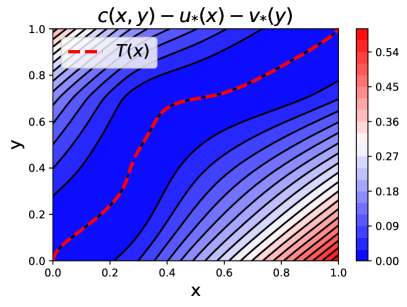
Figure 1: Left: dual constraint function $h(x,y)$ corresponding to the measures in Figures 2 and 2 in Appendix G. Note that $h$ attains its minimum on the graph of transportation map $T$, and is elsewhere positive. Right: changing parameterization flattens $h$ in the neighborhood of the graph of $T$. The red dotted line represent the zeros of both functions, and coincides with the graph of $T$ in the original parameterization (left).

Since $f$ is differentiable, by the properties of the Fenchel-Legendre conjugate it holds that $f^{\star}(\nabla f(z))=\nabla f(z)^{\top}z-f(z)$ for any $z\in X$ (Rockafellar, 1970). Therefore, from (i) we have that

$$\tilde{h}(x,z)=f(x)-f(z)-\nabla f(z)^{\top}(x-z).$$ (11)

Now, since $X$ is convex, we can characterize $f$ in terms of its Taylor expansion:

$$f(x)=f(z)+\nabla f(z)^{\top}(x-z)+(x-z)^{\top}\mathbf{R}(x,z)(x-z),\quad\forall x,z\in X,$$

where $\mathbf{R}$ is the integral reminder $\mathbf{R}(x,z)\operatorname{\overset{\operatorname{def}}{=}}\int_{0}^{1}(1-t)\mathbf{H}_{f}((1-t)x+tz)\mathrm{d}t$. This implies

$$\tilde{h}(x,z)=(x-z)^{\top}\mathbf{R}(x,z)(x-z),\quad\forall x,z\in X.$$ (12)

From (v), we get $\forall x,z,\mathbf{R}(x,z)\succeq\frac{\rho}{2}\operatorname{Id}$. In particular, for all $x,z\in X$, the matrix $\mathbf{R}(x,z)$ admits a positive square root $\sqrt{\mathbf{R}(x,z)}$. Further, since $\sqrt{\cdot}$ is $C^{\infty}$ on the closed set $\{\mathbf{A}\in\mathbb{S}_{+}(\mathbb{R}^{d}):\mathbf{A}\succeq\tfrac{\rho}{2}\operatorname{Id}\}$ and $\frac{\partial^{2}}{\partial x_{i}\partial x_{j}}f\in H^{s}(X)$ for all $i,j\in[d]$, the functions $r_{i,j}:(x,z)\mapsto e_{i}^{\top}\sqrt{\mathbf{R}(x,z)}e_{j}$ are in $H^{s}(X\times X)$ for all $i,j\in[d]$ (see Proposition 1 and Assumption 2b of Rudi et al., 2020), where $(e_{1},...,e_{d})$ is the canonical ONB of $\mathbb{R}^{d}$. Define now the functions

$$\tilde{w}_{i}(x,z)\operatorname{\overset{\operatorname{def}}{=}}\sum_{j=1}^{d}r_{i,j}(x,z)(e_{j}^{\top}(x-z)),\quad\forall x,z\in X,i\in[d].$$

From the above arguments, it holds that $\tilde{w}_{i}\in H^{s}(X\times X),i\in[d]$, and $\tilde{h}(x,z)=\sum_{i=1}^{d}\tilde{w}^{2}_{i}(x,z)$. Now, since $T$ is a $H^{s+1}$-diffeomorphism from $X$ to $Y$, changing parameterization again we have $h(x,y)=\sum_{i=1}^{d}w^{2}_{i}(x,y),~{}\forall(x,y)\in X\times Y$, with $w_{i}(x,y)=\tilde{w}_{i}(x,T^{-1}(y)),~{}\forall(x,y)\in X\times Y$.

We conclude by proving that $w_{i}\in H^{s}(X\times Y)$ for all $i\in[d]$. Indeed, from (iv) $T^{-1}$ is a $H^{s+1}$-diffeomorphism from $\bar{Y}$ to $\bar{X}$ and it is bi-Lipschitz (since $T$ and $T^{-1}$ are Lipschitz due to the continuity of their Hessian and the boundedness of $X,Y$). Define the map $Q$ as $(x,y)\mapsto(x,T^{-1}(y))$ and note that $Q\in H^{s+1}(X\times Y,\mathbb{R}^{2d})$, by construction. Note that $\tilde{w}_{i}\in H^{s}(X\times X)$ and has bounded weak derivatives of order $1$, since $s>d+1$ and $H^{s}(X\times X)$ is bounded (Adams and Fournier, 2003). The conditions above on $\tilde{w}_{i},Q$ guarantee that $w_{i}=\tilde{w}_{i}\circ Q$ belongs to $H^{s}(X\times Y)$ (see, e.g., Theorem 1.2 of Campbell et al., 2015).

Theorem 4.1 implies the existence of $A_{\star}\in\mathbb{S}_{+}({{{\mathcal{H}}_{XY}}})$ by effect of the reproducing property, when we consider a RKHS ${{\mathcal{H}}_{XY}}$ containing $H^{s}(X\times Y)$. The proof is in Appendix A, Appendix A.

Corollary 4.3.

Let ${{\mathcal{H}}_{XY}}$ be a RKHS such that $H^{s}(X\times Y)\subseteq{{\mathcal{H}}_{XY}}$. Under the hypothesis of Theorem 4.1, there exists a positive operator $A_{\star}\in\mathbb{S}_{+}({{{\mathcal{H}}_{XY}}})$ with rank at most $d$, such that

$$c(x,y)-u_{\star}(x)-v_{\star}(y)=\langle\phi(x,y),\,A_{*}\phi(x,y)\rangle_{{\mathcal{H}}_{XY}}.$$ (13)

Finally, the following corollary shows the effect of 1 on the existence of $A_{\star}$. Note indeed that such an assumption implies smoothness of the Kantorovich potentials (De Philippis and Figalli, 2014). If $m>d$ they are smooth enough to apply Theorem 4.1 and the corollary above. The proof of the following corollary is in Appendix A, Appendix A.

Corollary 4.4 (Effects of Asm. 1).

Let $\mu,\nu$ satisfy 1 for $m>d$. Let $(u_{\star},v_{\star})$ be Kantorovich potentials for $\mu,\nu$. Let ${{\mathcal{H}}_{X}}=H^{m+3}(X),{{\mathcal{H}}_{Y}}=H^{m+3}(Y),{{\mathcal{H}}_{XY}}=H^{m}(X\times Y)$. Then $u_{\star}\in{{\mathcal{H}}_{X}},v_{\star}\in{{\mathcal{H}}_{Y}}$ and there exists $A_{\star}\in\mathbb{S}_{+}({{{\mathcal{H}}_{XY}}})$ satifying Eq. 13 and $\operatorname{rank}A_{\star}\leq d$.

5 Subsampling the constraints

Given $\ell\in\mathbb{N}$ and a set of points $\tilde{Z}_{\ell}=\{(\tilde{x}_{1},\tilde{y}_{1}),\dots,(\tilde{x}_{\ell},\tilde{y}_{\ell})\}$, define the fill distance (Wendland, 2004),

$$h_{\ell}=\sup_{x\in X,y\in Y}\min_{j\in[\ell]}\|(x,y)-(\tilde{x}_{j},\tilde{y}_{j})\|.$$ (14)

The following theorem, that is an adaptation of Theorem 4 from Rudi et al. (2020), quantifies the error of subsampling the constraints in terms of the fill distance.

Theorem 5.1.

Let $X,Y$ satisfy 1a. Let $s\geq 3$ and $s>d$. Let ${{\mathcal{H}}_{X}}\subseteq H^{s}(X),{{\mathcal{H}}_{Y}}\subseteq H^{s}(Y),{{\mathcal{H}}_{XY}}=H^{s}(X\times Y)$. Let $\tilde{Z}_{\ell}\subset X\times Y$ be a set of points of cardinality $\ell$ and fill distance $h_{\ell}$ and let $u\in{{\mathcal{H}}_{X}},v\in{{\mathcal{H}}_{Y}},A\in\mathbb{S}_{+}({{{\mathcal{H}}_{XY}}})$ satisfy

$$c(\tilde{x}_{j},\tilde{y}_{j})-u(\tilde{x}_{j})-v(\tilde{y}_{j})=\langle\phi(\tilde{x}_{j},\tilde{y}_{j}),\,A\phi(\tilde{x}_{j},\tilde{y}_{j})\rangle_{{\mathcal{H}}_{XY}},\quad\forall j\in[\ell].$$ (15)

There exist $h_{0},C_{0}$ depending only on $s,d,X,Y$ such that, when $h_{\ell}\leq h_{0}$, then

$$c(x,y)\geq u(x)+v(y)-\varepsilon,~{}~{}~{}\forall x,y\in X\times Y,\quad\textrm{where}\quad\varepsilon=Qh^{s-d}_{\ell},$$

where $Q=C_{0}(\|u\|_{{\mathcal{H}}_{X}}+\|v\|_{{\mathcal{H}}_{Y}}+\mathrm{Tr}(A))$. Note that $h_{0},C_{0}$ depend only on $d,m,X,Y$.

The proof of the theorem above is reported in Appendix B, Appendix B. Using the theorem above we are able to show that, given a maximizer $(\hat{u},\hat{v},\hat{A})$ of Problem 3 the couple $(\hat{u}-\varepsilon/2,\hat{v}-\varepsilon/2)$ is admissible for Problem 1. This is a crucial step to bound $|\widehat{\text{OT}}-\text{OT}|$ in terms of the fill distance $h_{\ell}$ and it is stated next.

Theorem 5.2.

Let $\mu,\nu$ and $X,Y\subset\mathbb{R}^{d}$ satisfy 1a. Let $s>d$ and let ${{\mathcal{H}}_{X}},{{\mathcal{H}}_{Y}},{{\mathcal{H}}_{XY}}$ be RKHS on $X,Y,X\times Y$ such that ${{\mathcal{H}}_{X}}\subseteq H^{s}(X),{{\mathcal{H}}_{Y}}\subseteq H^{s}(Y),{{\mathcal{H}}_{XY}}=H^{s}(X\times Y)$. Assume that there exist two Kantorovich potentials $u_{\star},v_{\star}$ such that $u_{\star}\in{{\mathcal{H}}_{X}},v_{\star}\in{{\mathcal{H}}_{Y}}$ and there exists $A_{\star}\in\mathbb{S}_{+}({{{\mathcal{H}}_{XY}}})$ that satisfies Eq. 13. Let $\widehat{\text{OT}}$ be computed according to Eq. 6 using a set of $\ell\in\mathbb{N}$ points $\tilde{Z}_{\ell}\subset X\times Y$ with fill distance $h_{\ell}$. Let $h_{0},C_{0}$ as in Theorem 5.1. Let

$$\eta=C_{0}h^{s-d}_{\ell},\quad\gamma=\|w_{\mu}-\hat{w}_{\mu}\|_{{\mathcal{H}}_{X}}+\|w_{\nu}-\hat{w}_{\nu}\|_{{\mathcal{H}}_{Y}}.$$

When $h_{\ell}\leq h_{0}$, $\lambda_{2}>0$ and $\lambda_{1}$ is chosen such that $\lambda_{1}\geq 2\eta$, then

$$|\widehat{\text{OT}}-\text{OT}|~{}\leq~{}6\lambda_{1}\mathrm{Tr}(A_{\star})~{}+~{}6~{}\tfrac{(\gamma+\eta)^{2}}{\lambda_{2}}+6~{}\lambda_{2}~{}\big{(}\|u_{\star}\|^{2}_{{\mathcal{H}}_{X}}+\|v_{\star}\|^{2}_{{\mathcal{H}}_{Y}}).$$

The proof of the theorem above is in Appendix B, Appendix B. Theorem 5.2 together with Theorem 4.1 (in particular Corollary 4.4) allow to prove Theorem 2.1. To bound $h_{\ell}$ in terms of $\ell$, we used a result recalled in Lemma C.3.

Proof 5.3.

of Theorem 2.1. First note that $k_{X}=k_{m+1},k_{Y}=k_{m+1},k_{XY}=k_{m}$ imply that ${{\mathcal{H}}_{X}}=H^{m+1}(X),{{\mathcal{H}}_{Y}}=H^{m+1}(X),{{\mathcal{H}}_{XY}}=H^{m}(X\times Y)$. Then, by Corollary 4.4 we have that under 1 for any Kantorovich potentials $u_{\star},v_{\star}$ there exists a finite rank $A_{\star}\in\SS_{+}({{\mathcal{H}}_{XY}})$ such that $c(x,y)-u_{\star}(x)-v_{\star}(y)=\langle\phi(x,y),\,A_{*}\phi(x,y)\rangle_{{\mathcal{H}}_{XY}}$, and that $u_{\star}\in H^{m+3}(X)\subseteq H^{m+1}(X)={{\mathcal{H}}_{X}}$ and analogously $v_{\star}\in{{\mathcal{H}}_{Y}}$. Among them, we select the triplet minimizing $\|u_{\star}\|^{2}_{{{\mathcal{H}}_{X}}}+\|v_{\star}\|^{2}_{{{\mathcal{H}}_{Y}}}+\mathrm{Tr}(A_{\star})$ and we denote by $Q_{\mu,\nu}$ the resulting minimum. The proof is obtained by using this triplet in Theorem 5.2 and bounding $h_{\ell}$ as follows. First note that $X\times Y$ is a convex bounded set, since $X,Y$ have the same property. As recalled in Lemma C.1, Lemma C.1 of the appendix, convex bounded sets have the so-called uniform interior cone condition. This guarantees that $\ell$ i.i.d. points sampled from a distribution $\rho$, that has a density bounded away from zero, achieve the following bound on the fill distance: $h_{\ell}\leq(C\ell^{-1}\log(C^{\prime}\ell/\delta))^{-1/(2d)}$, with probability at least $1-\delta$, when $\ell\geq\ell_{0}$. Here $\ell_{0},C,C^{\prime}$ are constants that depend only on $d,X\times Y$ and the constant $c_{0}$ for which the density of $\rho$ is bounded away from zero. The final constants $C_{1},C_{2}$ depend also on $Q_{\mu,\nu}$.

We conclude with the following remark that is useful when we do not know the supports $X,Y$ or we are not able to sample i.i.d. points from the uniform distribution on them.

Remark 5.4 (Sampling from $X\times Y$ using $\mu\otimes\nu$).

Since, under 1, we have $\mu$ and $\nu$ bounded away from $0$, we can compute $\widehat{\text{OT}}$ by using $\ell$ i.i.d. samples from $\rho=\mu\otimes\nu$, obtaining the same guarantees as Theorem 2.1. Indeed, by inspecting the proof above, it is only required that $\rho$ has support $X\times Y$, and has a density that is bounded away from $0$. However, the constants $\ell_{0},C_{1},C_{2}$ will depend also on how far the density of $\rho$ is bounded away from $0$.

6 Estimators for the kernel mean embeddings of $\mu,\nu$

In this section we consider three classes of estimators $(\hat{w}_{\mu},\hat{w}_{\nu})$ for the kernel mean embeddings $w_{\mu}\in{{\mathcal{H}}_{X}}$ and $w_{\nu}\in{{\mathcal{H}}_{Y}}$ defined as $w_{\mu}=\int\phi_{X}(x)d\mu(x)$ and $w_{\nu}=\int\phi_{Y}(y)d\nu(y)$. As we observed in the introduction to Eq. 5, the operations we need to perform on $\hat{w}_{\mu},\hat{w}_{\nu}$ to compute the algorithm are the evaluation of the norm $\|\hat{w}_{\mu}\|^{2}_{{\mathcal{H}}_{X}}$ and the evaluation of $\hat{w}_{\mu}(\tilde{x}_{i})$ for $i\in[\ell]$ (and the same for $\hat{w}_{\nu}$). For each class we will specify such operations. Here, we assume that $\phi_{X},\phi_{Y}$ are uniformly bounded maps (as for the Sobolev kernel, where $\sup_{x\in X}\|\phi_{X}(x)\|^{2}_{{\mathcal{H}}_{X}}=\sup_{x\in X}k(x,x)=1$, see Proposition 3.1). Clearly a class of estimators must only be chosen if we are able to perform the required operations.

Exact integral.

Here we take $\hat{w}_{\mu}:=w_{\mu}$ and $\hat{w}_{\nu}=w_{\nu}$ and we report only the operations for $\mu$ since the ones for $\nu$ are the same. This is the estimator that leads to the best rates as shown in Theorem 1.1 and Corollary 2.2. However it requires to perform the most difficult operations, i.e., (1) $\hat{w}_{\mu}(\tilde{x}_{i})=\langle w_{\mu},\,\phi_{X}(\tilde{x}_{i})\rangle_{{\mathcal{H}}_{X}}=\int_{X}\langle\phi_{X}(\tilde{x}_{i}),\,\phi_{X}(x)\rangle d\mu(x)=\int_{X}k_{X}(\tilde{x}_{i},x)d\mu(x)$ for all $i\in[\ell]$; (2) $\|\hat{w}_{\mu}\|^{2}_{{\mathcal{H}}_{X}}=\langle w_{\mu},\,w_{\mu}\rangle_{{\mathcal{H}}_{X}}=\int_{X}\langle\phi_{X}(x),\,\phi_{X}(x^{\prime})\rangle_{{\mathcal{H}}_{X}}d\mu(x)d\mu(x^{\prime})=\int_{X}k_{X}(x,x^{\prime})d\mu(x)d\mu(x^{\prime})$. Moreover the costs $C,E$ in Eq. 7 are $C=O(1),E=O(1)$.

Evaluation estimator.

Here we assume we are able to evaluate $\mu(x_{j})$ in a given set of points $x_{1},\dots,x_{n_{\mu}}$ with $n_{\mu}\in\mathbb{N}$ (analogously for $\nu$ on $y_{1},\dots,y_{n_{\nu}}$ with $n_{\nu}\in\mathbb{N}$). We define the estimators as $\hat{w}_{\mu}=\int_{X}\phi_{X}(x)\hat{g}_{\mu}(x)dx$ (analogously for $\hat{w}_{\nu}$). Here $\hat{g}_{\mu}\in{{\mathcal{H}}_{X}}$ is the kernel least squares estimator (Narcowich et al., 2005) of the density $\mu$ defined as $\hat{g}_{\mu}(x)=\sum_{j\in[n_{\mu}]}\alpha_{j}k_{X}(x_{j},x)$ where $\alpha={\bf K}_{X}^{-1}c_{\mu}$ and ${\bf K}_{X}\in\mathbb{R}^{n_{\mu}\times n_{\mu}}$, $({\bf K}_{X})_{i,j}=k_{X}(x_{i},x_{j})$ for all $i,j\in[n_{\mu}]$, while $c_{\mu}\in\mathbb{R}^{n_{\mu}}$, $c_{\mu}=(\mu(x_{1}),\dots,\mu(x_{n}))$. In this case the steps are: (1) $\hat{w}_{\mu}(\tilde{x}_{i})=\int_{X}\langle\phi_{X}(\tilde{x}_{i}),\,\phi_{X}(x)\rangle\hat{g}_{\mu}(x)dx=\sum_{j\in[n_{\mu}]}\alpha_{j}\int_{X}k_{X}(\tilde{x}_{i},x)k_{X}(x_{j},x)dx,i\in[\ell]$, and (2) $\|\hat{w}_{\mu}\|^{2}_{{\mathcal{H}}_{X}}=\sum_{i,t\in[n_{\mu}]}\alpha_{i}\alpha_{t}\int_{X}\int_{X}k_{X}(x_{i},x)k(x,x^{\prime})k(x_{t},x^{\prime})dxdx^{\prime}$. Moreover the costs $C,E$ in Eq. 7 are $C=O(n_{\mu}^{3}+n_{\nu}^{3}),E=O(n_{\mu}+n_{\nu})$.

Sample estimator.

Here we assume we are able to sample from $\mu,\nu$. Let $x_{1},\dots,x_{n_{\mu}}$, $n_{\mu}\in\mathbb{N}$, be sampled i.i.d. from $\mu$ and $y_{1},\dots,y_{n_{\nu}}$, $n_{\nu}\in\mathbb{N}$ be sampled i.i.d. from $\nu$. The estimators are $\hat{w}_{\mu}=\frac{1}{n_{\mu}}\sum_{j\in[n_{\mu}]}\phi_{X}(x_{j})$, and analogously for $\hat{w}_{\nu}$. In this case the operations are: (1) $\hat{w}_{\mu}(\tilde{x}_{i})=\frac{1}{n_{\mu}}\sum_{j\in[n_{\mu}]}k_{X}(x_{j},\tilde{x}_{i})$, and (2) $\|\hat{w}_{\mu}\|^{2}_{{\mathcal{H}}_{X}}=\frac{1}{n_{\mu}^{2}}\sum_{i,j\in[n_{\mu}]}k_{X}(x_{i},x_{j})$. Moreover the costs $C,E$ in Eq. 7 are $C=O(n_{\mu}^{2}+n_{\nu}^{2}),E=O(n_{\mu}+n_{\nu})$.

The effects of the estimators above are studied in Theorem 1.1 and Corollary 2.2, reported in Section 1 and proven in Appendix E, Appendix E, using standard tools from approximation theory and machine learning with kernel methods (Wendland, 2004; Caponnetto and De Vito, 2007; Muandet et al., 2017).

Acknowledgements.

This work was funded in part by the French government under management of Agence Nationale de la Recherche as part of the “Investissements d’avenir” program, reference ANR-19-P3IA-0001 (PRAIRIE 3IA Institute). We also acknowledge support from the European Research Council (grants SEQUOIA 724063 and REAL 947908), and Région Ile-de-France.

Appendix A Proofs of Corollary 4.3 and Corollary 4.4

Proof A.1.

of Corollary 4.3. Define $h(x,y):=c(x,y)-u_{\star}(x)-v_{\star}(y),\forall(x,y)\in X\times Y$. By Theorem 4.1, there exist $w_{1},...,w_{d}\in H^{s}(X\times Y)$ such that $h=\sum_{i=1}^{d}w_{i}^{2}$. Since $H^{s}(X\times Y)\subseteq{{\mathcal{H}}_{XY}}$, then $w_{1},\dots,w_{d}\in{{\mathcal{H}}_{XY}}$. Hence $A_{\star}=\sum_{i=1}^{d}w_{i}\otimes w_{i}\in\mathbb{S}_{+}({{{\mathcal{H}}_{XY}}})$. Moreover, by the reproducing property of ${{\mathcal{H}}_{XY}}$, $A_{\star}$ satisfies $\langle\phi(x,y),\,A_{\star}\phi(x,y)\rangle_{{\mathcal{H}}_{XY}}=\sum_{i=1}^{d}\langle w_{j},\,\phi(x,y)\rangle_{{\mathcal{H}}_{XY}}^{2}=\sum_{i=1}^{d}w(x,y)^{2}=h(x,y)$, for all $(x,y)\in X\times Y$. Finally, note that $\operatorname{rank}A_{\star}\leq d$ by construction.

Proof A.2.

of Corollary 4.4. Theorem 3.3 in De Philippis and Figalli (2014) implies that Kantorovich potentials satisfy $u_{\star}\in C^{m+2,1}(\overline{X}),v_{\star}\in C^{m+2,1}(\overline{Y})$, where $C^{m+2,1}(\overline{Z})$ for an open set $Z$ is the space of real functions over $Z$ that are $m+2$-times differentiable, with all the derivatives of order $m+2$ that are Lipschitz continuous (Adams and Fournier, 2003, 1.29, Page 10). Since $X$ is convex and bounded, then Lipschitz continuity of all the derivatives of order $m+2$ implies that all the weak derivatives up to order $m+3$ are in $L^{\infty}(X)$. Since $L^{\infty}(X)\subset L^{2}(X)$, by the boundedness of $X$, we have $C^{m+2,1}(\overline{X})\subset H^{m+3}_{2}(X)$. Analogously $C^{m+2,1}(\overline{Y})\subset H^{m+3}_{2}(Y)$. Then $u_{\star}\in H^{m+3}(X),v_{\star}\in H^{m+3}(Y)$, and we can apply Theorem 4.1 and Corollary 4.3 with $s=m+1$, when $m>d$, which guarantee the existence of $A_{\star}\in\mathbb{S}_{+}({{{\mathcal{H}}_{XY}}})$, since ${{\mathcal{H}}_{XY}}=H^{s}(X\times Y)$.

Appendix B Proofs of Theorem 5.1 and Theorem 5.2

Proof B.1.

of Theorem 5.1. Let $f(x,y)=c(x,y)-u(x){\bf 1}_{X}(y)-v(y){\bf 1}_{Y}(x)-\langle\phi(x,y),\,A\phi(x,y)\rangle$ for any $x,y\in X\times Y$, where the function ${\bf 1}_{X}(x)$ and ${\bf 1}_{Y}(y)$ are respectively the constant function $1$ over $X$ and over $Y$. By construction $f\in H^{s}(X\times Y)$. Since $X,Y$ are open bounded convex sets, then $X\times Y$ has the same property which, in turn, implies the so-called uniform interior cone condition (see Lemma C.1, Lemma C.1 in the appendix). Then we can apply Theorem 1 of Narcowich et al. (2005) for which there exist $h_{0},C_{0}$ depending only on $s,d,X,Y$ such that for any $h_{\ell}\leq h_{0}$ the following holds

$$\sup_{(x,y)\in X\times Y}|f(x,y)|\leq\varepsilon,\quad\varepsilon:=C_{1}h_{\ell}^{s-d}|f|_{H^{s}(X\times Y)},$$

where $|g|_{H^{s}(X\times Y)}:=\sum_{|\alpha|=s}\|D^{\alpha}g\|_{L^{2}(X\times Y)}\leq\|g\|_{H^{s}(X\times Y)}$ for any $g\in H^{s}(X\times Y)$. Let $r_{A}(x,y)=\langle\phi(\tilde{x}_{j},\tilde{y}_{j}),\,A\phi(\tilde{x}_{j},\tilde{y}_{j})\rangle_{{\mathcal{H}}_{XY}}$, we have

$$|f|_{H^{s}(X\times Y)}\leq|c|_{H^{s}(X\times Y)}+|u{\bf 1}_{X}|_{H^{s}(X\times Y)}+|v{\bf 1}_{Y}|_{H^{s}(X\times Y)}+|r_{A}|_{H^{s}(X\times Y)}.$$

Now $|c|_{H^{s}(X\times Y)}=0$ since $c$ is the quadratic cost and $s\geq 3$ and $|u{\bf 1}_{X}|_{H^{s}(X\times Y)}=|u|_{H^{s}(X)}\leq\|u\|_{H^{s}(X)}$, $|v{\bf 1}_{Y}|_{H^{s}(X\times Y)}=|v|_{H^{s}(Y)}\leq\|v\|_{H^{s}(Y)}$. We recall now that for any two Banach spaces satisfying $B\subseteq A$, we have $\|w\|_{A}\leq\|w\|_{B}$ for any $w\in B$. Then $\|u\|_{H^{s}(X)}\leq\|u\|_{{{\mathcal{H}}_{X}}}$, $\|v\|_{H^{s}(Y)}\leq\|v\|_{{{\mathcal{H}}_{Y}}}$. Finally $|r_{A}|_{H^{s}(X\times Y)}\leq\|r_{A}\|_{H^{s}(X\times Y)}\leq C_{1}\mathrm{Tr}(A)$ via Lemma 9 page 41 from Rudi et al. (2020) and Proposition 1 of the same paper, where $C_{2}$ depends only on $s,X,Y$. Now since $|f(x,y)|\leq\varepsilon$ for all $(x,y)\in X\times Y$, and since $r_{A}(x,y)\geq 0$ for any $x,y\in X\times Y$ since $A$ is a positive operator, we have

$$-\varepsilon\leq f(x,y)\leq f(x,y)+r_{A}(x,y)=c(x,y)-u(x)-v(y),\quad\forall(x,y)\in X\times Y.$$

The final result is obtained by defining $C_{0}=C_{1}(1+C_{2})$.

Proof B.2.

of Theorem 5.2. Denote by $V(u,v)$ the functional of Problem 1 and by $\hat{V}_{\lambda_{1},\lambda_{2}}(u,v,A)$ the functional of Problem 3. Then $\text{OT}=V(u_{\star},v_{\star})$. Denote by $\Delta(u,v)$ the quantity

$$\Delta(u,v)=|\langle u,\,\hat{w}_{\mu}-w_{\mu}\rangle_{{\mathcal{H}}_{X}}+\langle v,\,\hat{w}_{\nu}-w_{\nu}\rangle_{{\mathcal{H}}_{Y}}|.$$

Denote by $\hat{R}^{2}(u,v)$ the quantity $\hat{R}^{2}(u,v)=\|u\|^{2}_{{\mathcal{H}}_{X}}+\|v\|^{2}_{{\mathcal{H}}_{Y}}$ for any $u\in{{\mathcal{H}}_{X}},v\in{{\mathcal{H}}_{Y}}$.

Step 0. Admissibility of $u_{\star},v_{\star},A_{\star}$ and existence of a maximizer.

Note that $(u_{\star},v_{\star},A_{\star})$ is an admissible point for Problem 3, since the triple satisfies $c_{\star}(x,y)-u_{\star}(x)-v_{\star}(y)=\langle\phi(x,y),\,A_{\star}\phi(x,y)\rangle~{}\forall(x,y)\in X\times Y$, and Problem 3 applies the same constraints but on a subset of $X\times Y$. Moreover $\lambda_{1},\lambda_{2}>0$, this is enough to guarantee the existence of a maximizer for Problem 3. Indeed, as we recall in Lemma D.3, Lemma D.3, in the appendix, a form of representer theorem holds for Problem 3 (see Lemma D.1, Lemma D.1 in the appendix), moreover the functional is coercive on the finite-dimensional space induced by the data, it has an upper bound and the problem has an admissible point. Now denote by $(\hat{u},\hat{v},\hat{A})$ a maximizer of Problem 3 and define $\overline{\text{OT}}:=\hat{V}_{\lambda_{1},\lambda_{2}}(\hat{u},\hat{v},\hat{A})$. By construction $\overline{\text{OT}}$ is the maximum of $\hat{V}_{\lambda_{1},\lambda_{2}}$. Then by definition of $\widehat{\text{OT}}$ in Eq. 6,

$$\widehat{\text{OT}}=\overline{\text{OT}}+\lambda_{1}\mathrm{Tr}(\hat{A})+\lambda_{2}R^{2}(\hat{u},\hat{v}).$$

Step 1. Subsampling the inequality.

The assumption on $h_{\ell}$ and the fact that the constraints of Eq. 3 satisfy Eq. 15 allow to apply Theorem 5.1, from which there exists a couple $(\hat{u}_{\varepsilon},\hat{v}_{\varepsilon})$ that is admissible for Problem 1, where $\hat{u}_{\varepsilon}=\hat{u}-\frac{\varepsilon}{2}$ and $\hat{v}_{\varepsilon}=\hat{v}-\frac{\varepsilon}{2}$, for any $\varepsilon\geq C_{0}h^{s-d}_{\ell}(\|\hat{u}\|_{{\mathcal{H}}_{X}}+\|\hat{v}\|_{{\mathcal{H}}_{Y}}+\mathrm{Tr}(\hat{A}))$. In particular, since $\|u\|_{{\mathcal{H}}_{X}}+\|v\|_{{\mathcal{H}}_{Y}}\leq 2R(\hat{u},\hat{v})$, we choose $\varepsilon=\eta(R(\hat{u},\hat{v})+\mathrm{Tr}(\hat{A}))$, with $\eta=C_{0}h^{s-d}_{\ell}$.

Step 2. Bounding $\widehat{\text{OT}}-\text{OT}$.

Since OT is the maximum of Problem 1 then

$$\text{OT}=V(u_{\star},v_{\star}) \geq V(\hat{u}_{\varepsilon},\hat{v}_{\varepsilon})=V(\hat{u},\hat{v})-\varepsilon\geq\widehat{\text{OT}}-\Delta(\hat{u},\hat{v})-\varepsilon.$$ (16)

Analogously, since $(\hat{u},\hat{v},\hat{A})$ maximize Problem 3, then

$$\overline{\text{OT}}=\hat{V}_{\lambda_{1},\lambda_{2}}(\hat{u},\hat{v},\hat{A}) \geq\hat{V}_{\lambda_{1},\lambda_{2}}(u_{\star},v_{\star},A_{\star})$$ (17)

$$=V(u_{\star},v_{\star})-\left[V(u_{\star},v_{\star})-\hat{V}_{\lambda_{1},\lambda_{2}}(u_{\star},v_{\star},A_{\star})\right]$$ (18)

$$\geq\text{OT}-\Delta(u_{\star},v_{\star})-\lambda_{1}\mathrm{Tr}(A_{\star})+\lambda_{2}R^{2}(u_{\star},v_{\star}).$$ (19)

By expressing $\overline{\text{OT}}$ in terms of $\widehat{\text{OT}}$ in the inequality above and combining it with Eq. 16, we have

$$\lambda_{1}\mathrm{Tr}(\hat{A}-A_{\star})+\lambda_{2}(R^{2}(\hat{u},\hat{v})-R^{2}(u_{\star},v_{\star}))-\Delta(u_{\star},v_{\star})\leq\widehat{\text{OT}}-\text{OT}\leq\Delta(\hat{u},\hat{v})+\varepsilon.$$ (20)

Step 3. Bound on $\Delta$.

Note that for two RKHS ${\mathcal{H}},{\mathcal{K}}$ and any $u,v\in{\mathcal{H}},w,z\in{\mathcal{K}}$, the following identity holds: $\langle u,\,v\rangle_{\mathcal{H}}+\langle w,\,z\rangle_{\mathcal{K}}=\langle(u,w),\,(v,z)\rangle_{{\mathcal{H}}\oplus{\mathcal{K}}}$, where ${\mathcal{H}}\oplus{\mathcal{K}}$ is a RKHS (Aronszajn, 1950). This implies $(\langle u,\,v\rangle_{\mathcal{H}}+\langle w,\,z\rangle_{\mathcal{K}})^{2}=\|(u,w)\|_{{\mathcal{H}}\oplus{\mathcal{K}}}^{2}\|(v,z)\|_{{\mathcal{H}}\oplus{\mathcal{K}}}^{2}=(\|u\|^{2}_{\mathcal{H}}+\|v\|^{2}_{\mathcal{K}})(\|w\|^{2}_{\mathcal{H}}+\|z\|^{2}_{\mathcal{K}})$. Applying this inequality to $\Delta$ leads to the following result:

$$\Delta(a,b)\leq R(a,b)\gamma.$$ (21)

Step 4. Bounding $\mathrm{Tr}(\hat{A}),R(\hat{u},\hat{v})$.

The bound Eq. 20 implies

$$\lambda_{1}\mathrm{Tr}(\hat{A})+\lambda_{2}R^{2}(\hat{u},\hat{v})\leq\lambda_{1}\mathrm{Tr}(A_{\star})+\lambda_{2}R^{2}(u_{\star},v_{\star})+\Delta(u_{\star},v_{\star})+\Delta(\hat{u},\hat{v})+\varepsilon.$$ (22)

By bounding $\Delta$ via Eq. 21, expanding the definition of $\varepsilon$ and reordering the terms in the inequality above, we obtain

$$\alpha\mathrm{Tr}(\hat{A})+\lambda_{2}R^{2}(\hat{u},\hat{v})-\beta R(\hat{u},\hat{v})\leq\lambda_{1}\mathrm{Tr}(A_{\star})+\lambda_{2}R^{2}(u_{\star},v_{\star})+\gamma R(u_{\star},v_{\star}),$$ (23)

with $\alpha=\lambda_{1}-\eta$ and $\beta=\gamma+\eta$. By completing the square in $R^{2}(\hat{u},\hat{v})$, the inequality above is rewritten as

$$\alpha\mathrm{Tr}(\hat{A})+\lambda_{2}(R(\hat{u},\hat{v})-\tfrac{\beta}{2\lambda_{2}})^{2}\leq\lambda_{1}\mathrm{Tr}(A_{\star})+\lambda_{2}R^{2}(u_{\star},v_{\star})+\gamma R(u_{\star},v_{\star})+\tfrac{\beta^{2}}{4\lambda_{2}}.$$ (24)

Since $\alpha\geq\lambda_{1}/2$, by the assumption $\lambda_{1}\geq 2\eta$, the inequality above implies

$$\tfrac{\lambda_{1}}{2}\mathrm{Tr}(\hat{A})\leq\lambda_{2}S,\quad R(\hat{u},\hat{v})\leq\tfrac{\beta}{2\lambda_{2}}+\sqrt{S}.$$ (25)

with $S:=\tfrac{\lambda_{1}}{\lambda_{2}}\mathrm{Tr}(A_{\star})+R^{2}(u_{\star},v_{\star})+\tfrac{\gamma}{\lambda_{2}}R(u_{\star},v_{\star})+\tfrac{\beta^{2}}{4\lambda_{2}^{2}}.$

Conclusion.

From the lower bound in Eq. 20 and the bound Eq. 21 on $\Delta$, we have that

$$\widehat{\text{OT}}-\text{OT}\geq-\lambda_{1}\mathrm{Tr}(A_{\star})-\lambda_{2}R^{2}(u_{\star},v_{\star})-\gamma R(u_{\star},v_{\star})\geq-\lambda_{2}S.$$

From the upper bound in Eq. 20, the bound for $\Delta$ in Eq. 21, the bound for $\mathrm{Tr}(\hat{A}),R(\hat{u},\hat{v})$ in Eq. 25, the definition of $\varepsilon$, and the fact that $\lambda_{1}\geq 2\eta$, we have

$$\widehat{\text{OT}}-\text{OT} \leq\beta R(\hat{u},\hat{v})+\tfrac{\lambda_{1}}{2}\mathrm{Tr}(\hat{A})\leq\tfrac{\beta^{2}}{2\lambda_{2}}+\beta\sqrt{S}+\lambda_{2}S.$$ (26)

Then $|\widehat{\text{OT}}-\text{OT}|\leq\tfrac{\beta^{2}}{2\lambda_{2}}+\beta\sqrt{S}+\lambda_{2}S.$ To conclude, by noting that $S\leq\tfrac{\lambda_{1}}{\lambda_{2}}\mathrm{Tr}(A_{\star})+(R(u_{\star},v_{\star})+\tfrac{\beta}{2\lambda_{2}^{2}})^{2}$, since $\gamma\leq\beta$, and that $(a+b+c)^{2}\leq 3a^{2}+3b^{2}+3c^{2}$ for any $a,b,c\geq 0$, we have

$$\tfrac{\beta^{2}}{2\lambda_{2}}+\beta\sqrt{S}+\lambda_{2}S \leq 2\lambda_{2}(\tfrac{\beta}{2\lambda}+\sqrt{S})^{2}\leq 2\lambda_{2}\left(R(u_{\star},v_{\star})+\tfrac{\beta}{\lambda_{2}}+\sqrt{\tfrac{\lambda_{1}}{\lambda_{2}}\mathrm{Tr}(A_{\star})}\right)^{2}$$ (27)

$$\leq 6\lambda_{2}(R^{2}(u_{\star},v_{\star})+\tfrac{\beta^{2}}{\lambda_{2}^{2}}+\tfrac{\lambda_{1}}{\lambda_{2}}\mathrm{Tr}(A_{\star})).$$ (28)

Appendix C Additional results on convex sets and random points

We first recall that the following property about bounded sets in Euclidean spaces.

Lemma C.1 (Krieg and Sonnleitner (2020)).

Let $Z\subset\mathbb{R}^{q}$, $q\in\mathbb{N}$ be a non-empty open set. The following holds:

1. If $Z$ is a bounded Lipschitz domain (Grisvard, 1985), then it satisfies the uniform interior cone condition (Wendland, 2004).

2. If $Z$ is a convex bounded set, then it is a bounded Lipschitz domain.

Proof C.2.

For the first point, see Lemma 5 of Krieg and Sonnleitner (2020) or Theorem 1.2.2.2 of Grisvard (1985). For the second point, see Lemma 4 of Krieg and Sonnleitner (2020) or Lemma 7 in Dekel and Leviatan (2004). Also, the fact that a convex bounded open set has the uniform interior cone condition is implied by Proposition 11.26 of Wendland (2004), that proves it for the more general class of sets called star shaped sets w.r.t. a ball.

Lemma C.3 (Fill distance of i.i.d points on a u.i.c. set (Reznikov and Saff, 2016)).

Let $Z\subset\mathbb{R}^{q}$, $q\in\mathbb{N}$ be a non-empty open set satisfying the uniform interior cone condition (see Lemma C.1). Let $\tilde{Z}_{\ell}$ be a collection of $\ell$ points sampled independently and uniformly at random from a probability $\rho$ that admits density (denote it by $p$) and such that $p(z)\geq c_{0}>0$ for any $z\in Z$. Let $\delta\in(0,1]$. Then there exist $\ell_{0},C_{1},C_{2}$ depending on $c_{0},Z,\rho,q,r_{0}$ such that for $\ell\geq\ell_{0}$, the following holds with probability at least $1-\delta$:

$$h_{\ell}\leq(C_{1}\ell^{-1}\log(C_{2}\ell/\delta))^{1/q}.$$

Proof C.4.

The uniform interior cone condition guarantees that there exists a cone $C$ such that for any $z\in Z$ there exists a spherical cone of radius $r$ such that $C_{z}\subseteq Z$ that is congruent to $C$ and with vertex in $z$. Then, for any $r\leq r_{0}$ there exists $c_{1}$ such that

$$\rho(B(z,r)\cap Z)\geq\rho(B(z,r)\cap C_{z})\geq c_{0}\frac{\textrm{vol}(B(z,r)\cap C_{z})}{\textrm{vol}(Z)}\geq\frac{c_{0}c_{1}}{\textrm{vol}(Z)}r^{q}.$$

Then we can apply Theorem 2.1 of Reznikov and Saff (2016) with $\Phi(r)=\frac{c_{0}c_{1}}{\textrm{vol}(Z)}r^{q}$ obtaining that there exists $\ell_{0},C_{1},C_{2}$ depending on $c_{0},c_{1},q,r_{0},Z$ such that with probability at least $1-\delta$,

$$h_{\ell}\leq(C_{1}\ell^{-1}\log(C_{2}\ell/\delta))^{1/q}.$$

Appendix D Representer theorem and coercivity for Problem (3)

We first adapt the proof of the representer theorem from Marteau-Ferey et al. (2020). We use it to prove coercivity of the functional. Given the RKHS ${{\mathcal{H}}_{X}},{{\mathcal{H}}_{Y}},{{\mathcal{H}}_{XY}}$ and with the same notation of Problem (3) define $\hat{{\mathcal{H}}}_{X}=\textrm{span}\{\hat{w}_{\mu},\phi_{X}(\tilde{x}_{1}),\dots,\phi_{X}(\tilde{x}_{\ell})\}$, $\hat{{\mathcal{H}}}_{Y}=\textrm{span}\{\hat{w}_{\nu},\phi_{Y}(\tilde{y}_{1}),\dots,\phi_{Y}(\tilde{y}_{\ell})\}$ and $\hat{{\mathcal{H}}}_{XY}=\textrm{span}\{\phi(x_{1},y_{1}),\dots,\phi(x_{\ell},y_{\ell})\}$.

Lemma D.1 (Representer theorem, Marteau-Ferey et al. (2020)).

Let $\lambda_{1},\lambda_{2}>0$. Denote by $V_{\lambda_{1},\lambda_{2}}(u,v,A)$ the objective function of Problem (3). Let $u_{1}\in\hat{{\mathcal{H}}}_{X},u_{2}\in\hat{{\mathcal{H}}}_{X}^{\bot}$, $v_{1}\in\hat{{\mathcal{H}}}_{Y},v_{2}\in\hat{{\mathcal{H}}}_{Y}^{\bot}$ and $A_{1}\in\hat{{\mathcal{H}}}_{XY}\otimes\hat{{\mathcal{H}}}_{XY},A_{2}\in\hat{{\mathcal{H}}}_{XY}^{\bot}\otimes\hat{{\mathcal{H}}}_{XY},A_{3}\in\hat{{\mathcal{H}}}_{XY}^{\bot}\otimes\hat{{\mathcal{H}}}_{XY}^{\bot}$. Assume that $u_{2}$ or $v_{2}$ or $A_{2}$ or $A_{3}$ are different from $0$. Set $u=u_{1}+u_{2}$, $v=v_{1}+v_{2}$ and $A=A_{1}+A_{2}+A_{2}^{*}+A_{3}$ and assume that $u,v,A$ is an admissible point for Problem (3) Then

1. $(u_{1},v_{1},A_{1})$ is an admissible point for Problem (3),

2. $V_{\lambda_{1},\lambda_{2}}(u_{1},v_{1},A_{1})>V_{\lambda_{1},\lambda_{2}}(u,v,A)$.

Proof D.2.

We can decompose any $u\in{{\mathcal{H}}_{X}},v\in{{\mathcal{H}}_{Y}},A\in\mathbb{S}_{+}({{{\mathcal{H}}_{XY}}})$ as $u_{1}\in\hat{{\mathcal{H}}}_{X},u_{2}\in\hat{{\mathcal{H}}}_{X}^{\bot}$, $v_{1}\in\hat{{\mathcal{H}}}_{Y},v_{2}\in\hat{{\mathcal{H}}}_{Y}^{\bot}$ and $A_{1}\in\hat{{\mathcal{H}}}_{XY}\otimes\hat{{\mathcal{H}}}_{XY},A_{2}\in\hat{{\mathcal{H}}}_{XY}^{\bot}\otimes\hat{{\mathcal{H}}}_{XY},A_{3}\in\hat{{\mathcal{H}}}_{XY}^{\bot}\otimes\hat{{\mathcal{H}}}_{XY}^{\bot}$. Note that the components $u_{2},v_{2},A_{2},A_{3}$ do not impact the constraints or the functional but are only penalized by the regularizer, indeed $\langle u_{2},\,\phi_{X}(\tilde{x}_{i})\rangle_{{\mathcal{H}}_{X}}=0$ since $\phi_{X}(\tilde{x}_{i})\in\hat{{\mathcal{H}}}_{X}$, while $u_{2}\in\hat{{\mathcal{H}}}_{X}^{\bot}$, then

$$u(\tilde{x_{i}})=\langle u,\,\phi_{X}(\tilde{x}_{i})\rangle_{{\mathcal{H}}_{X}}=\langle u_{1},\,\phi_{X}(\tilde{x}_{i})\rangle_{{\mathcal{H}}_{X}}+\langle u_{2},\,\phi_{X}(\tilde{x}_{i})\rangle_{{\mathcal{H}}_{X}}=\langle u_{1},\,\phi_{X}(\tilde{x}_{i})\rangle_{{\mathcal{H}}_{X}}=u_{1}(\tilde{x}_{i}).$$

The same reasoning holds for $v(\tilde{x}_{i})$ and for $\langle u,\,w_{\mu}\rangle_{{\mathcal{H}}_{X}},\langle v,\,w_{\nu}\rangle_{{\mathcal{H}}_{Y}}$. For $A$ analogously we have that $t=A_{2}\phi(\tilde{x}_{i},\tilde{y}_{i})\in\hat{{\mathcal{H}}}_{XY}^{\bot}$ so $\langle\phi(\tilde{x}_{i},\tilde{y}_{i}),\,A_{2}\phi(\tilde{x}_{i},\tilde{y}_{i})\rangle_{{\mathcal{H}}_{XY}}=\langle\phi(\tilde{x}_{i},\tilde{y}_{i}),\,t\rangle_{{\mathcal{H}}_{XY}}=0$ and similarly for $A_{3}$, we have $\langle\phi(\tilde{x}_{i},\tilde{y}_{i}),\,A_{3}\phi(\tilde{x}_{i},\tilde{y}_{i})\rangle_{{\mathcal{H}}_{XY}}=0$. Let’s see what happens to the penalization terms. For the quadratic term, we have $-\|u\|^{2}_{{\mathcal{H}}_{X}}=-\|u_{1}\|^{2}_{{\mathcal{H}}_{X}}-\|u_{2}\|^{2}_{{\mathcal{H}}_{X}}<-\|u_{1}\|^{2}_{{\mathcal{H}}_{X}}$ and analogously for $v$. For the trace term we have $\mathrm{Tr}(A)=\mathrm{Tr}(A_{1})+\mathrm{Tr}(A_{3})$. Moreover $A\in\mathbb{S}_{+}({{{\mathcal{H}}_{XY}}})$ implies that $A_{1}\succeq 0$ and by the Schur complement property $A_{3}\succeq A_{2}^{*}A_{1}^{-1}A_{2}\succeq 0$. Then if $A_{3}\succeq 0$ and different from zero we have $-\mathrm{Tr}(A)<-\mathrm{Tr}(A_{1})$. If $A_{2}$ is different from zero this implies by the Schur complement property that $A_{3}$ is a positive definite operator different from zero and so $-\mathrm{Tr}(A)<-\mathrm{Tr}(A_{1})$.

Lemma D.3 (Problem (3) has a maximizer).

When $\lambda_{1},\lambda_{2}>0$ and when there exists an admissible point $(\bar{u},\bar{v},\bar{A})$ with $\bar{u}\in{{\mathcal{H}}_{X}},\bar{v}\in{{\mathcal{H}}_{Y}},\bar{A}\in\mathbb{S}_{+}({{{\mathcal{H}}_{XY}}})$, Problem (3) admits a maximizer.

Proof D.4.

First define $S={{\mathcal{H}}_{X}}\times{{\mathcal{H}}_{Y}}\times({{\mathcal{H}}_{XY}}\otimes{{\mathcal{H}}_{XY}})$ and $\hat{S}=\hat{{\mathcal{H}}}_{X}\times\hat{{\mathcal{H}}}_{Y}\times(\hat{{\mathcal{H}}}_{XY}\otimes\hat{{\mathcal{H}}}_{XY})$. From the lemma above, we have that for any admissible point in $S\setminus\hat{S}$ there exists another admissible point in $\hat{S}$ that has a strictly larger value. Note moreover that $\hat{S}$ is a finite dimensional Hilbert space (with dimension at most $\ell^{2}(\ell+1)^{2}$) and that (minus) the functional of Problem (3) is coercive on it. Note moreover that Eq. 3 is bounded from above since $V_{\lambda_{1},\lambda_{2}}(u,v,A)\leq\|u\|_{{\mathcal{H}}_{X}}\|\hat{w}_{\mu}\|_{{\mathcal{H}}_{X}}+\|v\|_{{\mathcal{H}}_{Y}}\|\hat{w}_{\nu}\|_{{\mathcal{H}}_{Y}}-\lambda_{2}(\|u\|^{2}_{{\mathcal{H}}_{X}}+\|v\|^{2}_{{\mathcal{H}}_{Y}})$ has a maximum in $u,v$. Since Problem (3) has also an admissible point by assumption, then it admits at least one maximizer (see, e.g., Proposition 3.2.1, Page 119 of Bertsekas, 2009).

Appendix E Proof of Corollary 2.2 and Theorem 1.1

Proof E.1.

of Corollary 2.2. The result is obtained by plugging in Theorem 2.1 the bounds on $\gamma=\|w_{\mu}-\hat{w}_{\mu}\|_{{\mathcal{H}}_{X}}+\|w_{\nu}-\hat{w}_{\nu}\|_{{\mathcal{H}}_{Y}}$. We deal now with the three scenarios.

(Exact integral)

In this case, since $\hat{w}_{\mu}:=w_{\mu},\hat{w}_{\nu}:=w_{\nu}$, then $\gamma=0$.

(Evaluation)

We use here the construction used to analyze kernel least squares, e.g., from Caponnetto and De Vito (2007); Rosasco et al. (2010) (see also Steinwart and Christmann, 2008). We will do the construction for $w_{\mu}$, since the case of $w_{\nu}$ is analogous. We recall that $\phi_{X}:X\to{{\mathcal{H}}_{X}}$ is uniformly bounded and continuous on $X$, since we are considering the Sobolev kernel (see Proposition 3.1). Denote by $T\in\mathbb{S}_{+}({{{\mathcal{H}}_{X}}})$ the operator defined as $T=\int\phi_{X}(x)\otimes\phi_{X}(x)dx$ where $dx$ is the Lebesgue measure. Note that $T$ is trace class, indeed $\mathrm{Tr}(T)=\int\mathrm{Tr}(\phi_{X}(x)\otimes\phi_{X}(x))dx=\int\|\phi_{X}(x)\|^{2}_{{\mathcal{H}}_{X}}dx\leq\textrm{vol}(X)\sup_{x\in X}\|\phi_{X}(x)\|^{2}_{{\mathcal{H}}_{X}}<\infty$. For any $f,g\in{{\mathcal{H}}_{X}}$, by the reproducing property

$$\langle f,\,Tg\rangle_{{{\mathcal{H}}_{X}}} =\int\langle f,\,(\phi_{X}(x)\otimes\phi_{X}(x))g\rangle_{{\mathcal{H}}_{X}}dx$$ (29)

$$=\int\langle f,\,\phi_{X}(x)\rangle_{{\mathcal{H}}_{X}}\langle g,\,\phi_{X}(x)\rangle_{{\mathcal{H}}_{X}}dx=\int f(x)g(x)dx.$$ (30)

In particular the equation above implies that $\|f\|^{2}_{L^{2}(X)}=\|T^{1/2}f\|^{2}_{{\mathcal{H}}_{X}}$ for any $f\in{{\mathcal{H}}_{X}}$. Now, note that by assumption in this Corollary, we have chosen the kernel $k_{X}=k_{m+1}$ so ${{\mathcal{H}}_{X}}$ corresponds to the Sobolev space ${{\mathcal{H}}_{X}}=H^{m+1}(X)$ (see Proposition 3.1). Now by 1, $\mu$ has a density that we denote $g_{\mu}$, that is differentiable up to order $m$ and such that all the derivatives of order $m$ are Lipschitz continuous. Since $X$ is convex and bounded, then Lipschitz continuity of all the derivatives of order $m$ implies that all the weak derivatives up to order $m+1$ are in $L^{\infty}(X)$. Since $L^{\infty}(X)\subset L^{2}(X)$, by the boundedness of $X$, we have that all the weak derivatives of $g_{\mu}$ up to order $m+1$ belong to $L^{2}(X)$, i.e. $\|g_{\mu}\|_{H^{m+1}(X)}<\infty$ so $g_{\mu}\in H^{m+1}(X)={{\mathcal{H}}_{X}}$. So, by the reproducing property

$$w_{\mu} =\int\phi_{X}(x)d\mu(x)=\int\phi_{X}(x)g_{\mu}(x)dx$$ (31)

$$=\int\phi_{X}(x)\langle\phi_{X}(x),\,g_{\mu}\rangle_{{\mathcal{H}}_{X}}dx=\int(\phi_{X}(x)\otimes\phi_{X}(x))g_{\mu}\,dx=Tg_{\mu}.$$ (32)

Now, the estimator $\hat{w}_{\mu}$ is defined as $\hat{w}_{\mu}=\int_{X}\phi_{X}(x)\hat{g}_{\mu}(x),$ where $\hat{g}_{\mu}\in{{\mathcal{H}}_{X}}$ is the Kernel Least Squares estimator (see Narcowich et al., 2005; Caponnetto and De Vito, 2007) of the density of $\mu$ that is $g_{\mu}$. With the same reasoning as above, we see that $\hat{w}_{\mu}=T\hat{g}_{\mu}$. Now note that

$$\|w_{\mu}-\hat{w}_{\mu}\|_{{\mathcal{H}}_{X}}=\|T(g_{\mu}-\hat{g}_{\mu})\|_{{\mathcal{H}}_{X}}\leq\|T^{1/2}\|_{op}\|T^{1/2}(g_{\mu}-\hat{g}_{\mu})\|_{{\mathcal{H}}_{X}}=\|T^{1/2}\|_{op}\|g_{\mu}-\hat{g}_{\mu}\|_{L^{2}(X)}.$$

Now $\|T^{1/2}\|^{2}_{op}=\|T^{1/2}\|^{2}_{op}\leq\mathrm{Tr}(T)<\infty$ as we have seen above. Moreover $\|g_{\mu}-\hat{g}_{\mu}\|_{L^{2}(X)}$ is controlled by classical results on approximation theory, e.g. Proposition 3.2 of Narcowich et al. (2005) (applied with $\alpha=0$ and $q=2$). It is possible to apply such results as the set $X$ is convex bounded and so it satisfies the required uniform interior cone condition (Wendland, 2004) (see Lemma C.1, Lemma C.1). The result guarantees that there exists two constants $C,h_{0}$ depending only on $X$, such that $\|g_{\mu}-\hat{g}_{\mu}\|_{L^{2}(X)}\leq Ch^{m+1}\|g_{\mu}\|_{{\mathcal{H}}_{X}}$, where $h$ is the fill distance (see Eq. 14) of the sampled $n_{\mu}$ points, with respect to $X$. Now by Lemma C.3, Lemma C.3 we have that $h\leq(C^{\prime}n_{\mu}\log(C^{\prime\prime}n_{\mu}/\delta))^{1/d}$ with probability at least $1-\delta$ for some constants $C^{\prime},C^{\prime\prime}$ depending on $d,X$. Then, finally for some constant $C^{\prime\prime\prime}$ we have

$$\|w_{\mu}-\hat{w}_{\mu}\|_{{\mathcal{H}}_{X}} \leq\mathrm{Tr}(T)^{1/2}\|g_{\mu}-\hat{g}_{\mu}\|_{L^{2}(X)}$$ (33)

$$\leq\mathrm{Tr}(T)^{1/2}C\|g_{\mu}\|_{{\mathcal{H}}_{X}}(C^{\prime}n_{\mu}\log(C^{\prime\prime}n_{\mu}/\delta))^{1/d}\leq C^{\prime\prime\prime}n_{\mu}^{-(m+1)/d}\log(n_{\mu}/\delta).$$ (34)

(Sampling)

In this case we have $\hat{w}_{\mu}=\frac{1}{n_{\mu}}\sum_{i\in[n_{\mu}]}\phi_{X}(x_{i})$ where $x_{1},\dots,x_{n}$ are independently and identically distributed according to $\mu$. Then $\xi_{i}=\phi_{X}(x_{i})$ for $i\in[n_{\nu}]$ are i.i.d. random vectors and $\hat{w}_{\mu}=\mathbb{E}\xi_{1}$. Since $\phi_{X}:X\to{{\mathcal{H}}_{X}}$ is uniformly bounded on $X$ (see Proposition 3.1) denote by $c$ that bound. We have that $\|\xi_{i}\|_{{\mathcal{H}}_{X}}\leq c$ almost surely and $\mathbb{E}\|\xi_{i}-\mathbb{E}\xi_{i}\|^{2}_{{\mathcal{H}}_{X}}\leq 2c$ for all $i\in[n_{\mu}]$. Then we can apply the Pinelis inequality (see Proposition 2 of Caponnetto and De Vito, 2007), to control $\hat{w}_{\mu}=\frac{1}{n_{\mu}}\sum_{i=1}^{n_{\mu}}\xi_{i}$, for which the following holds with probability $1-\delta$

$$\|w_{\mu}-\hat{w}_{\mu}\|_{{\mathcal{H}}_{X}}=\|\mathbb{E}\xi_{1}-\frac{1}{n_{\mu}}\sum_{i=1}^{n_{\mu}}\xi_{i}\|_{{\mathcal{H}}_{X}}\leq 4cn_{\mu}^{-1/2}\log\frac{6n_{\mu}}{\delta}.$$

Proof E.2.

of Theorem 1.1. This theorem is a direct consequence of Corollary 2.2. Let $\varepsilon>0,\ell,n_{\mu},n_{\nu}\in\mathbb{N}$. We denote by $f(x)\asymp g(x)$ the fact that there exists two constants $0<C_{1}\leq C_{2}$ not depending on $x$ such that $C_{1}g(x)\leq f\leq C_{2}g(x)$ (in our particular case this means that the constants will not depend on $\varepsilon,\ell,n_{\mu},n_{\nu}$). For the rest of the proof we will fix $\ell\asymp\varepsilon^{-2d/(m-d)}$. Indeed, this choice implies that $\ell^{-(m-d)/2d}=O(\varepsilon)$. We recall, moreover, from Eq. 7 (that is proven in Appendix F) that the computational time to achieve the estimator is $\tilde{O}(C+E\ell+\ell^{3.5})$ and the required memory is $O(\ell^{2})$, where $E,C$ are specified for each scenario in Section 6. Now we will quantify the complexity for the three scenarios.

(Exact integral)

In this case, by Corollary 2.2

$$|\widehat{\text{OT}}-\text{OT}|=\tilde{O}(\ell^{-(m-d)/2d})=\tilde{O}(\varepsilon).$$

Note that, since for this scenario $C=O(1),E=O(1)$, the complexity in time is

$$\tilde{O}(C+E\ell+\ell^{3.5})=\tilde{O}(\ell^{3.5})=\tilde{O}(\varepsilon^{-7d/(m-d)}).$$

In space, analogously $O(\ell^{2})=O(\varepsilon^{-4d/(m-d)})$.

(Evaluation)

In this case we choose $n_{\nu}\asymp n_{\mu}\asymp O(\varepsilon^{-d/(m+1)})$. Indeed, with this choice $n_{\mu}^{-(m+1)/d}=O(\varepsilon)$ (analogously for $n_{\nu}$). Then, by Corollary 2.2

$$|\widehat{\text{OT}}-\text{OT}|=\tilde{O}(n_{\mu}^{-(m+1)/d}+n_{\nu}^{-(m+1)/d}+\ell^{-(m-d)/2d})=\tilde{O}(\varepsilon).$$

From a computational viewpoint $C=O(n_{\mu}^{3}+n_{\nu}^{3})$ and $E=O(n_{\mu}+n_{\nu})$. Then the time complexity is

$$\tilde{O}(C+E\ell+\ell^{3.5}) =\tilde{O}(n_{\mu}^{3}+n_{\nu}^{3}+(n_{\mu}+n_{\nu})\ell+\ell^{3.5})$$ (35)

$$=\tilde{O}(\varepsilon^{-3d/(m+1)}+\varepsilon^{-d/(m+1)-2d/(m-d)}+\varepsilon^{-7d/(m-d)})=O(\varepsilon^{-7d/(m-d)}),$$ (36)

wile the space complexity is $O(\ell^{2})=O(\varepsilon^{-4d/(m-d)})$.

(Sampling)

In this case we choose $n_{\nu}\asymp n_{\mu}\asymp O(\varepsilon^{-2})$. Indeed with this choice $n_{\mu}^{-1/2}=O(\varepsilon)$ (analogously for $n_{\nu}$). Then, by Corollary 2.2

$$|\widehat{\text{OT}}-\text{OT}|=\tilde{O}(n_{\mu}^{-1/2}+n_{\nu}^{-1/2}+\ell^{-(m-d)/2d})=\tilde{O}(\varepsilon).$$

From a computational viewpoint $C=O(n_{\mu}^{2}+n_{\nu}^{2})$ and $E=O(n_{\mu}+n_{\nu})$. Then the time complexity is

$$\tilde{O}(C+E\ell+\ell^{3.5}) =\tilde{O}(n_{\mu}^{2}+n_{\nu}^{2}+(n_{\mu}+n_{\nu})\ell+\ell^{3.5})$$ (37)

$$=\tilde{O}(\varepsilon^{-4}+\varepsilon^{-2-2d/(m-d)}+\varepsilon^{-7d/(m-d)})=\tilde{O}(\varepsilon^{-\max(4,7d/(m-d))}).$$ (38)

Also in this case the space complexity is $O(\ell^{2})=O(\varepsilon^{-4d/(m-d)})$.

Appendix F Dual Algorithm and Computational Bounds

In this section, we describe a dual algorithmic procedure to compute Eq. 4, and bound the computational complexity and memory footprint it requires to achieve a given precision. We start by deriving Eq. 5, the dual formulation of Eq. 3, and express Eq. 4 as a function of the dual solution $\hat{\gamma}$.

Theorem F.1.

The dual problem of Eq. 3 is Eq. 5. Further, the estimator $\widehat{\text{OT}}$ can be expressed as a function of the solution $\hat{\gamma}$ of Eq. 5:

$$\widehat{\text{OT}}=\frac{q^{2}}{2\lambda_{2}}-\frac{1}{2\lambda_{2}}\sum_{j=1}^{\ell}\hat{\gamma}_{j}(\hat{w}_{\mu}(\tilde{x}_{j})+\hat{w}_{\nu}(\tilde{y}_{j})).$$ (39)

Proof F.2.

of Theorem F.1.

Finite-dimensional representation.

Let us start by formulating (3) using a finite-dimensional representation for $A\in\mathbb{S}_{+}({{{\mathcal{H}}_{XY}}})$. Following Marteau-Ferey et al. (2020), observe that problem (3) needs only to be solved w.r.t. $A$ in the finite-dimensional Hilbert space spanned by $\{\phi(\tilde{x}_{j},\tilde{y}_{j}):j\in[\ell]\}$. This result is formally proven for our setting in Appendix D. Therefore, it is sufficient to consider positive operators of the form $A=\sum_{ij=1}^{\ell}C_{ij}\phi(\tilde{x}_{i},\tilde{y}_{i})\otimes\phi(\tilde{x}_{j},\tilde{y}_{j})$, with $\mathbf{C}\in\mathbb{S}_{+}(\mathbb{R}^{\ell})$. With this parameterization, we have $\mathrm{Tr}A=\mathrm{Tr}(\mathbf{C}\mathbf{K})$ and $\langle\phi(\tilde{x}_{i},\tilde{y}_{i}),\,\phi(\tilde{x}_{j},\tilde{y}_{j})\rangle=(\mathbf{K}\mathbf{C}\mathbf{K})_{ij},$ where $\mathbf{K}=[k_{XY}((\tilde{x}_{i},\tilde{y}_{i}),(\tilde{x}_{j},\tilde{y}_{j})]_{ij=1}^{\ell}$. As Rudi et al. (2020), we can thus consider the Cholesky decomposition $\mathbf{K}=\mathbf{R}\mathbf{R}^{\top}$ (or alternatively take the square root $\mathbf{R}=\mathbf{K}^{1/2}$), and represent problem (3) in terms of the columns $\{\Phi_{j}:j\in[\ell]\}$ of $\mathbf{R}$ and solve directly for $\mathbf{B}=\mathbf{R}\mathbf{C}\mathbf{R}^{\top}$:

$$\underset{\begin{subarray}{c}u\in{{\mathcal{H}}_{X}},v\in{{\mathcal{H}}_{Y}}\\ \mathbf{B}\in\SS_{+}(\mathbb{R}^{\ell})\end{subarray}}{\max} \langle u,\,\hat{w}_{\mu}\rangle+\langle v,\,\hat{w}_{\nu}\rangle-\lambda_{1}\mathrm{Tr}\mathbf{B}-\lambda_{2}(\|u\|_{\mathcal{H}_{X}}^{2}+\|v\|_{\mathcal{H}_{Y}}^{2})$$ (40)

$$\text{s.t. }\forall j\in[\ell], c(\tilde{x}_{j},\tilde{y}_{j})-u(\tilde{x}_{j})-v(\tilde{y}_{j})=\Phi_{j}^{\top}\mathbf{B}\Phi_{j}.$$

Deriving the dual.

Next, let us observe that problem (3) is convex, and admits a feasible point by Corollary 4.4 and a maximizer by Lemma D.3. The same applies to (40). Therefore, strong duality holds. The Lagragian of Eq. 40 is

$$\begin{split}\mathcal{L}(u,v,\mathbf{B},\gamma)&=\langle u,\,\hat{w}_{\mu}\rangle+\langle v,\,\hat{w}_{\nu}\rangle-\lambda_{1}\mathrm{Tr}\mathbf{B}-\lambda_{2}\|u\|_{{\mathcal{H}}_{X}}^{2}-\lambda_{2}\|v\|_{{\mathcal{H}}_{Y}}^{2}\\ &+\sum_{i=1}^{\ell}\gamma_{i}(c(\tilde{x}_{i},\tilde{y}_{i})-\langle u,\,\phi_{X}(\tilde{x}_{i})\rangle-\langle v,\,\phi_{Y}(\tilde{y}_{i})\rangle-\Phi_{i}^{\top}\mathbf{B}\Phi_{i}).\end{split}$$ (41)

At the optimum, we have $\nabla_{u}\mathcal{L}(u,v,\mathbf{B},\gamma)=0$ and $\nabla_{v}\mathcal{L}(u,v,\mathbf{B},\gamma)=0$ , which yields

$$\begin{split}u&=\frac{1}{2\lambda_{2}}(\hat{w}_{\mu}-\sum_{i=1}^{\ell}\gamma_{i}\phi_{X}(\tilde{x}_{i}))\\ v&=\frac{1}{2\lambda_{2}}(\hat{w}_{\nu}-\sum_{i=1}^{\ell}\gamma_{i}\phi_{Y}(\tilde{y}_{i})).\end{split}$$ (42)

Let us now derive the optimality condition on $\mathbf{B}$: we have

$$\begin{split}\underset{\mathbf{B}\in\SS_{+}(\mathbb{R}^{\ell})}{\sup}-\sum_{i=1}^{\ell}\gamma_{i}\Phi_{i}^{\top}\mathbf{B}\Phi_{i}-\lambda_{1}\mathrm{Tr}\mathbf{B}&=\underset{\mathbf{B}\in\SS_{+}(\mathbb{R}^{\ell})}{\sup}\langle\mathbf{B},\,-(\sum_{i=1}^{\ell}\gamma_{i}\Phi_{i}\Phi_{i}^{\top}+\lambda_{1}\mathbf{I}_{\ell})\rangle\\ &=\begin{cases}0&\mbox{if }\sum_{i=1}^{\ell}\gamma_{i}\Phi_{i}^{\top}\Phi_{i}+\lambda_{1}\mathbf{I}_{\ell}\succeq 0\\ -\infty&\mbox{otherwise}.\end{cases}\end{split}$$ (43)

Plugging Eq. 42 and Eq. 43 in the Eq. 41, we get (5). Finally, using Eq. 42, we have

$$\widehat{\text{OT}} =\langle\hat{u},\,\hat{w}_{\mu}\rangle_{{\mathcal{H}}_{X}}+\langle\hat{u},\,\hat{w}_{\nu}\rangle_{{\mathcal{H}}_{X}}=\frac{q^{2}}{2\lambda_{2}}-\frac{1}{2\lambda_{2}}\sum_{j=1}^{\ell}\hat{\gamma}_{j}(\hat{w}_{\mu}(\tilde{x}_{j})+\hat{w}_{\nu}(\tilde{y}_{j})).$$ (44)

To solve (5), it is possible to use standard software packages (Boyd and Vandenberghe, 2004). Alternatively, it can be made more scalable by adding a self-concordant barrier term to (5) and using interior point methods with Newton steps. For a given barrier penalization $\delta>0$, we thus aim to solve

$$\begin{split}\underset{\gamma\in\mathbb{R}^{\ell}}{\min}~{}&\frac{1}{4\lambda_{2}}\gamma^{\top}{\bf Q}\gamma-\frac{1}{2\lambda_{2}}\sum_{j=1}^{\ell}\gamma_{j}z_{j}+\frac{q^{2}}{4\lambda_{2}}-\frac{\delta}{\ell}\log\det(\sum_{i=1}^{\ell}\gamma_{i}\Phi_{i}\Phi_{i}^{\top}+\lambda_{1}\mathbf{I}_{\ell}))\\ &~{}~{}~{}\mbox{ such that }~{}~{}~{}\sum_{j=1}^{\ell}\gamma_{j}\Phi_{j}\Phi_{j}^{\top}+\lambda_{1}\mathbf{I}_{\ell}\succeq 0.\end{split}$$ (45)

Starting from an initial value $\delta_{0}$, the barrier method (Nemirovski, 2004) consists in iteratively solving Eq. 45 (using Newton iterations), and progressively decreasing $\delta$. In Theorems F.3 and F.5, we precisely analyze the complexity of the barrier method applied to Eq. 5, and bound the number of operations required to obtain an estimator of OT with a desired accuracy.

Theorem F.3.

Using a dual interior point method, a solution of problem (3) with value precision $O(\tau)$ can be obtained in $O(C+E\ell+\ell^{3.5}\log(\frac{\ell}{\tau}))$ operations and $O(\ell^{2})$ memory, where $E$ is the cost of querying $\hat{w}_{\mu}$ and $\hat{w}_{\nu}$, and $C$ is the cost of computing $q^{2}$.

Proof F.4.

of Theorem F.3. Removing terms that are constant in $\gamma$, problem (45) is equivalent to minimizing the dual functional

$$\begin{split}J(\gamma)\operatorname{\overset{\operatorname{def}}{=}}&\frac{1}{4\lambda_{2}}\gamma^{\top}\mathbf{Q}\gamma-\frac{1}{2\lambda_{2}}\sum_{j=1}^{\ell}\gamma_{j}z_{j}-\frac{\delta}{\ell}\log\det(\sum_{i=1}^{\ell}\gamma_{i}\Phi_{i}\Phi_{i}^{\top}+\lambda_{1}\mathbf{I}_{\ell}).\end{split}$$ (46)

Its gradient is

$$\begin{split}J^{\prime}(\gamma)_{i}=\frac{1}{2\lambda_{2}}(\mathbf{Q}\gamma)_{i}-\frac{1}{2\lambda_{2}}z_{i}-\frac{\delta}{\ell}\Phi_{i}^{\top}(\Phi\operatorname{diag}(\gamma)\Phi^{\top}+\lambda_{1}\mathbf{I}_{\ell})^{-1}\Phi_{i},~{}~{}i\in[\ell],\end{split}$$ (47)

and its Hessian

$$J^{\prime\prime}(\gamma)_{ij}=\frac{1}{2\lambda_{2}}\mathbf{Q}_{ij}+\frac{\delta}{\ell}[\Phi_{i}^{\top}(\Phi\operatorname{diag}(\gamma)\Phi^{\top}+\lambda_{1}\mathbf{I}_{\ell})^{-1}\Phi_{j}]^{2},~{}~{}i,j\in[\ell].$$ (48)

From there, we may minimize $J(\gamma)$ using damped Newton iterations

$$\gamma^{\prime}=\gamma-\frac{[J^{\prime\prime}(\gamma)]^{-1}J^{\prime}(\gamma)}{1+\sqrt{\frac{\ell}{\delta}}\lambda(\gamma)},$$ (49)

where $\lambda^{2}(\gamma)=J^{\prime}(\gamma)^{\top}[J^{\prime\prime}(\gamma)]^{-1}J^{\prime}(\gamma)$ is the Newton decrement, or using backtracking line-search Newton iterations (Boyd and Vandenberghe, 2004).

Number of iterations.

$J^{\prime\prime}(\gamma)$ can be computed and inverted in $O(\ell^{3})$ operations, and assuming $\hat{w}_{\mu}(\tilde{x}_{i}),i\in[l]$ and $\hat{w}_{\nu}(\tilde{y}_{i}),i\in[l]$ are precomputed, $J^{\prime}(\gamma)$ can be computed in $O(\ell^{3})$ operations, hence the complexity per iteration is $O(\ell^{3})$.

Let $F(\gamma)\operatorname{\overset{\operatorname{def}}{=}}\frac{1}{4\lambda_{2}}\gamma^{\top}\mathbf{Q}\gamma-\frac{1}{2\lambda_{2}}\sum_{j=1}^{\ell}\gamma_{j}z_{j}+\frac{q^{2}}{4\lambda_{2}}$ be the objective function of (5). Since $H(\gamma)\operatorname{\overset{\operatorname{def}}{=}}-\log\det(\sum_{i=1}^{\ell}\gamma_{i}\Phi_{i}\Phi_{i}^{\top}+\lambda_{1}\mathbf{I}_{\ell}))$ is a self-concordant barrier function of concordance parameter $\ell$, standard results on barrier methods imply that $\delta$ controls the deviation (in value) to the optimum of $F$ (Nemirovski, 2004). Moreover, a solution $\tilde{\gamma}$ to (5) of precision $\tau>0$, i.e. satisfying $F(\tilde{\gamma})-F(\hat{\gamma})\leq\tau$ where $\hat{\gamma}$ is the optimum of (5), can computed in $O(\sqrt{\ell}\log\frac{\ell}{\tau})$ Newton iterations using an interior point method by progressively decreasing $\delta$ using a suitable scheme until $\delta\leq\tau$: see (Nemirovski, 2004).

Hence, taking into account the $O(E\ell)$ cost of computing $z_{j},j=1,...,\ell$ and the $O(C)$ cost required to compute $q^{2}$, to achieve a precision $\tau>0$ a total of $O(C+E\ell+\ell^{3.5}\log(\frac{\ell}{\tau}))$ operations and $O(\ell^{2})$ memory are required.

In Theorem F.3, we may use any of the kernel mean estimators presented in Section 6 and apply the corresponding computational costs $C$ and $E$. However, the given bounds only apply to the precision in value, i.e., on $V_{\lambda_{1},\lambda_{2}}(\hat{u},\hat{v},\hat{A})-V_{\lambda_{1},\lambda_{2}}(u,v,A)$, and not on the solutions $(u,v,A)$ themselves. In Theorem F.5, we derive bounds on the algorithmic approximation of the estimator in $\eqref{eq:hat_OT}$ obtained by minimizing Eq. 45 to a precision $\tau>0$, as a function of its computational complexity.

Theorem F.5.

Under the same notation and assumptions as Theorem 5.2, let $\tilde{\gamma}$ be obtained by running a barrier method on (5) to precision $\tau>0$, i.e., by iteratively solving (45) and progressively decreasing $\delta$ until $\delta\leq\tau$, as described by Nemirovski (2004). Define $\widetilde{\text{OT}}$ as

$$\widetilde{\text{OT}}=\frac{q^{2}}{2\lambda_{2}}-\frac{1}{2\lambda_{2}}\sum_{j=1}^{\ell}\tilde{\gamma}_{j}(\hat{w}_{\mu}(\tilde{x}_{j})+\hat{w}_{\nu}(\tilde{y}_{j})).$$

Then $\widetilde{\text{OT}}$ satisfies the following bound

$$|\widetilde{\text{OT}}-\text{OT}|~{}\leq~{}6\lambda_{2}(\|u_{\star}\|^{2}_{{\mathcal{H}}_{X}}+\|v_{\star}\|^{2}_{{\mathcal{H}}_{Y}})+6\tfrac{\beta^{2}}{\lambda_{2}}+6\lambda_{1}\mathrm{Tr}A_{\star}+6\lambda_{2}\tau.$$ (50)

Further, the considered algorithm to compute $\widetilde{\text{OT}}$ has a cost of $O(C+E\ell+\ell^{3.5}\log(\frac{\ell}{\tau}))$ in time and $O(\ell^{2})$ in memory.

Proof F.6.

of Theorem F.5. Let $\tilde{\gamma}$ be obtained by running a barrier method on Eq. 5 to precision $\tau$, i.e. by solving (45) and decreasing $\delta$ until $\delta\leq\tau$. Then, from properties of barrier methods (Nesterov and Nemirovskii, 1994) we can associate to $\tilde{\gamma}$ the following primal feasible points, obtained by nullifying the Lagragian of (45) at $\tilde{\gamma}$:

$$\begin{split}\tilde{u}&=\frac{1}{2\lambda_{2}}(\hat{w}_{\mu}-\sum_{i=1}^{\ell}\tilde{\gamma}_{i}\phi_{X}(\tilde{x}_{i}))\\ \tilde{v}&=\frac{1}{2\lambda_{2}}(\hat{w}_{\nu}-\sum_{i=1}^{\ell}\tilde{\gamma}_{i}\phi_{Y}(\tilde{y}_{i}))\\ \tilde{A}&=\sum_{ij=1}^{\ell}B_{ij}\phi(\tilde{x}_{i},\tilde{y}_{i})\otimes\phi(\tilde{x}_{j},\tilde{y}_{j}),\end{split}$$ (51)

with $\mathbf{B}=\frac{\delta}{\ell}(\sum_{i=1}^{\ell}\tilde{\gamma}_{i}\Phi_{i}\Phi_{i}^{\top}+\lambda_{1}\mathbf{I}_{\ell})^{-1}$. In particular, from properties of interior point methods (Nemirovski, 2004; Nesterov and Nemirovskii, 1994), we have

1. $(\tilde{u},\tilde{v},\tilde{A})$ is a feasible point of (3),

2. The duality gap between the objective $\hat{V}_{\lambda_{1},\lambda_{2}}$ of (3) evaluated at $(\tilde{u},\tilde{v},\tilde{A})$ and the objective $F$ of (5) at $\tilde{\gamma}$ is equal to $\delta$, i.e. $F(\tilde{\gamma})-\hat{V}_{\lambda_{1},\lambda_{2}}(\tilde{u},\tilde{v},\tilde{A})=\delta$.

Further, note that we have

$$\widetilde{\text{OT}} \operatorname{\overset{\operatorname{def}}{=}}\frac{q^{2}}{2\lambda_{2}}-\frac{1}{2\lambda_{2}}\sum_{j=1}^{\ell}\tilde{\gamma}_{j}(\hat{w}_{\mu}(\tilde{x}_{j})+\hat{w}_{\nu}(\tilde{y}_{j}))$$ (52)

$$=\langle\tilde{u},\,\hat{w}_{\mu}\rangle_{{\mathcal{H}}_{X}}+\langle\tilde{v},\,\hat{w}_{\nu}\rangle_{{\mathcal{H}}_{Y}}.$$ (53)

Let us now bound $\widetilde{\text{OT}}-\text{OT}$. We will follow similar arguments than in the proof of Theorem 5.2, with an additional $\tau$ precision term. As in the proof of Theorem 5.2, let $(\tilde{u}_{\varepsilon},\tilde{v}_{\varepsilon})=(\tilde{u}-\varepsilon/2,\tilde{v}-\varepsilon)$. Since $(\tilde{u},\tilde{v},\tilde{A})$ satisfy the constraints of (3), from the same arguments $(\tilde{u}_{\varepsilon},\tilde{v}_{\varepsilon})$ defines a feasible point for (1). Hence, we have the equivalent of Eq. 16:

$$\text{OT}=V(u_{\star},v_{\star})\geq V(\tilde{u}_{\varepsilon},\tilde{v}_{\varepsilon})=V(\tilde{u},\tilde{v})-\varepsilon\geq\widetilde{\text{OT}}-\Delta(\tilde{u},\tilde{v})-\varepsilon.$$ (54)

Next, let $\hat{\gamma}$ be the optimum of (5), and $F$ the objective function of $\eqref{eq:w_hat_dual}$. By strong duality (see Theorem F.1), we have $F(\hat{\gamma})=\hat{V}_{\lambda_{1},\lambda_{2}}(\hat{u},\hat{v},\hat{A})$. Further, by optimality of $\hat{\gamma}$, we have $F(\hat{\gamma})\leq F(\tilde{\gamma})$. Hence, using (ii) and $\delta\leq\tau$, we have

$$\hat{V}_{\lambda_{1},\lambda_{2}}(\tilde{u},\tilde{v},\tilde{A}) =F(\tilde{\gamma})-\delta$$ (55)

$$\geq F(\hat{\gamma})-\delta$$ (56)

$$=\hat{V}_{\lambda_{1},\lambda_{2}}(\hat{u},\hat{v},\hat{A})-\delta$$ (57)

$$\geq\hat{V}_{\lambda_{1},\lambda_{2}}(u_{\star},v_{\star},A_{\star})-\tau$$ (58)

$$=V(u_{\star},v_{\star})-\left[V(u_{\star},v_{\star})-\hat{V}_{\lambda_{1},\lambda_{2}}(u_{\star},v_{\star},A_{\star})\right]-\tau$$ (59)

$$\geq\text{OT}-\Delta(u_{\star},v_{\star})-\lambda_{1}\mathrm{Tr}(A_{\star})+\lambda_{2}R^{2}(u_{\star},v_{\star})-\tau.$$ (60)

From there, the rest of the proof of Theorem 5.2 follows identically: developing $\hat{V}_{\lambda_{1},\lambda_{2}}(\tilde{u},\tilde{v},\tilde{A})$ and combining with Eq. 54, we have

$$\lambda_{1}\mathrm{Tr}(\tilde{A}-A_{\star})+\lambda_{2}(R^{2}(\tilde{u},\tilde{v})-R^{2}(u_{\star},v_{\star}))-\Delta(u_{\star},v_{\star})-\tau\leq\widetilde{\text{OT}}-\text{OT}\leq\Delta(\tilde{u},\tilde{v})+\varepsilon.$$ (61)

Hence

$$\lambda_{1}\mathrm{Tr}(\tilde{A})+\lambda_{2}R^{2}(\tilde{u},\tilde{v})\leq\lambda_{1}\mathrm{Tr}(A_{\star})+\lambda_{2}R^{2}(u_{\star},v_{\star})+\Delta(u_{\star},v_{\star})+\Delta(\tilde{u},\tilde{v})+\varepsilon+\tau.$$

Therefore, replacing $S$ from the proof of (5.2) with $S^{\prime}:=S+\tau$, and $\hat{u},\hat{v},\hat{A}$ with $\tilde{u},\tilde{v},\tilde{A}$, the rest of the proof follows and eventually yields

$$|\widetilde{\text{OT}}-\text{OT}|\leq 6\lambda_{2}(R^{2}(u_{\star},v_{\star})+\frac{\beta^{2}}{\lambda_{2}^{2}}+\frac{\lambda_{1}}{\lambda_{2}}\mathrm{Tr}A_{\star}+\tau).$$

To conclude, note that as a consequence of Theorem F.3, $\widetilde{\text{OT}}$ can be computed in $O(C+E\ell+\ell^{3.5}\log(\frac{\ell}{\tau}))$ operations and $O(\ell^{2})$ memory.

Recovering unregularized optimal transport.

In Eq. 3 and in the case of empirical estimators $\hat{w}_{\mu}$ and $\hat{w}_{\nu}$ (see Section 6), we considered the case where the sample pairs $(\tilde{x}_{i},\tilde{y}_{i}),i\in[l]$ covering $X\times Y$ are distinct from the samples $x_{i}\sim\mu,i\in[n_{\mu}]$ and $y_{j}\sim\nu,j\in[n_{\nu}]$. However, covering $X\times Y$ with the $n_{\mu}n_{\nu}$ pairs given by the $\mu$ and $\nu$ samples $(x_{i},y_{j}),i\in[n_{\mu}],j\in[n_{\nu}]$, we may rewrite (5) as a regularized optimal transport problem:

$$\underset{\Gamma\in\mathbb{R}^{{n_{\mu}}\times{n_{\nu}}}}{\min} \sum_{ij}\Gamma_{ij}c(x_{i},y_{j})+\frac{1}{2\lambda_{2}}r^{T}\mathbf{K}_{X}r+\frac{1}{2\lambda_{2}}c^{T}\mathbf{K}_{Y}c$$ (62)

   s.t. $$\sum_{\begin{subarray}{c}i=1,...,n_{\mu}\\ j=1,...,n_{\nu}\end{subarray}}\Gamma_{ij}\Phi_{ij}\Phi_{ij}^{\top}+\lambda_{1}\mathbf{I}_{{n_{\mu}}{n_{\nu}}}\succcurlyeq 0,$$

$$r_{i}=\frac{1}{n_{\mu}}-\sum_{j=1}^{n_{\nu}}\Gamma_{ij},\quad i\in[n_{\mu}],$$

$$c_{j}=\frac{1}{n_{\nu}}-\sum_{i=1}^{n_{\mu}}\Gamma_{ij},\quad j\in[n_{\nu}],$$

were we reindexed $\Phi_{p},p\in[{n_{\mu}}{n_{\nu}}]$ as $\Phi_{ij},i\in[{n_{\mu}}],j\in[{n_{\nu}}]$, and where $(\mathbf{K}_{X})_{ij}=k_{X}(x_{i},x_{j}),i,j\in[{n_{\mu}}]$, $(\mathbf{K}_{Y})_{ij}=k_{Y}(y_{i},y_{j}),i,j\in[{n_{\nu}}]$. Hence, (62) can be interpreted as a regularized optimal transport problem, where $\Gamma\in\mathbb{R}^{{n_{\mu}}\times{n_{\nu}}}$ plays the role of the transportation plan, and the marginal violations are penalized with maximum mean discrepancy (MMD) terms (Gretton et al., 2012). When $\lambda_{1}$ goes to $0$, the $\mathrm{SDP}$ constraint becomes a $\Gamma\in\mathbb{R}_{+}^{{n_{\mu}}\times{n_{\nu}}}$ positivity constraint, and when $\lambda_{2}$ goes to $0$, the MMD penalization terms enforce the hard constraints $\Gamma\mathbbm{1}_{n_{\nu}}=\frac{\mathbbm{1}_{n_{\mu}}}{{n_{\mu}}}$ and $\Gamma^{\top}\mathbbm{1}_{n_{\mu}}=\frac{\mathbbm{1}_{n_{\nu}}}{{n_{\nu}}}$. In particular, when $(\lambda_{1},\lambda_{2})\rightarrow(0,0)$, we recover the unregularized OT problem between the empirical measures $\hat{\mu}=\frac{1}{{n_{\mu}}}\sum_{i=1}^{n_{\mu}}\delta_{x_{i}}$ and $\hat{\nu}=\frac{1}{{n_{\nu}}}\sum_{j=1}^{n_{\nu}}\delta_{y_{j}}$, which can be formally verified by deriving the dual of (3) with $\lambda_{1}$ and/or $\lambda_{2}$ equal to $0$.

Appendix G Numerical Experiments

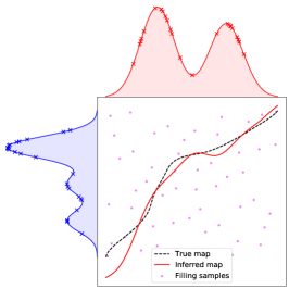
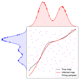
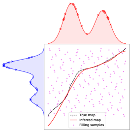
Figure 2: Effect of increasing the number of filling samples $\ell$ on the transportation map. (left): $\ell=50,{n_{\mu}}={n_{\nu}}=25$, (middle): $\ell=100,n=25$, (right): $\ell=200,{n_{\mu}}={n_{\nu}}=25$.

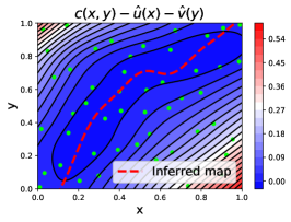
Figure 3: Effect of increasing the number of filling samples $\ell$ on the constraint model. (left): $\ell=50,{n_{\mu}}={n_{\nu}}=25$, (middle): $\ell=100,{n_{\mu}}={n_{\nu}}=25$, (right): true function.

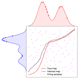
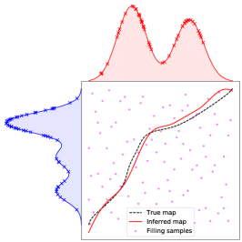
Figure 4: Effect of increasing the number of $\mu$ and $\nu$ samples on the transportation map. (left): $\ell=100,{n_{\mu}}={n_{\nu}}=10$, (middle): $\ell=100,{n_{\mu}}={n_{\nu}}=25$, (right): $\ell=100,{n_{\mu}}={n_{\nu}}=50$.

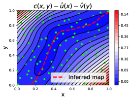
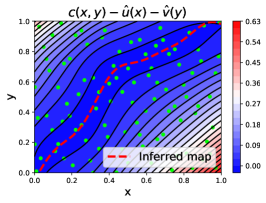
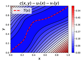
Figure 5: Effect of increasing the number of $\mu$ and $\nu$ samples on the constraint model. (left): $\ell=100,{n_{\mu}}={n_{\nu}}=10$, (middle): $\ell=100,{n_{\mu}}={n_{\nu}}=50$, (right): true function.

1D transportation maps and dual constraint functions.

We illustrate the algorithm described in Theorem F.3 in a 1D setting in Figures 2, 3, 4 and 5, by representing the inferred transportation map $\hat{T}$ obtained from $\hat{u}$, defined as $\hat{T}=x-\nabla_{x}\hat{u}(x)$, and the corresponding constraint function $\hat{h}(x,y)=\frac{1}{2}\|x-y\|^{2}-\hat{u}(x)-\hat{v}(y)$. We sample $x_{1},...,x_{n_{\mu}}$ i.i.d. from $\mu$ and $y_{1},...,y_{n_{\nu}}$ i.i.d. from $\nu$, and use quasi-random samples $(\tilde{x}_{1},\tilde{y}_{1}),...(\tilde{x}_{\ell},\tilde{y}_{\ell})$ from a 2D Sobol sequence (Sobol, 1967), and illustrate the effect of varying $n$, the number of $\mu$ and $\nu$ samples, and $\ell$, the number of space-filling samples. For $k_{X},k_{Y}$ and $k_{XY}$, we use Gaussian kernels $k(x,y)=\exp(-\frac{\|x-y\|^{2}}{2\sigma^{2}})$ of fixed bandwidth $\sigma^{2}=0.1$, and scale the regularization parameters as $\lambda_{1}=\frac{1}{\ell}$ and $\lambda_{2}=\frac{1}{\sqrt{n}}$.

Convergence of $\widehat{\text{OT}}$ to OT.

In Figure 6, we compare $\widehat{\text{OT}}$ to the sampled optimal transport estimator on two 4D truncated Gaussian distributions $\mu$ and $\nu$ s.t. the optimal transportation map from one to another is linear. We progressively increase the number of $\mu$ and $\nu$ samples, averaging on $20$ random draws for each number of samples. The number of filling sample pairs $(\tilde{x}_{i},\tilde{y}_{i})$ is $\ell=100+{n}$, where $n={n_{\mu}}={n_{\nu}}$ is the number samples from $\mu$ and $\nu$. We select the best estimator $\widehat{\text{OT}}$ using a grid search on $(\lambda_{1},\lambda_{2})$. As such, this simulation does not provide a method for selecting those parameters, but rather illustrates that a good pair of parameters exists.

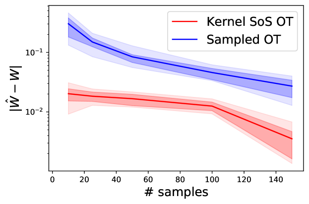
Figure 6: Convergence on 4D truncated Gaussian data with increasing number of samples (left). Full lines correspond to the average mean absolute error (MAE), shaded areas to $25\%-75\%$ and $10\%-90\%$ MAE quantiles. The parameters $\lambda_{1},\lambda_{2}$ are selected via a grid search.

References

- Adams and Fournier (2003) Robert A. Adams and John J. F. Fournier. Sobolev Spaces. Elsevier, 2003.
- Arjovsky et al. (2017) Martin Arjovsky, Soumith Chintala, and Léon Bottou. Wasserstein generative adversarial networks. In International conference on machine learning, pages 214–223. PMLR, 2017.
- Aronszajn (1950) Nachman Aronszajn. Theory of reproducing kernels. Transactions of the American Mathematical Society, 68(3):337–404, 1950.
- Aubin-Frankowski and Szabo (2020) Pierre-Cyril Aubin-Frankowski and Zoltan Szabo. Hard shape-constrained kernel machines. Advances in Neural Information Processing Systems, 33, 2020.
- Bertsekas (2009) Dimitri P. Bertsekas. Convex Optimization Theory. Athena Scientific Belmont, 2009.
- Bonneel et al. (2011) Nicolas Bonneel, Michiel Van De Panne, Sylvain Paris, and Wolfgang Heidrich. Displacement interpolation using Lagrangian mass transport. In Proceedings of the 2011 SIGGRAPH Asia Conference, pages 1–12, 2011.
- Boyd and Vandenberghe (2004) Stephen P. Boyd and Lieven Vandenberghe. Convex Optimization. Cambridge University Press, 2004.
- Brenier (1987) Yann Brenier. Décomposition polaire et réarrangement monotone des champs de vecteurs. CR Acad. Sci. Paris Sér. I Math., 305:805–808, 1987.
- Caffarelli (1992) Luis A. Caffarelli. The regularity of mappings with a convex potential. Journal of the American Mathematical Society, 5(1):99–104, 1992.
- Campbell et al. (2015) Daniel Campbell, Stanislav Hencl, and František Konopeckỳ. The weak inverse mapping theorem. Zeitschrift für Analysis und ihre Anwendungen, 34(3):321–342, 2015.
- Caponnetto and De Vito (2007) Andrea Caponnetto and Ernesto De Vito. Optimal rates for the regularized least-squares algorithm. Foundations of Computational Mathematics, 7(3):331–368, 2007.
- Chen et al. (2018) Liqun Chen, Shuyang Dai, Chenyang Tao, Haichao Zhang, Zhe Gan, Dinghan Shen, Yizhe Zhang, Guoyin Wang, Ruiyi Zhang, and Lawrence Carin. Adversarial text generation via feature-mover’s distance. In Advances in Neural Information Processing Systems 31, pages 4666–4677. 2018.
- Chizat et al. (2020) Lenaic Chizat, Pierre Roussillon, Flavien Léger, François-Xavier Vialard, and Gabriel Peyré. Faster Wasserstein distance estimation with the Sinkhorn divergence. Advances in Neural Information Processing Systems, 33, 2020.
- Cuturi (2013) Marco Cuturi. Sinkhorn distances: Lightspeed computation of optimal transport. In Advances in Neural Information Processing Systems, 2013.
- De Philippis and Figalli (2014) Guido De Philippis and Alessio Figalli. The Monge–Ampère equation and its link to optimal transportation. Bulletin of the American Mathematical Society, 51(4):527–580, 2014.
- Dekel and Leviatan (2004) Shai Dekel and Dany Leviatan. Whitney estimates for convex domains with applications to multivariate piecewise polynomial approximation. Foundations of Computational Mathematics, 4(4):345–368, 2004.
- Feydy et al. (2017) Jean Feydy, Benjamin Charlier, François-Xavier Vialard, and Gabriel Peyré. Optimal Transport for Diffeomorphic Registration. In MICCAI 2017, September 2017.
- Fournier and Guillin (2015) Nicolas Fournier and Arnaud Guillin. On the rate of convergence in Wasserstein distance of the empirical measure. Probability Theory and Related Fields, 162(3-4):707–738, 2015.
- Frogner et al. (2015) Charlie Frogner, Chiyuan Zhang, Hossein Mobahi, Mauricio Araya, and Tomaso A. Poggio. Learning with a Wasserstein loss. In Advances in Neural Information Processing Systems, pages 2053–2061, 2015.
- Genevay et al. (2018) Aude Genevay, Gabriel Peyré, and Marco Cuturi. Learning generative models with Sinkhorn divergences. In International Conference on Artificial Intelligence and Statistics, pages 1608–1617, 2018.
- Genevay et al. (2019) Aude Genevay, Lénaïc Chizat, Francis Bach, Marco Cuturi, and Gabriel Peyré. Sample complexity of Sinkhorn divergences. In The 22nd International Conference on Artificial Intelligence and Statistics, pages 1574–1583, 2019.
- Grave et al. (2019) Edouard Grave, Armand Joulin, and Quentin Berthet. Unsupervised alignment of embeddings with Wasserstein Procrustes. In International Conference on Artificial Intelligence and Statistics (AISTATS), pages 1880–1890. PMLR, 2019.
- Gretton et al. (2012) Arthur Gretton, Karsten M Borgwardt, Malte J Rasch, Bernhard Schölkopf, and Alexander Smola. A kernel two-sample test. The Journal of Machine Learning Research, 13(1):723–773, 2012.
- Grisvard (1985) Pierre Grisvard. Elliptic Problems in Nonsmooth Domains. SIAM, 1985.
- Henrion and Lasserre (2020) Didier Henrion and Jean-Bernard Lasserre. Graph recovery from incomplete moment information, 2020.
- Ho et al. (2017) Nhat Ho, XuanLong Nguyen, Mikhail Yurochkin, Hung Hai Bui, Viet Huynh, and Dinh Phung. Multilevel clustering via Wasserstein means. In International Conference on Machine Learning, pages 1501–1509. PMLR, 2017.
- Hütter and Rigollet (2019) Jan-Christian Hütter and Philippe Rigollet. Minimax rates of estimation for smooth optimal transport maps. arXiv preprint arXiv:1905.05828, 2019.
- Krieg and Sonnleitner (2020) David Krieg and Mathias Sonnleitner. Random points are optimal for the approximation of sobolev functions. arXiv preprint arXiv:2009.11275, 2020.
- Lasserre (2001) Jean Bernard Lasserre. Global optimization with polynomials and the problem of moments. SIAM Journal on Optimization, 11(3):796–817, 2001.
- Lasserre (2009) Jean Bernard Lasserre. Moments, Positive Polynomials and Their Applications. Imperial College Press, 2009.
- Liang (2018) Tengyuan Liang. On how well generative adversarial networks learn densities: Nonparametric and parametric results. arXiv preprint arXiv:1811.03179, 2018.
- Liang (2019) Tengyuan Liang. Estimating certain integral probability metric (IPM) is as hard as estimating under the IPM. arXiv preprint arXiv:1911.00730, 2019.
- Marteau-Ferey et al. (2020) Ulysse Marteau-Ferey, Francis Bach, and Alessandro Rudi. Non-parametric models for non-negative functions. Advances in Neural Information Processing Systems, 2020.
- Mena and Niles-Weed (2019) Gonzalo Mena and Jonathan Niles-Weed. Statistical bounds for entropic optimal transport: sample complexity and the central limit theorem. In Advances in Neural Information Processing Systems, pages 4543–4553, 2019.
- Muandet et al. (2017) Krikamol Muandet, Kenji Fukumizu, Bharath Sriperumbudur, and Bernhard Schölkopf. Kernel Mean Embedding of Distributions: A Review and Beyond, volume 10. Now Foundations and Trends, 2017.
- Narcowich et al. (2005) Francis Narcowich, Joseph Ward, and Holger Wendland. Sobolev bounds on functions with scattered zeros, with applications to radial basis function surface fitting. Mathematics of Computation, 74(250):743–763, 2005.
- Nemirovski (2004) Arkadi Nemirovski. Interior point polynomial time methods in convex programming. Lecture notes, 2004.
- Nesterov and Nemirovskii (1994) Yurii Nesterov and Arkadii Nemirovskii. Interior-Point Polynomial Algorithms in Convex Programming. Society for Industrial and Applied Mathematics, 1994.
- Niles-Weed and Rigollet (2019) Jonathan Niles-Weed and Philippe Rigollet. Estimation of Wasserstein distances in the spiked transport model. arXiv preprint 1909.07513, 2019.
- Parrilo (2003) Pablo A Parrilo. Semidefinite programming relaxations for semialgebraic problems. Mathematical programming, 96(2):293–320, 2003.
- Peyré and Cuturi (2019) Gabriel Peyré and Marco Cuturi. Computational optimal transport. Foundations and Trends® in Machine Learning, 11(5-6):355–607, 2019.
- Redko et al. (2019) Ievgen Redko, Nicolas Courty, Rémi Flamary, and Devis Tuia. Optimal transport for multi-source domain adaptation under target shift. In The 22nd International Conference on Artificial Intelligence and Statistics, pages 849–858. PMLR, 2019.
- Reznikov and Saff (2016) A. Reznikov and E. B. Saff. The covering radius of randomly distributed points on a manifold. International Mathematics Research Notices, 2016(19):6065–6094, 2016.
- Rockafellar (1970) R. Tyrrell Rockafellar. Convex Analysis, volume 36. Princeton University Press, 1970.
- Rosasco et al. (2010) Lorenzo Rosasco, Mikhail Belkin, and Ernesto De Vito. On learning with integral operators. Journal of Machine Learning Research, 11(2), 2010.
- Rudi et al. (2020) Alessandro Rudi, Ulysse Marteau-Ferey, and Francis Bach. Finding global minima via kernel approximations. In Arxiv preprint arXiv:2012.11978, 2020.
- Salimans et al. (2018) Tim Salimans, Dimitris Metaxas, Han Zhang, and Alec Radford. Improving GANs using optimal transport. In 6th International Conference on Learning Representations, ICLR 2018, 2018.
- Santambrogio (2015) Filippo Santambrogio. Optimal Transport for Applied Mathematicians: Calculus of Variations, PDEs, and Modeling. Progress in Nonlinear Differential Equations and Their Applications. Springer International Publishing, 2015.
- Sobol (1967) Ilya Meerovich Sobol. On the distribution of points in a cube and the approximate evaluation of integrals. Zhurnal Vychislitel’noi Matematiki i Matematicheskoi Fiziki, 7(4):784–802, 1967.
- Steinwart and Christmann (2008) Ingo Steinwart and Andreas Christmann. Support Vector Machines. Springer Science & Business Media, 2008.
- Tolstikhin et al. (2018) I Tolstikhin, O Bousquet, S Gelly, and B Schölkopf. Wasserstein auto-encoders. In 6th International Conference on Learning Representations (ICLR 2018). OpenReview. net, 2018.
- Weed and Bach (2019) Jonathan Weed and Francis Bach. Sharp asymptotic and finite-sample rates of convergence of empirical measures in Wasserstein distance. Bernoulli, 25(4A):2620–2648, 2019.
- Weed and Berthet (2019) Jonathan Weed and Quentin Berthet. Estimation of smooth densities in Wasserstein distance. In Conference on Learning Theory, pages 3118–3119, 2019.
- Wendland (2004) Holger Wendland. Scattered Data Approximation, volume 17. Cambridge University Press, 2004.
- Wendland and Rieger (2005) Holger Wendland and Christian Rieger. Approximate interpolation with applications to selecting smoothing parameters. Numer. Math., 101(4):729–748, October 2005.
- Xu et al. (2018) Hongteng Xu, Wenlin Wang, Wei Liu, and Lawrence Carin. Distilled Wasserstein learning for word embedding and topic modeling. In Advances in Neural Information Processing Systems 31, pages 1716–1725. 2018.