Canonical transformations generated by the boundary volume:
Unimodular and non-Abelian teleparallel gravity

Abstract

Recently, a new choice of variables was identified to understand how the quantum group structure appeared in three-dimensional gravity Dupuis:2020ndx . These variables are introduced via a canonical transformation generated by a boundary term. We show that this boundary term can actually be taken to be the volume of the boundary and that the new variables can be defined in any dimension greater than three. In addition, we study the associated metric and teleparallel formalisms. The former is a variant of the Henneaux–Teitelboim model for unimodular gravity. The latter provides a non-Abelian generalization of the usual Abelian teleparallel formulation.

I Introduction

Quantum states are built from the representations of the symmetries, identified at the classical level. The structure of the symmetries depends on the choice of variables used to describe the phase space of the classical theory. In the gravity case, moving from the metric to the frame field variables (Palatini formalism) enlarges the set of gauge symmetries since internal Lorentz rotations are absent in the usual metric formalism. On the other hand, treating gravity as a constrained topological field theory Freidel:1999rr ; Freidel:2015gpa has the opposite effect: the topological theory has a larger symmetry algebra. Gravity is recovered by imposing constraints that break the gauge symmetries down to those that appear in general relativity. Using the teleparallel formulation of gravity leads to yet another different type of symmetries, representing different representations at the quantum level (possibly related by dualities). Since both the metric and teleparallel formulations can be seen as a second-order formulation of gravity, it is interesting to study the relationship between the respective symmetries depending on the choice of variables. We refer to Freidel:2020xyx ; Freidel:2020svx ; Freidel:2020ayo ; DePaoli:2018erh ; Oliveri:2019gvm ; Wieland:2020gno ; Wieland:2017zkf ; Wieland:2017cmf ; Wieland:2018ymr for a recent discussion about these different issues in gravity.

In field theory, canonical transformations are typically generated by adding topological invariants or boundary terms to the action. Let us list some important examples in the context of gravity below (a more detailed discussion can be found in e.g. Freidel:2020xyx ; Freidel:2020svx ; Freidel:2020ayo ; DePaoli:2018erh ; Oliveri:2019gvm ; Wieland:2020gno ; Wieland:2017zkf ; Wieland:2017cmf ; Wieland:2018ymr and references therein).

• In any dimension, the Gibbons-Hawking-York (boundary) term generates the canonical transformation changing the polarization from the superspace momentum representation, where the wave-functionals depend on the ADM momentum $\tilde{\pi}^{ab}=\frac{1}{16\pi G}\sqrt{\det{h}}\,(K^{ab}-h^{ab}K)$, to the position representation, where the wave-functional $\Psi[h_{ab}]$ depends only on the intrinsic metric of the boundary, c.f. adm ; kiefer ; thiemann .

• For gravity in four spacetime dimensions, the Holst term induces the Ashtekar–Barbero canonical transformation from the ADM-type of variables to the (complex) Ashtekar variables, which greatly simplifies the structure of the constraints, enabling the loop quantization of gravity newvariables ; Barbero1994 ; holst-action ; thiemann .

• In three-dimensions, quantum groups play an important role in both the quantization of Chern–Simons theory Fock:1998nu and the discrete path integral formulation TV of gravity. Quantum groups appear as deformed gauge symmetries, where the quantum deformation is parametrized by the cosmological constant. This is in striking contrast to the classical formulation of three-dimensional gravity in the first-order formalism, where the gauge symmetries do not depend on the cosmological constant. It was recently found that a canonical transformation, induced by a boundary term, could be used to have a (bulk) theory defined in terms of new variables, such that the gauge symmetries do depend now on the cosmological constant as well, see Dupuis:2020ndx . This provided a direct manner to retrieve the quantum group symmetries upon quantization.

It has been conjectured that quantum groups could also be relevant for quantum gravity in four dimensions Smolin:2002sz ; Fairbairn:2010cp ; Han:2010pz , so one might wonder whether the canonical transformation or the boundary term that was identified in Dupuis:2020ndx can also be introduced in four dimensions. We show here that this is indeed the case and that there is a straightforward generalization of the boundary term in the first-order formalism. It is then natural to ask what happens to the second-order formalism and how the metric and teleparallel formulations of gravity could be expressed in terms of the new variables. Here, we answer these questions. In the metric formalism, we have a new notion of the Christoffel symbol. The volume term that is added to the action via the cosmological constant is replaced by the divergence of a vector field, whose norm depends on the cosmological constant. In fact, we recover a variant of the Henneaux–Teitelboim model for unimodular gravity Henneaux:1989zc . On the other hand, in the teleparallel formalism tele , the new variables suggest a deformed notion of torsion, which defines a new and non-Abelian version of the standard teleparallel formulation.

The boundary term that generates the canonical transformation that was introduced in Dupuis:2020ndx depends on an internal vector $r^{I}$, whose norm sets the value of the cosmological constant. In order to not increase the number of degrees of freedom, it was assumed that the vector is an auxiliary background structure, whose field-variations vanish on the covariant phase space, i.e. $\delta[r^{I}]=0$. However, the boundary term Dupuis:2020ndx has a very strong resemblance with the volume term of the boundary. It seems natural, therefore, to relax the condition $\delta[r^{I}]=0$. In fact, we will show that if we actually interpret the vector $r^{I}$ as the internal normal $n^{I}$ to the boundary, the generating functional Dupuis:2020ndx is exactly the volume of the boundary. In here, we show that given this interpretation, we can allow for $\delta[n^{I}]\neq 0$ and still perform the canonical transformation, without adding any new degrees of freedom in the bulk.

The new formulation has some interesting relations with already existing frameworks.

• The boundary term plays an important role in holographic renormalization Bianchi:2001kw ; Skenderis:2002wp so that our new variables will also be relevant to this framework.

• With the change of variables, the volume term that scales with the cosmological constant drops out of the action and is replaced by the divergence of a vector field and a constraint which sets the cosmological constant as the norm of this vector field. We will see below that the resulting action defines a variation of the Henneaux–Teitelboim model for unimodular gravity Henneaux:1989zc .

One can often see the first-order formalism for gravity as a gauge theory, so that the canonical variables are Lie algebra-valued differential forms. This is obviously realized in three dimension in the Chern–Simons formulation. In four dimensions, the McDowell–Mansouri formulation MacDowell:1977jt provides a similar realization. Depending on the value of the cosmological constant and the signature of the metric, one usually deals with a (anti-)de Sitter or Poincaré (or Euclidian) gauge group, where the frame field has values in the boost or translation sector of the group. Accordingly, the (anti-)de Sitter or Poincaré curvature splits into the Lorentzian curvature sector, which depends on the cosmological constant, and the translational or boost sector, which represents torsion and is independent of $\Lambda$. Since the (anti-)de Sitter or Poincaré groups can be seen as the semi-cross product between the Lorentz transformations and the boosts or translations, there is a natural action of the Lorentz group on the frame field. On the other hand, there is no action of translations back onto rotations (the commutator of a translation and a rotation has no translational part).

The canonical transformation that we will study in here amounts to choosing a different decomposition of the (anti-)de Sitter group (the Poincaré case can also be treated in the same way). Indeed, if the standard formulation amounts to use the Cartan decomposition, then the canonical transformation instead picks the Iwasawa decomposition. We have then a double cross product relation and a more symmetric treatment between the connection and the frame field: the connection acts on the frame field, and the frame field acts back on the connection. As a consequence the (anti-)de Sitter or Poincaré curvature can be split differently than before. We get a generalized notion of torsion, which can be viewed as a (non-Abelian) curvature in the frame field sector. This is especially relevant regarding the teleparallel formulation.

We finally note that the boundary term could also be added in the usual metric formulation of General Relativity. We expect that this new boundary term will induce a canonical transformation from pure metric gravity to a version of unimodular gravity, similar to the one introduced in this paper. Since we are primarily interested in approaches to quantum gravity based on the first-order formalism, we do not explore this thread in this paper.

Outline:

The article is organized as follows. In section II, we review the gauge theory framework when dealing with a matched pair (double cross product) of Lie algebras, which will conveniently set up the conventions for the rest of the paper. In section III, we discuss how the canonical transformation can be implemented in any dimension by the boundary term given in terms of the volume of the boundary. In section IV.1, we determine the metric formulation in the new variables, while in section IV.2, we determine the dual teleparallel formulation.

II Gauge theory for a matched pair of Lie groups

In the following, we develop the notion of a gauge theory for a matched pair of Lie algebras. This structure generalizes the more common semi-direct product that can be found in the Poincaré case or in the decomposition of the Lorentz group in terms of rotations and boosts (although they do not form a Lie algebra). Matched pairs are the relevant structure which gives rise to the quantum group structure at the quantum level. For example, in the three-dimensional gravity case. A reader who would be more geometry inclined can skip this section, which nevertheless emphasizes that what is called torsion can also be viewed as a type of curvature.

The algebraic background behind the matched pairs can be found in Majid:1996kd . We call a matched pair ${\mathfrak{G}}={\mathfrak{g}}\bowtie{\mathfrak{h}}$ of Lie algebras the pair of Lie algebras ${\mathfrak{g}}$ and ${\mathfrak{h}}$, with respective Lie brackets $[\cdot,\cdot]_{\mathfrak{g}}$ and $[\cdot,\cdot]_{\mathfrak{h}}$, equipped with two bilinear maps $\lhd:{\mathfrak{h}}\times{\mathfrak{g}}\rightarrow{\mathfrak{h}},(x,\alpha)\mapsto x\lhd\alpha$ and $\rhd:{\mathfrak{h}}\times{\mathfrak{g}}\rightarrow{\mathfrak{g}},(x,\alpha)\mapsto x\rhd\alpha$, such that ${\mathfrak{h}}$ is a right ${\mathfrak{g}}$-module and ${\mathfrak{g}}$ is a left ${\mathfrak{h}}$-module. More intuitively, ${\mathfrak{g}}$ acts from the right on ${\mathfrak{h}}$ via $\lhd$ and there is a back action $\rhd$ of ${\mathfrak{h}}$ on ${\mathfrak{g}}$. To guarantee the Jacobian identity on ${\mathfrak{G}}$, the left and right actions must satisfy the following compatibility conditions: $\forall\alpha,\beta\in{\mathfrak{g}},\,x,y\in{\mathfrak{h}}$,

$$x\rhd[\alpha,\beta]_{\mathfrak{g}} =[x\rhd\alpha,\beta]_{\mathfrak{g}}+[\alpha,x\rhd\beta]_{\mathfrak{g}}+(x\lhd\alpha)\rhd\beta-(x\lhd\beta)\rhd\alpha,$$ (1a)

$$[x,y]_{\mathfrak{h}}\lhd\alpha =[x\lhd\alpha,y]_{\mathfrak{h}}+\,[x,y\lhd\alpha]_{\mathfrak{h}}+\,x\lhd(y\rhd\alpha)-y\lhd(x\rhd\alpha).$$ (1b)

As a vector space, ${\mathfrak{g}}\bowtie{\mathfrak{h}}$ is isomorphic to ${\mathfrak{g}}\oplus{\mathfrak{h}}$. If we introduce a matched basis, such that $(\alpha,x)\in{\mathfrak{g}}\oplus{\mathfrak{h}}\sim{\mathfrak{g}}\bowtie{\mathfrak{h}}$, we may express the Lie bracket of ${\mathfrak{G}}$ in terms of $[\cdot,\cdot]_{\mathfrak{g}}$, $[\cdot,\cdot]_{\mathfrak{h}}$, $\lhd$ and $\rhd$,

$$\big{[}(\alpha,x),(\beta,y)\big{]}\equiv\big{(}[\alpha,\beta]_{\mathfrak{g}}+x\rhd\beta-y\rhd\alpha,\,[x,y]_{\mathfrak{h}}+x\lhd\beta-y\lhd\alpha\big{)},\quad\forall\alpha,\beta\in{\mathfrak{g}},\quad x,y\in{\mathfrak{h}}.$$ (2)

In particular, there is the mixed bracket

$$\big{[}(0,x),(\beta,0)\big{]}\equiv[x,\beta]=x\lhd\beta+x\rhd\beta\in{\mathfrak{g}}\oplus{\mathfrak{h}}.$$ (3)

Notice that the left and right modules can be written in terms of the Lie bracket alone,

$$x\lhd\beta:=[x,\beta]\big{|}_{{{\mathfrak{h}}}},\quad x\rhd\beta:=[x,\beta]\big{|}_{{{\mathfrak{g}}}},$$ (4)

where $[x,\beta]|_{{V}}$ is the projection of the Lie bracket $[\cdot,\cdot]$ on the vector space $V$. With this notation, the compatibility relations (1) become

$$x\rhd[\alpha,\beta]_{\mathfrak{g}} =\big{[}[x,\alpha]\big{|}_{{{\mathfrak{g}}}},\beta\big{]}_{\mathfrak{g}}+\big{[}\alpha,[x,\beta]\big{|}_{{{\mathfrak{g}}}}\big{]}_{\mathfrak{g}}+\big{[}[x,\alpha]\big{|}_{{{\mathfrak{h}}}},\beta\big{]}\big{|}_{{{\mathfrak{g}}}}-\big{[}[x,\beta]\big{|}_{{{\mathfrak{h}}}},\alpha\big{]}\big{|}_{{{\mathfrak{g}}}},$$ (5a)

$$[x,y]_{\mathfrak{h}}\lhd\alpha =\big{[}[x,\alpha]\big{|}_{{{\mathfrak{h}}}},y\big{]}_{\mathfrak{h}}+\big{[}x,[y,\alpha]\big{|}_{{{\mathfrak{h}}}}\big{]}_{\mathfrak{h}}+\big{[}x,[y,\alpha]\big{|}_{{{\mathfrak{g}}}}\big{]}\big{|}_{{{\mathfrak{h}}}}-\big{[}y,[x,\alpha]\big{|}_{{{\mathfrak{g}}}}\big{]}\big{|}_{{{\mathfrak{h}}}}.$$ (5b)

Consider then a gauge connection $\boldsymbol{A}$ for such a Lie algebra, i.e. a ${\mathfrak{G}}$-valued one-form on a manifold $\mathcal{M}$, and consider its different components with respect to the matched Lie algebra ${\mathfrak{g}}\bowtie{\mathfrak{h}}$. This type of gauge theory was studied by Majid Majid:1996kd at the discrete level of parallel propagators (holonomies). Below we will derive the infinitesimal picture.

Let us denote by $\gamma$ and $h$ the components of such a gauge connection with respect to the Lie algebras ${\mathfrak{g}}$ and ${\mathfrak{h}}$. The ${\mathfrak{g}}\bowtie{\mathfrak{h}}$ Lie algebra-valued gauge connection takes the form

$$\boldsymbol{A}=\gamma+h\in({\mathfrak{g}}\oplus{\mathfrak{h}})\otimes\Lambda^{1}(M).$$ (6)

Due to the kick-back action between ${\mathfrak{g}}$ and ${\mathfrak{h}}$, there is a non-trivial mixing between the components of the ${\mathfrak{g}}\bowtie{\mathfrak{h}}$ basis, see (4). Consider, for example, a ${\mathfrak{G}}$-valued $p$-form $\boldsymbol{B}=(\beta,b)$. Its exterior covariant derivative is

$$\mathrm{d}_{\boldsymbol{A}}\boldsymbol{B} = \mathrm{d}\beta+\mathrm{d}b+[\gamma+h,\beta+b]=\mathrm{d}\beta+\mathrm{d}b+[\gamma,\beta]_{{\mathfrak{g}}}+[\gamma,b]+[h,b]_{{\mathfrak{h}}}+[h,\beta]$$ (7)

$$= \left(\mathrm{d}\beta+[\gamma,\beta]_{{\mathfrak{g}}}+[\gamma,b]\big{|}_{{{\mathfrak{g}}}}+[h,\beta]\big{|}_{{{\mathfrak{g}}}}\right)+\left(\mathrm{d}b+[h,b]_{{\mathfrak{h}}}+[\gamma,b]\big{|}_{{{\mathfrak{h}}}}+[h,\beta]\big{|}_{{{\mathfrak{h}}}}\right).$$

For the individual component fields $(\beta,0)$ and $(0,b)$, we have the covariant derivatives

$$\boldsymbol{D}_{|{{\mathfrak{g}}}}\beta =\mathrm{d}\beta+[\gamma,\beta]_{{\mathfrak{g}}}+[h,\beta]\big{|}_{{{\mathfrak{g}}}},$$ (8)

$$\boldsymbol{D}_{|{{\mathfrak{h}}}}b =\mathrm{d}b+[\gamma,b]\big{|}_{{{\mathfrak{h}}}}+[h,b]_{{\mathfrak{h}}}.$$ (9)

Due to the kick-back actions between the two Lie algebras, the covariant derivatives depend on both connection components $\gamma$ and $h$. Consider then the components of the field strength $\boldsymbol{F}$ in the directions of ${\mathfrak{g}}$ and ${\mathfrak{h}}$,

$$\boldsymbol{F}[\boldsymbol{A}] = \mathrm{d}\boldsymbol{A}+{\frac{1}{2}}[\boldsymbol{A}\wedge\boldsymbol{A}]=\mathrm{d}\gamma+\mathrm{d}h+{\frac{1}{2}}\big{[}(\gamma+h)\wedge(\gamma+h)\big{]}$$ (10)

$$= \mathrm{d}\gamma+\mathrm{d}h+{\frac{1}{2}}[\gamma\wedge\gamma]_{{{\mathfrak{g}}}}+[\gamma\wedge h]\big{|}_{{{{\mathfrak{g}}}}}+[\gamma\wedge h]\big{|}_{{{{\mathfrak{h}}}}}+{\frac{1}{2}}[h\wedge h]_{{{{\mathfrak{h}}}}}$$

$$= \left(\mathrm{d}\gamma+{\frac{1}{2}}[\gamma\wedge\gamma]_{{{\mathfrak{g}}}}+[\gamma\wedge h]\big{|}_{{{{\mathfrak{g}}}}}\right)+\left(\mathrm{d}h+[\gamma\wedge h]\big{|}_{{{{\mathfrak{h}}}}}+{\frac{1}{2}}[h\wedge h]_{{{{\mathfrak{h}}}}}\right)\equiv{\cal F}+{\cal T}.$$

The physical significance of splitting $\boldsymbol{F}$ into ${\cal F}\in{\mathfrak{g}}\otimes\Lambda^{2}(\mathcal{M})$ and ${\cal T}\in{\mathfrak{h}}\otimes\Lambda^{2}(\mathcal{M})$ will be clear below. We will identify, in fact, ${\cal F}$ and ${\cal T}$ with a deformed version of ${\mathfrak{h}}$-valued torsion and ${\mathfrak{g}}$-valued curvature,

$${\cal F} =\mathrm{d}\gamma+{\frac{1}{2}}[\gamma\wedge\gamma]_{{\mathfrak{g}}}+[\gamma\wedge h]\big{|}_{{\mathfrak{g}}}\equiv F+[\gamma\wedge h]\big{|}_{{\mathfrak{g}}},$$ (11)

$${\cal T} =\mathrm{d}h+[\gamma\wedge h]\big{|}_{{\mathfrak{h}}}+{\frac{1}{2}}[h\wedge h]_{{\mathfrak{h}}}\equiv T+{\frac{1}{2}}[h\wedge h]_{{\mathfrak{h}}}.$$ (12)

Again, the curvature components depend on both connection types. The Bianchi identity for each component is

$$0=\mathrm{d}_{\boldsymbol{A}}\boldsymbol{F} = \mathrm{d}{\cal F}+\mathrm{d}{\cal T}+\big{[}(\gamma+h)\wedge({\cal F}+{\cal T})\big{]}$$ (13)

$$= \left(\mathrm{d}{\cal F}+[\gamma\wedge{\cal F}]_{{\mathfrak{g}}}\,+[h\wedge{\cal F}]\big{|}_{{{\mathfrak{g}}}}+[\gamma\wedge{\cal T}]\big{|}_{{{\mathfrak{g}}}}\right)+\left(\mathrm{d}{\cal T}+[\gamma\wedge{\cal T}]_{{\mathfrak{h}}}\,+[h\wedge{\cal F}]\big{|}_{{{\mathfrak{h}}}}+[\gamma\wedge{\cal T}]\big{|}_{{{\mathfrak{h}}}}\right).$$

Let us consider then the gauge transformations of such a ${\mathfrak{G}}$-valued connection. Let $\boldsymbol{\lambda}=(\phi,t)$ be a ${\mathfrak{G}}$-valued scalar, which generates an infinitesimal transformation of the connection $\boldsymbol{A}=(\gamma,h)$,

$$\delta_{\boldsymbol{\lambda}}[\boldsymbol{A}] = \mathrm{d}\boldsymbol{\lambda}+[\boldsymbol{A},\boldsymbol{\lambda}]=\left(\mathrm{d}\phi+[\gamma,\phi]_{{\mathfrak{g}}}+[h,\phi]\big{|}_{{{\mathfrak{g}}}}+[\gamma,t]\big{|}_{{{\mathfrak{g}}}}\right)+\left(\mathrm{d}t+[h,t]_{{\mathfrak{h}}}+[\gamma,t]\big{|}_{{{\mathfrak{h}}}}+[h,\phi]\big{|}_{{{\mathfrak{h}}}}\right).$$ (14)

For pure rotations ($t=0$) and pure translations ($\phi=0$), we find

$$\left.\begin{array}[]{rlrl}\delta_{\phi}[\gamma]&=\mathrm{d}\phi+[\gamma,\phi]_{{\mathfrak{g}}}+[h,\phi]\big{|}_{{{\mathfrak{g}}}}=\boldsymbol{D}_{|{\mathfrak{g}}}\phi,&\delta_{\phi}[h]&=[h,\phi]\big{|}_{{{\mathfrak{h}}}},\\ \delta_{t}[\gamma]&=[\gamma,t]\big{|}_{{{\mathfrak{g}}}},&\delta_{t}[h]&=\mathrm{d}t+[h,t]_{{\mathfrak{h}}}+[\gamma,t]\big{|}_{{{\mathfrak{h}}}}=\boldsymbol{D}_{|{\mathfrak{h}}}t.\end{array}\hskip 5.0pt\right\}$$ (15)

What is nice about these transformations is that the variation of $\gamma$ or $h$ in each of the different components is either a commutator or a derivative. In other words, the two components of the curvature two-form behave completely analogous under gauge transformations. Since $\delta_{\boldsymbol{\lambda}}[\boldsymbol{F}]=[\boldsymbol{F},\boldsymbol{\lambda}]$, we obtain

$$[{\cal F}+{\cal T},\phi+t] = [{\cal F},\phi]_{\mathfrak{g}}+[{\cal F},t]\big{|}_{{{\mathfrak{g}}}}+[{\cal T},\phi]\big{|}_{{\mathfrak{g}}}+[{\cal T},t]_{\mathfrak{h}}+[{\cal F},t]\big{|}_{{\mathfrak{h}}}+[{\cal T},\phi]\big{|}_{{\mathfrak{h}}}\,.$$ (16)

In other words,

$$\left.\begin{array}[]{rlrl}\delta_{\phi}[{\cal F}]&=[{\cal F},\phi]_{\mathfrak{g}}+[{\cal T},\phi]\big{|}_{{\mathfrak{g}}},&\delta_{\phi}[{\cal T}]&=[{\cal T},\phi]\big{|}_{{\mathfrak{h}}}\\ \delta_{t}[{\cal F}]&=[{\cal F},t]\big{|}_{{{\mathfrak{g}}}},&\delta_{t}[{\cal T}]&=[{\cal T},t]_{\mathfrak{h}}+[{\cal F},t]\big{|}_{{\mathfrak{h}}}.\end{array}\hskip 5.0pt\right\}$$ (17)

A simple, but non trivial, example of such a matched pair of Lie algebras is the Poincaré Lie algebra. It is a semi-cross product ${\mathfrak{G}}={\mathfrak{g}}{\rhd\!\!\!<}{\mathfrak{h}}$, where ${\mathfrak{g}}$ is either of the Lie algebra $\mathfrak{so}(n)$ or $\mathfrak{so}(n-1,1)$, depending on the signature of spacetime, and ${\mathfrak{h}}\sim\mathbb{R}^{n}$ is the Abelian Lie algebra of translations on $\mathbb{R}^{n}$. The respective generators are the generators of (Lorentz) rotations $J_{MN}=-J_{NM}$ and translations $P_{M}$, which are labelled by spacetime indices $M,N,\dots=1,\dots,n$.

In the Poincaré context, there is no kick-back action of ${\mathfrak{h}}$ on ${\mathfrak{g}}$ (recall $[J,P]\propto P$). Given (4), we thus have

$$(\phi,t)\in{\mathfrak{g}}{\rhd\!\!\!<}{\mathfrak{h}},\quad t\lhd\phi:=[t,\phi]\big{|}_{{{\mathfrak{h}}}},\quad t\rhd\phi:=[t,\phi]\big{|}_{{{\mathfrak{g}}}}=0.$$ (18)

The translations commute, i.e. $[\cdot,\cdot]_{{\mathfrak{h}}}=0$, and the covariant derivative for the component fields $(\phi,0)$ and $(0,t)$ with values in ${\mathfrak{g}}$ or ${\mathfrak{h}}$ is given by

$$\boldsymbol{D}_{|{\mathfrak{g}}}\phi=\mathrm{d}\phi+[\gamma,\phi]_{{\mathfrak{g}}},\quad\boldsymbol{D}_{|{\mathfrak{h}}}t=\mathrm{d}t+[\gamma,t]\big{|}_{{{\mathfrak{h}}}}.$$ (19)

Consider then the components of the curvature two-form $\boldsymbol{F}$ in the rotational and translational directions ${\mathfrak{g}}$ and ${\mathfrak{h}}$ of the Poincaré Lie algebra,

$$\boldsymbol{F}[\boldsymbol{A}] = \left(\mathrm{d}\gamma+{\frac{1}{2}}[\gamma\wedge\gamma]_{{{\mathfrak{g}}}}\right)+\left(\mathrm{d}h+[\gamma\wedge h]\big{|}_{{{{\mathfrak{h}}}}}\right)=F+T.$$ (20)

We recognize the usual notion of curvature $F$ and torsion $T$, provided we identify $\gamma$ with the spin connection $\omega$ and $h$ with the frame field $e$.

The infinitesimal gauge transformations for pure rotations ($t=0$) and pure translations ($\phi=0$) are

$$\begin{array}[]{rlrl}\delta_{\phi}[\gamma]&=\mathrm{d}\phi+[\gamma,\phi]_{{\mathfrak{g}}}=\boldsymbol{D}_{|{\mathfrak{g}}}\phi,&\quad\delta_{\phi}[h]&=[h,\phi]\big{|}_{{{\mathfrak{h}}}},\\ \delta_{t}[\gamma]&=0,&\delta_{t}[h]&=\mathrm{d}t+[\gamma,t]\big{|}_{{{\mathfrak{h}}}}=\boldsymbol{D}_{|{\mathfrak{h}}}t,\end{array}$$ (21)

where $\delta_{\phi}[\gamma]$ is the $\mathfrak{so}$ gauge transformation for the spin connection $\omega=\gamma$, and $\delta_{t}[h]$ is an infinitesimal translation of the frame field $h=e$. Finally, there are the Poincaré transformations of the curvature two-form

$$\begin{array}[]{rlrl}\delta_{\phi}[F]&=[F,\phi]_{\mathfrak{g}},&\qquad\delta_{\phi}[T]&=[T,\phi]\big{|}_{{\mathfrak{h}}}\\ \delta_{t}[F]&=0,&\qquad\delta_{t}[T]&=[F,t]\big{|}_{{\mathfrak{h}}}.\end{array}$$ (22)

Although the translations $t\in{\mathfrak{h}}$ are Abelian, a general such translation will act non-trivially on the translational curvature (torsion). If we would choose, however, a connection $\gamma$ such that $F[\gamma]=0$, both the torsion component $T$ and the rotational (Lorentz) component $F$ of the Poincaré connection would be translational invariant. This choice underlies the teleparallel equivalent of general relativity.

In the following, we will consider the more complicated case of ${\mathfrak{G}}=\mathfrak{so}(n-1,1)\sim\mathfrak{so}(n-1)\bowtie\mathfrak{an}_{n-1}$, which is an example of a matched Lie algebra induced by the Iwasawa decomposition of the Lorentz Lie algebra $\mathfrak{so}(n,1)$.

III Canonical transformation induced by the boundary volume term

III.1 Warm up: three-dimensions

Consider the three-dimensional Einstein – Cartan action in first-order spin-connection variables with a cosmological constant $\Lambda$, together with the following boundary terms, whose significance will become clear below,

$$S_{{\text{EC}}}[e,A|n] =\frac{1}{16\pi G}\bigg{[}\int_{\mathcal{M}}{\varepsilon_{IJK}\,e^{K}\wedge\Big{(}R^{IJ}[A]-\frac{\Lambda}{3}e^{I}\wedge e^{J}\Big{)}}$$

$$\hskip 70.0001pt-2\int_{\partial\mathcal{M}}\Big{(}s\,\varepsilon_{IJK}e^{K}\wedge n^{I}\mathrm{d}_{A}n^{J}+\frac{\sqrt{|\Lambda|}}{2}\varepsilon_{IJK}n^{K}e^{I}\wedge e^{J}\Big{)}\bigg{]}.$$ (23)

The action in the bulk is a functional of the Lorentz curvature $\tensor{R}{{}^{I}_{J}}[A]=\mathrm{d}\tensor{A}{{}^{I}_{J}}+\tensor{A}{{}^{I}_{K}}\wedge\tensor{A}{{}^{K}_{J}}$ and the triad $e^{I}$. The boundary term consists of two parts. The first term is the usual Gibbons – Hawking – York boundary term for first-order spin connection variables, where $\mathrm{d}_{A}[\cdot]=\mathrm{d}[\cdot]+[A,\cdot]$ is the covariant exterior derivative. The internal vector field $n^{I}$ is constrained to lie orthogonal to the boundary, i.e. $n_{I}\varphi_{\partial\mathcal{M}}^{\ast}e^{I}=0$, where $\varphi_{\partial\mathcal{M}}^{\ast}:T^{\ast}\mathcal{M}\rightarrow T^{\ast}{\partial\mathcal{M}}$ is the pull-back. In addition, $n^{I}$ is normalized such that $s=\eta_{IJ}n^{I}n^{J}=n_{I}n^{I}=\{\pm 1,0\}$, depending on whether the boundary is spacelike, timelike, or null. Its orientation is such that $n^{a}:=n^{I}\tensor{e}{{}_{I}^{a}}$ is the outwardly oriented normal to the boundary. If the torsionless equation is satisfied, then the first term is the integral of the trace of the extrinsic curvature. The second term is proportional to the induced volume of the boundary. The boundary conditions are

$$\tensor{h}{{}^{I}_{J}}\varphi^{\ast}_{\partial\mathcal{M}}\delta[e^{J}]=0,\qquad\varphi^{\ast}_{\partial\mathcal{M}}\delta[n_{I}e^{I}]=0,$$ (24)

where $\delta[\cdot]$ is a variation on the infinite-dimensional space of kinematical histories, and $h_{IJ}=-sn_{I}n_{J}+\eta_{IJ}$ is the internal projector onto the boundary.

It is also useful to evaluate the action (23) for a spin connection $\tensor{A}{{}^{I}_{J}}$, which is torsionless (by going half-shell). We obtain

$$S_{\text{EC}}[A,e|n]\Big{|}_{\mathrm{d}_{A}e=0}=S_{\text{EH}}[g|n]=\frac{1}{16\pi G}\left[\int_{\mathcal{M}}d^{3}v\big{(}R[g]-2\Lambda\big{)}+2\int_{\partial\mathcal{M}}d^{2}v\big{(}sK-\sqrt{|\Lambda|}\big{)}\right],$$ (25)

where $R[g]$ is the Ricci scalar for the metric $g_{ab}=e_{Ia}\tensor{e}{{}^{I}_{b}}$, and $K=\nabla_{a}n^{a}$ is the trace of the extrinsic curvature. In addition, $d^{3}v$ and $d^{2}v$ are the canonical volume elements on $\mathcal{M}$ and $\partial{\mathcal{M}}$. The volume term appears in the definition of the bulk plus boundary action (25) to cancel infrared divergencies that would otherwise appear when the boundary $\partial\mathcal{M}$ is sent to infinity Bianchi:2001kw .

Consider then a region $\Sigma\subset\partial\mathcal{M}$ within the boundary. The first variation of the action for given boundary conditions (24) determines the pre-symplectic potential $\Theta_{\Sigma}^{\text{EC}}$ on the space of physical histories, i.e. the space of solutions to the field equations. A straightforward calculation gives

$$\Theta^{\text{EC}}_{\Sigma}(\delta)=\frac{1}{8\pi G}\int_{\Sigma}\Big{(}s\,\varepsilon_{IJ}\delta[e^{I}]\wedge K^{J}-\sqrt{|\Lambda|}\,\varepsilon_{IJ}e^{I}\wedge\delta[e^{J}]\Big{)}-\frac{1}{8\pi G}\oint_{\partial\Sigma}s\,\varepsilon_{IJ}e^{I}\delta[n^{J}],$$ (26)

where $K^{I}=\varphi^{\ast}_{\partial M}\mathrm{d}_{A}n^{I}$ is the extrinsic curvature (a one-form along the boundary), and $\varepsilon_{IJ}=n^{K}\varepsilon_{KIJ}$ is the internal area element at the boundary. Notice that the variation $\delta[n^{I}]$ of the internal normal only affects a corner term to the pre-symplectic potential (26). This is a consequence of the torsionless condition $\mathrm{d}_{A}e^{I}=0$ and the boundary constraints $n_{I}n^{I}=s$ and $\varphi^{\ast}_{\partial\mathcal{M}}(n_{I}e^{I})=0$, hence $n_{I}\delta[n^{I}]=0$ and $\varphi^{\ast}_{\partial\mathcal{M}}[\epsilon_{IJK}\delta[n^{I}]e^{J}\wedge K^{K}]=0$.

Equation (26) is a manifestation of the well-known fact that the pull-back of the triad and the extrinsic curvature are conjugate variables. From the perspective of the Chern–Simons, and Ponzano–Regge quantization of three-dimensional gravity, a connection representation is more appropriate. Following thiemann , we consider the canonical transformation, which is generated by the Gibbons–Hawking–York boundary term

$$\Theta_{\Sigma}(\delta):=\Theta^{\text{EC}}_{\Sigma}(\delta)-\frac{1}{8\pi G}\delta\bigg{[}\int_{\Sigma}s\,\varepsilon_{IJ}e^{I}\wedge K^{J}\bigg{]}.$$ (27)

Going back to (23), we now immediately have

$$\Theta_{\Sigma}(\delta)=-\frac{1}{16\pi G}\int_{\Sigma}\varepsilon_{IJK}e^{I}\wedge\delta\Big{[}A^{JK}-2\sqrt{|\Lambda|}\,n^{[J}e^{K]}\Big{]}\equiv-\frac{1}{16\pi G}\int_{\Sigma}\varepsilon_{IJK}e^{I}\wedge\delta[\Omega^{JK}],$$ (28)

where we introduced a new connection $\Omega^{IJ}$. Notice that the variation $\delta[\Omega^{IJ}]$ contains a variation $\delta[n^{I}]\neq 0$. Since, however, the boundary conditions (24) must be satisfied, we obtain $\delta[n^{I}]\perp n^{I}$. In addition, the vector $n^{a}=n^{I}\tensor{e}{{}_{I}^{a}}$ lies orthogonal to the boundary, hence ${\delta[n^{I}]}\tensor{e}{{}_{I}^{a}}$ lies tangential to the boundary. Therefore, $\frac{1}{2}\varphi_{\partial\mathcal{M}}^{\ast}(\epsilon_{IJK}\delta[n^{I}]e^{J}\wedge e^{K})=0$, such that

$$\frac{1}{8\pi G}\int_{\Sigma}\varepsilon_{IJK}e^{I}\wedge\delta[n^{J}e^{K}]=\frac{1}{8\pi G}\int_{\Sigma}\varepsilon_{IJK}e^{I}\wedge n^{J}\delta[e^{K}]=\frac{1}{16\pi G}\delta\left[\int_{\Sigma}\varepsilon_{IJK}e^{I}\wedge n^{J}e^{K}\right].$$ (29)

To solve the equations of motion in terms of the new variables $(\tensor{e}{{}^{I}_{a}},\tensor{\Omega}{{}^{IJ}_{a}})$, it is then necessary to smoothly extend the internal vector $n^{I}$ into the bulk. We thus write

$$\Omega^{IJ} =A^{IJ}+e^{[I}p^{J]}\equiv A^{IJ}-{\cal I}^{IJ},$$ (30)

$${\cal I}^{IJ} \equiv p^{[I}e^{J]}={\frac{1}{2}}C^{IJ}{}_{K}e^{K},\quad C^{IJ}{}_{K}=(p^{I}\delta^{J}_{K}-p^{J}\delta^{I}_{K}),$$ (31)

where $p^{I}$ is an internal Lorentz vector that satisfies the constraints

$$p_{I}p^{I}=-4\Lambda,\quad p_{I}\big{|}_{\partial\mathcal{M}}=2\sqrt{|\Lambda|}\,n_{I}.$$ (32)

The next step ahead is to write the action in terms of the new connection $\Omega^{IJ}$. Consider first the curvature,

$$R_{IJ}[A] =R_{IJ}[{{\Omega}}]+\mathrm{d}_{\Omega}{\cal I}_{IJ}+{{\cal I}}_{IK}\wedge\tensor{{\cal I}}{{}^{K}_{J}}$$

$$=R_{IJ}[{{\Omega}}]+\mathrm{d}_{\Omega}{{\cal I}}_{IJ}+\frac{1}{4}\left(p\wedge(p_{I}e_{J}-p_{J}e_{I})-p_{K}p^{K}\,e_{I}\wedge e_{J}\right),$$ (33)

where $p=p^{I}e_{I}$ and $\mathrm{d}_{\Omega}\tensor{{\cal I}}{{}^{I}_{J}}=\mathrm{d}\tensor{{\cal I}}{{}^{I}_{J}}+\tensor{\Omega}{{}^{I}_{K}}\wedge\tensor{{\cal I}}{{}^{K}_{J}}+\tensor{{\cal I}}{{}^{I}_{K}}\wedge\tensor{\Omega}{{}^{K}_{J}}=\mathrm{d}\tensor{{\cal I}}{{}^{I}_{J}}+\tensor{[\Omega\wedge{\cal I}]}{{}^{I}_{J}}$ and we used the fact that $e^{I}\wedge e_{I}=0$. With the above expression, the first term of the action (23) is

$$\varepsilon_{JKI}\,e^{I}\wedge R^{JK}[A] = \varepsilon_{JKI}\,e^{I}\wedge\left(R^{JK}[{{\Omega}}]+\mathrm{d}_{\Omega}{\cal I}^{JK}+{\frac{1}{2}}\,p^{[J}\,p\wedge e^{K]}-\frac{p_{M}p^{M}}{4}e^{J}\wedge e^{K}\right)$$ (34)

$$= \varepsilon_{JKI}\,e^{I}\wedge\left(R[{{\Omega}}]^{JK}+\mathrm{d}_{\Omega}{\cal I}^{JK}-\frac{p_{M}p^{M}}{12}\,e^{J}\wedge e^{K}\right).$$

Going from the first line to the second line, we used the following identity

$$\frac{n_{M}n^{M}}{6}\varepsilon_{IJK}\,e^{I}\wedge e^{J}\wedge e^{K}=\frac{1}{2}n^{I}\varepsilon_{IJK}\,n\wedge e^{J}\wedge e^{K},$$ (35)

for all $n^{I}:n^{I}n_{I}=\in\{0,\pm 1\}$. Returning to the definition of the action (23), we obtain

$$S_{\text{EC}}[e,A|n] -\frac{1}{8\pi G}{\int_{\partial\mathcal{M}}}s\,\varepsilon_{JK}e^{J}\wedge K^{K}=\frac{1}{16\pi G}\left[\int_{\mathcal{M}}{\varepsilon_{IJK}\,e^{I}\wedge\bigg{(}R^{JK}[\Omega]+\mathrm{d}_{\Omega}{\cal I}^{JK}\bigg{)}}-\frac{1}{2}{\int_{\partial\mathcal{M}}}\varepsilon_{IJK}\,e^{I}\wedge e^{J}\,p^{K}\right]$$

$$=\frac{1}{16\pi G}\int_{\mathcal{M}}{\varepsilon_{IJK}\,e^{I}\wedge\bigg{(}R[\Omega]^{JK}\,+\mathrm{d}_{\Omega}{\cal I}^{JK}}+(\mathrm{d}_{\Omega}e^{[J})p^{K]}-\frac{1}{2}e^{[J}\wedge\mathrm{d}_{\Omega}p^{K]}\bigg{)}$$

$$=\frac{1}{16\pi G}\int_{\mathcal{M}}{\varepsilon_{IJK}\,e^{I}\wedge\bigg{(}R^{JK}[\Omega]\,+{\frac{1}{2}}\,e^{[J}\wedge\mathrm{d}_{\Omega}p^{K]}\bigg{)}}.$$ (36)

Equation (36) suggests to introduce a new action,

$$S[e,\Omega,p]=\frac{1}{16\pi G}\int_{\mathcal{M}}{\varepsilon_{IJK}\,e^{I}\wedge\bigg{(}R[\Omega]^{JK}\,+{\frac{1}{2}}\,e^{[J}\wedge\mathrm{d}_{\Omega}p^{K]}\bigg{)}},$$ (37)

where $p_{I}$ satisfies the mass shell condition $p_{I}p^{I}=-4\Lambda$. To obtain the equations of motion, we vary the action for fixed boundary conditions. Given the action (37), the appropriate boundary conditions are

$$p_{I}\big{|}_{\partial M}=2\sqrt{|\Lambda|}n_{I},\quad\tensor{h}{{}^{[I}_{K}}\tensor{h}{{}^{J]}_{L}}\varphi^{\ast}_{\partial\mathcal{M}}\delta[\Omega^{KL}]=0,$$ (38)

where $\tensor{h}{{}^{I}_{J}}$ is the projector $\tensor{h}{{}^{I}_{J}}=-sn^{I}n_{J}+\delta^{I}_{J}$, and $\varphi^{\ast}_{\partial\mathcal{M}}:T^{\ast}M\rightarrow T^{\ast}(\partial\mathcal{M})$ is the pull-back. The resulting equations of motion are

$$\mathcal{F}^{IJ} =R^{IJ}[\Omega]+e^{[I}\wedge\mathrm{d}_{\Omega}p^{J]}=0,$$ (39)

$$\mathcal{T}^{I} =\mathrm{d}_{\Omega}e^{I}+\frac{1}{4}\,C_{JK}{}^{I}e^{J}\wedge e^{K}=0.$$ (40)

The variation with respect to $p_{I}$ is redundant. Taking into account that $\delta[p_{I}p^{I}]=2p_{I}\delta[p^{I}]=0$, i.e. $p^{I}\perp\delta[p^{I}]$, we obtain that the variation of the action with respect to $p^{I}$ vanishes provided

$$\frac{1}{2}\varepsilon_{IJK}\mathrm{d}_{\Omega}(e^{J}\wedge e^{K})\propto p_{I}\,d^{3}v.$$ (41)

Given (40), this condition is always satisfied since $\frac{1}{2}\varepsilon_{IJK}\mathrm{d}_{\Omega}(e^{J}\wedge e^{K})=-\frac{1}{2}\varepsilon_{IJK}p\wedge e^{J}\wedge e^{K}=-p_{I}\,d^{3}v$.

The field equations (39, 40) have a simple geometric meaning. They can be rearranged into a single flatness constraint for a $\mathfrak{so}(1,2)\bowtie\mathfrak{an}_{3}$ matched connection. Consider the $\mathfrak{so}(1,2)\bowtie\mathfrak{an}_{2}$ Lie algebra-valued one-form

$$\boldsymbol{A}_{a}=\frac{1}{2}\tensor{\Omega}{{}^{IJ}_{a}}\otimes J_{IJ}+\tensor{e}{{}^{I}_{a}}\otimes P_{I},$$ (42)

where $J_{IJ}$ are the (Lorentz) generators of $\mathfrak{so}(1,2)$ and $P_{I}$ are the generators of $\mathfrak{an}_{2}$. The commutation relations are

$$\big{[}J_{IJ},J_{I^{\prime}J^{\prime}}\big{]} =4\,\delta^{[R}_{I}\delta^{S]}_{J}\eta_{SS^{\prime}}\delta^{[S^{\prime}}_{I^{\prime}}\delta^{R^{\prime}]}_{J^{\prime}}J_{RR^{\prime}},$$ (43a)

$$\big{[}P^{K},J_{IJ}\big{]} =2\,\delta^{K}_{[I}P_{J]}^{\phantom{K}}+\tensor{J}{{}^{K}_{[I}}p_{J]}^{\phantom{K}},$$ (43b)

$$\big{[}P_{I},P_{J}\big{]} =p_{[I}P_{J]}.$$ (43c)

Going back to (3), we identify the action of the right (left) module,

$$P^{K}\lhd J_{IJ}=2\delta^{K}_{[I}P_{J]}^{\phantom{K}}\in\mathfrak{an}_{3},\quad P^{K}\rhd J_{IJ}=\tensor{J}{{}^{K}_{[I}}p_{J]}^{\phantom{K}}\in\mathfrak{so}(1,2).$$ (44)

To introduce the curvature of this connection, consider first the following covariant derivative, defined by its action on the basis elements of the $\mathfrak{so}(1,2)\bowtie\mathfrak{an}_{2}$ algebra,

$$\boldsymbol{\mathrm{d}}J_{IJ}:=0,\quad\boldsymbol{\mathrm{d}}P_{I}:=\frac{1}{2}\mathrm{d}p^{K}\otimes J_{KI}.$$ (45)

The definition (45) extends naturally to all $\mathfrak{so}(1,2)\bowtie\mathfrak{an}_{2}$ Lie algebra-valued $p$-forms $\boldsymbol{\omega}\in\Omega^{p}(\mathcal{M}:\mathfrak{so}(1,2)\bowtie\mathfrak{an}_{2})$ via $\boldsymbol{\mathrm{d}}(\boldsymbol{\omega}_{1}+f\boldsymbol{\omega}_{2})=\boldsymbol{\mathrm{d}}\boldsymbol{\omega}_{1}+f\boldsymbol{\mathrm{d}}\boldsymbol{\omega}_{2}+\mathrm{d}f\wedge\boldsymbol{\omega}_{2}$ for all $f:\mathcal{M}\rightarrow\mathbb{R}$ and $\boldsymbol{\omega}_{1},\boldsymbol{\omega}_{2}\in\Omega^{p}(\mathcal{M}:\mathfrak{so}(1,2)\bowtie\mathfrak{an}_{2})$. Notice also that the derivative is flat, i.e. $\boldsymbol{\mathrm{d}}^{2}=0$. Consider then a second such covariant derivative $\boldsymbol{D}$, which is defined by the deformation $\boldsymbol{D}=\boldsymbol{\mathrm{d}}+[\boldsymbol{A},\cdot]$. Its curvature $\boldsymbol{D}^{2}=[\boldsymbol{F},\cdot]$ is given by

$$\boldsymbol{F}[\boldsymbol{A}]=\boldsymbol{\mathrm{d}}\boldsymbol{A}+\frac{1}{2}[\boldsymbol{A}\wedge\boldsymbol{A}]=\frac{1}{2}\mathcal{F}^{IJ}\otimes J_{IJ}+\mathcal{T}^{I}\otimes P_{I}=0,$$ (46)

where the deformed $\mathfrak{so}(1,2)$-valued curvature $\mathcal{F}$ and $\mathfrak{an}_{2}$-valued torsion ${\cal T}$ are defined as (39, 40). Let us also stress that there always exists a gauge such that $\mathrm{d}p=0$, such that the notion of curvature and torsion ${\cal F},\,{\cal T}$ would also coincide with (11, 12). If the field equations (39, 40) are satisfied, this derivative is flat, i.e. $\boldsymbol{F}[\boldsymbol{A}]=0$.

The torsion two-form $T^{I}=\mathrm{d}_{\Omega}e^{I}$ is now sourced by the cosmological constant, see (40). On the other hand, the field equations for the $\mathfrak{so}(1,2)$ Lorentz part of the curvature two-form admit solutions where the spin connection $\tensor{\Omega}{{}^{I}_{J}}$ is flat and $p^{I}$ is constant, i.e. $\mathrm{d}_{\Omega}p^{I}=0$. Hence, there is some Lorentz gauge element $\tensor{\Lambda}{{}^{I}_{J}}:\mathcal{M}\rightarrow SO(1,2)$ such that $\tensor{\Omega}{{}^{I}_{J}}=\tensor{\Lambda}{{}_{K}^{I}}\mathrm{d}\tensor{\Lambda}{{}^{K}_{J}}$.

Given some internal vector $p^{I}$ on $\mathcal{M}$, such a gauge element $\tensor{\Lambda}{{}^{I}_{J}}$ can always be found (unless there are topological obstructions). In other words, the homogenous curvature of the underlying spacetime metric $g_{ab}=\eta_{IJ}\tensor{e}{{}^{I}_{a}}\tensor{e}{{}^{J}_{b}}$ has been encoded into a flat $\mathfrak{so}(1,2)$ connection with non-vanishing $\mathfrak{an}_{2}$-valued torsion $T^{I}=\mathrm{d}_{\Omega}e^{I}$. This was a key feature that simplified the theory at the discrete level Dupuis:2020ndx , and this simplification will also be relevant for us to introduce a teleparallel equivalent of gravity in the case of homogeneously curved geometries that we will discuss below.

Before going to the general case, let us compare what we have just done with respect to Dupuis:2020ndx . There, the starting action is

$${S}[e,A] \equiv \frac{1}{16\pi G}\bigg{[}\int_{\mathcal{M}}{\varepsilon_{IJK}\,e^{K}\wedge\Big{(}R^{IJ}[A]-\frac{\Lambda}{3}e^{I}\wedge e^{J}\Big{)}}-{\frac{1}{2}}\int_{\partial\mathcal{M}}\Big{(}\varepsilon_{IJK}r^{K}e^{I}\wedge e^{J}\Big{)}\bigg{]}$$ (47)

$$= \frac{1}{16\pi G}\int_{\mathcal{M}}{\varepsilon_{IJK}\,e^{I}\wedge\bigg{(}R^{JK}[\Omega]\,+{\frac{1}{2}}\,e^{[J}\wedge\mathrm{d}_{\Omega}r^{K]}\bigg{)}},$$

but the internal Lorentz vector $r^{I}$ is not interpreted as the normal of the boundary. In order to not increase the number of degrees of freedom, it is assumed that $\delta[r^{I}]=0$. This ensures that the $\mathfrak{so}(1,3)$ connection $\tensor{A}{{}^{I}_{J}}$ is shifted to $\tilde{\Omega}^{IJ}=A^{IJ}-\,r^{[I}e^{J]}$ just as in (28). The vector $r^{I}$ is also normalized as in (32) in order to cancel the volume term,

$$r_{I}r^{I}=-4\Lambda.$$ (48)

Without loss of generality, the vector $r$ is assumed to have only one non-zero component, which is proportional to the square root of the (absolute value of) the cosmological constant. As a consequence, $\mathrm{d}r^{I}=0$ and the equations of motion then coincide with the generalized curvature and torsion being zero. We note that there is always a choice of gauge such that the normal $p^{I}$ can be the constant vector $r^{I}$, so that the two approaches are the same.

III.2 Beyond three dimensions

In the previous section, we considered gravity in three dimensions. Our next step is to generalize the construction to arbitrary spacetime dimensions $d\geq 3$. Given the $\mathfrak{so}(1,d-1)$ spin connection $\tensor{A}{{}^{I}_{J}}$, its conjugate momentum is the gravitational $B$-field, which is a bivector-valued $(d-2)$-form,

$$B_{IJ}[e]=\frac{1}{(d-2)!}\,\varepsilon_{IJK_{1}\cdots K_{d-2}}\,e^{K_{1}}\wedge\cdots\wedge e^{K_{d-2}},$$ (49)

where $e^{I}$ is the co-frame that defines the metric $g_{ab}=\eta_{IJ}\tensor{e}{{}^{I}_{a}}\tensor{e}{{}^{J}_{b}}$. Consider then the usual Einstein – Cartan action with a boundary term proportional to the volume of the boundary

$$S_{\text{EC}}[e,A,p]=\frac{1}{16\pi G} \left[\int_{\mathcal{M}}\left(B_{IJ}[e]\wedge R^{IJ}[A]-\frac{2\Lambda}{d!}\varepsilon_{I_{1}\dots I_{d}}e^{I_{1}}\wedge\dots\wedge e^{I_{d}}\right)\right.$$

$$\hskip 80.00012pt\left.-\frac{1}{(d-1)!}\int_{\partial\mathcal{M}}p^{J}\varepsilon_{JI_{1}\dots I_{d-1}}e^{I_{1}}\wedge\dots\wedge e^{I_{d-1}}\right],$$ (50)

where $R^{IJ}[A]$ is the $\mathfrak{so}(1,d-1)$-valued curvature two-form $\tensor{R}{{}^{I}_{J}}[A]=\mathrm{d}\tensor{A}{{}^{I}_{J}}+\tensor{A}{{}^{I}_{K}}\wedge\tensor{A}{{}^{K}_{J}}$, and $p_{I}$ is an internal vector (a vector-valued $0$-form). The critical points of the action are found by imposing the following boundary conditions,

$$\tensor{h}{{}^{I}_{K}}\tensor{h}{{}^{J}_{L}}\varphi^{\ast}_{\partial\mathcal{M}}\delta[A^{KL}]=0,\qquad\delta[p_{I}p^{I}]=0,\qquad p_{I}\varphi^{\ast}_{\partial\mathcal{M}}e^{I}=0,$$ (51)

where $\varphi^{\ast}_{\partial\mathcal{M}}:T^{\ast}\mathcal{M}\rightarrow T^{\ast}(\partial\mathcal{M})$ is the pull-back and $h_{IJ}=sn_{I}n_{J}+h_{IJ}$ is the projector onto the boundary such that $n_{I}n^{I}=s\in\{\pm 1\}$, and $\tensor{h}{{}^{I}_{J}}\varphi^{\ast}_{\partial\mathcal{M}}e^{J}=\varphi^{\ast}_{\partial\mathcal{M}}e^{I}$. The resulting field equations are the $d$-dimensional Einstein equations for the metric $g_{ab}=e_{Ia}\tensor{e}{{}^{I}_{b}}$ with a cosmological constant $\Lambda$.

Consider then a region $\Sigma$ within the boundary, i.e. $\Sigma\subset\partial\mathcal{M}$. The pre-symplectic potential is obtained from the first variation of the action (50). Taking into account the boundary conditions (51), we obtain

$$\Theta_{\Sigma}(\delta)=\frac{(-1)^{(d-2)}}{16\pi G}\int_{\Sigma}B_{IJ}\wedge\delta\Big{[}A^{IJ}-p^{[I}e^{J]}\Big{]}\equiv\frac{(-1)^{(d-2)}}{16\pi G}\int_{\Sigma}B_{IJ}\wedge\delta[\Omega^{IJ}].$$ (52)

Next, we need to express the field equations in terms of the new and shifted connection $\Omega$. This requires smoothly extending the internal boundary vector $p_{I}$ into the bulk such that $p_{I}\varphi^{\ast}_{\partial\mathcal{M}}e^{I}=0$ is still satisfied. Given such an extension of $p_{I}$ from the boundary into the bulk, we introduce the shifted connection

$$\Omega^{IJ} =A^{IJ}+e^{[I}p^{J]}\equiv A^{IJ}-{\cal I}^{IJ},$$ (53)

$${\cal I}^{IJ} \equiv p^{[I}e^{J]}={\frac{1}{2}}C^{IJ}{}_{K}e^{K},\quad C^{IJ}{}_{K}=(p^{I}\delta^{J}_{K}-p^{J}\delta^{I}_{K}).$$ (54)

Just as in three-dimensions, we reformulate the action in terms of the new connection. Consider first the curvature scalar,

$$B_{IJ}[e]\wedge R^{IJ}[A] =B_{IJ}[e]\wedge\left(R^{IJ}[{{\Omega}}]+\mathrm{d}_{\Omega}{\cal I}^{IJ}+\tensor{{\cal I}}{{}^{I}_{K}}\wedge{{\cal I}}^{KJ}\right)$$

$$=B_{IJ}[e]\wedge\left(R^{IJ}[{{\Omega}}]+\mathrm{d}_{\Omega}{\cal I}^{IJ}+\frac{1}{2}p^{[I}p\wedge e^{J]}-\frac{p_{K}p^{K}}{4}e^{I}\wedge e^{J}\right),$$ (55)

where $p$ denotes the one-form $p=p_{I}e^{I}$. We then also have the identity

$$p_{M}p^{M}\frac{1}{d!}\varepsilon_{I_{1}\dots I_{d}}e^{I_{1}}\wedge\dots\wedge e^{I_{d}}=\frac{1}{(d-1)!}p^{J}\varepsilon_{JI_{1}\dots I_{d-1}}p\wedge e^{I_{1}}\dots e^{I_{d-1}}.$$ (56)

We thus have

$$\frac{1}{2}B_{IJ}\wedge\left(p^{I}p\wedge e^{J}-\frac{p_{K}p^{K}}{2}e^{I}\wedge e^{J}\right)=-\frac{p_{M}p^{M}}{4}\frac{(d-1)(d-2)}{d!}\varepsilon_{I_{1}\dots I_{d}}e^{I_{1}}\wedge\dots\wedge e^{I_{d}}.$$ (57)

If we impose the mass shell condition

$$p_{I}p^{I}=-\frac{8\Lambda}{(d-1)(d-2)},$$ (58)

then the action (50) simplifies

$$S_{\text{EC}}[e,\Omega,p] =\frac{1}{16\pi G}\left[\int_{\mathcal{M}}B_{IJ}\wedge\Big{(}R^{IJ}[\Omega]+\mathrm{d}_{\Omega}{\cal I}^{IJ}\Big{)}-\frac{(-1)^{(d-2)}}{d-1}\int_{\partial\mathcal{M}}B_{IJ}\wedge p^{I}e^{J}\right]$$

$$=\frac{1}{16\pi G}\int_{\mathcal{M}}\left[B_{IJ}\wedge R^{IJ}[\Omega]+B_{IJ}\wedge\left(\mathrm{d}_{\Omega}{\cal I}^{IJ}-p^{[I}\mathrm{d}_{\Omega}e^{J]}-\frac{1}{d-1}(\mathrm{d}_{\Omega}p^{[I})\wedge e^{J]}\right)\right].$$ (59)

Taking into account that $\mathcal{I}^{IJ}=p^{[I}e^{J]}$, one finally arrives at the expression

$$S_{\text{EC}}[e,\Omega,p]=\frac{1}{16\pi G}\int_{\mathcal{M}}\Big{(}B_{IJ}\wedge R^{IJ}[\Omega]-(d-2)(-1)^{d-2}B_{I}\wedge\mathrm{d}_{\Omega}p^{I}\Big{)},$$ (60)

where we introduced the vector-valued $(d-1)$-form,

$$B_{I}=\frac{1}{(d-1)!}\varepsilon_{IK_{1}\dots K_{d-1}}e^{K_{1}}\wedge\dots\wedge e^{K_{d-1}}.$$ (61)

The Einstein equations are the saddle points of the action (60) in the space of all fields that satisfy the mass shell constraint (58) and boundary conditions

$$\tensor{h}{{}^{I}_{K}}\tensor{h}{{}^{J}_{L}}\varphi^{\ast}_{\partial\mathcal{M}}\delta[\Omega^{KL}]=0,\qquad\varphi^{\ast}_{\partial\mathcal{M}}(p_{I}e^{I})=0.$$ (62)

The variation of the frame field for boundary conditions (62) yields the curvature constraint

$$\frac{1}{(d-3)!}\varepsilon_{IJKL_{1}\dots L_{d-3}}e^{L_{1}}\wedge\dots\wedge e^{L_{d-3}}\wedge\left(\underbrace{R^{JK}[\Omega]+e^{[J}\wedge\mathrm{d}_{\Omega}p^{K]}}_{\mathcal{F}^{JK}}\right)=0.$$ (63)

By varying the action (60) with respect to $\Omega$ and taking into account the boundary conditions (62), we find that the deformed torsion vanishes

$$\mathcal{T}^{I}=\mathrm{d}_{\Omega}e^{I}+\frac{1}{4}\,\tensor{C}{{}_{IJ}^{K}}\,e^{I}\wedge e^{J}=0,$$ (64)

where the structure constants $\tensor{C}{{}_{IJ}^{K}}$ are given in (54). Finally, we should also consider the variations of $p^{I}$. Taking into account the mass shell condition (58), we obtain

$$\mathrm{d}_{\Omega}B_{I}\propto p_{I}.$$ (65)

This condition is satisfied once we solve for (64). Indeed, (64) implies

$$\mathrm{d}_{\Omega}B_{I}=\frac{1}{2}\frac{1}{(d-2)!}\varepsilon_{IK_{1}\dots K_{d-1}}p\wedge e^{K_{1}}\wedge\dots e^{K_{d-1}}=\frac{d-1}{2}p_{I}\,d^{d}v.$$ (66)

As in three dimensions, the new variables deform the torsion two-form $T^{I}=\mathrm{d}_{\Omega}e^{I}$, which is now sourced by the cosmological constant. In addition, we also see that a flat $\mathfrak{so}(1,d)$ connection $\tensor{\Omega}{{}^{I}_{J}}$ solves the curvature equation (63) provided $\mathrm{d}_{\Omega}p^{I}=0$. This observation will be relevant once we consider a lattice approach, where the field equations are solved by imposing that the connection is piecewise flat.

The nature of the boundary (spacelike, timelike, or null) depends via the mass shell condition (58) on the sign of $\Lambda$. The following table summarizes the situation for both Euclidean and Lorentzian signature in arbitrary dimensions.

	Euclidian	Lorentzian
Flat: $\Lambda=0$	$p^{I}=0$ or $p^{I}$ is Grassmanian	$p^{I}=0$ or $p^{I}$ is light-like
AdS: $\Lambda<0$	$p^{I}$ is real	$p^{I}$ is space-like or imaginary time-like
dS: $\Lambda>0$	$p^{I}$ is imaginary	$p^{I}$ is time-like or imaginary space-like

IV Metric and deformed teleparallel formulation in the new variables

IV.1 Recovering unimodular gravity

Generalized covariant derivative.

The Levi-Civita connection defines the unique torsionless covariant derivative that is metric compatible. In the last section, we deformed the notion of torsion. Let us now introduce the corresponding covariant derivative on the tangent bundle, i.e. the corresponding metric formulation.

For any given and invertible $d$-bein $\tensor{e}{{}^{I}_{a}}$ and given Lorentz vector $p^{I}$, the field equation

$$\mathrm{d}_{\Omega}e^{I}+\frac{1}{4}\,C_{JK}{}^{I}\,e^{J}\wedge e^{K}=T^{I}+\frac{1}{4}\,C_{JK}{}^{I}\,e^{J}\wedge e^{K}=0$$ (67)

has a unique solution $\accentset{\circ}{\Omega}\tensor{\vphantom{\Omega}}{{}^{I}_{Ja}}[e,p]$ for the connection $\tensor{\Omega}{{}^{I}_{Ja}}$ in terms of $\tensor{e}{{}^{I}_{a}}$ and $p^{I}$. If, in fact, $\nabla_{a}$ denotes the usual Levi-Civita metric compatible and torsionless covariant derivative on the tensor bundle, then we find

$$\accentset{\circ}{\Omega}\tensor{\vphantom{\Omega}}{{}^{I}_{Ja}}[e,p]=\tensor{e}{{}^{I}_{b}}\nabla_{a}\tensor{e}{{}_{J}^{b}}+\tensor{C}{{}^{I}_{JK}}\tensor{e}{{}^{K}_{a}}=\tensor{e}{{}^{I}_{b}}\nabla_{a}\tensor{e}{{}_{J}^{b}}+\tensor{C}{{}^{I}_{Ja}}.$$ (68)

Equation (68) suggests to introduce the difference tensor

$$C_{abc}=\tensor{C}{{}^{I}_{JK}}e_{Ia}\tensor{e}{{}^{J}_{b}}\tensor{e}{{}^{K}_{c}}.$$ (69)

The corresponding metric compatible covariant derivative is defined for any smooth vector field $V^{a}\in T\mathcal{M}$ via

$${\accentset{\circ}{\nabla}}_{a}V^{b}=\nabla_{a}V^{b}+\tensor{C}{{}^{b}_{ac}}V^{c}.$$ (70)

This definition generalizes naturally to arbitrary tensor fields. For any two such vector fields, we may then define curvature and torsion of this new connection,

$$\accentset{\circ}{R}\tensor{\vphantom{R}}{{}^{c}_{dab}}V^{d} ={\accentset{\circ}{\nabla}}_{a}{\accentset{\circ}{\nabla}}_{b}V^{c}-{\accentset{\circ}{\nabla}}_{b}{\accentset{\circ}{\nabla}}_{a}V^{c}-\accentset{\circ}{T}\tensor{\vphantom{T}}{{}^{d}_{ab}}{\accentset{\circ}{\nabla}}_{d}V^{c},$$ (71)

$$\accentset{\circ}{T}\tensor{\vphantom{T}}{{}^{a}_{bc}}U^{b}V^{c} =U^{b}{\accentset{\circ}{\nabla}}_{b}V^{a}-V^{b}{\accentset{\circ}{\nabla}}_{b}U^{a}-[U,V]^{a}.$$ (72)

Inserting (70) back into (72), we obtain the components of the torsion two-form,

$$\accentset{\circ}{T}\tensor{\vphantom{T}}{{}^{a}_{bc}}=-\frac{1}{2}\tensor{C}{{}^{a}_{[bc]}},\quad\text{with}\quad C_{abc}=2p_{[a}g_{b]c},$$ (73)

which is, of course, the same as (67), but now written in the standard tensor language. Note that we can either interpret the Christoffel symbol $\accentset{\circ}{\Gamma}{}^{a}{}_{bc}={\Gamma}{}^{a}{}_{bc}+C{}^{a}{}_{bc}$ as having torsion in the usual sense, or it has vanishing generalized torsion $\tensor{{\cal T}}{{}^{I}_{ab}}=0$.

Recovering unimodular gravity.

As emphasized for example in BeltranJimenez:2019tjy , the gravitational force can be encoded into various geometric entities, namely an affine connection $\tensor{\tilde{\Gamma}}{{}^{a}_{bc}}$, non-metricity $\tilde{Q}_{abc}$, or torsion $\tensor{\tilde{T}}{{}^{a}_{bc}}$. Our choice of variables provides a connection $\accentset{\circ}{\Gamma}{}^{a}{}_{bc}$ where $\accentset{\circ}{Q}{}^{a}{}_{bc}=0$ but $\accentset{\circ}{T}{}^{a}{}_{bc}\neq 0$. The corresponding second-order action is obtained by going half-shell, i.e. by reinserting the solution for the connection $\accentset{\circ}{\Omega}{}^{I}{}_{Ja}$ in terms of $p_{I}$ and $e_{Ia}$ back into the first-order action (59). A short calculation gives

$$S_{\text{EH}}[g,p]:=S_{\text{EC}}\Big{[}e,\accentset{\circ}{\Omega}[e,p],p\Big{]}=\frac{1}{16\pi G}\int_{\mathcal{M}}d^{d}v_{g}\Big{(}g^{cb}\accentset{\circ}{R}\tensor{\vphantom{R}}{{}^{a}_{cab}}[g,p]+(d-2)\overset{\circ}{\nabla}_{a}p^{a}\Big{)},$$ (74)

where $d^{d}v_{g}$ is the usual metrical volume element. This action resembles the Henneaux-Teitelboim model for unimodular gravity Henneaux:1989zc . In fact, to obtain the Einstein equations, this action is to be extremized in the space of all fields $(g_{ab},p^{c})$ that satisfy the mass shell condition (58) that now simply reads

$$g_{ab}p^{a}p^{b}=-\frac{8\Lambda}{(d-1)(d-2)}.$$ (75)

It seems now natural to relax this condition, namely by adding a Lagrange multiplier that will impose the mass-shell constraint at the dynamical level. At the same time, this also allows us to unfreeze $\Lambda$, obtaining a version of unimodular gravity. Consider, in fact, a $(d-1)$-form $\tau$. Its exterior derivative defines a volume density $\tilde{N}=\mathrm{d}\tau$. Varying the action

$$S_{\text{\it unimod}}[g,p,{\tau}]=\frac{1}{16\pi G}\int_{\mathcal{M}}\left[d^{d}v_{g}\Big{(}g^{cb}\accentset{\circ}{R}\tensor{\vphantom{R}}{{}^{a}_{cab}}[g,p]+(d-2)\overset{\circ}{\nabla}_{a}p^{a}\Big{)}-\frac{1}{2}g_{ab}p^{a}p^{b}\,\mathrm{d}\tau\right]$$ (76)

with respect to $\tau$, will tell us then that $g_{ab}p^{a}p^{b}$ is constant for some $\Lambda$, while all other variations return the usual Einstein equations with respect to the deformed connection $\accentset{\circ}{\nabla}_{a}$. In this way, $\tau$ provides a notion of time, $p^{a}$ plays the role of a space-time momentum, and $\sqrt{|\Lambda|}$ represent the rest mass of $p^{a}$.

IV.2 Deformed teleparallel gravity

The new variables deform curvature and torsion, see (39) and (40). The gravity action can be encoded in the curvature when there is no torsion or vice-versa in the torsion if there is no curvature. The latter viewpoint underlies the teleparallel framework. We want to see now how the new variables provide a non-Abelian version of teleparallelism, where the translational connection takes values in $\mathfrak{an}_{d-1}$, whereas the Lorentzian part of the $\mathfrak{so}(1,d-1)\bowtie\mathfrak{an}_{d-1}$ connection is flat.

Consider a generic $\mathfrak{so}(1,d-1)\bowtie\mathfrak{an}_{d-1}$ connection $\boldsymbol{A}$. The space of such $\mathfrak{so}(1,d)\bowtie\mathfrak{an}_{d-1}$ connections is an affine space. Since it is an affine space, any such connection can be written as a sum of some arbitrary reference connection $\accentset{\bullet}{\boldsymbol{A}}$ and a difference tensor $\boldsymbol{\Delta}$,

$$\boldsymbol{A}=\accentset{\bullet}{\boldsymbol{A}}-\boldsymbol{\Delta}.$$ (77)

With this decomposition, we have

$$\boldsymbol{F}[\boldsymbol{A}]=\accentset{\bullet}{\boldsymbol{F}}-\accentset{\bullet}{\boldsymbol{D}}\boldsymbol{\Delta}+\frac{1}{2}\left[\boldsymbol{\Delta}\wedge\boldsymbol{\Delta}\right],$$ (78)

where $\accentset{\bullet}{\boldsymbol{F}}$ is the curvature of $\accentset{\bullet}{\boldsymbol{A}}$ and $\accentset{\bullet}{\boldsymbol{D}}(\cdot)=\boldsymbol{\mathrm{d}}(\cdot)+[\accentset{\bullet}{\boldsymbol{A}},\cdot]$ is the covariant derivative as in (45), (42) above.

The deformed $\mathfrak{an}_{d-1}$ Lie-algebra valued equivalent of teleparallel gravity corresponds to the following choice of reference connection,

$$\accentset{\bullet}{\boldsymbol{A}}=\frac{1}{2}\accentset{\bullet}{\Omega}^{IJ}\otimes J_{IJ}+e^{I}\otimes P_{I},$$ (79)

where $J_{IJ}$ and $P_{I}$ are the generators of $\mathfrak{so}(1,d-1)\bowtie\mathfrak{an}_{d-1}$ with commutation relations (43a, 43b, 43c). Notice that $\boldsymbol{A}$ and $\accentset{\bullet}{\boldsymbol{A}}$ have the same projection onto $\mathfrak{an}_{d}$. Therefore, $\boldsymbol{\Delta}$ is a pure rotation,

$$\boldsymbol{\Delta}=\frac{1}{2}\Delta^{IJ}\otimes J_{IJ}.$$ (80)

We are now left to specify the reference connection $\tensor{\accentset{\bullet}{\Omega}}{{}^{I}_{J}}$, and we choose it to satisfy the following two conditions:

$$\tensor{R}{{}^{I}_{J}}[\accentset{\bullet}{\Omega}] =\mathrm{d}\tensor{\accentset{\bullet}{\Omega}}{{}^{I}_{J}}+\tensor{\accentset{\bullet}{\Omega}}{{}^{I}_{K}}\wedge\tensor{\accentset{\bullet}{\Omega}}{{}^{K}_{J}}=0,$$ (81)

$$\mathrm{d}_{\Omega}p_{I} =\mathrm{d}p_{I}-\tensor{\accentset{\bullet}{\Omega}}{{}^{J}_{I}}p_{J}=0.$$ (82)

Notice that there always exists a Lorentz transformation $\Lambda{}^{I}{}_{J}$ such that $p_{I}=\Lambda{}^{J}{}_{I}\,r_{J}$, where $r_{J}$ is a constant vector, i.e. $\mathrm{d}r_{J}=0$. We can then choose

$$\tensor{\accentset{\bullet}{\Omega}}{{}^{I}_{J}}=(\Lambda^{-1}\mathrm{d}\Lambda){}^{I}{}_{J}.$$ (83)

which will then solve both (81) and (82). Therefore, the curvature of the $\mathfrak{so}(1,d-1)\bowtie\mathfrak{an}_{d-1}$ connection has only a $\mathfrak{an}_{d-1}$ part,

$$\accentset{\bullet}{\boldsymbol{F}}=\frac{1}{2}\accentset{\bullet}{\mathcal{F}}^{IJ}\otimes J_{IJ}+\accentset{\bullet}{\mathcal{T}}^{I}\otimes P_{I}=\accentset{\bullet}{\mathcal{T}}^{I}\otimes P_{I},$$ (84)

where we defined the $\mathfrak{an}_{d}$ Lie algebra-valued torsion two-form

$$\accentset{\bullet}{\mathcal{T}}^{I}=\mathrm{d}\raisebox{1.99997pt}{${}_{\accentset{\bullet}{\Omega}}$}e^{I}+\frac{1}{4}\tensor{C}{{}_{JK}^{I}}e^{J}\wedge e^{K}\equiv\accentset{\bullet}{\nabla}e^{I}+\frac{1}{4}\tensor{C}{{}_{JK}^{I}}e^{J}\wedge e^{K}.$$ (85)

If the field equation (64) is satisfied, i.e. by going half-shell, we can express the components of the difference tensor $\Delta_{IJ}=\Delta_{IJK}e^{K}$ in terms of the components of the deformed $\mathfrak{an}_{d}$ Lie algebra-valued torsion,

$$\Delta_{IJK}=-\frac{1}{2}\left(\accentset{\bullet}{\mathcal{T}}_{IJK}+\accentset{\bullet}{\mathcal{T}}_{JKI}-\accentset{\bullet}{\mathcal{T}}_{KIJ}\right).$$ (86)

Inserting this solution back into the first-order action (60), we obtain

$$S_{\text{EC}}\Big{[}e,\accentset{\bullet}{\Omega}+\Delta,p\Big{]} =\frac{1}{16\pi G}\int_{\mathcal{M}}\bigg{[}B_{IJ}\wedge R^{IJ}[\accentset{\bullet}{\Omega}]-(-1)^{d-3}B_{IJK}\wedge(\mathrm{d}\raisebox{1.99997pt}{${}_{\accentset{\bullet}{\Omega}}$}e^{K})\wedge\Delta^{IJ}-B_{IJ}\wedge\tensor{\Delta}{{}^{I}_{L}}\wedge\Delta^{LJ}$$

$$\hskip 50.00008pt-(d-2)(-1)^{d-2}B_{I}\wedge\mathrm{d}\raisebox{1.99997pt}{${}_{\accentset{\bullet}{\Omega}}$}p^{I}+(d-2)(-1)^{d-2}B_{I}p_{J}\wedge\Delta^{IJ}\bigg{]}$$

$$\hskip 50.00008pt-\frac{1}{16\pi G}\int_{\partial\mathcal{M}}(-1)^{d-2}B_{IJ}\wedge\Delta^{IJ}$$

$$=\frac{1}{16\pi G}\int_{\mathcal{M}}\bigg{[}B_{IJ}\wedge\mathcal{F}^{IJ}[\accentset{\bullet}{\Omega}]-(-1)^{d-3}B_{IJK}\wedge\accentset{\bullet}{\mathcal{T}}^{K}\wedge\Delta^{IJ}-B_{IJ}\wedge\tensor{\Delta}{{}^{I}_{L}}\wedge\Delta^{LJ}$$

$$\hskip 50.00008pt-B_{IJ}\wedge e^{I}\wedge\mathrm{d}\raisebox{1.99997pt}{${}_{\accentset{\bullet}{\Omega}}$}p^{J}+\frac{1}{2}(-1)^{d-3}B_{IJK}\wedge p\wedge e^{K}\wedge\Delta^{IJ}$$ (87)

$$\hskip 50.00008pt-(d-2)(-1)^{d-2}B_{I}\wedge\mathrm{d}\raisebox{1.99997pt}{${}_{\accentset{\bullet}{\Omega}}$}p^{I}+(d-2)(-1)^{d-2}B_{I}p_{J}\wedge\Delta^{IJ}\bigg{]}$$

$$\hskip 50.00008pt-\frac{1}{16\pi G}\int_{\partial\mathcal{M}}(-1)^{d-2}B_{IJ}\wedge\Delta^{IJ},$$ (88)

where we performed a partial integration and used the definition of $\accentset{\bullet}{\boldsymbol{F}}=\frac{1}{2}\accentset{\bullet}{\mathcal{F}}^{IJ}\otimes J_{IJ}+\accentset{\bullet}{\mathcal{T}}^{I}\otimes P_{I}$ for a generic $\mathfrak{so}(1,d-1)\bowtie\mathfrak{an}_{d-1}$ connection $\accentset{\bullet}{\boldsymbol{A}}$, see also (39) and (40). In addition,

$$B_{I_{1}\dots I_{n}}:=\frac{1}{(d-n)!}\varepsilon_{I_{1}\dots I_{n}K_{1}\dots K_{d-n}}e^{K_{1}}\wedge\dots\wedge e^{K_{d-n}}.$$ (89)

If we then also use the algebraic identity

$$\frac{1}{n!}B_{I_{1}\dots I_{n}}\wedge e^{J_{1}}\wedge\dots e^{J_{n}}=(-1)^{n(d-n)}d^{d}v\,\delta^{[J_{1}}_{I_{1}}\dots\delta^{J_{n}]}_{I_{n}},$$ (90)

then we can write the action (88) in terms of contractions of $\tensor{\accentset{\bullet}{\mathcal{T}}}{{}^{I}_{KJ}}$ alone. A straight-forward calculation gives

$$S_{\text{EC}}\Big{[}e,\accentset{\bullet}{\Omega}+\Delta,p\Big{]} =\frac{1}{16\pi G}\int_{\mathcal{M}}d^{d}v\,\bigg{[}\tensor{\accentset{\bullet}{\mathcal{F}}}{{}^{IJ}_{IJ}}-\tensor{e}{{}_{I}^{a}}\accentset{\bullet}{\nabla}_{a}p^{I}+\frac{1}{2}\tensor{\accentset{\bullet}{\mathcal{T}}}{{}^{K}_{IJ}}\tensor{\accentset{\bullet}{\mathcal{T}}}{{}^{IJ}_{K}}-\frac{1}{4}\tensor{\accentset{\bullet}{\mathcal{T}}}{{}^{K}_{IJ}}\tensor{\accentset{\bullet}{\mathcal{T}}}{{}_{K}^{IJ}}+\tensor{\accentset{\bullet}{\mathcal{T}}}{{}^{J}_{IJ}}\tensor{\accentset{\bullet}{\mathcal{T}}}{{}_{K}^{IK}}\bigg{]}$$ (91)

$$-\frac{1}{16\pi G}\int_{\partial\mathcal{M}}(-1)^{d-2}B_{IJ}\wedge\Delta^{IJ},$$ (92)

where $\tensor{\accentset{\bullet}{\mathcal{F}}}{{}^{IJ}_{KL}}$ are the components of the curvature two-form $\accentset{\bullet}{\mathcal{F}}^{IJ}=\frac{1}{2}\tensor{\accentset{\bullet}{\mathcal{F}}}{{}^{IJ}_{KL}}e^{K}\wedge e^{L}$.

Since we can always find a reference connection $\accentset{\bullet}{\Omega}^{IJ}$ such that $\accentset{\bullet}{\nabla}_{a}p^{I}=0$ and ${R}^{IJ}[\accentset{\bullet}{\Omega}]=0$, we can now introduce the following teleparallel action, which is quadratic in the $\mathfrak{an}_{d-1}$ Lie algebra-valued field strength $\accentset{\bullet}{\mathcal{T}}^{I}$,

$$S_{\text{\it tele}}[e,\accentset{\bullet}{\Omega},p]=\frac{1}{16\pi G}\int_{\mathcal{M}}d^{d}v\,\bigg{[}\frac{1}{2}\tensor{\accentset{\bullet}{\mathcal{T}}}{{}^{K}_{IJ}}\tensor{\accentset{\bullet}{\mathcal{T}}}{{}^{IJ}_{K}}-\frac{1}{4}\tensor{\accentset{\bullet}{\mathcal{T}}}{{}^{K}_{IJ}}\tensor{\accentset{\bullet}{\mathcal{T}}}{{}_{K}^{IJ}}+\tensor{\accentset{\bullet}{\mathcal{T}}}{{}^{J}_{IJ}}\tensor{\accentset{\bullet}{\mathcal{T}}}{{}_{K}^{IK}}\bigg{]}.$$ (93)

V Outlook

We have shown in this paper how the canonical transformation induced by the boundary volume term was similar to the canonical transformation considered in Dupuis:2020ndx to recover the notion of quantum group for gravity in three-dimensions. The canonical transformation results essentially in a shift of the connection by the frame field,

$$A^{IJ}\,{\rightarrow}\,\Omega^{IJ}=A^{IJ}+e^{[I}p^{J]},$$ (94)

where $p$ is either interpreted as the normal to the boundary or as a constant vector. In both cases, the norm of $p$ is constrained to be proportional to the cosmological constant. This is true in any dimension higher or equal than three. In two dimensions, the frame field does not appear in the $B$-field, so the shift cannot be done by such boundary term. This can also be seen from the normalization condition $p^{2}=-\frac{8\Lambda}{(d-1)(d-2)}$.

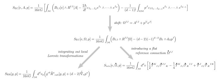
Figure 1: Brief summary of the paper: First of all, we performed a change of variables going from the spin connection to a shifted connection $\Omega$. The new connection $\Omega$ depends on a boundary field $p$, whose norm determines the cosmological constant. Integrating out the internal Lorentz transformations, we obtain a new second-order metric formulation, which resembles unimodular gravity (the norm of $p_{a}$ is determined by the cosmological constant). A non-Abelian version of teleparallel gravity is found by introducing a specific flat reference connection $\accentset{\bullet}{\Omega}$ with $\mathrm{d}_{\accentset{\bullet}{\Omega}}p^{I}=0$.

We would like to emphasize that the change of variables can also be performed when $\Lambda=0$. In this case, $p$ will be a null vector in the Lorentzian case. In the Euclidean case, we can use a Grassmanian number $\theta$ to parametrize $p$ such that $\theta^{2}=0$.

We identified the two associated second-order theories, namely the metric and the teleparallel formulations, see the figure above. The metric formalism associated to the new variables can be seen as a new version of the Henneaux-Teitelboim model for unimodular gravity. We note that the first-order action (60) can also be interpreted as a first-order formulation for unimodular gravity, since it can be supplemented with the normalizing constraint of the vector $p$,

$$S_{\text{EC}}[e,\Omega,p] = \frac{1}{16\pi G}\int_{\mathcal{M}}\Big{(}\Big{(}\frac{1}{(d-2)!}\,\varepsilon_{IJK_{1}\cdots K_{d-2}}\,e^{K_{1}}\wedge\cdots\wedge e^{K_{d-2}}\Big{)}\wedge R^{IJ}[\Omega]$$ (95)

$$-\frac{(d-2)(-1)^{d-2}}{(d-1)!}\Big{(}\varepsilon_{IK_{1}\dots K_{d-1}}e^{K_{1}}\wedge\dots e^{K_{d-1}}\Big{)}\wedge\mathrm{d}_{\Omega}p^{I}-\frac{1}{2}g_{ab}p^{a}p^{b}\,\mathrm{d}\tau\Big{)}\,$$

As in the metric formulation, variation with respect to $\tau$ leads to the norm of $p$ being constant, hence recovering the cosmological constant as a constant of integration. The teleparallel formulation, on the other hand, is now expressed in terms of a non-Abelian field strength (85) that enters the action quadratically (93). With respect to the usual Abelian teleparallel formulation, the Abelian Lie algebra $\mathbb{R}^{d}$ is deformed into the non-abelian Lie algebra $\mathfrak{an}_{d-1}$.

The results of this paper summarized in Fig. 1 opens a number of interesting new directions to explore. The boundary volume term plays an important role in the holographic renormalization context Bianchi:2001kw . It would be interesting to see whether the formulation using the new variables can also be useful, in particular, its connection with unimodular gravity.

The boundary term is the key to understand why quantum groups appear in three dimensions Dupuis:2020ndx . In the four-dimensional context it has been conjectured that they should also be relevant Smolin:2002sz ; Fairbairn:2010cp ; Han:2010pz . It would then be important to study how the charge algebra is affected by adding this term to the theory. In particular, in the list of works Freidel:2020xyx ; Freidel:2020svx ; Freidel:2020ayo , it was always assumed that $\Lambda=0$. It would be worthwhile to study how these results are affected if $\Lambda\neq 0$ and the boundary volume term is also considered.

The non-Abelian formulation of teleparallel gravity is likely to be the classical continuum counterpart of the (deformed) dual BF vacuum Dittrich:2016typ . It would be interesting to construct the discrete picture, which leads upon quantization to such a deformed dual BF vacuum, generalizing Delcamp:2018sef ; Dupuis:2019unm . This is work in progress.

The origin of this work came from studying three-dimensional gravity. Recently, a most general bulk action for three-dimensional gravity was introduced Geiller:2020edh . It would be interesting to see how the change of variables could be of use there, either for discretizing or in recovering the different second order formalisms.

Finally, the canonical transformation is implemented for a constant homogenous curvature, parametrized by the cosmological constant. One might wonder whether we could generalize the construction in the case of a varying curvature. We leave this intriguing question for later investigations.

References

• (1) M. Dupuis, L. Freidel, F. Girelli, A. Osumanu, and J. Rennert, “On the origin of the quantum group symmetry in 3d quantum gravity,” arXiv:2006.10105.
• (2) L. Freidel, K. Krasnov, and R. Puzio, “BF description of higher dimensional gravity theories,” Adv. Theor. Math. Phys. 3 (1999) 1289–1324, arXiv:hep-th/9901069.
• (3) L. Freidel and A. Perez, “Quantum gravity at the corner,” Universe 4 (2018), no. 10, 107, arXiv:1507.02573.
• (4) L. Freidel, M. Geiller, and D. Pranzetti, “Edge modes of gravity. Part I. Corner potentials and charges,” JHEP 11 (2020) 026, arXiv:2006.12527.
• (5) L. Freidel, M. Geiller, and D. Pranzetti, “Edge modes of gravity. Part II. Corner metric and Lorentz charges,” JHEP 11 (2020) 027, arXiv:2007.03563.
• (6) L. Freidel, M. Geiller, and D. Pranzetti, “Edge modes of gravity - III: Corner simplicity constraints,” arXiv:2007.12635.
• (7) E. De Paoli and S. Speziale, “A gauge-invariant symplectic potential for tetrad general relativity,” JHEP 07 (2018) 040, arXiv:1804.09685.
• (8) R. Oliveri and S. Speziale, “Boundary effects in General Relativity with tetrad variables,” arXiv:1912.01016.
• (9) W. Wieland, “Null infinity as an open Hamiltonian system,” arXiv:2012.01889.
• (10) W. Wieland, “New boundary variables for classical and quantum gravity on a null surface,” Class. Quantum Grav. 34 (2017) 215008, arXiv:1704.07391.
• (11) W. Wieland, “Fock representation of gravitational boundary modes and the discreteness of the area spectrum,” Ann. Henri Poincaré 18 (2017) 3695–3717, arXiv:1706.00479.
• (12) W. Wieland, “Conformal boundary conditions, loop gravity and the continuum,” JHEP 10 (2018) 089, arXiv:1804.08643.
• (13) R. Arnowitt, S. Deser, and C. Misner, The dynamics of general relativity, ch. 7, pp. 227–264. Wiley, New York, 1962. arXiv:gr-qc/0405109v1.
• (14) C. Kiefer, Quantum Gravity. Cambridge University Press, Cambridge, 2005.
• (15) C. Thiemann, Introduction to Modern Canonical Quantum General Relativity. Cambridge University Press, 2007.
• (16) A. Ashtekar, “New Variables for Classical and Quantum Gravity,” Phys. Rev. Lett. 57 (1986) 2244–2247.
• (17) J. F. Barbero G., “Real Ashtekar variables for Lorentzian signature space times,” Phys. Rev. D 51 (1995) 5507–5510, arXiv:gr-qc/9410014.
• (18) S. Holst, “Barbero’s Hamiltonian derived from a generalized Hilbert-Palatini action,” Phys. Rev. D 53 (May, 1996) 5966–5969.
• (19) V. V. Fock and A. A. Rosly, “Poisson structure on moduli of flat connections on Riemann surfaces and r matrix,” Am. Math. Soc. Transl. 191 (1999) 67–86, arXiv:math/9802054.
• (20) V. G. Turaev and O. Y. Viro, “State sum invariants of 3-manifolds and quantum 6j-symbols,” Topology 31 (1992), no. 4, 865–902.
• (21) L. Smolin, “Quantum gravity with a positive cosmological constant,” arXiv:hep-th/0209079.
• (22) W. J. Fairbairn and C. Meusburger, “Quantum deformation of two four-dimensional spin foam models,” J. Math. Phys. 53 (2012) 022501, arXiv:1012.4784.
• (23) M. Han, “4-dimensional Spin-foam Model with Quantum Lorentz Group,” J.Math.Phys. 52 (2011) 072501, arXiv:1012.4216.
• (24) M. Henneaux and C. Teitelboim, “The Cosmological Constant and General Covariance,” Phys. Lett. B 222 (1989) 195–199.
• (25) R. Aldrovandi and J. G. Pereira, Teleparallel Gravity, vol. 173 of Fundamental Theories of Physics. Springer-Verlag, 2013.
• (26) M. Bianchi, D. Z. Freedman, and K. Skenderis, “Holographic renormalization,” Nucl. Phys. B 631 (2002) 159–194, arXiv:hep-th/0112119.
• (27) K. Skenderis, “Lecture notes on holographic renormalization,” Class. Quant. Grav. 19 (2002) 5849–5876, arXiv:hep-th/0209067.
• (28) S. MacDowell and F. Mansouri, “Unified Geometric Theory of Gravity and Supergravity,” Phys. Rev. Lett. 38 (1977) 739. [Erratum: Phys.Rev.Lett. 38, 1376 (1977)].
• (29) S. Majid, Foundations of quantum group theory. Cambridge University Press, 2011.
• (30) J. B. Jiménez, L. Heisenberg, and T. S. Koivisto, “The Geometrical Trinity of Gravity,” Universe 5 (2019), no. 7, 173, arXiv:1903.06830.
• (31) B. Dittrich and M. Geiller, “Quantum gravity kinematics from extended TQFTs,” New J. Phys. 19 (2017), no. 1, 013003, arXiv:1604.05195.
• (32) C. Delcamp, L. Freidel, and F. Girelli, “Dual loop quantizations of 3d gravity,” arXiv:1803.03246.
• (33) M. Dupuis, F. Girelli, A. Osumanu, and W. Wieland, “First-order formulation of teleparallel gravity and dual loop gravity,” Class. Quant. Grav. 37 (2020), no. 8, 085023, arXiv:1906.02801.
• (34) M. Geiller, C. Goeller, and N. Merino, “Most general theory of 3d gravity: Covariant phase space, dual diffeomorphisms, and more,” arXiv:2011.09873.