X-CAL: Explicit Calibration for Survival Analysis

Abstract

Survival analysis models the distribution of time until an event of interest, such as discharge from the hospital or admission to the ICU. When a model’s predicted number of events within any time interval is similar to the observed number, it is called well-calibrated. A survival model’s calibration can be measured using, for instance, distributional calibration (d-calibration) (Haider et al., 2020) which computes the squared difference between the observed and predicted number of events within different time intervals. Classically, calibration is addressed in post-training analysis. We develop explicit calibration (x-cal), which turns d-calibration into a differentiable objective that can be used in survival modeling alongside maximum likelihood estimation and other objectives. X-cal allows practitioners to directly optimize calibration and strike a desired balance between predictive power and calibration. In our experiments, we fit a variety of shallow and deep models on simulated data, a survival dataset based on mnist, on length-of-stay prediction using mimic-iii data, and on brain cancer data from The Cancer Genome Atlas. We show that the models we study can be miscalibrated. We give experimental evidence on these datasets that x-cal improves d-calibration without a large decrease in concordance or likelihood.

1 Introduction

A core challenge in healthcare is to assess the risk of events such as onset of disease or death. Given a patient’s vitals and lab values, physicians should know whether the patient is at risk for transfer to a higher level of care. Accurate estimates of the time-until-event help physicians assess risk and accordingly prescribe treatment strategies: doctors match aggressiveness of treatment against severity of illness. These predictions are important to the health of the individual patient and to the allocation of resources in the healthcare system, affecting all patients.

Survival Analysis formalizes this risk assessment by estimating the conditional distribution of the time-until-event for an outcome of interest, called the failure time. Unlike supervised learning, survival analysis must handle datapoints that are censored: their failure time is not observed, but bounds on the failure time are. For example, in a 10 year cardiac health study (Wilson et al., 1998; Vasan et al., 2008), some individuals will remain healthy over the study duration. Censored points are informative, as we can learn that someone’s physiology indicates they are healthy-enough to avoid onset of cardiac issues within the next 10 years.

A well-calibrated survival model is one where the predicted number of events within any time interval is similar to the observed number (Pepe and Janes, 2013). When this is the case, event probabilities can be interpreted as risk and can be used for downstream tasks, treatment strategy, and human-computable risk score development (Sullivan et al., 2004; Demler et al., 2015; Haider et al., 2020). Calibrated conditional models enable accurate, individualized prognosis and may help prevent giving patients misinformed limits on their survival, such as 6 months when they would survive years. Poorly calibrated predictions of time-to-event can misinform decisions about a patient’s future.

Calibration is a concern in today’s deep models. Classical neural networks that were not wide or deep by modern standards were found to be as calibrated as other models after the latter were calibrated (boosted trees, random forests, and svms calibrated using Platt scaling and isotonic regression) (Niculescu-Mizil and Caruana, 2005). However, deeper and wider models using batchnorm and dropout have been found to be overconfident or otherwise miscalibrated (Guo et al., 2017). Common shallow survival models such as the Weibull Accelerated Failure Times (aft) model may also be miscalibrated (Haider et al., 2020). We explore shallow and deep models in this work.

Calibration checks are usually performed post-training. This approach decouples the search for a good predictive model and a well-calibrated one (Song et al., 2019; Platt, 1999; Zadrozny and Elkan, 2002). Recent approaches tackle calibration in-training via alternate loss functions. However, these may not, even implicitly, optimize a well-defined calibration measure, nor do they allow for explicit balance between prediction and calibration (Avati et al., 2019). Calibration during training has been explored recently for binary classification (Kumar et al., 2018). Limited evaluations of calibration in survival models can be done by considering only particular time points: this model is well-calibrated for half-year predictions. Recent work considers d-calibration (Haider et al., 2020), a holistic measure of calibration of time-until-event that measures calibration of distributions.

In this work, we propose to improve calibration by augmenting traditional objectives for survival modeling with a differentiable approximation of d-calibration, which we call explicit calibration (x-cal). X-cal is a plug-in objective that reduces obtaining good calibration to an optimization problem amenable to data sub-sampling. X-cal helps build well-calibrated versions of many existing models and controls calibration during training. In our experiments , we fit a variety of shallow and deep models on simulated data, a survival dataset based on mnist, on length-of-stay prediction using mimic-iii data, and on brain cancer data from The Cancer Genome Atlas. We show that the models we study can be miscalibrated. We give experimental evidence on these datasets that x-cal improves d-calibration without a large decrease in concordance or likelihood.

2 Defining and Evaluating Calibration in Survival Analysis

Survival analysis models the time $\boldsymbol{\mathbf{t}}>0$ until an event, called the failure time. $\boldsymbol{\mathbf{t}}$ is often assumed to be conditionally distributed given covariates $\boldsymbol{\mathbf{x}}$. Unlike typical regression problems, there may also be censoring times $\boldsymbol{\mathbf{c}}$ that determine whether $\boldsymbol{\mathbf{t}}$ is observed. We focus on right-censoring in this work, with observations $(u,\delta,x)$ where $\boldsymbol{\mathbf{u}}=\min(\boldsymbol{\mathbf{t}},\boldsymbol{\mathbf{c}})$ and $\boldsymbol{\delta}=\mathbbm{1}\left[\boldsymbol{\mathbf{t}}<\boldsymbol{\mathbf{c}}\right]$. If $\delta=1$ then $u$ is a failure time. Otherwise $u$ is a censoring time and the datapoint is called censored. Censoring times may be constant or random. We assume censoring-at-random: $\boldsymbol{\mathbf{t}}\mathchoice{\mathrel{\hbox to0.0pt{$\displaystyle\perp$\hss}\mkern 2.0mu{\displaystyle\perp}}}{\mathrel{\hbox to0.0pt{$\textstyle\perp$\hss}\mkern 2.0mu{\textstyle\perp}}}{\mathrel{\hbox to0.0pt{$\scriptstyle\perp$\hss}\mkern 2.0mu{\scriptstyle\perp}}}{\mathrel{\hbox to0.0pt{$\scriptscriptstyle\perp$\hss}\mkern 2.0mu{\scriptscriptstyle\perp}}}\boldsymbol{\mathbf{c}}~{}|~{}\boldsymbol{\mathbf{x}}$.

We denote the joint distribution of $(\boldsymbol{\mathbf{t}},\boldsymbol{\mathbf{x}})$ by $P$ and the conditional cumulative distribution function (cdf) of $\boldsymbol{\mathbf{t}}~{}|~{}\boldsymbol{\mathbf{x}}$ by $F$ (sometimes denoting the marginal cdf by $F$ when clear). Whenever distributions or cdfs have no subscript parameters, they are taken to be true data-generating distributions and when they have parameters $\theta$ they denote a model. We give more review of key concepts, definitions, and common survival analysis models in Appendix A.

2.1 Defining Calibration

We first establish a common definition of calibration for binary outcome. Let $\boldsymbol{\mathbf{x}}$ be covariates and let $\boldsymbol{\mathbf{d}}$ be a binary outcome distributed conditional on $\boldsymbol{\mathbf{x}}$. Let them have joint distribution $P(\boldsymbol{\mathbf{d}},\boldsymbol{\mathbf{x}})$. Define $\mathtt{risk}_{\theta}(x)$ as the modeled probability $P_{\theta}(\boldsymbol{\mathbf{d}}=1~{}|~{}x)$, a deterministic function of $x$. Pepe and Janes (2013) define calibration as the condition that

$$\mathbb{P}(\boldsymbol{\mathbf{d}}=1~{}|~{}\mathtt{risk}_{\theta}(\boldsymbol{\mathbf{x}})=r)=\approx r.$$ (1)

That is, the frequency of events is $r$ among subjects whose modeled risks are equal to $r$. For a survival problem with joint distribution $P(\boldsymbol{\mathbf{t}},\boldsymbol{\mathbf{x}})$, we can define risk to depend on an observed failure time instead of the binary outcome $\boldsymbol{\mathbf{d}}=1$. With $F_{\theta}$ as the model cdf, the definition of risk for survival analysis becomes $\mathtt{risk}_{\theta}(t,x)=F_{\theta}(t~{}|~{}x)$, a deterministic function of $(t,x)$. Then perfect calibration is the condition that, for all sub-intervals $I=[a,b]$ of $[0,1]$,

$$\mathbb{P}(\mathtt{risk}_{\theta}(\boldsymbol{\mathbf{t}},\boldsymbol{\mathbf{x}})\in I)=\mathop{\mathbb{E}}_{P(\boldsymbol{\mathbf{t}},\boldsymbol{\mathbf{x}})}\mathbbm{1}\left[F_{\theta}(\boldsymbol{\mathbf{t}}~{}|~{}\boldsymbol{\mathbf{x}})\in I\right]=|I|.$$ (2)

This is because, for continuous $F$ (an assumption we keep for the remainder of the text), cdfs transform samples of their own distribution to $\text{Unif}(0,1)$ variates. Thus, when model predictions are perfect and $F_{\theta}=F$, the probability that $F_{\theta}(\boldsymbol{\mathbf{t}}~{}|~{}\boldsymbol{\mathbf{x}})$ takes a value in interval $I$ is equal to $|I|$. Since the expectation is taken over $\boldsymbol{\mathbf{x}}$, the same holds when $F_{\theta}(t~{}|~{}x)=F(t)$, the true marginal cdf.

2.2 Evaluating Calibration

Classical tests and their recent modifications assess calibration of survival models for a particular time of interest $t^{*}$ by comparing observed versus modeled event frequencies (Lemeshow and Hosmer Jr, 1982; Gronnesby and Borgan, 1996; D’agostino and Nam, 2003; Royston and Altman, 2013; Demler et al., 2015; Yadlowsky et al., 2019). They apply the condition in Equation 1 for the classification task $\boldsymbol{\mathbf{t}}<t^{*}~{}|~{}\boldsymbol{\mathbf{x}}$. These tests are limited in two ways 1) it is not clear how to combine calibration assessments over the entire range of possible time predictions (Haider et al., 2020) and 2) they answer calibration in a rigid yes/no fashion with hypothesis testing. We briefly review these tests in Appendix A.

D-calibration

Haider et al. (2020) develop distributional calibration (d-calibration) to test the calibration of conditional survival distributions across all times. D-calibration uses the condition in Equation 2 and checks the extent to which it holds by evaluating the model conditional cdf on times in the data and checking that these cdf evaluations are uniform over $[0,1]$. This uniformity ensures that observed and predicted numbers of events within each time interval match.

To set this up formally, recall that $F$ denotes the unknown true cdf. For each individual $x$, let $F_{\theta}(\boldsymbol{\mathbf{t}}~{}|~{}x)$ denote the modeled cdf of time-until-failure. To measure overall calibration error, d-calibration accumulates the squared errors of the equality condition in Equation 2 over sets $I\in\mathcal{I}$ that cover $[0,1]$:

$$\mathcal{R}(\theta):=\sum_{I\in\mathcal{I}}\left(\mathop{\mathbb{E}}_{P(\boldsymbol{\mathbf{t}},\boldsymbol{\mathbf{x}})}\mathbbm{1}\left[F_{\theta}(\boldsymbol{\mathbf{t}}~{}|~{}\boldsymbol{\mathbf{x}})\in I\right]-|I|\right)^{2}.$$ (3)

The collection $\mathcal{I}$ is chosen to contain disjoint contiguous intervals $I\subseteq[0,1]$, that cover the whole interval $[0,1]$. Haider et al. (2020) perform a $\chi^{2}$-test to determine whether a model is well-calibrated, replacing the expectation in Equation 3 with a Monte Carlo estimate.

Properties

Setting aside the hypothesis testing step, we highlight two key properties of d-calibration. First, d-calibration is zero for the correct conditional model. This ensures that the correct model is not wrongly mischaracterized as miscalibrated. Second, for a given model class and dataset, smaller d-calibration means a model is more calibrated. This means that it makes sense to minimize d-calibration. Next, we make use of these properties and turn d-calibration into a differentiable objective.

3 X-cal: A Differentiable Calibration Objective

We measure calibration error with d-calibration (Equation 3) and propose to incorporate it into our training and minimize it directly. However, the indicator function $\mathbbm{1}\left[\cdot\right]$ poses a challenge for optimization. Instead, we derive a soft version of d-calibration using a soft set membership function. We then develop an upper-bound to soft d-calibration that we call x-cal that supports subsampling for stochastic optimization with batch data.

3.1 Soft Membership d-calibration

We replace the membership indicator for a set $I$ with a differentiable function. Let $\gamma>0$ be a temperature parameter. Let $\sigma(x)=(1+\exp[-x])^{-1}$. For point $u$ and the set $I=[a,b]$, define soft membership $\zeta_{\gamma}$ as

$$\zeta_{\gamma}(u;I):=\sigma(\gamma(u-a)(b-u)),$$ (4)

where $\gamma\rightarrow\infty$ makes membership exact. This is visualized in Figure 2 in Appendix G. We propose the following differentiable approximation to Equation 3, which we call soft d-calibration, for use in a calibration objective:

$$\hat{\mathcal{R}}_{\gamma}(\theta):=\sum_{I\in\mathcal{I}}\left(\mathop{\mathbb{E}}_{P(\boldsymbol{\mathbf{t}},\boldsymbol{\mathbf{x}})}\zeta_{\gamma}\left(F_{\theta}(\boldsymbol{\mathbf{t}}~{}|~{}\boldsymbol{\mathbf{x}});I\right)-|I|\right)^{2}.$$ (5)

We find that $\gamma=10^{4}$ allows for close-enough approximation to optimize exact d-calibration.

3.2 Stochastic Optimization via Jensen’s Inequality

Soft d-calibration squares an expectation over the data, meaning that its gradient includes a product of two expectations over the same data. Due to this, it is hard to obtain a low-variance, unbiased gradient estimate with batches of data, which is important for models that rely on stochastic optimization. To remedy this, we develop an upper-bound on soft d-calibration, which we call x-cal, whose gradient has an easier unbiased estimator.

Let $R_{\gamma,\theta}(t,x,I)$ denote the contribution to soft d-calibration error due to one set $I$ and a single sample $(t,x)$ in Equation 5: $R_{\gamma,\theta}(t,x,I):=\zeta_{\gamma}\left(F_{\theta}(t~{}|~{}x);I\right)-|I|$. Then soft d-calibration can be written as:

$$\hat{\mathcal{R}}_{\gamma}(\theta)=\sum_{I\in\mathcal{I}}\left(\mathop{\mathbb{E}}_{P(\boldsymbol{\mathbf{t}},\boldsymbol{\mathbf{x}})}R_{\gamma,\theta}(\boldsymbol{\mathbf{t}},\boldsymbol{\mathbf{x}},I)\right)^{2}.$$

For each term in the sum over sets $I$, we proceed by in two steps. First, replace the expectation over data $\mathop{\mathbb{E}}_{P}$ with an expectation over sets of samples $\mathop{\mathbb{E}}_{S\sim P^{M}}$ of the mean of $R_{\gamma,\theta}$ where $S$ is a set of size $M$. Second, use Jensen’s inequality to switch the expectation and square.

$$\begin{split}\hat{\mathcal{R}}_{\gamma}(\theta)=\sum_{I\in\mathcal{I}}\left(\mathop{\mathbb{E}}_{S\sim P^{M}}\frac{1}{M}\sum_{t,x\in S}R_{\gamma,\theta}(t,x,I)\right)^{2}\leq\mathop{\mathbb{E}}_{S\sim P^{M}}\sum_{I\in\mathcal{I}}\left(\frac{1}{M}\sum_{t,x\in S}R_{\gamma,\theta}(t,x,I)\right)^{2}.\end{split}$$ (6)

We call this upper-bound x-cal and denote it by $\hat{\mathcal{R}}_{\gamma}^{+}(\theta)$. To summarize, $\lim_{\gamma\rightarrow\infty}\hat{\mathcal{R}}_{\gamma}(\theta)=\mathcal{R}(\theta)$ by soft indicator approximation and $\hat{\mathcal{R}}_{\gamma}(\theta)\leq\hat{\mathcal{R}}_{\gamma}^{+}(\theta)$ by Jensen’s inequality. As $M\rightarrow\infty$, the slack introduced due to Jensen’s inequality vanishes (in practice we are constrained by the size of the dataset). We now derive the gradient with respect to $\theta$, using $\zeta^{\prime}(u)=\frac{d\zeta}{du}(u)$:

$$\frac{d\hat{\mathcal{R}}_{\gamma}^{+}}{d\theta}=\mathop{\mathbb{E}}_{S\sim P^{M}}\sum_{I\in\mathcal{I}}\frac{2}{M^{2}}\sum_{t,x\in S}R_{\gamma,\theta}(t,x,I)\left(\zeta_{\gamma}^{\prime}\left({F_{\theta}}(t~{}|~{}x);I\right)\frac{dF_{\theta}}{d\theta}(t~{}|~{}x)\right).$$ (7)

We estimate Equation 7 by sampling batches $S$ of size $M$ from the empirical data.

Analyzing this gradient demonstrates how x-cal works. If the fraction of points in bin $I$ is larger than $|I|$, x-cal pushes points out of $I$. The gradient of $\zeta_{\gamma}$ pushes points in the first half of the bin to have smaller cdf values and similarly points in the second half are pushed upwards.

While this works well for intervals not at the boundary of $[0,1]$, some care must be taken at the boundaries. cdf values in the last bin may be pushed to one and unable to leave the bin. Since the maximum cdf value is one, $\mathbbm{1}\left[u\in[a,1]\right]=\mathbbm{1}\left[u\in[a,b]\right]$ for any $b>1$. Making use of this property, x-cal extends the right endpoint of the last bin so that all cdf values are in the first half of the bin and therefore are pushed to be smaller. The boundary condition near zero is similar. We provide further analysis in Appendix I.

x-cal can be added to loss functions such as negative log likelihood (nll) and other survival modeling objectives such as Survival-crps (crps) (Avati et al., 2019). For example, the full x-calibrated maximum likelihood objective for a model $P_{\theta}$ and $\lambda>0$ is:

$$\min_{\theta}\mathop{\mathbb{E}}_{P(\boldsymbol{\mathbf{t}},\boldsymbol{\mathbf{x}})}-\log P_{\theta}(\boldsymbol{\mathbf{t}}~{}|~{}\boldsymbol{\mathbf{x}})+\lambda\hat{\mathcal{R}}_{\gamma}^{+}(\theta).$$ (8)

Choosing $\gamma$

For small $\gamma$, soft d-calibration is a poor approximation to d-calibration. For large $\gamma$, gradients vanish, making it hard to optimize d-calibration. We find that setting $\gamma=10000$ worked in all experiments. We evaluate the choice of $\gamma$ in Appendix G.

Bound Tightness

The slack in Jensen’s inequality does not adversely affect our experiments in practice. We successfully use small batches, e.g. $<1000$, for datasets such as mnist. We always report exact d-calibration in the results. We evaluate the tightness of this bound and show that models ordered by the upper-bound are ordered in d-calibration the same way in Appendix H.

3.3 Handling Censored Data

In presence of right-censoring, failure times are censored more often than earlier times. So, applying the true cdf to only uncensored failure times results in a non-uniform distribution skewed to smaller values in $[0,1]$. Censoring must be taken into account.

Let $x$ be a censored point with observed censoring time $u$ and unobserved failure time $\boldsymbol{\mathbf{t}}$. Recall that $\boldsymbol{\delta}=\mathbbm{1}\left[\boldsymbol{\mathbf{t}}<\boldsymbol{\mathbf{c}}\right]$. In this case $\boldsymbol{\mathbf{c}}=\boldsymbol{\mathbf{u}}=u$ and $\boldsymbol{\delta}=0$. Let $F_{\boldsymbol{\mathbf{t}}}=F(\boldsymbol{\mathbf{t}}~{}|~{}x)$, $F_{\boldsymbol{\mathbf{c}}}=F(\boldsymbol{\mathbf{c}}~{}|~{}x)$, and $F_{\boldsymbol{\mathbf{u}}}=F(\boldsymbol{\mathbf{u}}~{}|~{}x)$. We first state the fact that, under $\boldsymbol{\mathbf{t}}\mathchoice{\mathrel{\hbox to0.0pt{$\displaystyle\perp$\hss}\mkern 2.0mu{\displaystyle\perp}}}{\mathrel{\hbox to0.0pt{$\textstyle\perp$\hss}\mkern 2.0mu{\textstyle\perp}}}{\mathrel{\hbox to0.0pt{$\scriptstyle\perp$\hss}\mkern 2.0mu{\scriptstyle\perp}}}{\mathrel{\hbox to0.0pt{$\scriptscriptstyle\perp$\hss}\mkern 2.0mu{\scriptscriptstyle\perp}}}\boldsymbol{\mathbf{c}}~{}|~{}\boldsymbol{\mathbf{x}}$, a datapoint observed to be censored at time $u$ has $F_{\boldsymbol{\mathbf{t}}}\sim\text{Unif}(F_{u},1)$ for true cdf $F$ (proof in Appendix C). This means that we can compute the probabilty that $\boldsymbol{\mathbf{t}}$ falls in each bin $I=[a,b]$:

$$\mathbb{P}(F_{\boldsymbol{\mathbf{t}}}\in I~{}|~{}\delta=0,u,x)=\frac{(b-F_{u})\mathbbm{1}\left[F_{u}\in I\right]}{1-F_{u}}+\frac{(b-a)\mathbbm{1}\left[F_{u}<a\right]}{1-F_{u}},$$ (9)

Haider et al. (2020) make this observation and suggest a method for handling censoring points: they contribute $\mathbb{P}(F_{\boldsymbol{\mathbf{t}}}\in I~{}|~{}\delta=0,u,x)$ in place of the unobserved $\mathbbm{1}\left[F_{\boldsymbol{\mathbf{t}}}\in I\right]$:

$$\sum_{I\in\mathcal{I}}\Big{(}\mathop{\mathbb{E}}_{\boldsymbol{\mathbf{u}},\boldsymbol{\delta},\boldsymbol{\mathbf{x}}}\Big{[}\boldsymbol{\delta}\mathbbm{1}\left[F_{\boldsymbol{\mathbf{u}}}\in I\right]+(1-\boldsymbol{\delta})\mathbb{P}(F_{\boldsymbol{\mathbf{t}}}\in I~{}|~{}\boldsymbol{\delta},\boldsymbol{\mathbf{u}},\boldsymbol{\mathbf{x}})\Big{]}-|I|\Big{)}^{2}.$$ (10)

This estimator does not change the expectation defining d-calibration, thereby preserving the property that d-calibration is $0$ for a calibrated model. We soften Equation 9 with:

$$\zeta_{\gamma,cens}(F_{u};I):=\frac{(b-F_{u})\sigma(\gamma(F_{u}-a)(b-F_{u}))}{(1-F_{u})}+\frac{(b-a)\sigma(\gamma(a-F_{u}))}{(1-F_{u})},$$

where we have used a one-sided soft indicator for $\mathbbm{1}\left[F_{u}<a\right]$ in the right-hand term. We use $\zeta_{\gamma,cens}$ in place of $\zeta_{\gamma}$ for censored points in soft d-calibration. This gives the following estimator for soft d-calibration with censoring:

$$\sum_{I\in\mathcal{I}}\Big{(}\mathop{\mathbb{E}}_{\boldsymbol{\mathbf{u}},\boldsymbol{\delta},\boldsymbol{\mathbf{x}}}\Big{[}\boldsymbol{\delta}\zeta_{\gamma}(F_{\theta}(\boldsymbol{\mathbf{u}}~{}|~{}\boldsymbol{\mathbf{x}});I)+(1-\boldsymbol{\delta})\zeta_{\gamma,cens}(F_{\theta}(\boldsymbol{\mathbf{u}}~{}|~{}\boldsymbol{\mathbf{x}});I)\Big{]}-|I|\Big{)}^{2}.$$ (11)

The upper-bound of Equation 11 and its corresponding gradient can be derived analogously to the uncensored case. We use these in ours experiments on censored data.

4 Experiments

We study how x-cal allows the modeler to optimize for a specified balance between prediction and calibration. We augment maximum likelihood estimation with x-cal for various settings of coefficient $\lambda$, where $\lambda=0$ corresponds to vanilla maximum likelihood. Maximum likelihood for survival analysis is described in Appendix A (Equation 12). For the log-normal experiments, we also use Survival-crps (crps) (Avati et al., 2019) with x-cal since s-crps enjoys a closed-form for log-normal. S-crps was developed to produce calibrated survival models but it optimizes neither a calibration measure nor a traditional likelihood. See Appendix B for a description of s-crps.

Models, Optimization, and Evaluation

We use log-normal, Weibull, Categorical and Multi-Task Logistic Regression (mtlr) models with various linear or deep parameterizations. For the discrete models, we optionally interpolate their cdf (denoted in the tables by ni for not-interpolated and i for interpolated). See Appendix E for general model descriptions. Experiment-specific model details may be found in Appendix F. We use $\gamma=10000$. We use $20$ d-calibration bins disjoint over $[0,1]$ for all experiments except for the cancer data, where we use $10$ bins as in Haider et al. (2020). For all experiments, we measure the loss on a validation set at each training epoch to chose a model to report test set metrics with. We report the test set nll, test set d-calibration and Harrell’s Concordance Index (Harrell Jr et al., 1996) (abbreviated conc) on the test set for several settings of $\lambda$. We compute concordance using the Lifelines package (Davidson-Pilon et al., 2017). All reported results are an average of three seeds.

Data

We discuss differences in performance on simulated gamma data, semi-synthetic survival data where times are conditional on the mnist classes, length of stay prediction in the Medical Information Mart for Intensive Care (mimic-iii) dataset (Johnson et al., 2016), and glioma brain cancer data from The Cancer Genome Atlas (tcga). Additional data details may be found in Appendix D.

4.1 Experiment 1: Simulated Gamma Times with Log-Linear Mean

Data

We design a simulation study to show that a conditional distribution may achieve good concordance and likelihood but will have poor d-calibration. After adding x-cal, we are able to improve the exact d-calibration. We sample $\boldsymbol{\mathbf{x}}\in\mathbb{R}^{32}$ from a multivariate normal with $\sigma^{2}=10.0$. We sample times $\boldsymbol{\mathbf{t}}$ conditionally from a gamma with mean $\boldsymbol{\mathbf{\mu}}$ that is log-linear in $\boldsymbol{\mathbf{x}}$ and constant variance 1e-3. The censoring times $\boldsymbol{\mathbf{c}}$ are drawn like the event times, except with a different coefficient for the log-linear function. We experiment with censored and uncensored simulations, where we discard $\boldsymbol{\mathbf{c}}$ and always observe $\boldsymbol{\mathbf{t}}$ for uncensored. We sample a train/validation/test sets with 100k/50k/50k datapoints, respectively.

Results

Due to high variance in $\boldsymbol{\mathbf{x}}$ and low conditional variance, this simulation has low noise. With large, clean data, this experiment validates the basic method on continuous and discrete models in the presence of censoring. Table 1 demonstrates how increasing $\lambda$ gracefully balances d-calibration with nll and concordance for different models and objectives: log-normal trained via nll and with s-crps, and the categorical model trained via nll, without cdf interpolation. For results on more models and choices of $\lambda$ see Table 9 for uncensored results and Table 10 for censored in Appendix J.

Table 1: Gamma simulation, censored

	$\lambda$	0	1	10	100	500	1000
Log-Norm	nll	-0.059	-0.049	0.004	0.138	0.191	0.215
nll	d-cal	0.029	0.020	0.005	2e-4	6e-5	7e-5
	conc	0.981	0.969	0.942	0.916	0.914	0.897
Log-Norm	nll	0.038	0.084	0.143	0.201	0.343	0.436
s-crps	d-cal	0.017	0.007	0.001	1e-4	5e-5	8e-5
	conc	0.982	0.978	0.963	0.950	0.850	0.855
Cat-ni	nll	0.797	0.799	0.822	1.149	1.665	1.920
	d-cal	0.009	0.006	0.002	2e-4	6e-5	6e-5
	conc	0.987	0.987	0.987	0.976	0.922	0.861

4.2 Experiment 2: Semi-Synthetic Experiment: Survival MNIST

Data

Following Polsterl (2019), we simulate a survival dataset conditionally on the mnist dataset (LeCun et al., 2010). Each mnist label gets a deterministic risk score, with labels loosely grouped together by risk groups (Table 5 in Section D.2). Datapoint image $\boldsymbol{\mathbf{x}}_{i}$ with label $\boldsymbol{\mathbf{y}}_{i}$ has time $\boldsymbol{\mathbf{t}}_{i}$ drawn from a Gamma with mean equal to $\text{risk}(y_{i})$ and constant variance 1e-3. Therefore $\boldsymbol{\mathbf{t}}_{i}\mathchoice{\mathrel{\hbox to0.0pt{$\displaystyle\perp$\hss}\mkern 2.0mu{\displaystyle\perp}}}{\mathrel{\hbox to0.0pt{$\textstyle\perp$\hss}\mkern 2.0mu{\textstyle\perp}}}{\mathrel{\hbox to0.0pt{$\scriptstyle\perp$\hss}\mkern 2.0mu{\scriptstyle\perp}}}{\mathrel{\hbox to0.0pt{$\scriptscriptstyle\perp$\hss}\mkern 2.0mu{\scriptscriptstyle\perp}}}\boldsymbol{\mathbf{x}}_{i}~{}|~{}\boldsymbol{\mathbf{y}}_{i}$ and times for datapoints that share an mnist class are identically drawn. We draw censoring times $\boldsymbol{\mathbf{c}}$ uniformly between the minimum failure time and the $90^{th}$ percentile time, which resulted in about 50% censoring. We use PyTorch’s mnist with test split into validation/test. The model does not see the mnist class and learns a distribution over times given pixels $\boldsymbol{\mathbf{x}}_{i}$. We experiment with censored and uncensored simulations, where we discard $\boldsymbol{\mathbf{c}}$ and always observe $\boldsymbol{\mathbf{t}}$ for uncensored.

Results

This semi-synthetic experiment tests the ability to tune calibration in presence of a high-dimensional conditioning set (mnist images) and through a typical convolutional architecture. Table 2 demonstrates that the deep log-normal models started off miscalibrated relative to the categorical model for $\lambda=0$ and that all models were able to significantly improve in calibration. See Table 11 and Table 12 for more uncensored and censored survival-mnist results.

Table 2: Survival-mnist, censored

	$\lambda$	0	1	10	100	500	1000
Log-Norm	nll	4.337	4.377	4.483	4.682	4.914	5.151
nll	d-cal	0.392	0.074	0.020	0.005	0.005	0.007
	conc	0.902	0.873	0.794	0.696	0.628	0.573
Log-Norm	nll	4.950	4.929	4.859	4.749	4.786	4.877
s-crps	d-cal	0.215	0.122	0.051	0.010	0.002	9e-4
	conc	0.891	0.881	0.874	0.868	0.839	0.815
Cat-ni	nll	1.733	1.734	1.765	1.861	2.074	3.030
	d-cal	0.018	0.014	0.004	5e-4	5e-4	4e-4
	conc	0.945	0.945	0.927	0.919	0.862	0.713

4.3 Experiment 3: Length of Stay Prediction in MIMIC-III

Data

We predict the length of stay (in number of hours) in the ICU, using data from the mimic-iii dataset. Such predictions are important both for individual risk predictions and prognoses and for hospital-wide resource management. We follow the preprocessing in Harutyunyan et al. (2017), a popular mimic-iii benchmarking paper and repository . The covariates are a time series of $17$ physiological variables (Table 6 in Section D.3) including respiratory rate and glascow coma scale information. There is no censoring in this task. We skip imputation and instead use missingness masks as features. There are $2,925,434$ and $525,912$ instances in the training and test sets. We split the training set in half for train and validation.

Results

Harutyunyan et al. (2017) discuss the difficult of this task when predicting fine-grained lengths-of-stay, as opposed to simpler classification tasks like more/less one week stay. The true conditionals are high in entropy given the chosen covariates Table 3 demonstrates this difficulty, as can be seen in the concordances. We report the categorical model with and without cdf interpolation and the log-normal trained with s-crps. Nll for the log-normal is not reported because s-crps does not optimize nll and did poorly on this metric. The log-normal trained with nll was not able to fit this task on any of the three metrics. All three models reported are able to reduce d-calibration. Results for all models and more choices of $\lambda$ may be found in Table 13. The categorical models with and without cdf interpolation match in concordance for $\lambda=0$ and $\lambda=1000$. However, the interpolated model achieves better d-calibration. This may be due to the lower-bound $\ell>0$ on a discrete model’s d-calibration (Appendix E).

Table 3: mimic-iii length of stay

	$\lambda$	0	1	10	100	500	1000
Log-Norm	d-cal	0.859	0.639	0.155	0.046	0.009	0.005
s-crps	conc	0.625	0.639	0.575	0.555	0.528	0.506
Cat-ni	Test nll	3.142	3.177	3.167	3.088	3.448	3.665
	d-cal	0.002	0.002	0.001	2e-4	1e-4	1e-4
	conc	0.702	0.700	0.699	0.690	0.642	0.627
Cat-i	nll	3.142	3.075	3.073	3.073	3.364	3.708
	d-cal	4e-4	2e-4	2e-4	1e-4	5e-5	4e-5
	conc	0.702	0.702	0.702	0.695	0.638	0.627

4.4 Experiment 4: Glioma data from The Cancer Genome Atlas

We use the glioma (a type of brain cancer) dataset collected as part of the tcga program and studied in (Network, 2015). We focus on predicting time until death from the clinical data, which includes tumor tissue location, time of pathological diagnosis, Karnofsky performance score, radiation therapy, demographic information, and more. Censoring means they did not pass away. The train/validation/test sets are made of 552/276/277 datapoints respectively, of which 235/129/126 are censored, respectively.

Results

For this task, we study the Weibull aft model, reduce the deep log-normal model from three to two hidden layers, and study a linear mtlr model (with cdf interpolation) in place of the deep categorical due to the small data size. Mtlr is more constrained than linear categorical due to shared parameters. Table 4 demonstrates these three models’ ability to improve d-calibration. mtlr is able to fit well and does not give up much concordance. Results for all models and more choices of $\lambda$ may be found in Table 14.

Table 4: The Cancer Genome Atlas, glioma

	$\lambda$	0	1	10	100	500	1000
Log-Norm	nll	14.187	6.585	4.639	4.181	4.403	4.510
nll	d-cal	0.059	0.024	0.010	0.003	0.002	0.004
	conc	0.657	0.632	0.703	0.805	0.474	0.387
Weibull	nll	4.436	4.390	4.292	4.498	4.475	4.528
	d-cal	0.035	0.028	0.009	0.003	0.004	0.007
	conc	0.788	0.785	0.777	0.702	0.608	0.575
mtlr-ni	nll	1.624	1.620	1.636	1.658	1.748	1.758
	d-cal	0.009	0.007	0.005	0.003	0.002	0.002
	conc	0.828	0.829	0.824	0.818	0.788	0.763

5 Related Work

Deep Survival Analysis

Recent approaches to survival analysis parameterize the failure distribution as a deep neural network function of the (Ranganath et al., 2016; Alaa and van der Schaar, 2017; Katzman et al., 2018). Miscouridou et al. (2018) and Lee et al. (2018) use a discrete categorical distribution over times interpreted ordinally, which can approximate any smooth density with sufficient data. The categorical approach has also been used when the conditional is parameterized by a recurrent neural network of sequential covariates (Giunchiglia et al., 2018; Ren et al., 2019). Miscouridou et al. (2018) extend deep survival analysis to deal with missingness in $\boldsymbol{\mathbf{x}}$.

Post-training calibration methods

Practitioners have used two calibration methods for binary classifiers, which modify model predictions maximize likelihood on a held-out dataset. Platt scaling (Platt, 1999) works by using a scalar logistic regression built on top of predicted probabilities. Isotonic regression (Zadrozny and Elkan, 2002) uses a nonparametric piecewise linear transformation instead of the logistic regression. These methods do not reveal an explicit balance between prediction quality and calibration during model training. X-cal allows practitioners to explore this balance while searching in the full model space.

Objectives

When an unbounded loss function (e.g. nll) is used and the gradients are a function of $x$, the model may put undue focus on explaining a given outlier $x^{\star}$, worsening calibration during training. For this reason, robust objectives have been explored. Avati et al. (2019) consider continuous ranked probability score (crps) (Matheson and Winkler, 1976), a robust proper scoring rule for continuous outcomes, and adapt it to s-crps for survival analysis by accounting for censoring. However, s-crps does not provide a clear way to balance predictive power and calibration. Kumar et al. (2018) develop a trainable kernel-based calibration measure for binary classification but they do not discuss an optimizable calibration metric for survival analysis.

Brier Score

The Brier Score (Brier and Allen, 1951) decomposes into a calibration metric (numerator of Hosmer-Lemeshow) and a discrimination term encouraging patients with the same failure status at $t^{\star}$ to have the same failure probability at $t^{\star}$. To capture entire distributions over time, the Integrated Brier Score is used. The Inverse Probability of Censoring Weighting Brier Score (Graf et al., 1999) handles censoring but requires estimation of the censoring distribution, a whole survival analysis problem (with censoring due to the failures) on its own (Gerds and Schumacher, 2006; Kvamme and Borgan, 2019). X-cal can balance discrimination and calibration without estimation of the censoring distribution.

6 Discussion

Model calibration is an important consideration in many clinical problems, especially when treatment decisions require risk estimates across all times in the future. We tackle the problem of building models that are calibrated over individual failure distributions. To this end, we provide a new technique that explicitly targets calibration during model training. We achieve this by constructing a differentiable approximation of d-calibration, and using it as an add-on objective to maximum likelihood and s-crps. As we show in our experiments, x-cal allows for explicit and direct control of calibration on both simulated and real data. Further, we showed that searching over the x-cal $\lambda$ parameter can strike the practitioner-specified balance between predictive power and calibration.

Marginal versus Conditional Calibration

d-calibration is $0$ for the true conditional and marginal distributions of failure times. This is because d-calibration measures marginal calibration, i.e. $\boldsymbol{\mathbf{x}}$ is integrated out. Conditional calibration is the stronger condition that $F_{\theta}(t~{}|~{}x)$ is calibrated for all $x$. This is in general infeasible even to measure (let alone optimize) (Vovk et al., 2005; Pepe and Janes, 2013; Barber et al., 2019) without strong assumptions since for continuous $x$ we usually observe just one sample. However, among the distributions that have $0$ d-calibration, the true conditional distribution has the smallest nll. Therefore, x-calibrated objectives with proper scoring rules (like nll) have an optimum only for the true conditional model in the limit of infinite data.

D-Calibration and Censoring

Equation 10 in Section 3.3 provides a censored version of d-calibration that is $0$ for a calibrated model, like the original d-calibration (Equation 3). However, this censored calibration measure is not equal to d-calibration in general for miscalibrated models. For a distribution $F_{\theta}$ with non-zero d-calibration, for any censoring distribution $G$, estimates of the censored version will assess $F_{\theta}$ to be more uniform than if exact d-calibration were able to be computed using all true observed failure times. This happens especially in the case of heavy and early censoring because a lot of uniform weight is assigned (Haider et al., 2020; Avati et al., 2019). This means that the censored objective can be close to $0$ for a miscalibrated model on a highly censored dataset.

An alternative strategy that avoids this issue is to use inverse weighting methods (e.g. Inverse Propensity Estimator of outcome under treatment (Horvitz and Thompson, 1952), Inverse Probability of Censoring-Weighted Brier Score (Graf et al., 1999; Gerds and Schumacher, 2006) and Inverse Probability of Censoring-Weighted binary calibration for survival analysis (Yadlowsky et al., 2019)). Inverse weighting would preserve the expectation that defines d-calibration for any censoring distribution. One option is to adjust with $p(\boldsymbol{\mathbf{c}}~{}|~{}\boldsymbol{\mathbf{x}})$. This requires $\boldsymbol{\mathbf{c}}\perp\boldsymbol{\mathbf{t}}~{}|~{}\boldsymbol{\mathbf{x}}$ and solving an additional censored survival problem $p(\boldsymbol{\mathbf{c}}~{}|~{}\boldsymbol{\mathbf{x}})$. Nevertheless, if a censoring estimate is provided, the methodology in this work could then be applied to an inverse-weighted d-calibration. There is then a trade-off between the censored estimator proposed by Haider et al. (2020) that we use (no modeling $G$) and inverse-weighted estimators (which preserve d-calibration for miscalibrated models).

Broader Impact

In this paper, we study calibration of survival analysis models and suggest an objective for improving calibration during model training. Since calibration means that modeled probabilities correspond to the actual observed risk of an event, practitioners may feel more confident about using model outputs directly for decision making e.g. to decide how many emergency room staff members qualified for performing a given procedure should be present tomorrow given all current ER patients. But if the distribution of event times in these patients differs from validation data, because say the population has different demographics, calibration should not provide the practitioner with more confidence to directly use such model outputs.

Appendix A Background on Survival Analysis and Related Work

Survival analysis models the probability distribution of a time-until-event. The event is often called a failure time. For example, we may model time until onset of coronary heart disease given a patient’s current health status (Wilson et al., 1998; Vasan et al., 2008).

Survival analysis differs from standard probabilistic regression problems in that data may be censored. For example, a patient may leave a study before developing the studied condition, or may not develop the condition before the study ends. In these cases, the time that a patient leaves or the study ends is called the censoring time. These are cases of right-censoring, where it is only known that the failure time is greater than the observed censoring time.

We review key definitions in survival analysis. See George et al. (2014) for a review. For textbooks, see Andersen et al. (2012), Kalbfleisch and Prentice (2002), and Lawless (2011).

A.1 Notation

Let $\boldsymbol{\mathbf{t}}$ be a continuous random variable denoting the failure time with cdf $F$ and density $f$. The survival function $\overline{F}$ is defined as 1 minus the cdf: $\overline{F}=1-F$. Censoring times are considered random variables $\boldsymbol{\mathbf{c}}$ with cdf $G$, survival function $\overline{G}$, and density $g$. In general these distributions may be conditional on covariates $\boldsymbol{\mathbf{x}}$.

For datapoints $i$, let $\boldsymbol{\mathbf{t}}_{i}$ be failure times and $\boldsymbol{\mathbf{c}}_{i}$ be censoring times. Let us focus on right-censoring where $\boldsymbol{\mathbf{u}}_{i}=\min(\boldsymbol{\mathbf{t}}_{i},\boldsymbol{\mathbf{c}}_{i})$, $\boldsymbol{\delta}_{i}=\mathbbm{1}\left[\boldsymbol{\mathbf{t}}_{i}<\boldsymbol{\mathbf{c}}_{i}\right]$ and the observed data consists of $(x_{i},u_{i},\delta_{i})$. In general we cannot throw away censored points, since $p(t~{}|~{}x,t<c)\neq p(t~{}|~{}x)$ and we would therefore biasedly estimate the failure distribution $F$.

A.2 Assumptions About Censoring

It may seem that we need to model $\boldsymbol{\mathbf{c}}$ to estimate the parameters of $f$, but under certain assumptions, we can write the likelihood (with respect to $f$’s parameters) for a dataset with censoring without estimating the censoring distribution. In this work, we assume:

Assumption.

Censoring-at-random. $\boldsymbol{\mathbf{t}}$ is distributed marginally or conditionally on $\boldsymbol{\mathbf{x}}$. $\boldsymbol{\mathbf{c}}$ is either a constant, distributed marginally, or distributed conditionally on $\boldsymbol{\mathbf{x}}$. In any case, it must hold that $\boldsymbol{\mathbf{t}}\mathchoice{\mathrel{\hbox to0.0pt{$\displaystyle\perp$\hss}\mkern 2.0mu{\displaystyle\perp}}}{\mathrel{\hbox to0.0pt{$\textstyle\perp$\hss}\mkern 2.0mu{\textstyle\perp}}}{\mathrel{\hbox to0.0pt{$\scriptstyle\perp$\hss}\mkern 2.0mu{\scriptstyle\perp}}}{\mathrel{\hbox to0.0pt{$\scriptscriptstyle\perp$\hss}\mkern 2.0mu{\scriptscriptstyle\perp}}}\boldsymbol{\mathbf{c}}~{}|~{}\boldsymbol{\mathbf{x}}$.

Assumption.

Non-informative Censoring. The censoring time $\boldsymbol{\mathbf{c}}$’s distribution parameters $\theta_{c}$ are distinct from parameters $\theta_{t}$ of $\boldsymbol{\mathbf{t}}$’s distribution.

A.3 Likelihoods

Under the two censoring assumptions, the log-likelihood can be derived to be

$$L(\theta_{t})=\sum_{i}\delta_{i}\log f_{\theta_{t}}(t_{i}~{}|~{}x_{i})+(1-\delta_{i})\log\overline{F}_{\theta_{t}}(t_{i}|x_{i})$$ (12)

and can be maximized to learn parameters $\theta_{t}$ of $f$ without an estimate of $G$. This can be interpreted as follows: an uncensored individual has $\delta_{i}=1$, meaning $u_{i}=t_{i}$. This point contributes through the failure density $f(u_{i})=f(t_{i})$, as in standard regression likelihoods. Censored points contribute through failure survival function $\overline{F}=1-F$ because there failure time is known to be greater than $u_{i}$. Full discussions of survival likelihoods can be found in Kalbfleisch and Prentice (2002); Lawless (2011); Andersen et al. (2012).

A.4 Testing Calibration

Classical goodness-of-fit tests (Lemeshow and Hosmer Jr, 1982; Gronnesby and Borgan, 1996; D’agostino and Nam, 2003) and their recent modifications (Demler et al., 2015) assess calibration of survival analysis models for a particular time of interest $t^{*}$. These take the following steps:

1. pick a time $t^{\star}$ at which to measure calibration

2. evaluate model probability $p_{i}=p_{\theta}(\boldsymbol{\mathbf{t}}<t^{\star}~{}|~{}\boldsymbol{\mathbf{x}}_{i})$ of failing by time $t^{\star}$

3. sort $p_{i}$ into $K$ groups $g_{k}$ defined by quantiles (e.g. $K=2$ corresponds to partitioning the data into a low-risk group and high-risk group)

4. compute the observed $\#$ of events using e.g. $(1-\lx@glossaries@gls@link{acronym}{km}{\leavevmode\textsc{km}}_{k}[t^{*}])|g_{k}|$ where $\lx@glossaries@gls@link{acronym}{km}{\leavevmode\textsc{km}}_{k}$ the Kaplan-Meier estimate (Kaplan and Meier, 1958) of the survival function just on data in $g_{k}$’s

5. compute the expected $\#$, $E_{k}=\sum_{i\in g_{k}}p_{i}$

6. let $\overline{p}_{k}=\frac{1}{|g_{k}|}\sum_{i\in g_{k}}p_{i}$

7. $\sum_{k}\frac{(O_{k}-E_{k})^{2}}{|g_{k}|\overline{p}_{k}(1-\overline{p}_{k})}$ gives a $\chi^{2}$ test statistic

8. small p-value $\rightarrow$ model not calibrated

Demler et al. (2015) review these tests and propose some modifications when there are not enough individuals assigned to each bin. These tests are limited in two ways: they answer calibration in a rigid yes/no fashion with hypothesis testing, and it is not clear how to combine calibration assessments over the entire range of possible time predictions.

A.5 Calibration Slope

Calibration Slope

Recent publications in machine learning (Avati et al., 2019) and in medicine (Besseling et al., 2017) use the calibration slope to evaluate calibration (Stevens and Poppe, 2020). First, a calibration curve is computed by plotting, for each quantile $\rho\in[0,1]$, the fraction of observed samples with a failure time smaller than that quantile’s time $t(\rho)=F^{-1}_{\theta}(\rho~{}|~{}x)$. Then, report the slope of the best-fit line to this curve. When a model is well-calibrated, the true and predicted densities are close and the best fit line has slope $1.0$. However, slope can be $1.0$ (with intercept $0.0$) even when the model is not well-calibrated.

Here, we construct two possible calibration curves that cannot result from well-calibrated models. However, the resulting calibration slope is close to $1.0$. Avati et al. (2019) use a line of best fit with non-zero intercept. We plot hypothetical calibration curves in Figure 1 such that the corresponding best fit line has slope $1.0$, with and without intercept terms.

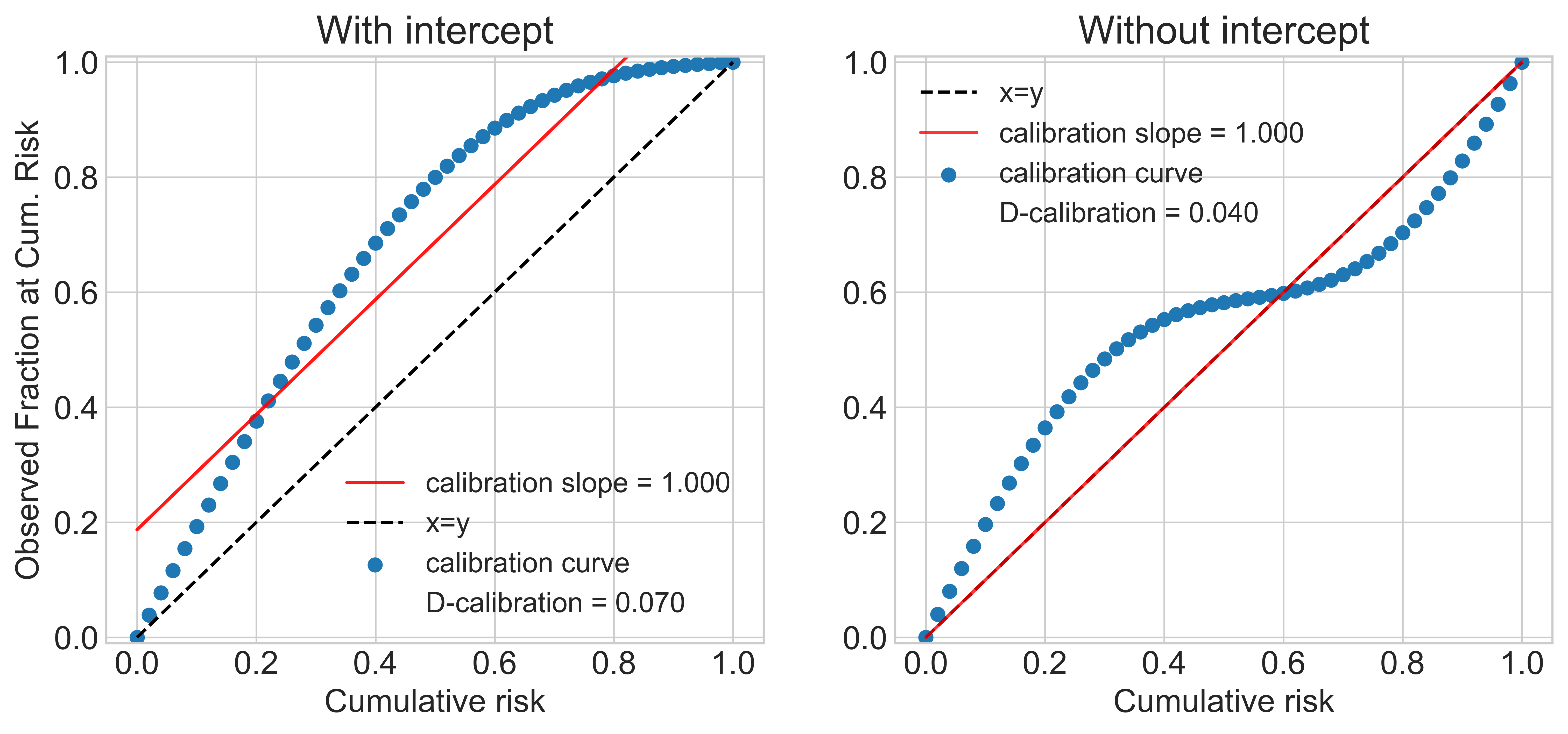
Figure 1: Sub-optimal calibration curves that result in optimal calibration slope.

Stevens and Poppe (2020) make a related observation about calibration slope: a near-zero intercept of the line of best fit, or other evidence of calibration, should always be reported alongside near-1 slope when claiming a model is calibrated. However, we demonstrate here that even slope $1$ and intercept $0$ can result from poorly calibrated models. The interested reader should see Stevens and Poppe (2020) for an assessment of recent publications in medicine that report only slope and for the history of slope-only as a “measure of spread" (Cox, 1958).

Appendix B Survival CRPS

s-crps is proposed by Avati et al. (2019):

$$\mathcal{S}_{\text{CRPS}}(\hat{F},(y,c))=\int_{0}^{y}\hat{F}(z)^{2}dz+(1-c)\int_{y}^{\infty}(1-\hat{F}(z))^{2}dz,$$

where $y$ is the event time, $c$ is an indicator for censorship and $\hat{F}$ is the cdf from the model. See Avati et al. (2019) Appendix B for a detailed derivation of s-crps objective for a log-normal model.

Appendix C CDF of Survival Time is Uniform for Censored Patient

Consider the data distribution $P(\boldsymbol{\mathbf{t}},\boldsymbol{\mathbf{c}}~{}|~{}x)$ and using the conditional $P(\boldsymbol{\mathbf{t}}~{}|~{}x)$ of this distribution to evaluate d-calibration on this data. For a point that is censored at time $c$, $P(\boldsymbol{\mathbf{t}}~{}|~{}x)$ would simply condition on the event $\boldsymbol{\mathbf{t}}>c$ for constant $c$, yielding $P(\boldsymbol{\mathbf{t}}~{}|~{}\boldsymbol{\mathbf{t}}>c,x)$. However, the true failure distribution for such a point is $P(\boldsymbol{\mathbf{t}}~{}|~{}\boldsymbol{\mathbf{t}}>c,\boldsymbol{\mathbf{c}}=c,x)$. Under censoring-at-random,

$$\boldsymbol{\mathbf{t}}\mathchoice{\mathrel{\hbox to0.0pt{$\displaystyle\perp$\hss}\mkern 2.0mu{\displaystyle\perp}}}{\mathrel{\hbox to0.0pt{$\textstyle\perp$\hss}\mkern 2.0mu{\textstyle\perp}}}{\mathrel{\hbox to0.0pt{$\scriptstyle\perp$\hss}\mkern 2.0mu{\scriptstyle\perp}}}{\mathrel{\hbox to0.0pt{$\scriptscriptstyle\perp$\hss}\mkern 2.0mu{\scriptscriptstyle\perp}}}\boldsymbol{\mathbf{c}}~{}|~{}\boldsymbol{\mathbf{x}}\implies P(\boldsymbol{\mathbf{t}}~{}|~{}\boldsymbol{\mathbf{t}}>c,x)=P(\boldsymbol{\mathbf{t}}~{}|~{}\boldsymbol{\mathbf{t}}>c,\boldsymbol{\mathbf{c}}=c,x).$$ (13)

Let $F$ be the failure cdf. Let $p_{t}$ be the density of $\boldsymbol{\mathbf{t}}~{}|~{}x$. Apply transformation $\boldsymbol{\mathbf{z}}=F(\boldsymbol{\mathbf{t}}|x)$. To compute $\boldsymbol{\mathbf{z}}$’s density, we need:

$$\frac{d}{dz}F^{-1}(z|x)=\frac{1}{p_{t}(F^{-1}(z~{}|~{}x))}=\frac{1}{p_{t}(t)}.$$

Applying change of variable to compute $\boldsymbol{\mathbf{z}}$’s density:

$$p_{t}(F^{-1}(z|x))\frac{d}{dz}F^{-1}(z|x)=p_{t}(t)\frac{1}{p_{t}(t)}=1$$

Therefore, $\boldsymbol{\mathbf{z}}$ is uniform distributed over [0,1]. So conditioning on set $(\boldsymbol{\mathbf{t}}>c,x)=(\boldsymbol{\mathbf{z}}>F(c|x),x)$ gives the result:

$$\boldsymbol{\mathbf{z}}~{}|~{}(\boldsymbol{\mathbf{t}}>c,x)\sim\text{Unif}(F(c~{}|~{}x),1).$$

The cdf value of the unobserved time for a censored datapoint is uniform above the failure cdf applied to the censoring time. Haider et al. (2020) (Appendix B) give an alternate proof in terms of expected counts.

Appendix D Extra Data Details

D.1 Data Details for Simulation Study

For the gamma simulation, we draw $\boldsymbol{\mathbf{x}}$ from a $D=32$ multivariate Normal with $\mathbf{0}$ mean and diagonal covariance with $\sigma^{2}=10.0$. We draw failure times $\boldsymbol{\mathbf{t}}$ conditionally on $\boldsymbol{\mathbf{x}}$ from a gamma distribution with mean $\boldsymbol{\mathbf{\mu}}$ log-linear in $\boldsymbol{\mathbf{x}}$. The weights of the linear function are drawn uniformly. The gamma distribution has constant variance 1e-3. This is achieved by setting $\alpha=\boldsymbol{\mathbf{\mu}}_{i}^{2}/1e\text{-}3$ and $\beta=\boldsymbol{\mathbf{\mu}}_{i}/1e\text{-}3$.

$$\boldsymbol{\mathbf{x}}_{i}\sim\mathcal{N}(0,\sigma^{2}\mathbf{I}),\quad\mathbf{w}_{d}\sim\texttt{Unif}(-0.1,0.1),\quad\boldsymbol{\mathbf{\mu}}_{i}=\exp[\mathbf{w}^{\top}\boldsymbol{\mathbf{x}}_{i}],\quad\boldsymbol{\mathbf{t}}_{i}\sim\mathtt{Gamma}(\alpha,\beta).$$

Censoring times are drawn like failure times but with a different set of weights for the linear function. This means $\boldsymbol{\mathbf{t}}\mathchoice{\mathrel{\hbox to0.0pt{$\displaystyle\perp$\hss}\mkern 2.0mu{\displaystyle\perp}}}{\mathrel{\hbox to0.0pt{$\textstyle\perp$\hss}\mkern 2.0mu{\textstyle\perp}}}{\mathrel{\hbox to0.0pt{$\scriptstyle\perp$\hss}\mkern 2.0mu{\scriptstyle\perp}}}{\mathrel{\hbox to0.0pt{$\scriptscriptstyle\perp$\hss}\mkern 2.0mu{\scriptscriptstyle\perp}}}\boldsymbol{\mathbf{c}}~{}|~{}\boldsymbol{\mathbf{x}}$.

D.2 Data Details for MNIST

As described in the main text, we follow Polsterl (2019) to simulate a survival dataset conditionally on the mnist dataset (LeCun et al., 2010). Each mnist label gets a deterministic risk score, with labels loosely grouped together by risk groups. See Table 5 for an example of the risk groups and risk scores for the mnist classes.

Datapoint image $\boldsymbol{\mathbf{x}}_{i}$ with label $\boldsymbol{\mathbf{y}}_{i}$ has time $\boldsymbol{\mathbf{t}}_{i}$ drawn from a Gamma whose mean is the risk score and whose variance is constant 1e-3. Therefore $\boldsymbol{\mathbf{t}}_{i}$ is independent of $\boldsymbol{\mathbf{x}}_{i}$ given $\boldsymbol{\mathbf{y}}_{i}$ and times for datapoints that share an mnist class are identically drawn.

$$\boldsymbol{\mu}_{i}=\text{risk}(\boldsymbol{\mathbf{y}}_{i})\quad v=1e\text{-}3\quad\alpha=\boldsymbol{\mathbf{\mu}}_{i}^{2}/v,\quad\beta=\boldsymbol{\mathbf{\mu}}_{i}/v,\quad\boldsymbol{\mathbf{t}}_{i}\sim\mathtt{Gamma}(\alpha,\beta)$$

For each split of the data (e.g. training set), we draw censoring times uniformly between the minimum failure time in that split and the $90^{th}$ percentile time, which, due to the particular failure distributions, resulted in about 50% censoring.

Table 5: Risk scores for digit classes.

Digit	0	1	2	3	4	5	6	7	8	9
Risk Group	most	least	lower	lower	lower	higher	least	most	least	most
Risk Score	11.25	2.25	5.25	5.0	4.75	8.0	2.0	11.0	1.75	10.75

D.3 Data Details for MIMIC-III

We show the 17 physiological variables we use in Table 6. The table is reproduced from Harutyunyan et al. (2017). This dataset differs from other mimic-iii length of stay datasets because one stay in the ICU of a single patient produces many datapoints: remaining time at each hour after admission. After excluding ICU transfers and patients under 18, there are $2,925,434$ and $525,912$ instances in the training and test sets. We split the training set in half for train and validation.

Table 6: The 17 selected clinical variables. The second column shows the source table(s) of a variable from mimic-iii database. The third column lists the “normal” values used in the imputation step. Table reproduced from Harutyunyan et al. (2017).

Variable table	Impute value	Modeled as
Capillary refill rate	0.0	categorical
Diastolic blood pressure	59.0	continuous
Fraction inspired oxygen	0.21	continuous
Glascow coma scale eye opening	4 spontaneously	categorical
Glascow coma scale motor response	6 obeys commands	categorical
Glascow coma scale total	15	categorical
Glascow coma scale verbal response	5 oriented	categorical
Glucose	128.0	continuous
Heart Rate	86	continuous
Height	170.0	continuous
Mean blood pressure	77.0	continuous
Oxygen saturation	98.0	continuous
Respiratory rate	19	continuous
Systolic blood pressure	118.0	continuous
Temperature	36.6	continuous
Weight	81.0	continuous
pH	7.4	continuous

D.4 Data Details for The Cancer Genome Atlas Glioma Data

We use the glioma (a type of brain cancer) data collected as part of the tcga program and studied in (Network, 2015). Tcga comprises clinical data and molecular from 11,000 patients being treated for a diverse set of cancer types. We focus on predicting time until death from the clinical data, which includes:

• tumor tissue site

• time of initial pathologic diagnosis

• radiation therapy

• Karnofsky performance score

• histological type

• demographic information

Censoring means they did not pass away. The train/validation/test sets are made of 552/276/277 datapoints respectively, of which 235/129/126 are censored, respectively.

To download this data, use the firebrowse. tool, select the Glioma (GBMLGG) cohort, and then click the blue clinical features bar on the right hand side. Select the “Clinical Pick Tier 1" file.

We standardized the features and then clamped their maximum absolute value at $5.0$. This is in part because we were working with the Weibull aft model, which is very sensitive to large variance in covariates.

Appendix E Model Descriptions

We describe the models we use in the experiments. For all models, the parameterization as a function of $\boldsymbol{\mathbf{x}}$ varies in complexity (e.g. linear or deep) depending on task.

Log-normal model

When $\log T$ is Normal with mean $\mu$ and variance $\sigma^{2}$, we say that $T$ is log-normal with location $\mu$ and scale $\sigma$. We parameterize $\mu$ and $\sigma$ as functions of $\boldsymbol{\mathbf{x}}$ (small ReLU networks with $1$ to $3$ hidden layers, depending on experiment).

Weibull Model

The Weibull Accelerated Failure Times (aft) model sets $\log T=\beta_{0}+\beta^{\top}X+\sigma W$ where $\sigma$ is a scale parameter and $W$ is Gumbel. It follows that $T\sim\text{Weibull}(\lambda,k)$ with scale $\lambda=\exp[\beta^{\top}X]$ and concentration $k=\sigma^{-1}$ (Liu, 2018). We constrain $k\in(1,2)$.

Interpolation for Discrete Models

The next two models predict for a finite set of times and therefore have a discontiuous cdf. These models have a lower-bound $\ell>0$ on d-calibration because the cdf values will not be $\text{Unif}(0,1)$ distributed. However, $\ell$ decreases to $0$ as the number of discrete times increases. For any fixed number of times, minimizing d-calibration will still improve calibration, which we observe in our experiments.

We optionally use linear interpolation to calculate the cdf. Suppose a time $t$ falls into bin $k$ which covers time interval $(t_{a},t_{b})$. If we do not use interpolation, then the cdf value $P(T\leq t)$ we calculate is the sum of the probabilities of bins whose indices are smaller than or equal to $k$. If we use linear interpolation, we replace the probability of bin $k$, $P(k)$, in the summation by:

$$\frac{t-t_{a}}{t_{b}-t_{a}}P(k)$$

Categorical Model

We parameterize a categorical distribution over discrete times by using a neural network function of $\boldsymbol{\mathbf{x}}$ with a size $B$ output. Interpreted ordinally, this can approximate continuous survival distributions as $B\to\infty$ (Lee et al., 2018; Miscouridou et al., 2018). The time for each bin is set to training data percentiles so that each next bin captures the range of times for the next $(100/B)^{th}$ percentile of training data, using only uncensored times.

Multi-Task Logistic Regression (mtlr)

mtlr differs from the Categorical Model because there is some relationship between the probability of the bins. Assume we have $K$ bins. In the linear case Yu et al. (2011), suppose our input is $x$ and parameters $\Theta=(\theta_{1},\dots,\theta_{K-1})$. The probability for bin $k<K$ is:

$$\frac{\exp(\sum_{j=k}^{K-1}\theta_{j}^{T}x)}{1+\sum_{i=1}^{K-1}\exp(\sum_{j=i}^{K-1}\theta_{j}^{T}x)},$$

and the probability for bin $K$ is :

$$\frac{1}{1+\sum_{i=1}^{K-1}\exp(\sum_{j=i}^{K-1}\theta_{j}^{T}x)}.$$

Appendix F Experimental Details

F.1 Gamma Simulation

We use a $4$-layer neural network of hidden-layer sizes $128,64,64$ units, with ReLU activations to parameterize the categorical and log-normal distributions. For categorical we use another linear transformation to map to 50 output dimensions. For the log-normal model, two copies of the above neural network are used, one to output the location and the other to output the log of the log-normal scale parameter. For mtlr, we use a linear transformation from covariates to 50 dimensions and use a softmax layer to output the probability for the 50 bins. We use $0$ dropout, $0$ weight decay, learning rate 1e-3 and batch size 1000 for 100 epochs in this experiment.

F.2 Survial MNIST

The model does not see the mnist class and learns a distribution over times given pixels $\boldsymbol{\mathbf{x}}_{i}$. We use a convolutional neural network. We use several layers of 2D convolutions with a kernel of size $2$ and stride of size $1$. The sequence of channel numbers is $32,64,128,256$ with the last layer containing scalars. After each convolution, we use ReLU, then dropout, then size $2$ max pooling.

For categorical and log-normal models, this CNN output is mapped through a three-hidden-layer ReLU neural network with hidden sizes $512,1024,1024$. Between the fully connected layers, we use ReLU then dropout. Again, with the log-normal, separate networks are used to output the location and log-scale. For mtlr, the CNN output is linearly mapped to the 50 bins. For categorical, we use $0.2$ dropout for uncensored and $0.1$ for censored. In mtlr, we use dropout $0.2$. In lognormal, we use dropout $0.1$. We use weight decay 1e-4, learning rate 1e-3, and batch size 5000 for 200 epochs.

F.3 MIMIC-III

The input is high-dimensional (about $1400$) because it is a concatenated time series and because missingness masks are used. We use a 4-layer neural network of hidden-layer sizes $2048,1024,1024$ units with ReLU activations. For the categorical model, we use $B=20$ categorical output bins. For the log-normal model, we use one three-hidden neural network of hidden-layer sizes $128,64,64$ units and an independent copy to output the location and log-scale parameters. We use dropout $0.15$, learning rate 1e-3 and weight decay 1e-4 for 200 epochs at batch size 5000.

F.4 The Cancer Genome Atlas, Glioma

The Weibull model has parameters scale and concentration. The scale is set to $\exp[\beta^{\top}\boldsymbol{\mathbf{x}}]$ for regression parameters $\beta$, plus a constant $1.0$ for numerical stability. We optimize the concentration parameter in $(1,2)$. The log-normal model is as described in the simulated gamma experiment, except that it has two instead of three hidden layers, due to small data sample size. The categorical and mtlr models are also as described in the simulated gamma experiment, except that they have 20 instead of 50 bins, and are linear, again due to small data sample size.

We standardize this data and then clamp all covariates at absolute value $5.0$. For all models, we train for 10,000 epochs at learning rate 1e-2 with full data batch size 1201. We use 10 d-calibration bins for this experiment as studied in Haider et al. (2020), rather than the 20 bins used in all other experiments.

Appendix G Exploring Choice of $\gamma$ soft-indicator parameter

There is a trade-off in setting the soft membership parameter $\gamma$. Larger values approximate the indicator function better, but can have worse gradients because the values lie in the flat region of the sigmoid. See Figure 2 for an example of how gamma changes the soft indicator for a given set $I=[0.45,0.55]$.

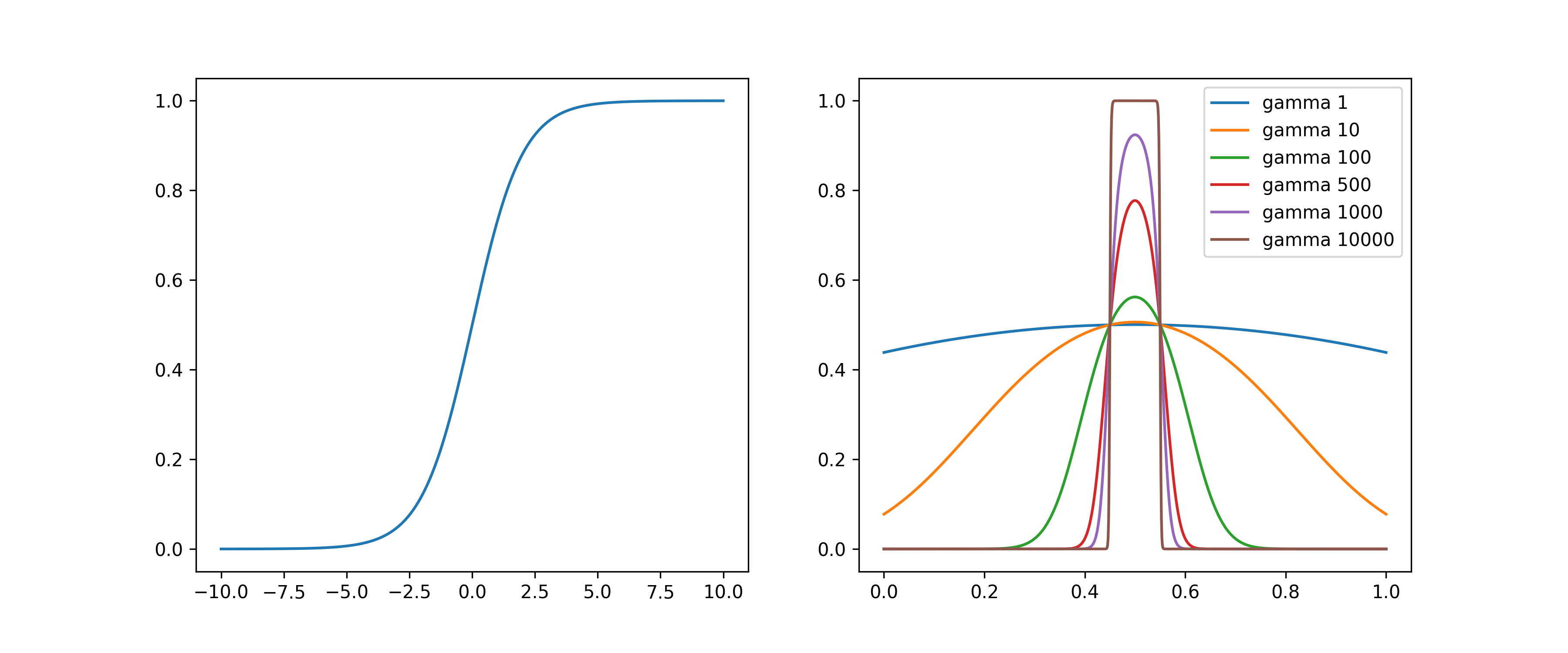
Figure 2: Left: the sigmoid function. Right: choice of hyper-parameter gamma in soft indicator function for set $I=[0.45,0.55]$.

We choose $\gamma=10000$ in all of the experiments and find that it allows us to minimize exact d-cal (d-cal). We explore other choices in Table 7. We see the expected improvement in approximation as $\gamma$ increases. Then, as $\gamma$ gets too large, exact d-cal stops improving as a function of $\lambda$.

Table 7: Exact D-Cal, Soft-Dcal, and NLL at end of training, evaluated on training data for models trained with $\lambda=10$ and batch size $1,000$. Approximation improves as $\gamma$ increases. Gradients vanish when $\gamma$ gets too large. All experiments are better in calibration than the $\lambda=0$ MLE model, which has exact D-cal $0.09$.

$\gamma$	$10$	$10^{2}$	$10^{3}$	$10^{4}$	$10^{5}$	$10^{6}$	$10^{7}$	$5\times 10^{7}$
Exact D-Cal	$0.2337$	$0.0095$	$0.0079$	$0.0039$	$0.0025$	$0.0014$	$0.0015$	$0.0048$
Soft D-Cal	$0.4599$	$0.0604$	$0.0074$	$0.0039$	$0.0025$	$0.0014$	$0.0015$	$0.0048$
NLL	$2.1180$	$1.1362$	$1.0793$	$1.2508$	$1.6993$	$2.3873$	$2.6940$	$3.4377$

Appendix H Exploring Slack due to Jensen’s Inequality

We trained the Categorical model on the gamma simulation data with $\gamma=10,000$ and batch size $10,000$ for all $\lambda$. The trained models are evaluated on the training set (size $100,000$) with two different test batch sizes, $500$ and $1000$. Table 8 demonstrates that the upper-bounds for both batch sizes preserve model ordering with respect to exact d-calibration. The bound for batch size $10,000$ is quite close to the exact d-calibration.

Table 8: Slack in the upper-bound preserves modeling ordering with respect to exact d-calibration

$\lambda$	Batch Size	Exact D-Cal	Upper-bound
$0$	$500$	$0.05883$	$0.0605$
	$10000$	”	$0.0589$
$1$	$500$	$0.02204$	$0.0238$
	$10000$	”	$0.0221$
$5$	$500$	$0.00963$	$0.0114$
	$10000$	”	$0.0097$
$10$	$500$	$0.00482$	$0.0066$
	$10000$	”	$0.0048$
$50$	$500$	$0.00040$	$0.0021$
	$10000$	”	$0.0004$
$100$	$500$	$0.00022$	$0.0021$
	$10000$	”	$0.0003$
$500$	$500$	$0.00015$	$0.0020$
	$10000$	”	$0.0002$
$1000$	$500$	$0.00006$	$0.0019$
	$10000$	”	$0.0001$

Appendix I Modification of soft indicator for the first and the last interval

In our soft indicator,

$$\zeta_{\gamma}(u;I)=\text{Sigmoid}(\gamma(u-a)(b-u))=\left(1+\exp(-\gamma(u-a)(b-u))\right)^{-1}$$

is a differentiable approximation for $\mathbbm{1}\left[u\in[a,b]\right]$. When $b$ is the upper boundary of all the $u$ values, for example, 1 for cdf values, the $b$ in the soft indicator can be replaced by any value that is greater than $b$. We use 2 to replace 1 for the upper boundary when $b=1$ in our experiments. Similarly we use $a=-1$ to replace $a=0$ for the lower boundary when $a=0$.

Consider the term in our upper-bound (eq. 6) for the last interval $I=[a,b]$, where $b=1$, $\left(\frac{1}{M}\sum_{i}\zeta_{\gamma}(u_{i};I)-|I|\right)^{2}$. The gradient of this term with respect to one cdf value $u_{i}$ is:

$$\frac{d}{du_{i}}\left(\frac{1}{M}\sum_{i}\zeta_{\gamma}(u_{i};I)-|I|\right)^{2}$$

$$= \frac{d}{du_{i}}\left(\frac{1}{M}\sum_{i}\text{Sigmoid}(\gamma(u_{i}-a)(b-u_{i}))-|I|\right)^{2}$$

$$\Bigg{[}\text{ let }A:=2/M*\left(\frac{1}{M}\sum_{i}\text{Sigmoid}(\gamma(u_{i}-a)(b-u_{i}))-|I|\right)\Bigg{]}$$

$$= A\frac{d}{du_{i}}\text{Sigmoid}(\gamma(u_{i}-a)(b-u_{i}))$$

$$= A*-\frac{\exp(-\gamma(u_{i}-a)(b-u_{i}))}{(1+\exp(-\gamma(u_{i}-a)(b-u_{i})))^{2}}\frac{d}{du_{i}}\left(-\gamma(u_{i}-a)(b-u_{i})\right)$$

$$= A*\frac{\exp(-\gamma(u_{i}-a)(b-u_{i}))}{(1+\exp(-\gamma(u_{i}-a)(b-u_{i})))^{2}}*\gamma*(a+b-2u_{i})$$

If

$$\frac{1}{M}\sum_{i}\zeta_{\gamma}(u_{i};I)-|I|>0,$$

then the fraction of points in the interval is larger than the size of the interval. We want to move the points out of the interval. In the last interval, in order to move points out of the interval, we can only make the values smaller, which means we want the gradient with respect to $u$ to be positive. (recall that we are moving in the direction of the negative gradient to minimize the objective). However, for points that are greater than $(a+b)/2$, the above gradient will be negative because term $(a+b-2u_{i})$ is negative. This is not ideal. Changing the value $b$ from 1 to 2 can resolve the issue. Since cdf values are all smaller than 1, $(a+b)/2$ will always be greater than $u$ if we use $b=2$ for the last interval. The above optimization issue only applies on the first and last interval because for intervals in the middle, we can move the points either to left or right to lower the fraction of points in the interval.

Appendix J Full Results: More Models and Choices of Lambda

Table 9: Gamma simulation, uncensored (full results)

	$\lambda$	0	1	5	10	50	100	500	1000
Log-Norm	nll	0.381	0.423	0.507	0.580	0.763	0.809	0.870	0.882
nll	d-cal	0.271	0.060	0.021	0.011	0.001	4e-4	1e-4	7e-5
	conc	0.982	0.955	0.931	0.908	0.841	0.835	0.809	0.802
Log-Norm	nll	0.455	0.614	0.730	0.781	0.837	0.848	0.869	0.965
s-crps	d-cal	0.055	0.014	0.004	0.002	2e-4	1e-4	1e-4	1e-4
	conc	0.979	0.975	0.968	0.959	0.940	0.931	0.864	0.811
Cat-ni	nll	0.998	1.042	1.129	1.197	1.788	2.098	3.148	3.688
	d-cal	0.074	0.023	0.008	0.005	4e-4	4e-4	2e-4	1e-4
	conc	0.986	0.986	0.985	0.985	0.973	0.960	0.877	0.748
Cat-i	nll	0.997	1.001	1.029	1.083	1.763	2.083	3.167	3.788
	d-cal	0.002	0.002	0.001	0.002	5e-4	5e-4	1e-4	1e-4
	conc	0.986	0.986	0.986	0.985	0.972	0.960	0.874	0.699
mtlr-NI	nll	1.287	1.409	1.589	1.612	2.356	2.590	3.267	3.509
	d-cal	0.027	0.027	0.015	0.008	5e-4	2e-4	2e-4	2e-4
	conc	0.986	0.986	0.983	0.981	0.952	0.940	0.909	0.899
mtlr-I	nll	1.392	1.419	1.616	1.823	2.165	2.612	2.982	3.184
	d-cal	0.048	0.034	0.017	0.009	7e-4	2e-4	1e-4	1e-4
	conc	0.986	0.986	0.982	0.980	0.958	0.934	0.918	0.917

Table 10: Gamma simulation, censored (full results). For categorical model with interpolation, the d-cal is already very low at $\lambda=0$ so it is hard to optimize this one further.

	$\lambda$	0	1	5	10	50	100	500	1000
Log-Norm	nll	-0.059	-0.049	-0.022	0.004	0.099	0.138	0.191	0.215
nll	d-cal	0.029	0.020	0.008	0.005	7e-4	2e-4	6e-5	7e-5
	conc	0.981	0.969	0.950	0.942	0.927	0.916	0.914	0.897
Log-Norm	nll	0.038	0.084	0.119	0.143	0.185	0.201	0.343	0.436
s-crps	d-cal	0.017	0.007	0.003	0.001	1e-4	1e-4	5e-5	8e-5
	conc	0.982	0.978	0.971	0.963	0.952	0.950	0.850	0.855
Cat-ni	nll	0.797	0.799	0.805	0.822	1.023	1.149	1.665	1.920
	d-cal	0.009	0.006	0.003	0.002	3e-4	2e-4	6e-5	6e-5
	conc	0.987	0.987	0.987	0.987	0.982	0.976	0.922	0.861
Cat-i	nll	0.783	0.782	0.788	0.795	0.948	1.124	1.686	1.994
	d-cal	7e-5	1e-4	6e-5	8e-5	2e-4	2e-4	4e-5	6e-5
	conc	0.987	0.987	0.987	0.987	0.983	0.976	0.933	0.847
mtlr-NI	nll	0.873	0.875	0.875	0.977	1.271	1.412	1.747	1.900
	d-cal	0.004	0.004	0.003	0.004	4e-4	2e-4	2e-4	2e-4
	conc	0.987	0.987	0.987	0.985	0.973	0.965	0.951	0.943
mtlr-I	nll	0.829	0.830	0.866	0.981	1.266	1.414	1.762	1.912
	d-cal	0.004	0.004	0.004	0.004	5e-4	1e-4	6e-5	7e-5
	conc	0.988	0.988	0.987	0.985	0.971	0.963	0.947	0.939

Table 11: Survival-mnist, uncensored (full results)

	$\lambda$	0	1	5	10	50	100	500	1000
Log-Norm	nll	4.344	4.407	4.530	4.508	4.549	4.571	5.265	5.417
nll	d-cal	0.328	0.104	0.018	0.020	0.011	0.010	0.005	0.005
	conc	0.886	0.867	0.754	0.759	0.725	0.713	0.541	0.509
Log-Norm	nll	4.983	4.940	4.853	4.759	4.714	4.673	4.852	5.118
s-crps	d-cal	0.212	0.132	0.081	0.059	0.020	0.007	0.003	0.003
	conc	0.889	0.878	0.866	0.861	0.873	0.873	0.820	0.798
Cat-ni	nll	1.726	1.730	1.737	1.755	1.824	1.860	2.076	3.073
	d-cal	0.019	0.013	0.008	0.005	9e-4	9e-4	6e-4	3e-4
	conc	0.945	0.945	0.945	0.937	0.921	0.916	0.854	0.690
Cat-i	nll	1.726	1.731	1.735	1.741	1.782	1.809	1.953	2.157
	d-cal	0.007	0.005	0.003	0.002	6e-4	3e-4	4e-4	3e-4
	conc	0.945	0.945	0.945	0.945	0.940	0.937	0.897	0.830
mtlr-ni	nll	1.747	1.745	1.749	1.772	1.832	1.850	2.075	2.419
	d-cal	0.018	0.014	0.008	0.004	0.001	0.001	8e-4	0.002
	conc	0.944	0.945	0.945	0.944	0.934	0.934	0.870	0.808
mtlr-I	nll	1.746	1.746	1.752	1.756	1.779	1.802	1.975	2.560
	d-cal	0.005	0.004	0.003	0.002	5e-4	4e-4	8e-4	0.001
	conc	0.944	0.944	0.945	0.944	0.941	0.936	0.886	0.806

Table 12: Survival-mnist, censored (full results)

	$\lambda$	0	1	5	10	50	100	500	1000
Log-Norm	nll	4.337	4.377	4.433	4.483	4.602	4.682	4.914	5.151
nll	d-cal	0.392	0.074	0.033	0.020	0.008	0.005	0.005	0.007
	conc	0.902	0.873	0.829	0.794	0.728	0.696	0.628	0.573
Log-Norm	nll	4.950	4.929	4.873	4.859	4.672	4.749	4.786	4.877
s-crps	d-cal	0.215	0.122	0.071	0.051	0.018	0.010	0.002	9e-4
	conc	0.891	0.881	0.871	0.874	0.866	0.868	0.839	0.815
Cat-ni	nll	1.733	1.734	1.738	1.765	1.827	1.861	2.074	3.030
	d-cal	0.018	0.014	0.008	0.004	8e-4	5e-4	5e-4	4e-4
	conc	0.945	0.945	0.944	0.927	0.920	0.919	0.862	0.713
Cat-i	nll	1.731	1.731	1.741	1.750	1.779	1.805	1.955	2.113
	d-cal	0.007	0.006	0.003	0.002	3e-4	4e-4	4e-4	3e-4
	conc	0.945	0.944	0.945	0.945	0.942	0.938	0.901	0.843
mtlr-NI	nll	1.126	1.118	1.125	1.136	1.174	1.193	1.350	1.482
	d-cal	0.021	0.017	0.012	0.009	0.006	0.006	0.006	0.007
	conc	0.958	0.960	0.961	0.960	0.949	0.943	0.897	0.880
mtlr-I	nll	1.126	1.118	1.125	1.136	1.174	1.193	1.350	1.482
	d-cal	0.021	0.017	0.012	0.009	0.006	0.006	0.006	0.007
	conc	0.958	0.960	0.961	0.960	0.949	0.943	0.897	0.880

Table 13: mimic-iii length of stay (full results)

	$\lambda$	0	1	5	10	50	100	500	1000
Log-Norm	d-cal	0.860	0.639	0.210	0.155	0.066	0.046	0.009	0.005
s-crps	conc	0.625	0.639	0.577	0.575	0.558	0.555	0.528	0.506
Cat-ni	nll	3.142	3.177	3.101	3.167	3.086	3.088	3.448	3.665
	d-cal	0.002	0.002	0.002	0.001	3e-4	2e-4	1e-4	1e-4
	conc	0.702	0.700	0.701	0.699	0.695	0.690	0.642	0.627
Cat-i	nll	3.142	3.075	3.157	3.073	3.002	3.073	3.364	3.708
	d-cal	4-e4	3e-4	3e-4	3e-4	4e-4	1e-4	5e-5	4e-5
	conc	0.702	0.702	0.701	0.702	0.698	0.695	0.638	0.627

Table 14: The Cancer Genome Atlas, glioma (full results)

	$\lambda$	0	1	5	10	50	100	500	1000
Weibull	nll	4.436	4.390	4.313	4.292	4.441	4.498	4.475	4.528
	d-cal	0.035	0.028	0.014	0.009	0.003	0.003	0.004	0.007
	conc	0.788	0.785	0.781	0.777	0.731	0.702	0.608	0.575
Log-Norm	nll	14.187	6.585	4.841	4.639	4.181	4.181	4.403	4.510
nll	d-cal	0.059	0.024	0.012	0.010	0.003	0.003	0.002	0.004
	conc	0.657	0.632	0.673	0.703	0.778	0.805	0.474	0.387
Log-Norm	nll	5.784	5.801	5.731	5.698	5.047	4.892	4.750	4.712
s-crps	d-cal	0.258	0.2585	0.257	0.252	0.100	0.0702	0.044	0.025
	conc	0.798	0.798	0.798	0.810	0.568	0.507	0.420	0.363
Cat-ni	nll	1.718	1.742	1.746	1.758	1.800	1.799	1.810	1.826
	d-cal	0.008	0.003	0.002	0.002	0.003	0.003	0.003	0.002
	conc	0.781	0.771	0.775	0.775	0.765	0.765	0.758	0.748
Cat-i	nll	1.711	1.718	1.733	1.726	1.743	1.787	1.781	1.789
	d-cal	0.003	0.001	8e-4	0.001	0.002	0.002	0.002	0.002
	conc	0.778	0.779	0.780	0.798	0.804	0.803	0.806	0.802
mtlr-NI	nll	1.624	1.620	1.636	1.636	1.666	1.658	1.748	1.758
	d-cal	0.009	0.007	0.007	0.005	0.003	0.003	0.002	0.002
	conc	0.828	0.829	0.822	0.824	0.814	0.818	0.788	0.763
mtlr-I	nll	1.616	1.626	1.612	1.612	1.632	1.640	1.636	1.753
	d-cal	0.003	0.003	0.002	0.001	0.001	0.001	9e-4	0.001
	conc	0.827	0.825	0.831	0.829	0.824	0.823	0.825	0.783

References

- Alaa and van der Schaar (2017) A. M. Alaa and M. van der Schaar. Deep multi-task gaussian processes for survival analysis with competing risks. In Proceedings of the 31st International Conference on Neural Information Processing Systems, pages 2326–2334. Curran Associates Inc., 2017.
- Andersen et al. (2012) P. K. Andersen, O. Borgan, R. D. Gill, and N. Keiding. Statistical models based on counting processes. Springer Science & Business Media, 2012.
- Avati et al. (2019) A. Avati, T. Duan, S. Zhou, K. Jung, N. H. Shah, and A. Y. Ng. Countdown regression: Sharp and calibrated survival predictions. In A. Globerson and R. Silva, editors, Proceedings of the Thirty-Fifth Conference on Uncertainty in Artificial Intelligence, UAI 2019, Tel Aviv, Israel, July 22-25, 2019, page 28. AUAI Press, 2019. URL http://auai.org/uai2019/proceedings/papers/28.pdf.
- Barber et al. (2019) R. F. Barber, E. J. Candes, A. Ramdas, and R. J. Tibshirani. The limits of distribution-free conditional predictive inference. arXiv preprint arXiv:1903.04684, 2019.
- Besseling et al. (2017) J. Besseling, J. B. Reitsma, D. Gaudet, D. Brisson, J. J. Kastelein, G. K. Hovingh, and B. A. Hutten. Selection of individuals for genetic testing for familial hypercholesterolaemia: development and external validation of a prediction model for the presence of a mutation causing familial hypercholesterolaemia. European heart journal, 38(8):565–573, 2017.
- Brier and Allen (1951) G. W. Brier and R. A. Allen. Verification of weather forecasts. In Compendium of meteorology, pages 841–848. Springer, 1951.
- Cox (1958) D. R. Cox. Two further applications of a model for binary regression. Biometrika, 45(3/4):562–565, 1958.
- D’agostino and Nam (2003) R. D’agostino and B.-H. Nam. Evaluation of the performance of survival analysis models: discrimination and calibration measures. Handbook of statistics, 23:1–25, 2003.
- Davidson-Pilon et al. (2017) C. Davidson-Pilon, J. Kalderstam, N. Jacobson, P. Zivich, B. Kuhn, M. Williamson, A. Moncada-Torres, K. Stark, S. Anton, J. Noorbakhsh, et al. Camdavidsonpilon/lifelines: v0.24.0. Context, 604(40F), 2017.
- Demler et al. (2015) O. V. Demler, N. P. Paynter, and N. R. Cook. Tests of calibration and goodness-of-fit in the survival setting. Statistics in medicine, 34(10):1659–1680, 2015.
- George et al. (2014) B. George, S. Seals, and I. Aban. Survival analysis and regression models. Journal of nuclear cardiology, 21(4):686–694, 2014.
- Gerds and Schumacher (2006) T. A. Gerds and M. Schumacher. Consistent estimation of the expected brier score in general survival models with right-censored event times. Biometrical Journal, 48(6):1029–1040, 2006.
- Giunchiglia et al. (2018) E. Giunchiglia, A. Nemchenko, and M. van der Schaar. Rnn-surv: A deep recurrent model for survival analysis. In International Conference on Artificial Neural Networks, pages 23–32. Springer, 2018.
- Graf et al. (1999) E. Graf, C. Schmoor, W. Sauerbrei, and M. Schumacher. Assessment and comparison of prognostic classification schemes for survival data. Statistics in medicine, 18(17-18):2529–2545, 1999.
- Gronnesby and Borgan (1996) J. K. Gronnesby and O. Borgan. A method for checking regression models in survival analysis based on the risk score. Lifetime data analysis, 2(4):315–328, 1996.
- Guo et al. (2017) C. Guo, G. Pleiss, Y. Sun, and K. Q. Weinberger. On calibration of modern neural networks. In Proceedings of the 34th International Conference on Machine Learning-Volume 70, pages 1321–1330. JMLR. org, 2017.
- Haider et al. (2020) H. Haider, B. Hoehn, S. Davis, and R. Greiner. Effective ways to build and evaluate individual survival distributions. Journal of Machine Learning Research, 21(85):1–63, 2020.
- Harrell Jr et al. (1996) F. E. Harrell Jr, K. L. Lee, and D. B. Mark. Multivariable prognostic models: issues in developing models, evaluating assumptions and adequacy, and measuring and reducing errors. Statistics in medicine, 15(4):361–387, 1996.
- Harutyunyan et al. (2017) H. Harutyunyan, H. Khachatrian, D. C. Kale, G. V. Steeg, and A. Galstyan. Multitask learning and benchmarking with clinical time series data. arXiv preprint arXiv:1703.07771, 2017.
- Horvitz and Thompson (1952) D. G. Horvitz and D. J. Thompson. A generalization of sampling without replacement from a finite universe. Journal of the American statistical Association, 47(260):663–685, 1952.
- Johnson et al. (2016) A. E. Johnson, T. J. Pollard, L. Shen, H. L. Li-wei, M. Feng, M. Ghassemi, B. Moody, P. Szolovits, L. A. Celi, and R. G. Mark. Mimic-iii, a freely accessible critical care database. Scientific data, 3:160035, 2016.
- Kalbfleisch and Prentice (2002) J. D. Kalbfleisch and R. L. Prentice. The Statistical Analysis of Failure Time Data. Wiley Series in Probability and Statistics. John Wiley & Sons, Inc., 2 edition, 2002.
- Kaplan and Meier (1958) E. L. Kaplan and P. Meier. Nonparametric estimation from incomplete observations. Journal of the American statistical association, 53(282):457–481, 1958.
- Katzman et al. (2018) J. L. Katzman, U. Shaham, A. Cloninger, J. Bates, T. Jiang, and Y. Kluger. Deepsurv: personalized treatment recommender system using a cox proportional hazards deep neural network. BMC medical research methodology, 18(1):24, 2018.
- Kumar et al. (2018) A. Kumar, S. Sarawagi, and U. Jain. Trainable calibration measures for neural networks from kernel mean embeddings. In International Conference on Machine Learning, pages 2805–2814, 2018.
- Kvamme and Borgan (2019) H. Kvamme and O. Borgan. The brier score under administrative censoring: Problems and solutions. arXiv preprint arXiv:1912.08581, 2019.
- Lawless (2011) J. F. Lawless. Statistical Models and Methods for Lifetime Data. Wiley Series in Probability and Statistics. John Wiley & Sons, Inc., 2 edition, 2011.
- LeCun et al. (2010) Y. LeCun, C. Cortes, and C. Burges. Mnist handwritten digit database. ATT Labs [Online]. Available: http://yann.lecun.com/exdb/mnist, 2, 2010.
- Lee et al. (2018) C. Lee, W. R. Zame, J. Yoon, and M. van der Schaar. Deephit: A deep learning approach to survival analysis with competing risks. In Thirty-Second AAAI Conference on Artificial Intelligence, 2018.
- Lemeshow and Hosmer Jr (1982) S. Lemeshow and D. W. Hosmer Jr. A review of goodness of fit statistics for use in the development of logistic regression models. American journal of epidemiology, 115(1):92–106, 1982.
- Liu (2018) E. Liu. Using weibull accelerated failure time regression model to predict survival time and life expectancy. BioRxiv, page 362186, 2018.
- Matheson and Winkler (1976) J. E. Matheson and R. L. Winkler. Scoring rules for continuous probability distributions. Management science, 22(10):1087–1096, 1976.
- Miscouridou et al. (2018) X. Miscouridou, A. Perotte, N. Elhadad, and R. Ranganath. Deep survival analysis: Nonparametrics and missingness. In Machine Learning for Healthcare Conference, pages 244–256, 2018.
- Network (2015) C. G. A. R. Network. Comprehensive, integrative genomic analysis of diffuse lower-grade gliomas. New England Journal of Medicine, 372(26):2481–2498, 2015.
- Niculescu-Mizil and Caruana (2005) A. Niculescu-Mizil and R. Caruana. Predicting good probabilities with supervised learning. In Proceedings of the 22nd international conference on Machine learning, pages 625–632, 2005.
- Pepe and Janes (2013) M. Pepe and H. Janes. Methods for evaluating prediction performance of biomarkers and tests. In Risk assessment and evaluation of predictions, pages 107–142. Springer, 2013.
- Platt (1999) J. C. Platt. Probabilistic outputs for support vector machines and comparisons to regularized likelihood methods. In ADVANCES IN LARGE MARGIN CLASSIFIERS, pages 61–74. MIT Press, 1999.
- Polsterl (2019) S. Polsterl. Sebastian polsterl, Jul 2019. URL https://k-d-w.org/blog/2019/07/survival-analysis-for-deep-learning/.
- Ranganath et al. (2016) R. Ranganath, A. Perotte, N. Elhadad, and D. Blei. Deep survival analysis. arXiv preprint arXiv:1608.02158, 2016.
- Ren et al. (2019) K. Ren, J. Qin, L. Zheng, Z. Yang, W. Zhang, L. Qiu, and Y. Yu. Deep recurrent survival analysis. In Proceedings of the AAAI Conference on Artificial Intelligence, volume 33, pages 4798–4805, 2019.
- Royston and Altman (2013) P. Royston and D. G. Altman. External validation of a cox prognostic model: principles and methods. BMC medical research methodology, 13(1):33, 2013.
- Song et al. (2019) H. Song, T. Diethe, M. Kull, and P. Flach. Distribution calibration for regression. In International Conference on Machine Learning, pages 5897–5906, 2019.
- Stevens and Poppe (2020) R. J. Stevens and K. K. Poppe. Validation of clinical prediction models: what does the “calibration slope” really measure? Journal of clinical epidemiology, 118:93–99, 2020.
- Sullivan et al. (2004) L. M. Sullivan, J. M. Massaro, and R. B. D’Agostino Sr. Presentation of multivariate data for clinical use: The framingham study risk score functions. Statistics in medicine, 23(10):1631–1660, 2004.
- Vasan et al. (2008) R. S. Vasan, M. J. Pencina, P. A. Wolf, M. Cobain, J. M. Massaro, and W. B. Kannel. General cardiovascular risk profile for use in primary care. 2008.
- Vovk et al. (2005) V. Vovk, A. Gammerman, and G. Shafer. Algorithmic learning in a random world. Springer Science & Business Media, 2005.
- Wilson et al. (1998) P. W. Wilson, R. B. D’Agostino, D. Levy, A. M. Belanger, H. Silbershatz, and W. B. Kannel. Prediction of coronary heart disease using risk factor categories. Circulation, 97(18):1837–1847, 1998.
- Yadlowsky et al. (2019) S. Yadlowsky, S. Basu, and L. Tian. A calibration metric for risk scores with survival data. In Machine Learning for Healthcare Conference, pages 424–450, 2019.
- Yu et al. (2011) C.-N. Yu, R. Greiner, H.-C. Lin, and V. Baracos. Learning patient-specific cancer survival distributions as a sequence of dependent regressors. In Advances in Neural Information Processing Systems, pages 1845–1853, 2011.
- Zadrozny and Elkan (2002) B. Zadrozny and C. Elkan. Transforming classifier scores into accurate multiclass probability estimates. In Proceedings of the eighth ACM SIGKDD international conference on Knowledge discovery and data mining, pages 694–699, 2002.