Efficient integration of gradient flow in lattice gauge theory and
properties of low-storage commutator-free Lie group methods

Abstract

The smoothing procedure known as the gradient flow that suppresses ultraviolet fluctuations of gauge fields plays an important role in lattice gauge theory calculations. In particular, this procedure is often used for high-precision scale setting and renormalization of operators. The gradient flow equation is defined on the $\mbox{{SU}}(3)$ manifold and therefore requires geometric, or structure-preserving, integration methods to obtain its numerical solutions. We examine the properties and origins of the three-stage third-order explicit Runge-Kutta Lie group integrator commonly used in the lattice gauge theory community, demonstrate its relation to $2N$-storage classical Runge-Kutta methods and explore how its coefficients can be tuned for optimal performance in integrating the gradient flow. We also compare the performance of the tuned method with two third-order variable step size methods. Next, based on the recently established connection between low-storage Lie group integrators and classical $2N$-storage Runge-Kutta methods, we study two fourth-order low-storage methods that provide a computationally efficient alternative to the commonly used third-order method while retaining the convenient iterative property of the latter. Finally, we demonstrate that almost no coding effort is needed to implement the low-storage Lie group methods into existing gradient flow codes.

1ALG@line

1 Introduction

In lattice gauge theory [1], a numerical approach to quantum gauge theories, the path integrals are evaluated by sampling the space of possible field configurations with a Markov Chain Monte Carlo process and averaging over the Monte Carlo time series. The fields are defined on a four-dimensional Euclidean space-time grid and for the physically relevant case of Quantum Chromodynamics (QCD) take values in the $\mbox{{SU}}(3)$ group.

A smoothing procedure, referred to as gradient flow, introduced by Lüscher in Ref. [2], allows one to evolve a given gauge field configuration towards the classical solution. The gradient flow possesses renormalizing properties and is often used for renormalization of operators and determining the lattice spacing in physical units. Certain lattice calculations require determination of the lattice scale to sub-percent precision. Numerically, gradient flow amounts to integrating a first-order differential equation on the $\mbox{{SU}}(3)$ manifold. While a variety of structure-preserving integration methods can be used for this task [3], the three-stage third-order explicit Runge-Kutta integrator introduced in Ref. [2] became the most commonly used method in lattice gauge theory applications.

In this paper we explore the recently observed relations between classical low-storage explicit Runge-Kutta methods and the commutator-free Lie group methods [4]. We show how a three-stage third-order integrator can be optimized specifically for integrating the gradient flow and how higher-order methods with similar low-storage properties can be constructed.

The paper is organized as follows. In Sec. 2 we introduce the formalism of lattice gauge theory and gradient flow. In Sec. 3 we review the properties of standard explicit Runge-Kutta integration methods and so-called low-storage Runge-Kutta methods. In Sec. 4 we discuss structure-preserving integrators, often called geometric integrators or Lie group integrators. In Sec. 5 we present the numerical results on integrating the gradient flow on three lattice ensembles with several third- and fourth-order Lie group methods. We present our conclusions and recommendations for tuning the methods and improving the computational efficiency of integrating the gradient flow in Sec. 6.

2 Lattice gauge theory and the gradient flow

In lattice gauge theory the primary degrees of freedom are $\mbox{{SU}}(3)$ matrices $U_{x,\,\mu}$ that reside on the links of a hypercubic lattice with dimensions $N_{\sigma}^{3}\times N_{\tau}$. The lattice spacing is $a$, $x$ is an integer-valued four-vector, and $\mu=1,\dots,4$. Gauge-invariant observables are represented as traces of products of the gauge link variables along paths on the lattice that are closed loops. The main observables we discuss here are the plaquette (4-link loop):

$$P_{x,\,\mu,\nu}=U_{x,\,\mu}U_{x+\mu,\,\nu}U^{\dagger}_{x+\nu,\,\mu}U^{\dagger}_{x,\,\nu}$$ (1)

rectangle (6-link loop):

$$R_{x,\,\mu,\nu}=U_{x,\,\mu}U_{x+\mu,\,\mu}U_{x+2\mu,\,\nu}U^{\dagger}_{x+\mu+\nu,\,\mu}U^{\dagger}_{x+\nu,\,\mu}U^{\dagger}_{x,\,\nu}$$ (2)

and the so called clover expression constructed as a linear combination of several plaquettes forming the shape of a clover leaf:

$$C_{x,\,\mu,\nu}=\frac{i}{8}\left(Q_{x,\,\nu,\,\mu}-Q_{x,\,\mu,\nu}\right)$$ (3)

where $Q_{x,\,\mu,\nu}=P_{x,\,\mu,\nu}+P_{x,\nu,-\mu}+P_{x,-\mu,-\nu}+P_{x,-\nu,\,\mu}$.

The simplest gauge action is the Wilson action [1] that includes only the plaquette term (for convenience we drop the factor $1/g_{0}^{2}$ in the definition):

$$S_{Wilson}=2\sum_{x}\sum_{\mu<\nu}{\rm Re}{\rm Tr}(1-P_{x,\,\mu,\nu}).$$ (4)

To suppress lattice discretization effects one can construct improved actions such as, for instance, the tree-level Symanzik-improved gauge action that includes the plaquette and rectangle terms [5]:

$$S_{S\!ymanzik}=\frac{5}{3}S_{Wilson}-\frac{1}{6}\sum_{x}\sum_{\mu\neq\nu}{\rm Re}{\rm Tr}(1-R_{x,\,\mu,\nu}).$$ (5)

The clover action is

$$S_{clover}=\frac{1}{2}\sum_{x}\sum_{\mu\neq\nu}{\rm Re}{\rm Tr}(C_{x,\,\mu,\nu}C_{x,\,\mu,\nu})$$ (6)

and another variant of an improved action can be constructed as a linear combination of the plaquette and clover terms.

To smoothen the fields and suppress ultraviolet fluctuations Ref. [2] suggested evolving the gauge fields $U_{x,\,\mu}$ with the following gradient flow equation:

$$\frac{dV_{x,\,\mu}}{dt}=-\left\{\partial_{x,\,\mu}S^{f}(t)\right\}V_{x,\,\mu},\,\,\,\,\,\,V_{x,\,\mu}(t=0)=U_{x,\,\mu}$$ (7)

where the differential operator $\partial_{x,\,\mu}$ acts on a function of $\mbox{{SU}}(3)$ group elements as defined in Ref. [2] and $S^{f}$ is the lattice action evaluated using the evolved gauge link variables $V(t)$. We refer to the gradient flow as the Wilson flow when $S^{f}=S_{Wilson}$ is used in the flow equation, and as the Symanzik flow when $S^{f}=S_{S\!ymanzik}$. The flow time $t$ has dimensions of lattice spacing squared.

One of the widespread applications of gradient flow in lattice gauge theory is scale setting, i.e. determination of the lattice spacing in physical units for a given lattice ensemble. In this case the flow is run until the flow time $t=w_{0}^{2}$ [6] at which

$$\left[t\frac{d}{dt}t^{2}\langle S^{o}(t)\rangle\right]_{t=w_{0}^{2}}=Const$$ (8)

and typically $Const=0.3$ is chosen. The lattice spacing is then set by using the value of the $w_{0}$-scale in physical units, $w^{phys}_{0}$. Eq. (8) is an improved version of the original proposal where the action itself rather than its derivative was used [2]:

$$\left.t^{2}\langle S^{o}(t)\rangle\right|_{t=t_{0}}=Const.$$ (9)

The observable used for the scale setting in Eq. (8) is the action density $S^{o}$, not necessarily the same as $S^{f}$ in the flow equation (7). As has been discussed in Ref. [7] different combinations of the flow action and the observable result in different dependence on the lattice spacing. Here we consider $S_{Wilson}$ and $S_{S\!ymanzik}$ for the flow and $S_{Wilson}$, $S_{S\!ymanzik}$ and $S_{clover}$ for the observable.

3 Classical Runge-Kutta methods

Consider a first-order differential equation for a function $y(t)$

$$\frac{dy}{dt}=f(t,y),$$ (10)

and the initial condition $y(t=0)$ given. An $s$-stage explicit Runge-Kutta (RK) method that propagates the numerical approximation to the solution $y_{t}$ of Eq. (10) at time $t$ to time $t+h$ is given in Algorithm 1 [8, 9].

Algorithm 1 Explicit classical $s$-stage Runge-Kutta method

1:for i=1,…,s do

2:     $y_{i}=y_{t}+h\sum_{j=1}^{i-1}a_{ij}k_{j}$$\triangleright$ $a_{i,j\geqslant i}=0$

3:     $k_{i}=f(t+hc_{i},y_{i})$$\triangleright$ $c_{1}=0$

4:end for

5:$y_{t+h}=y_{t}+h\sum_{i=1}^{s}b_{i}k_{i}$

The self-consistency conditions require

$$c_{i}=\sum_{j=1}^{i-1}a_{ij}.$$ (11)

We refer to this method as classical RK method to distinguish it from the Lie group integrators discussed in Sec. 4. To provide an order of accuracy $p$ the coefficients $a_{ij}$, $b_{i}$ need to satisfy the order conditions. The order conditions for a classical RK method of third-order global accuracy are given in A. It is convenient to represent the set of coefficients $a_{ij}$, $b_{i}$, $c_{i}$ as a Butcher tableau, for instance, for a 3-stage method (the first entry with $c_{1}=0$ is omitted):

$$\begin{array}[]{c|lll}c_{2}&a_{21}\\ c_{3}&a_{31}&a_{32}\\ \hline\cr&b_{1}&b_{2}&b_{3}\\ \end{array}$$ (12)

The nodes $c_{i}$ in the left column describe the time points at which the stages are evaluated, the $a_{ij}$ in the middle give the weights of the right hand side function for each stage, and the bottom row gives the weights for the final stage of the method. If the method is explicit each stage can only depend on the previous ones and therefore the Butcher tableau has a characteristic triangular shape.

For a 3-stage third-order classical RK method there are four order conditions and six independent coefficients, thus, these methods belong to a two-parameter family. Often, the coefficients $c_{2}$, $c_{3}$ are chosen as free parameters and the rest are expressed through them, as given in Eqs. (44)–(49).

In the following the discussion is restricted to autonomous problems where the right hand side of Eq. (10) does not explicitly depend on time. Extension to non-autonomous problems is trivial.

3.1 $2N$-storage classical RK methods

As is clear from Algorithm 1, to compute $y_{t+h}$ at the final step one needs to store $k_{i}$, $i=1,\dots,s$ (the right hand side evaluations) from all $s$ stages of the method. It was shown in Ref. [10] that a classical RK method may be written in a form where only the values from the previous stage are used. Therefore only two quantities need to be stored at all times, independent of the number of stages of the method. RK methods with such a property are called low-storage methods. A number of different types of low-storage methods have been developed in the literature, e.g., Refs. [11, 12]. For the later discussion of Lie group methods in Sec. 4 we focus on the methods of Ref. [10], which are also called $2N$-storage methods.

Given an $s$-stage RK method one can express its coefficients through another set of coefficients $A_{i}$, $B_{i}$, $i=1,\dots,s$ such that

$$a_{ij} = \left\{\begin{array}[]{ll}A_{j+1}a_{i,j+1}+B_{j},&j<i-1,\\ B_{j},&j=i-1,\\ 0,&\mbox{otherwise},\end{array}\right.$$ (16)

$$b_{i} = \left\{\begin{array}[]{ll}A_{i+1}b_{i+1}+B_{i},&i<s,\\ B_{i},&i=s,\end{array}\right.$$ (19)

and for explicit methods necessarily $A_{1}=0$. A $2N$-storage $s$-stage explicit classical RK method is given in Algorithm 2.

Algorithm 2 $2N$-storage explicit classical $s$-stage Runge-Kutta method

1:$y_{0}=y_{t}$

2:for i=1,…,s do

3:     $\Delta y_{i}=A_{i}\Delta y_{i-1}+hf(y_{i-1})$$\triangleright$ $A_{1}=0$

4:     $y_{i}=y_{i-1}+B_{i}\Delta y_{i}$

5:end for

6:$y_{t+h}=y_{s}$

For a 3-stage third-order method expressing the original $a_{ij}$, $b_{i}$ coefficients through $A_{i}$, $B_{i}$ leads to an additional, fifth, order condition for $a_{ij}$, $b_{i}$ that was found in [10]. This means that the coefficients of a $2N$-storage scheme now form a one-parameter family. One can express the fifth order condition as an implicit function of $c_{2}$ and $c_{3}$ [10]:

$$c_{3}^{2}(1-c_{2})+c_{3}\left(c_{2}^{2}+\frac{1}{2}c_{2}-1\right)+\left(\frac{1}{3}-\frac{1}{2}c_{2}\right)=0.$$ (20)

This implicit function is shown in Fig. 1.

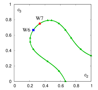
Figure 1: The Williamson curve, i.e. the set of values of $c_{2}$ and $c_{3}$ coefficients for which the 3-stage third-order classical RK schemes can be written in the $2N$-storage format. The symbols (triangles, box and circle) correspond to rational solutions. The blue box and the red circle are the schemes that are discussed in more detail later. W6 and W7 labels indicate the original numbering in Ref. [10]. There is a reflection symmetry along the $c_{2}+c_{3}=1$ line.

While almost any point in the plane (except $c_{2}=c_{3}=1/3$) corresponds to a possible 3-stage third-order classical RK coefficient scheme, only the values on the curve correspond to classical RK methods that can be rewritten in the $2N$-storage format, Algorithm 2. The plot shown in Fig. 1 first appeared in [10] therefore we refer to it as the Williamson curve. To find coefficients for a 3-stage third-order $2N$-storage scheme one can proceed in the following way:

• Pick a value of $c_{2}$ in the allowed range.

• Solve Eq. (20) for $c_{3}$ and pick one of the branches.

• Express all $a_{ij}$, $b_{i}$ coefficients in terms of $c_{2}$ and $c_{3}$ using Eqs. (44)–(49).

• Find $A_{i}$, $B_{i}$ by inverting the relations given in Eqs. (16), (19).

The symbols on the Williamson curve are the points where $c_{2}$ and $c_{3}$ (and all the other coefficients) have rational values. These values are summarized in Table 2 in B. The schemes labeled with the blue box and red circle in the figure play special role in our discussion later. We denote them:

• RK3W6: $c_{2}=1/4$, $c_{3}=2/3$,

• RK3W7: $c_{2}=1/3$, $c_{3}=3/4$,

where “RK3” means that the method is of the third order of global accuracy and “W6” and “W7” preserve the numbering used in [10] where these $2N$-storage schemes first appeared.

For $2N$-storage schemes with more than three stages and orders higher than three there are no analytic solutions available. The coefficients can be found by expressing the order conditions through the coefficients $A_{i}$, $B_{i}$ and solving the resulting system of non-linear equations numerically. Multiple $2N$-storage schemes have been designed in this way in the literature [13, 14, 15, 16, 17, 18, 19, 20].

3.2 Variable step size methods

In the previous sections we considered integration methods that operate with fixed step size. If an estimate of the local error is available one can adjust the step size during the integration. Methods with such a property are known as variable step size or adaptive integrators. To construct a variable step size method one uses two schemes of different order simultaneously. The difference between the two solutions after one step of integration serves as an estimate of the local error and is used to adjust the step size.

Later in Sec. 5.2 we will consider two variable step size schemes where a third-order integrator is used for propagating the solution and an embedded second-order integrator is used to construct an alternative estimate of the solution. Let $d$ be some measure of distance between the solutions (the precise metric used is not important at this point) after the current integration step and $\delta$ a fixed parameter – local tolerance. After an integration step the step size is adjusted as

$$h\to 0.95\sqrt[3]{\frac{\delta}{d}}\,h.$$ (21)

If $d>\delta$ then the integration step is redone with the adjusted $h$. Otherwise the integration proceeds with the adjusted $h$. Such a procedure ensures that the local error at every step is bounded by $\delta$.

It is important to note that setting a bound on the local error does not actually tell one what value of the global error will be achieved. We discuss this point in more detail in Sec. 5.2.

4 Lie group integrators

Consider now a differential equation on a manifold:

$$\frac{dY}{dt}=F(Y)Y.$$ (22)

The results in this section are valid in general for $Y$ taking values on an arbitrary manifold equipped with a group action. For the main discussion that follows, $Y$ will represent a gauge link variable, which is an $\mbox{{SU}}(3)$ matrix. Capital letters are used here to emphasize that the variables do not necessarily commute, unlike in the classical RK case.

If one uses a classical RK scheme for solving Eq. (22) numerically, an update of the form $Y+Const\cdot hF(Y)Y$ will move $Y$ away from the manifold. One needs to use geometric, or structure-preserving integration schemes that update $Y$ as $\exp(Const\cdot hF(Y))Y$. We discuss the two main approaches to constructing such methods next.

4.1 Munthe-Kaas Lie group methods

Let us first return to the classical RK Algorithm 1. One can modify the step 2 in the following way: Evaluate the sum in the second term, exponentiate it and act on $y_{t}$, i.e. $Y_{i}=\exp(h\sum_{j=1}^{i-1}a_{ij}K_{j})Y_{t}$, where $K_{j}=F(Y_{j})$. In this case, however, the extra uncanceled terms in the Taylor expansion of the scheme will result in a method whose global order of accuracy is lower than for the classical scheme. This can be cured by adding commutators. A scheme given in Algorithm 3 which is referred to as the Runge-Kutta-Munthe-Kaas (RKMK) method was introduced in Ref. [21]. There, the expansion of the inverse derivative of the matrix exponential $d\exp_{\cal U}^{-1}({\cal V})$ is truncated at the order $p-1$ (to distinguish it from the full series it is commonly denoted “dexpinv”):

$${\rm dexpinv}({\cal U},{\cal V},p)=\sum_{k=0}^{p-1}\frac{B_{k}}{k!}{\rm ad}_{\cal U}^{k}({\cal V}),$$ (23)

$B_{k}$ are the Bernoulli numbers and the $k$-th power of the adjoint operator ${\rm ad}_{\cal U}({\cal V})$ is given by an iterated commutator application:

$${\rm ad}_{\cal U}^{0}({\cal V}) = {\cal V},$$ (24)

$${\rm ad}_{\cal U}^{1}({\cal V}) = [{\cal U},{\cal V}],$$ (25)

$${\rm ad}_{\cal U}^{k}({\cal V}) = {\rm ad}_{\cal U}({\rm ad}_{\cal U}^{k-1}({\cal V}))$$ (26)

$$= [{\cal U},[{\cal U},[\dots,[{\cal U},{\cal V}]]]].$$

This algorithm results in a Lie group integrator of order $p$ whose coefficients are the coefficients of a classical RK method of order $p$.

Algorithm 3 $s$-stage Runge-Kutta-Munthe-Kaas Lie group method

1:for i=1,…,s do

2:     ${\cal U}_{i}=h\sum_{j=1}^{i-1}a_{ij}\tilde{K}_{j}$$\triangleright$ $a_{i,j\geqslant i}=0$

3:     $Y_{i}=\exp({\cal U}_{i})Y_{t}$

4:     $K_{i}=F(Y_{i})$

5:     $\tilde{K}_{i}={\rm dexpinv}({\cal U}_{i},K_{i},p)$

6:end for

7:${\cal V}=\sum_{i=1}^{s}b_{i}\tilde{K}_{i}$

8:$Y_{t+h}=\exp({\cal V})Y_{t}$

The advantage of Algorithm 3 is that any classical RK method can be turned into a Lie group integrator. The number of commutators can often be reduced as discussed in [22]. It was found, however, that schemes that avoid commutators can be more stable and provide lower global error at the same computational cost. We discuss them next.

4.2 Commutator-free Lie group methods

The earlier work on manifold integrators [23] was extended in Ref. [24] to design a class of commutator-free Lie group methods where each stage of the method may include a composition of several exponentials. A general scheme is given in Algorithm 4. We use the notation of Ref. [4] instead of the original notation of Ref. [24]. $L_{i}$ is the number of exponentials used at stage $i$, $J_{il}$ is the number of right hand side evaluations $K_{j}$ used in the $l$-th exponential at stage $i$, $L$ is the number of exponentials at the final step, and $I_{l}$ is the number of right hand side evaluations $K_{i}$ used in the $l$-th exponential at the final step. ${\cal T}$ represents a “time-ordered” product meaning that an exponential with a lower value of index $l$ is located to the right.

Algorithm 4 $s$-stage commutator-free Lie group method

1:$Y_{1}=Y_{t}$, $K_{1}=F(Y_{1})$

2:for i=2,…,s do

3:     $Y_{i}={\cal T}\left\{\prod_{l=1}^{L_{i}}\exp\left(h\sum_{j=1}^{J_{il}}\alpha_{l;ij}K_{j}\right)\right\}Y_{t}$

4:     $K_{i}=F(Y_{i})$

5:end for

6:$Y_{t+h}={\cal T}\left\{\prod_{l=1}^{L}\exp\left(h\sum_{i=1}^{I_{l}}\beta_{l;i}K_{i}\right)\right\}Y_{t}$

The coefficients $\alpha_{l;ij}$, $\beta_{l;i}$ are related to the coefficients of a classical RK method as [24]

$$\sum_{l=1}^{L_{i}}\alpha_{l;ij}=a_{ij},\,\,\,\,\,\,\sum_{l=1}^{L}\beta_{l;i}=b_{i}.$$ (27)

To better understand the notation of Algorithm 4 we list in Algorithm 5 explicit steps of one of the methods of Ref. [24] where $s=3$, $L_{1}=0$, $L_{2}=1$, $J_{21}=1$, $L_{3}=1$, $J_{31}=2$, $L=2$, $I_{1}=1$ and $I_{2}=3$

Algorithm 5 $3$-stage third-order commutator-free Lie group method of Ref. [24]

1:$Y_{1}=Y_{t}$

2:$K_{1}=F(Y_{1})$

3:$Y_{2}=\exp(h\alpha_{1;21}K_{1})Y_{t}$

4:$K_{2}=F(Y_{2})$

5:$Y_{3}=\exp(h(\alpha_{1;32}K_{2}+\alpha_{1;31}K_{1}))Y_{t}$

6:$K_{3}=F(Y_{3})$

7:$Y_{t+h}=\exp(h(\beta_{2;3}K_{3}+\beta_{2;2}K_{2}+\beta_{2;1}K_{1}))\exp(h\beta_{1;1}K_{1})Y_{t}$

It was found in Ref. [24] that fixing $\beta_{1;1}=\alpha_{1;21}=1/3$ allows one to reuse $Y_{2}$ at the final step and the other coefficients form a one-parameter family of solutions.

4.3 Low-storage commutator-free Lie group methods

Ref. [24] considered such commutator-free methods that reuse exponentials. For instance, in Algorithm 5 $Y_{2}$ is reused at the final stage so one needs only three exponential evaluations in total. Recently, Ref. [4] considered designing a commutator-free method where every next stage reuses $Y_{i}$ from the previous stage and contains only one exponential evaluation per stage (inspired by Algorithm 7 of Ref. [2], see below). Such methods form a subclass of methods of Ref. [24] but differ from the solutions found there by how the exponentials are reused. It turned out that for a 3-stage third-order commutator-free Lie group method with exponential reuse the additional order condition resulting from non-commutativity is the same as the order condition for a $2N$-storage 3-stage third-order classical RK method, Eq. (20). Thus, it was proven in [4] that all $2N$-storage 3-stage third-order classical RK methods of [10], i.e. all points on the Williamson curve, Fig. 1, are also low-storage third-order commutator-free Lie group integrators. It was conjectured in [4] that $2N$-storage classical RK methods of order higher than three are also automatically Lie group integrators of the same order. Numerical evidence was provided in support of the conjecture. Moreover, for a given set of numerical values of coefficients $A_{i}$, $B_{i}$ of a classical $2N$-storage RK method the order of the Lie group method based on it can be determined algorithmically by using B-series [25]. Thus for all such methods that we use here, given the coefficients $A_{i}$, $B_{i}$ of a classical $2N$-storage RK method with $s$ stages and global order of accuracy $p$, the procedure listed in Algorithm 6 is a low-storage commutator-free Lie group method of order $p$.

Algorithm 6 $2N$-storage $s$-stage commutator-free Runge-Kutta Lie group method

1:$Y_{0}=Y_{t}$

2:for i=1,…,s do

3:     $\Delta Y_{i}=A_{i}\Delta Y_{i-1}+hF(Y_{i-1})$$\triangleright$ $A_{1}=0$

4:     $Y_{i}=\exp(B_{i}\Delta Y_{i})Y_{i-1}$

5:end for

6:$Y_{t+h}=Y_{s}$

Let us now turn to the discussion of the integrator first introduced by Lüscher in Ref. [2]. In our notation it is given in Algorithm 7. This scheme belongs to the generic class of commutator-free Lie group methods developed in Ref. [24], however, it differs from the classes of solutions found there. Given that the linear combination of $K_{1}$ and $K_{2}$ is the same at steps 5 and 7 and the previous stage is reused at steps 3, 5 and 7, this integrator has certain reusability property. As far as we are aware, an integrator with the structure and numerical coefficients of Algorithm 7 was not present in the literature on manifold integrators prior to Ref. [2]. Thus, we believe that this method was derived independently. Since its derivation was not presented in [2], we present our derivation in C for illustrative purposes and also to document the order conditions in the form that we were not able to find in the existing literature. This scheme provides a link to the recent developments of Ref. [4].

Algorithm 7 3-stage third-order Lie group method of Ref. [2]

1:$Y_{1}=Y_{t}$

2:$K_{1}=F(Y_{1})$

3:$Y_{2}=\exp\left(h\frac{1}{4}K_{1}\right)Y_{1}$

4:$K_{2}=F(Y_{2})$

5:$Y_{3}=\exp\left(h\left(\frac{8}{9}K_{2}-\frac{17}{36}K_{1}\right)\right)Y_{2}$

6:$K_{3}=F(Y_{3})$

7:$Y_{t+h}=\exp\left(h\left(\frac{3}{4}K_{3}-\frac{8}{9}K_{2}+\frac{17}{36}K_{1}\right)\right)Y_{3}$

It turns out that when Algorithm 7 is rewritten in the $2N$-storage format of Algorithm 6 and the $A_{i}$, $B_{i}$ coefficients are converted to the coefficients of the classical underlying RK scheme, Eqs. (16), (19), the latter are the same as for the RK3W6 classical RK method discussed in Sec. 3.1. It is shown as a blue square on the Williamson curve, Fig. 1. Thus, the method of Ref. [2] belongs to the class of $2N$-storage classical RK methods which are automatically Lie group integrators of the same order as proven in [4]. We will explore this to find the optimal set of coefficients for integrating the gradient flow in Sec. 5.1.

5 Numerical results

To explore the properties of different integrators we used three gauge ensembles with the lattice spacing ranging from $0.15$ fm down to $0.09$ fm listed in Table 1. These ensembles were generated by the MILC collaboration with the one-loop improved gauge action [5] and the Highly Improved Staggered Quark (HISQ) action [26, 27]. The light quark masses were tuned to produce the Goldstone pion mass of about $300$ MeV and the strange and charm quark masses are set to the physical values.

Table 1: The MILC 2+1+1 flavor ensembles used in this study, the details can be found in [28]. In the second column the volume is listed, in the third the approximate lattice spacing and in the fourth the maximum flow time $T_{max}$. Here $T_{max}$ is dimensionless and approximately equal to $(w_{0}^{phys}/a)^{2}$.

Ensemble	$N_{\sigma}^{3}\times N_{\tau}$	$a$, fm	$T_{max}$
l1648f211b580m013m065m838	$16^{3}\times 48$	$0.15$	$1.4$
l2464f211b600m0102m0509m635	$24^{3}\times 64$	$0.12$	$2.0$
l3296f211b630m0074m037m440	$32^{3}\times 96$	$0.09$	$3.8$

We integrate the flow for the amount of time $T_{max}$ that is needed to determine the $w_{0}$-scale according to Eq. (8) with $Const=0.3$. The values of $T_{max}$ for each ensemble are given in Table 1. The $w_{0}$-scale for these ensembles was determined in [29].

To find the global error for each integration method we need to compare to the exact solution. For this purpose we have also implemented a 13-stage eighth-order RK integrator of Munthe-Kaas type, Algorithm 3, with Prince-Dormand coefficients [30] that we refer to as RKMK8. At step size $h=10^{-2}$ it provides the result that is exact within the floating point double precision. For this reason the results from RKMK8 are labeled as “exact.”

To evaluate the global error introduced by the integration methods several quantities are studied. Let us first define the squared distance between two $\mbox{{SU}}(3)$ matrices $X$, $Y$:

$${\cal D}(X,Y)\equiv\sum_{i,j=1}^{3}|X_{ij}-Y_{ij}|^{2}.$$ (28)

For a set of flowed gauge fields the distance from the exact solution is defined as :

$$\Delta V\equiv\sum_{x}\sum_{\mu}\sqrt{{\cal D}(V_{x,\,\mu}(t=T_{max}),V^{exact}_{x,\,\mu}(t=T_{max}))}.$$ (29)

We also calculate the value of the plaquette, rectangle and clover expression averaged over the lattice:

$${\cal P} = \frac{1}{6N_{\sigma}^{3}N_{\tau}}\sum_{x}\sum_{\mu<\nu}{\rm Re}{\rm Tr}(P_{x,\,\mu\nu}),$$ (30)

$${\cal R} = \frac{1}{12N_{\sigma}^{3}N_{\tau}}\sum_{x}\sum_{\mu\neq\nu}{\rm Re}{\rm Tr}(R_{x,\,\mu\nu}),$$ (31)

$${\cal C} = \frac{1}{N_{\sigma}^{3}N_{\tau}}\sum_{x}\sum_{\mu\neq\nu}{\rm Re}{\rm Tr}(C_{x,\,\mu\nu}C_{x,\,\mu\nu}).$$ (32)

Up to a constant prefactor and a shift these quantities provide the three different discretizations of the action, Eqs. (4)–(6) that can be used for the $w_{0}$-scale determination in (8). The global error is also estimated from the differences:

$$\Delta Z\equiv Z(t)-Z^{exact}(t),$$ (33)

where $Z={\cal P}$, ${\cal R}$ or ${\cal C}$ and $t$-dependence means that these quantities are computed using evolved gauge links $V(t)$.

5.1 Tuning the third-order low-storage Lie group integrator

We now address the question of what integrator out of the family of schemes along the Williamson curve can provide the lowest error for integrating the $\mbox{{SU}}(3)$ gradient flow. The Williamson curve is parametrized with a variable $u$ which is the distance along the curve from the point $(2/3,0)$ to $(1,1/3)$ such that $u\in[0,1]$. We pick 32 coefficient schemes $c_{2}(u)$, $c_{3}(u)$ and use their coefficients for low-storage commutator-free Lie group integrators in the form of Algorithm 6. We refer to these methods in general as LSCFRK3 – low-storage, commutator-free, Runge-Kutta, third-order. We picked such values of $c_{2}$ and $c_{3}$ that are either rational or given in terms of radicals. Two particular schemes are of interest in the following: LSCFRK3W6 (equivalent to the integrator of Ref. [2]) and LSCFRK3W7. These are commutator-free Lie group versions of the classical RK integration schemes RK3W6 and RK3W7 discussed in Sec. 3.1.

For this part of the calculation we have chosen 11 lattices per each ensemble separated by 500 molecular dynamics time units for the first two ensembles and 360 time units for the third ensemble in Table 1. For the first two ensembles we ran both the Wilson and Symanzik flow, and only the Symanzik flow for the third ensemble. We ran all 32 LSCFRK3 methods at step sizes $h=1/16$, $1/32$, $1/64$ and $1/128$ and RKMK8 at $h=1/128$.

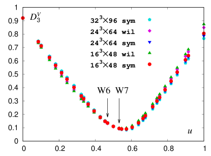
Figure 2: The leading-order coefficient $D_{3}^{V}$ for the global integration error defined in Eq. (34) as function of the distance along the Williamson curve $u$. $u=0$ represents the LSCFRK3 method with $c_{2}=2/3$, $c_{3}=0$, and $u=1$ the method with $c_{2}=1$, $c_{3}=1/3$. The arrows labeled “W6” and “W7” represent the LSCFRK3W6 and LSCFRK3W7 schemes discussed in the text. The statistical errors are (much) smaller than the symbol size.

We first consider the behavior of the distance metric defined in (29). For a third-order method the distance is expected to scale as $O(h^{3})$. We fit the distance $\Delta V$ as a function of the step size to a polynomial form:

$$\langle\Delta V(h)\rangle=D_{3}^{V}h^{3}+D_{4}^{V}h^{4}+D_{5}^{V}h^{5},$$ (34)

where $\langle\dots\rangle$ represents the ensemble average. In some cases we omitted the fifth-order term if a reasonable fit resulted from just the first two terms. The errors on the fit parameters were estimated with a single elimination jackknife procedure.

In Fig. 2 we show the dependence of the leading-order global error coefficient $D_{3}^{V}$ as function of the distance $u$ along the Williamson curve (i.e. the RK coefficient scheme) for all ensembles and flows that we analyzed. The values of $D_{3}^{V}$ are normalized in the following way. For the Symanzik flow on the $16^{3}\times 48$ lattice $D_{3}^{V}(u)$ is divided by $5\times 10^{6}$. (This large factor stems from the fact that our definition of $\Delta V$ is extensive.) For all the other ensembles and flows $D_{3}^{V}(u)$ is divided by such a constant that $D_{3}^{V}(u=0)$ coincides with the one for the $16^{3}\times 48$ lattice Symanzik flow. As one can observe from Fig. 2, the behavior of $D_{3}^{V}(u)$ is similar for different ensembles and different types of flow. The LSCFRK3W7 Lie group integrator is closer to the minimum of the global error than the LSCFRK3W6 method. Note that since the definition of $\Delta V$ is manifestly positive, the leading order coefficient $D_{3}^{V}(u)$ is also positive for all $u$.

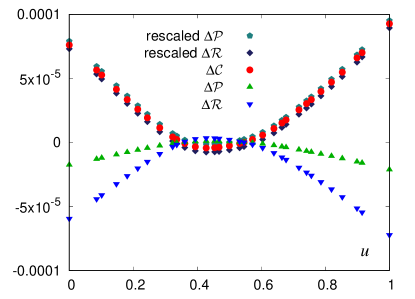
Figure 3: The global integration error in the plaquette $\langle\Delta{\cal P}\rangle$, rectangle $\langle\Delta{\cal R}\rangle$ and the clover expression $\langle\Delta{\cal C}\rangle$ as function of distance along the Williamson curve $u$. $\langle\Delta{\cal P}\rangle$ and $\langle\Delta{\cal R}\rangle$ match $\langle\Delta{\cal C}\rangle$ after they are multiplied by a constant factor. The rescaled values of $\langle\Delta{\cal P}\rangle$ and $\langle\Delta{\cal R}\rangle$ are shifted by $\pm 3\times 10^{-6}$ to be distinguishable from $\langle\Delta{\cal C}\rangle$.

Next, we study the action related observables, Eqs. (30)–(32). In Fig. 3 we show the global errors $\langle\Delta{\cal P}\rangle$, $\langle\Delta{\cal R}\rangle$ and $\langle\Delta{\cal C}\rangle$, defined in (33), as function of $u$ evaluated at $T_{max}=1.4$ with step size $h=1/16$ for the Wilson flow on the $a=0.15$ fm ensemble. When $\langle\Delta{\cal P}\rangle$ and $\langle\Delta{\cal R}\rangle$ are rescaled by a constant so that they coincide with $\langle\Delta{\cal C}\rangle$ at $u=0$, all three quantities collapse onto the same curve. In fact, the collapse is so accurate that the quantities labeled “rescaled” in the figure would be completely covered by the clover $\langle\Delta{\cal C}\rangle$ had not we shifted them by $\pm 3\times 10^{-6}$. This is expected since at later flow times the gauge fields are smooth and the difference between different discretizations diminishes. It is remarkable that the collapse happens already at our coarsest lattice, for the least improved flow at the largest step size, $h=1/16$. We therefore focus solely on the clover discretization in the following.

Similarly to Eq. (34) we fit the global integration error $\Delta{\cal C}$ as function of step size to a polynomial:

$$\langle\Delta{\cal C}(h)\rangle=D_{3}^{C}h^{3}+D_{4}^{C}h^{4}+D_{5}^{C}h^{5}.$$ (35)

We omit the fifth-order term whenever a reasonable fit is obtained with the first two terms.

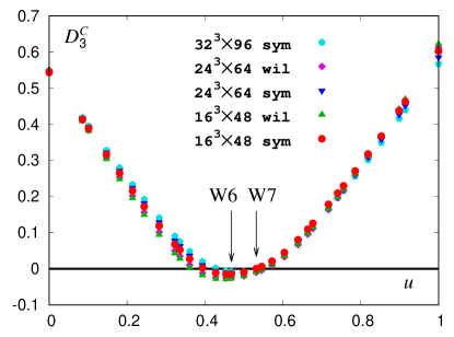
Figure 4: The leading-order coefficient $D_{3}^{C}$ for the global integration error defined in Eq. (35) as function of the distance along the Williamson curve $u$. The arrows labeled “W6” and “W7” represent the LSCFRK3W6 and LSCFRK3W7 schemes discussed in the text. The statistical errors are (much) smaller than the symbol size.

In Fig. 4 we plot the dependence of the leading order global error coefficient $D_{3}^{C}$ as function of $u$ for all ensembles and flows, similar to Fig. 2. The data is rescaled such that all values at $u=0$ match the value of $D_{3}^{C}$ for the Symanzik flow on the $16^{3}\times 48$ lattice. Interestingly, unlike $\langle\Delta V(h)\rangle$, $\langle\Delta{\cal C}(h)\rangle$ is not necessarily positive. We observe that while most of the integration schemes approach the exact result from above, there is a region of $u$ where the exact result is approached from below. The LSCFRK3W7 scheme is close to the point where $D_{3}^{C}=0$ universally across the ensembles and types of flow.

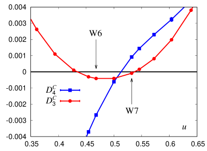
Figure 5: The leading $D_{3}^{C}$ and the next-to-leading order $D_{4}^{C}$ coefficients for the global integration error defined in Eq. (35) for the Symanzik flow on $32^{3}\times 96$ ensemble. The lines are not fits but are drawn to guide the eye. The $D_{4}^{C}$ coefficient is divided by a factor of two to better fit in the frame.

The interval $u\in[0.35,0.65]$ is magnified in Fig. 5 for the $32^{3}\times 96$ ensemble and the Symanzik flow. The fourth-order coefficient $D_{4}^{C}(u)$ is also shown. For the LSCFRK3W7 scheme it is also relatively small. Therefore this method provides close to the lowest error for the action observables that are central for scale setting.

In Fig. 6 we directly compare $\langle\Delta{\cal C}(h)\rangle$ for LSCFRK3W6, LSCFRK3W7 and LSCFRK3W9 for the $32^{3}\times 96$ ensemble. The LSCFRK3W7 scheme has the smallest error $\langle\Delta{\cal C}(h)\rangle$, which due to the competition between the $h^{3}$ and $h^{4}$ terms crosses zero, as shown in the inset of Fig. 6.

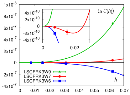
Figure 6: The dependence of the global integration error in the clover expression $\langle\Delta{\cal C}(h)\rangle$ on the step size $h$ for three LSCFRK3 methods. Lines are fits to the data, Eq. (35). For the LSCFRK3W7 method the error changes sign, as shown in the inset.

To summarize, we expect that the LSCFRK3W7 integrator is close to optimal for integrating the gradient flow: it has close to the lowest global error for the gauge fields, Fig. 2, and its leading-order error coefficient $D_{3}^{C}$ is close to 0 for the action related observables, giving much smaller global error, Fig. 6. Moreover, we observe that these properties of LSCFRK3W7 are stable against fluctuations within the gauge ensemble, different ensembles, different types of flow and different discretizations of the observable.

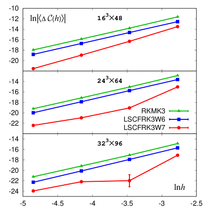
Figure 7: Scaling of the global integration error in the clover observable $\langle\Delta{\cal C}(h)\rangle$ with the step size $h=1/128$, $1/64$, $1/32$ and $1/16$ for the Symanzik flow on the three gauge ensembles. The three third-order methods are discussed in the text. The lines are drawn to guide the eye.

In the following we consider only the Symanzik flow and the clover expression for the observable. The flow is integrated with LSCFRK3W6 and LSCFRK3W7 on 100 lattices that are separated by 50 time units for the first two ensembles and 36 time units for the third in Table 1. The RKMK8 method with $h=10^{-2}$ is used to get the exact solution. The error bars are calculated with respect to 20 jackknife bins. For comparison we also implemented a third-order algorithm of Munthe-Kaas type with Ralston coefficients, Algorithm 3, that we refer to as RKMK3. The results for the global integration error for the clover expression as function of step size $h$ for the three third-order methods are shown in Fig. 7.

It is customary to plot the logarithm of the absolute value of the error vs the logarithm of the step size since the slope then is equal to the order of the method. It also allows one to display the scaling for different integrators that would be too small on the linear scale. This works well when the error is dominated by the leading order term. As we observe in Figs. 5, 6, the LSCFRK3W7 error crosses zero which translates to $-\infty$ on the log-log plot. This explains the non-monotonicity of the LSCFRK3W7 data in Fig. 7. The point with the largest error bar for the $32^{3}\times 96$ lattice is close to the zero crossing and thus the jackknife propagated error bars in $\ln|\Delta{\cal C}|$ are large there. This is expected when the leading-order coefficient is small and the leading term is comparable with the next-to-leading order term for a range of step sizes. For the $16^{3}\times 48$ lattice the $D_{3}^{C}$ coefficient is so close to zero that the error scales almost as $h^{4}$ rather than $h^{3}$. At small enough $h$ all LSCFRK3 methods should approach the expected $h^{3}$ behavior.

In Fig. 7 one can observe that the LSCFRK3W7 method has lower global error than the original integrator of Ref. [2], LSCFRK3W6. The RKMK3 method has the largest error, despite the fact that its coefficients are chosen to be the ones that give the lowest theoretical bound on the global error [31].

The most expensive part of the calculation is evaluation of the right hand side $F(Y)$, Eq. (22). All three methods require three evaluations and thus the same computational cost. (We neglect the fact that the RKMK3 method also requires computation of commutators. In a parallel code that operation is local and thus its overhead is unnoticeable compared with the computation of $F(Y)$, which requires communication.) We conclude that LSCFRK3W7 is the most beneficial Lie group integrator for the gradient flow among the third-order explicit RK methods that we studied.

5.2 Properties of two third-order variable step size integrators

Variable step size integrators were used for gradient flow in Refs. [32, 33], and we also explore methods of this type here for comparison. In Ref. [32] a second-order method was embedded into the LSCFRK3W6 scheme. Methods of this type can be built for all LSCFRK3 schemes so we consider the most generic case. To connect with the form presented in [32] it is convenient to start with the form where $K_{1}$, $K_{2}$ and $K_{3}$ are separated, Algorithm 9 in C. Once the third-order integrator stages are complete and all $K_{i}$ are computed, another stage is performed to get a lower order estimate:

$$\tilde{Y}_{t+h}=\exp(h(\lambda_{3}K_{3}+\lambda_{2}K_{2}+\lambda_{1}K_{1}))Y_{t}.$$ (36)

For $\tilde{Y}_{t+h}$ to be globally second order (and locally third order) the coefficients $\lambda_{i}$ need to satisfy the following conditions:

$$\lambda_{1}+\lambda_{2}+\lambda_{3} = 1,$$ (37)

$$c_{2}\lambda_{2}+c_{3}\lambda_{3} = \frac{1}{2}.$$ (38)

For any LSCFRK3 method determined by $c_{2}(u)$, $c_{3}(u)$ there is a one-parameter family of embedded second-order methods. The variable step size scheme is no longer a low-storage method since $K_{i}$ need to be stored separately for the stage (36) to be applied.

For the measure of the local error Ref. [32] suggested

$$d=\max_{x,\mu}\frac{1}{9}\sqrt{{\cal D}(V_{x,\,\mu}(t+h),\tilde{V}_{x,\,\mu}(t+h))}.$$ (39)

The full method is summarized in Algorithm 8 (the local tolerance $\delta$ is a preset parameter).

Algorithm 8 4-stage third-order commutator-free variable step size Lie group method

1:Perform the three stages of Algorithm 9 for each gauge link to get $V_{x,\,\mu}(t+h)$.

2:Store $K_{i}$, $i=1,\dots,3$.

3:Compute $\tilde{V}_{x,\,\mu}(t+h)$ using Eq. (36).

4:Compute the maximum distance $d$ with Eq. (39).

5:Set $h\to 0.95\sqrt[3]{\frac{\delta}{d}}\,h$.

6:If $d>\delta$ restart from step 1.

We take $\lambda_{3}$ as a free parameter (this fixes $\lambda_{1}$ and $\lambda_{2}$) and test two variable step size methods based on $W6$ (as in [32]) and $W7$ coefficients. These methods are referred to as CFRK3W6VS and CFRK3W7VS in the following (VS = variable step size). The tests are performed on a single $16^{3}\times 48$ lattice with the Symanzik flow to illustrate a qualitative point.

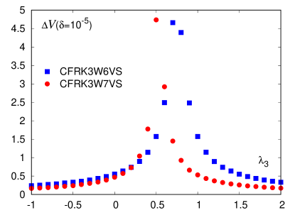
Figure 8: The global integration error for gauge fields defined in Eq. (29) as function of the parameter $\lambda_{3}$ that distinguishes variable step size methods. The CFRK3W6VS and CFRK3W7VS methods differ in what third-order integrator is used. The global error is evaluated at the same local tolerance $\delta=10^{-5}$ for all methods. The results are from the flow on a single $16^{3}\times 48$ lattice and therefore have no errorbars.

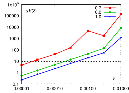
Figure 9: The global integration error $\Delta V(\delta)$ as function of the local tolerance $\delta$ for the three third-order variable step size methods CFRK3W6VS($\lambda_{3}$) for $\lambda_{3}=-1$, $0$ and $0.7$. The results are from the flow on a single $16^{3}\times 48$ lattice and therefore have no errorbars.

For a set of local tolerances $\delta=10^{-5}$, $3\times 10^{-5}$, $10^{-4}$, $3\times 10^{-4}$, $10^{-3}$, $3\times 10^{-3}$ and $10^{-2}$ CFRK3W6VS and CFRK3W7VS were run for values of $\lambda_{3}\in[-1,2]$ separated by $0.1$. The results for the global error in the gauge fields $\Delta V(\delta)$ defined in (29) are shown in Fig. 8 for a fixed value of tolerance $\delta=10^{-5}$ as function of the $\lambda_{3}$ parameter. There seems to be some room for tuning $\lambda_{3}$ since there is a significant difference in what global error is achieved by different methods. In Fig. 9 the dependence of the global error $\Delta V(\delta)$ on the local tolerance $\delta$ is shown for the three CFRK3W6VS methods with $\lambda_{3}=-1$, $0$ and $0.7$. Note that $\lambda_{3}=0$ corresponds to the variable step size method of Ref. [32]. $\lambda_{3}=0.7$ gives the highest error among the CFRK3W6VS schemes shown in Fig. 8. It may seem that $\lambda_{3}=-1$ is the best method.

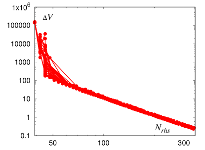
Figure 10: The global error $\Delta V$ as function of the number of right hand side evaluations of Eq. (7) for all 62 variable step size schemes shown in Fig. 8. The results are from the flow on a single $16^{3}\times 48$ lattice and therefore have no errorbars.

However, the relevant question to address is what number of steps (i.e. computational effort) each method needs to reach a certain global error. For this purpose all 62 schemes shown in Fig. 8 are plotted against the number of right hand side evaluations (which is the number of steps times three stages per step) $N_{rhs}$ in Fig. 10. All schemes collapse on the same line apart from the region of small number of steps at the beginning (large local tolerance) where the subleading corrections to scaling are still large. There is no room for tuning – all methods would reach a given global error with the same computational effort independently of what coefficients of the embedded low-order scheme $\lambda_{i}$ are used. What is different for different schemes is the value of the local tolerance at which that global error is achieved. For instance, the CFRK3W6VS with $\lambda_{3}=0.7$ achieves the global error $\Delta V=10$ at the local tolerance $\delta=2.2\times 10^{-5}$, with $\lambda_{3}=0$ at $\delta=2\times 10^{-4}$ and with $\lambda_{3}=-1$ at $\delta=4.5\times 10^{-4}$, Fig. 9.

This brings us to an important point. It may be tempting, as happens in some literature, to interpret the local tolerance $\delta$ as a universal parameter that can be set once and after that the integrator self-tunes and takes care of the global error. Contrary to that, we observe that there is no apriori way to know what global integration error is achieved for a specific value of $\delta$ on a given lattice ensemble. Therefore, $\delta$ should be treated in the same way as the step size $h$ in fixed step size methods. For a calculation performed at a single value of $h$ there is no way to estimate what global error was achieved, apart from knowing that it is proportional to $h^{p}$, where $p$ is the order of the method. One needs to either calculate the exact (or high-precision) solution and compare with it, or perform the calculation at several step sizes, study the dependence of the error in the observable of interest on the step size and decide what step size is appropriate for a given lattice ensemble. Similarly, one needs to study the scaling of the error with respect to $\delta$ and pick $\delta$ based on that. It will certainly be different for each problem, since the numerical value of the global integration error is influenced by many factors such as the integration method, what gauge ensembles are used, type of the gradient flow, for how long the flow is run, etc.

Given that all embedded methods are equivalent with respect to the computational cost for a given higher-order scheme and we do not observe a significant difference between CFRK3W6VS and CFRK3W7VS, we only perform calculations with the original method of Ref. [32] which is CFRK3W6VS($\lambda_{3}=0$).

For comparison we also implemented the Bogacki-Shampine variable step size integrator [34] that was used for gradient flow in Ref. [33]. The Lie group integrator of this type is built as an extension of the RKMK3 method (i.e. involves commutators). It requires four right hand side evaluations; however, the last evaluation at the current step is the first on the next, so it can be stored and reused (so called First Same As Last – FSAL property). Therefore in practice it requires only three right hand side evaluations, which is the same computational effort as for all the other third-order methods explored here. Since we do not find this method to be beneficial, we do not list the full algorithm. The details can be found in [34, 33]. This method is referred to as RKMK3BS.

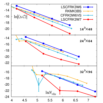
Figure 11: Scaling of the global integration error in the clover observable $\langle\Delta{\cal C}\rangle$ with the number of right hand side evaluations $N_{rhs}$ for the Symanzik flow on the three gauge ensembles. The variable step size methods RKMK3BS and CFRK3W6VS were run with a set of local tolerances $\delta=10^{-6}$, $3\times 10^{-6}$, $10^{-5}$, $3\times 10^{-5}$, $10^{-4}$, $3\times 10^{-4}$, $10^{-3}$, $3\times 10^{-3}$. The data for the fixed step size methods LSCFRK3W6 and LSCFRK3W7 is the same as in Fig. 7. The lines are drawn to guide the eye.

As in Sec. 5.1 the Symanzik flow is measured on 100 lattices from each ensemble of Table 1. The error bars are estimated from 20 jackknife bins. In Fig. 11 the logarithm of the global error $\langle\Delta{\cal C}(h)\rangle$ is shown vs the logarithm of the number of the right hand side evaluations $N_{rhs}$ for the two fixed step size integrators LSCFRK3W6 and LSCFRK3W7 that are discussed in Sec. 5.1 and the two variable step size methods CFRK3W6VS($\lambda_{3}=0$) and RKMK3BS. The origin of the non-monotonic behavior for CFRK3W6VS is similar to the one for LSCFRK3W7 – its global error crosses zero at some value of $\delta$. Interestingly, while both variable step size methods are more beneficial than LSCFRK3W6 for the $16^{3}\times 48$ and $24^{3}\times 64$ ensembles, for the $32^{3}\times 96$ ensemble in the regime where all integrators approach the expected cubic scaling, the variable step size schemes require comparable or larger computational effort than LSCFRK3W6. The fixed step size LSCFRK3W7 method requires the least computational effort for all three ensembles except the region of large local tolerance (small number of right hand side evaluations). We conclude that for the scale setting applications there may be no benefit from using variable step size integrators, at least for the gauge ensembles that we used for this study.

Our findings are in contrast with the studies of Ref. [32] where large computational savings were reported for CFRK3W6VS($\lambda_{3}=0$). However, it appears that there the gradient flow was used in a very different regime. Apart from less important differences in the gauge couplings, boundary conditions and lattice volumes, the flow was run significantly longer to achieve a much larger smoothing radius than is needed for $w_{0}$-scale setting. Translated for the gauge ensembles used in this study the flow would be run in the ranges $T_{max}=2.9-8$ for the $a=0.15$ fm, $T_{max}=6.5-18$ for the $a=0.12$ fm and $T_{max}=11.5-32$ for the $a=0.09$ fm ensembles (compare with $T_{max}$ in Table 1).

5.3 Two low-storage fourth-order Lie group integrators

Reference [4] opened a possibility of building low-storage Lie group integrators from classical $2N$-storage RK methods. There are a number of fourth-order $2N$-storage methods in the literature [13, 14, 15, 16, 17, 18, 19] that were constructed for different applications. Most of them include large number of stages and may therefore be computationally inefficient for integration of the gradient flow in lattice gauge theory.

We study two fourth-order methods that have five (the minimal possible number) [13] and six [15] stages which we refer to as LSCFRK4CK and LSCFRK4BBB, respectively. Their coefficients were found by solving a system of nonlinear equations resulting from eight order conditions for a classical RK method and additional problem-dependent constraints (e.g. increased regions of stability). These coefficients in the $2N$-storage format are listed in B.

As in Sec. 5.1, the tests are performed with the Symanzik flow, clover observable on 100 lattices from the ensembles listed in Table 1. The step sizes $h=1/16$, $1/32$, $1/64$ and $1/128$ are used and the exact solution is obtained with RKMK8 at $h=10^{-2}$. For comparison we also implemented a fourth-order method of Munthe-Kaas type, RKMK4. Such a method was employed in [35]. Our implementation is not exactly the same as there and provides a slightly smaller global error, but our findings are qualitatively similar.

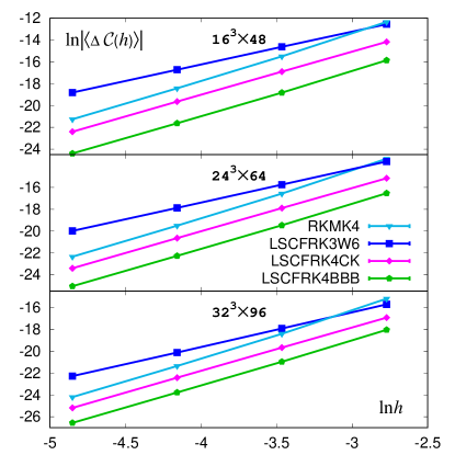
Figure 12: Scaling of the global integration error in the clover observable $\langle\Delta{\cal C}(h)\rangle$ with the step size $h=1/128$, $1/64$, $1/32$ and $1/16$ for the Symanzik flow on the three gauge ensembles. The three fourth-order methods are discussed in the text. The lines are drawn to guide the eye.

The scaling of the error in the clover observable $\ln|\langle\Delta{\cal C}(h)\rangle|$ as function of $\ln h$ is shown in Fig. 12 for the LSCFRK3W6, LSCFRK4CK, LSCFRK4BBB and RKMK4 methods. RKMK4 has the largest error among the fourth-order methods while the lowest global integration error is achieved with LSCFRK4BBB.

The $2N$-storage RK methods with $s$ stages have $2s-1$ parameters ($A_{1}=0$ for explicit methods). Thus, the five-stage LSCFRK4CK integrator also belongs to a one-parameter family since there are 8 classical order conditions at fourth order. There may also be some possibility for tuning that integrator similarly to our discussion in Sec. 5.1. However, due to the complexity of the order conditions, no analytic solutions such as Eq. (20) are available. This makes tuning of that integrator a complicated task. We note that there are three more coefficient schemes reported in Ref. [13], but we found them less efficient than the main scheme that Ref. [13] recommended and which was implemented in this study.

5.4 Final comparison

The integration schemes that we explored differ in the number of stages. To compare their computational efficiency, Fig. 13 shows the dependence of the global error in the clover observable vs the number of right hand side evaluations for the third-order method of Ref. [2] LSCFRK3W6, the third-order scheme LSCFRK3W7 that we discussed in Sec. 5.1, and the two fourth-order methods LSCFRK4CK and LSCFRK4BBB. Compared with LSCFRK3W6 we find that the LSCFRK3W7 scheme produces lower global error at all step sizes explored and is thus more beneficial computationally. The fourth-order LSCFRK4BBB scheme becomes more beneficial than LSCFRK3W6 at step size of about $h=1/16$ for the $16^{3}\times 48$ and $24^{3}\times 64$ ensembles and about $h=1/32$ for the $32^{3}\times 96$ ensemble (the step size here is for the LSCFRK3W6 integrator, the one for LSCFRK4BBB is about twice as large at the crossing point). Compared with LSCFRK3W7, LSCFRK4BBB becomes more efficient at $h=1/128$ ($h$ for LSCFRK3W7). For the $32^{3}\times 96$ ensemble the five-stage LSCFRK4CK method becomes comparable with LSCFRK4BBB.

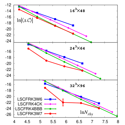
Figure 13: Scaling of the global integration error in the clover observable $\langle\Delta{\cal C}\rangle$ with the number of right hand side evaluations $N_{rhs}$ for the Symanzik flow on the three gauge ensembles. All integrators were run at step sizes $h=1/128$, $1/64$, $1/32$ and $1/16$ except LSCFRK4CK and LSCFRK4BBB where $h=1/8$ was also included. The lines are drawn to guide the eye.

6 Conclusion

Based on the connection [4] between the $2N$-storage classical Runge-Kutta methods [10] and commutator-free integrators [24] we explored several possible improvements in the efficiency of integrating the gradient flow in lattice gauge theory.

Among the low-storage three-stage third-order schemes that are parametrized by the Williamson curve the LSCFRK3W7 is the most promising. Its global error in the norm of the gauge field is close to the minimum, Fig. 2. For the action observables this method is close to the point where the leading order error coefficient is close to zero. Like the originally proposed LSCFRK3W6 method of Lüscher [2], LSCFRK3W7 has rational coefficients that are given in the $2N$-storage form in B. The performance of the LSCFRK3W7 method is universal across ensembles with different lattice spacing, types of flow and types of observable that we explored. For a specific gradient flow application the reader can always revisit the tuning of the third-order scheme similar to our study in Sec. 5.1 by e.g. running a small-scale test on the set of rational values of $c_{2}$ and $c_{3}$ coefficients given in B that reasonably cover the Williamson curve. For the reader’s convenience we also provide a listing of the Mathematica script that calculates the LSCFRK3 method coefficients in various formats from given $c_{2}$ and $c_{3}$ in D.

Our studies of the third-order variable step size methods in Sec. 5.2 indicate that one needs to exercise caution in interpreting the local tolerance $\delta$ parameter. Its relation to the global integration error is not a priori known, in the same way as it happens with the step size $h$ for fixed step size methods. Thus, in both situations one needs to study the scaling of the global error with the control parameter, step size $h$ or local tolerance $\delta$, and tune it based on that for each specific case. For $w_{0}$-scale setting applications we find that it is still computationally more efficient to use the fixed step size LSCFRK3W7 method rather than the third-order variable step size schemes. For applications where the third-order variable step size methods may be beneficial we also include the coefficient scheme that allows one to reuse the second stage of the third-order integrator in the embedded second-order integrator in the Mathematica script in D.

There are two low-storage fourth-order methods studied in Sec. 5.3 that may be well-suited for gradient flow applications. We find that the LSCFRK4BBB method is the most computationally efficient one, although the five-stage LSCFRK4CK method becomes comparable at finer ensembles. For the gauge ensembles that we studied we conclude that if one needs to run the LSCFRK3W6 integrator at time steps lower that $1/32$, it is more beneficial to switch to LSCFRK4BBB. A fourth-order RKMK4 method was used in Ref. [35] to provide a conservative estimate of the integration error for observables related to the topology of gauge fields. We believe that LSCFRK4BBB provides a better alternative to RKMK4, see Fig. 12. For the three gauge ensembles used here the LSCFRK4BBB integrator is stable at the largest step size we tried, $h=1/8$. The average integration error at this step size for the clover observable is $\langle\Delta{\cal C}(h=1/8)\rangle=-3.7\times 10^{-6}$ for the $a=0.15$ fm, $\langle\Delta{\cal C}(h=1/8)\rangle=-1.7\times 10^{-6}$ for the $a=0.12$ fm and $\langle\Delta{\cal C}(h=1/8)\rangle=-3.5\times 10^{-7}$ for the $a=0.09$ fm ensemble.

Based on our findings we recommend LSCFRK3W7, LSCFRK4BBB and LSCFRK4CK for integrating the gradient flow. Exact speedups depend on the accuracy required for the flow observables. For the ensembles we used LSCFRK3W7 is about twice as efficient as LSCFRK3W6 for the $w_{0}$-scale setting. Since these methods are all written in the $2N$-storage format, it is very easy to implement different integrators in the existing code. For instance, in the MILC code [36] the main loop over the stages in Algorithm 6 is the following:

  for( i=0; i<N_stages; i++ ) {
    integrate_RK_2N_one_stage( A_2N[i],
                  -B_2N[i]*stepsize );
  }

The only change required in the code to implement a different LSCFRK integrator is to change the following compile-time parameters: N_stages – the number of stages of the method, and A_2N, B_2N – the values of the two arrays of size N_stages that store the $A_{i}$, $B_{i}$ coefficients in the $2N$-storage format. The code in the integrate_RK_2N_one_stage function performs one stage of Algorithm 6 and is typically already present in the lattice codes that implemented Algorithm 7.

To summarize, we presented several Lie group methods that may provide better computational efficiency for integrating the gradient flow in lattice gauge theory. Given their low-storage properties, they are easy to implement in the existing codes. For the reader interested in exploring the properties and implementation of the low-storage Lie group integrators in a simpler setting we point out that a simple Matlab script for integrating the equation of motion of a rotating free rigid body is included in the Appendix of Ref. [4].

Acknowledgements. We thank the MILC collaboration for sharing the gauge configurations, Oliver Witzel for an independent test of the flow observables, Oswald Knoth for checking the order conditions for the low-storage Lie group integrators used here and Claude Bernard, Steven Gottlieb and Johannes Weber for careful reading and comments on the manuscript. This work was in part supported by the U.S. National Science Foundation under award PHY-1812332.

Appendix A Some order conditions for classical Runge-Kutta methods

The coefficients of a third-order explicit classical Runge-Kutta method satisfy the following order conditions:

$$\sum_{i}b_{i} = 1,$$ (40)

$$\sum_{i}b_{i}c_{i} = \frac{1}{2},$$ (41)

$$\sum_{i}b_{i}c_{i}^{2} = \frac{1}{3},$$ (42)

$$\sum_{i,j}b_{i}a_{ij}c_{j} = \frac{1}{6}.$$ (43)

A 3-stage method has six independent parameters. Picking $c_{2}$ and $c_{3}$ as free parameters one gets the most generic branch of solutions $c_{2}\neq 0\neq c_{3}\neq c_{2}\neq 2/3$ [8]:

$$b_{2} = \frac{3c_{3}-2}{6c_{2}(c_{3}-c_{2})},$$ (44)

$$b_{3} = \frac{2-3c_{2}}{6c_{3}(c_{3}-c_{2})},$$ (45)

$$a_{32} = \frac{c_{3}(c_{3}-c_{2})}{c_{2}(2-3c_{2})},$$ (46)

$$b_{1} = 1-b_{2}-b_{3},$$ (47)

$$a_{21} = c_{2},$$ (48)

$$a_{31} = c_{3}-a_{32}.$$ (49)

Appendix B Coefficients for several $2N$-storage third- and fourth-order classical RK methods

For future reference and possible integrator tuning we list several rational coefficient schemes in Table 2.

Table 2: Three-stage third-order $2N$-storage schemes with rational coefficients. The original numbering of Ref. [10] is listed in the first column. The additional schemes that we found are marked with the asterisk. There are many more than we show here, but as the numerator and denominator grow larger they are not convenient to use.

Numbering [10]	$c_{2}$	$c_{3}$
4	$2/3$	$0$
	$7/12$	$2/15$
	$823/1887$	$153/592$
5	$1/4$	$5/12$
	$1418/6783$	$9894/19285$
	$1418/6783$	$1064/1887$
6	$1/4$	$2/3$
7	$1/3$	$3/4$
	$823/1887$	$5365/6783$
	$9391/19285$	$5365/6783$
	$7/12$	$3/4$
	$439/592$	$1064/1887$
	$13/15$	$5/12$
12	$2/3$	$2/3$
14	$1$	$1/3$

The coefficients of the RK3W6 and RK3W7 schemes in the $2N$-storage format are listed in Table 3 and of the RK4CK and RK4BBB in Table 4. Note that the RK4CK coefficients were found numerically and then close rational expressions were found that provide 26 digits of accuracy. For the RK4BBB method the coefficients are given with 12 digits of accuracy in [15] therefore one cannot expect the error to be below $10^{-12}$. This bound is however well below the typical precision needed in gradient flow applications.

Table 3: The coefficients of the two $2N$-storage third-order schemes of [10] that are the basis for the LSCFRK3W6 and LSCFRK3W7 methods discussed in Sec. 5.1.

Coefficient	RK3W6	RK3W7
$A_{1}$	$0$	$0$
$A_{2}$	$-17/32$	$-5/9$
$A_{3}$	$-32/27$	$-153/128$
$B_{1}$	$1/4$	$1/3$
$B_{2}$	$8/9$	$15/16$
$B_{3}$	$3/4$	$8/15$

Table 4: The coefficients of the two $2N$-storage fourth-order schemes of [13] and [15] that are the basis for the LSCFRK4CK and LSCFRK4BBB methods discussed in Sec. 5.3.

Coefficient	RK4CK
$A_{1}$	$0$
$A_{2}$	$-567301805773/1357537059087$
$A_{3}$	$-2404267990393/2016746695238$
$A_{4}$	$-3550918686646/2091501179385$
$A_{5}$	$-1275806237668/842570457699$
$B_{1}$	$1432997174477/9575080441755$
$B_{2}$	$5161836677717/13612068292357$
$B_{3}$	$1720146321549/2090206949498$
$B_{4}$	$3134564353537/4481467310338$
$B_{5}$	$2277821191437/14882151754819$
Coefficient	RK4BBB
$A_{1}$	$0$
$A_{2}$	$-0.737101392796$
$A_{3}$	$-1.634740794341$
$A_{4}$	$-0.744739003780$
$A_{5}$	$-1.469897351522$
$A_{6}$	$-2.813971388035$
$B_{1}$	$0.032918605146$
$B_{2}$	$0.823256998200$
$B_{3}$	$0.381530948900$
$B_{4}$	$0.200092213184$
$B_{5}$	$1.718581042715$
$B_{6}$	$0.27$

Appendix C Derivation of the Lie group integrator of Ref. [2]

It is illustrative to discuss the properties of the integrator provided by Lüscher in Ref. [2]. As this coefficient scheme was not present in the literature on Lie group methods at the time, we believe that the method was derived independently. Let us start with a generic algorithm that reuses the function value from the previous stage, Algorithm 9, and contains six yet undetermined parameters.

Algorithm 9 3-stage generic Lie group method with reuse of function values

1:$Y_{1}=Y_{t}$

2:$K_{1}=F(Y_{1})$

3:$Y_{2}=\exp\left(h\alpha_{21}K_{1}\right)Y_{1}$

4:$K_{2}=F(Y_{2})$

5:$Y_{3}=\exp\left(h\left(\alpha_{32}K_{2}+\alpha_{31}K_{1}\right)\right)Y_{2}$

6:$K_{3}=F(Y_{3})$

7:$Y_{t+h}=\exp\left(h\left(\beta_{3}K_{3}+\beta_{2}K_{2}+\beta_{1}K_{1}\right)\right)Y_{3}$

8:or

7:$Y_{t+h}=\exp\left(h\left(\beta_{3}K_{3}+c(\alpha_{32}K_{2}+\alpha_{31}K_{1})\right)\right)Y_{3}$ $\triangleright$ See text.

If $Y_{3}$ and $Y_{2}$ are substituted in terms of $Y_{1}$, one can recognize that this scheme belongs to the class of commutator-free Lie group integrators explored in Ref. [24]. However, it does not belong to the classes of solutions found there.

We would like to find a solution of the order conditions that allows for a third-order global accuracy method. For a classical RK method there are four order conditions, thus, we need at least four parameters to satisfy them. For a Lie group integrator of this type we need at least five parameters. This can be seen from the following argument. If we take, for instance, a third-order Crouch-Grossman method [23] (which is a commutator-free Lie group integrator with a more restricted structure than the methods of [24]), there is a non-classical order condition arising from non-commutativity, so there are five in total. If we follow the RKMK route [37, 21], one needs, at least, one commutator for a third-order method. Thus, if we would like to avoid commutators, we need at least one more coefficient to tune to cancel the effect of the commutator. Overall, it may be possible to construct a scheme with five rather than six different parameters. This can be beneficial to reduce the complexity of the order conditions, and also to reuse storage. We can trade $\beta_{1}$ and $\beta_{2}$ for a single coefficient $c$ by requiring:

$$\beta_{1}=c\alpha_{31},\,\,\,\,\,\beta_{2}=c\alpha_{32}.$$ (50)

This way one can store the combination $\alpha_{32}K_{2}+\alpha_{31}K_{1}$, rather than $K_{1}$ and $K_{2}$ separately, overwriting $K_{1}$ with this combination.

As is done for classical RK methods, by Taylor expanding the numerical scheme and comparing with the expansion of the exact solution one arrives at the following order conditions:

$$\phantom{+\frac{1}{2}\beta_{3}(\beta_{3}+c(\alpha_{32}+\alpha_{31}))(\alpha_{32}+\alpha_{31}+\alpha_{21})}\mathllap{\beta_{3}+(1+c)(\alpha_{32}+\alpha_{31})+\alpha_{21}} = 1,$$ (51)

$$\phantom{+\frac{1}{2}\beta_{3}(\beta_{3}+c(\alpha_{32}+\alpha_{31}))(\alpha_{32}+\alpha_{31}+\alpha_{21})}\mathllap{\beta_{3}(\alpha_{32}+\alpha_{31}+\alpha_{21})+(1+c)\alpha_{32}\alpha_{21}} = \frac{1}{2},$$ (52)

$$\phantom{+\frac{1}{2}\beta_{3}(\beta_{3}+c(\alpha_{32}+\alpha_{31}))(\alpha_{32}+\alpha_{31}+\alpha_{21})}\mathllap{\beta_{3}(\alpha_{32}+\alpha_{31}+\alpha_{21})^{2}+(1+c)\alpha_{32}\alpha_{21}^{2}} = \frac{1}{3},$$ (53)

$$\phantom{+\frac{1}{2}\beta_{3}(\beta_{3}+c(\alpha_{32}+\alpha_{31}))(\alpha_{32}+\alpha_{31}+\alpha_{21})}\mathllap{\beta_{3}\alpha_{32}\alpha_{21}} = \frac{1}{6},$$ (54)

$$\frac{3}{2}\left[\beta_{3}(\alpha_{32}+\alpha_{31}+\alpha_{21})^{2}+(1+c)\alpha_{32}\alpha_{21}^{2}\right]$$

$$+\frac{1}{2}\beta_{3}(\beta_{3}+c(\alpha_{32}+\alpha_{31}))(\alpha_{32}+\alpha_{31}+\alpha_{21})$$

$$+\frac{1}{2}[c(\beta_{3}+c(\alpha_{32}+\alpha_{31}))$$

$$+\alpha_{32}+\alpha_{31}]\alpha_{32}\alpha_{21}$$

$$+c(\alpha_{32}+\alpha_{31})\alpha_{32}\alpha_{21} = \frac{1}{2},$$ (55)

$$\phantom{+\frac{1}{2}\beta_{3}(\beta_{3}+c(\alpha_{32}+\alpha_{31}))(\alpha_{32}+\alpha_{31}+\alpha_{21})}\mathllap{\frac{1}{2}\beta_{3}(\beta_{3}+c(\alpha_{32}+\alpha_{31}))(\alpha_{32}+\alpha_{31}+\alpha_{21})}$$

$$+\frac{1}{2}[c(\beta_{3}+c(\alpha_{32}+\alpha_{31}))$$

$$+\alpha_{32}+\alpha_{31}]\alpha_{32}\alpha_{21}$$

$$+(\beta_{3}+c(\alpha_{32}+\alpha_{31}))\alpha_{32}\alpha_{21} = \frac{1}{6}.$$ (56)

Eqs. (51)–(54) are equivalent to the classical order conditions for a third-order scheme, expressed in terms of the coefficients $\alpha_{ij}$, $\beta_{i}$ (their relation to the classical coefficients will become clear in a moment). Eqs. (55), (56) appear when $Y$ is a vector or a matrix and terms $F^{\prime}F^{2}$ and $FF^{\prime}F$ in the Taylor expansion can no longer be combined. By using the four classical order conditions (51)–(54) one finds that the two conditions (55), (56) are not independent and can be condensed into a single condition:

$$\frac{1}{2}\left[\beta_{3}+c(\alpha_{32}+\alpha_{31})\right]+(1+c)(\alpha_{32}+\alpha_{31})\alpha_{32}\alpha_{21}=\frac{1}{6}.$$ (57)

Now there are five unknowns and five (non-linear) equations. As is obvious from Eqs. (51)–(54), (57) this system can become significantly simpler if $1+c=0$, so we can try $c=-1$ as a first guess. Then dividing (53) by (52) we get $\alpha_{32}+\alpha_{31}+\alpha_{21}=2/3$, substituting that into (52) we immediately get $\beta_{3}=3/4$, from (51) $\alpha_{21}=1/4$, from (54) $\alpha_{32}=8/9$, and, finally, $\alpha_{31}=-17/36$. We can check that Eq. (57) is also satisfied. These are nothing else but the coefficients of the scheme of Ref. [2], Algorithm 7.

However, as the reader can verify, there are solutions for other values of $c$. This is possible because, as one can show, in the form involving the coefficient $c$, Eq. (50), the non-classical constraint (57) is a linear combination of (51)–(53). Had we kept $\beta_{1}$ and $\beta_{2}$ as independent coefficients this would not happen. We would still end up with a one-parameter family of solutions (six coefficients with five constraints), but (57) would be linearly independent.

As is now clear from the discussion in Sec. 4.3, the integrator of [2] is, in fact, a low-storage commutator-free Lie group integrator that belongs to the family of schemes based on the classical $2N$-storage methods of Ref. [10]. See [4] for detailed discussion. We call this scheme LSCFRK3W6 in Sec. 5.1. Its set of classical RK coefficients is $a_{21}=1/4$, $a_{31}=-2/9$, $a_{32}=8/9$, $b_{1}=1/4$, $b_{2}=0$, $b_{3}=3/4$ and they are related to the set of $\alpha$’s and $\beta$’s we started with as

$$\alpha_{21} = a_{21},$$ (58)

$$\alpha_{31} = a_{31}-a_{21},$$ (59)

$$\alpha_{32} = a_{32},$$ (60)

$$\beta_{1} = b_{1}-a_{31},$$ (61)

$$\beta_{2} = b_{2}-a_{32},$$ (62)

$$\beta_{3} = b_{3}.$$ (63)

The coefficients in the $2N$-storage format, Algorithm 6, are given in the second column of Table 3.

Appendix D Mathematica script

A Wolfram Mathematica script (tested with version 11) that calculates the coefficients for the $2N$-storage explicit three-stage third-order Runge-Kutta methods from provided $c_{2}$ and $c_{3}$ coefficients is given below. The reader can simply copy and paste it into an empty Mathematica notebook (the formatting will most likely be lost).

(* Note: enclosing parentheses are needed
so that Abort[] function could actually abort
the execution of the cell *)
( (* <---- do not remove *)
(* SET c2 AND c3 HERE e.g. from Table B.2 *)
c2 := 1/4;
c3 := 2/3;

(* check the singular point *)
If[c2 == 1/3 && c3 == 1/3,
Print["No RK scheme with c2=c3=1/3 exists"];
Abort[]];

(* check if low-storage *)
If[c3^2*(1 - c2) + c3*(c2^2 + 1/2*c2 - 1)
+ (1/3 - 1/2*c2) != 0,
Print["c2,c3 -- not a low-storage scheme"];
Abort[]];

(* check if limiting case c2=2/3,c3=0
or c2=c3=2/3 is hit *)

If[c2 == 2/3 && c3 == 0,
b3 := -1/3; b2 := 3/4; b1 := 1/4 - b3;
a32 := 1/4/b3; a31 := -a32; a21 := 2/3,
If[c2 == 2/3 && c3 == 2/3,
b3 := 1/3; b2 := 3/4 - b3; b1 := 1/4;
a32 := 1/4/b3; a31 := 2/3 - a32; a21 := 2/3,
b2 := (3*c3 - 2)/6/c2/(c3 - c2);
b3 := (2 - 3*c2)/6/c3/(c3 - c2);
a32 := c3*(c3 - c2)/c2/(2 - 3*c2);
b1 := 1 - b2 - b3; a31 = c3 - a32; a21 := c2]];

Print["Coefficients in classical RK form:"];
Print["a21=", a21];
Print["a31=", a31];
Print["a32=", a32];
Print["b1=", b1];
Print["b2=", b2];
Print["b3=", b3];

alpha21 := a21;
alpha31 := a31 - a21;
alpha32 := a32;
beta3 := b3;
c := (b1 - a31)/(a31 - a21);

Print["Coefficients in the form of"];
Print["Luescher, 1006.4518"];
Print["with reusability condition"];
Print["beta1=c*alpha31, beta2=c*alpha32:"];
Print["alpha21=", alpha21];
Print["alpha31=", alpha31];
Print["alpha32=", alpha32];
Print["beta3=", beta3];
Print["c=", c];

A1 := 0;
B3 := b3;
B2 := a32;
A3 := (b2 - B2)/b3;
B1 := a21;
If[b2 == 0,
A2 := (a31 - a21)/a32, A2 := (b1 - B1)/b2];

Print["Low-storage form of Williamson:"];
Print["A1=", A1];
Print["A2=", A2];
Print["A3=", A3];
Print["B1=", B1];
Print["B2=", B2];
Print["B3=", B3];

Print["Variable step size:"];
Print["Second-order coefficients"];
Ds := c2*alpha32 - c3*(c3 - c2);
If[Ds == 0,
Print["No reusable embedded scheme"];
Print["Pick lambda3=0"];
l3 := 0;
l2 := 1/2/c2;
l1 := 1 - l2;
Print["lambda1=", l1];
Print["lambda2=", l2];
Print["lambda3=", l3],
l2 := alpha32*(1/2 - c3)/Ds;
l3 := 1 - (c3 - c2)*(1/2 - c3)/Ds;
l1 := 1 - l2 - l3;
q := l2/a32;
Print["with reuse of third-order second stage"];
Print["lambda2=q*alpha32, lambda1=q*alpha31"];
Print["lambda3=", l3];
Print["q=", q]];
) (* <---- do not remove *)
(* end of script *)

References

- [1] K. G. Wilson, Confinement of Quarks, Phys. Rev. D10 (1974) 2445–2459. doi:10.1103/PhysRevD.10.2445.
- [2] M. Luescher, Properties and uses of the Wilson flow in lattice QCD, JHEP 08 (2010) 071, [Erratum: JHEP03,092(2014)]. arXiv:1006.4518, doi:10.1007/JHEP08(2010)071,10.1007/JHEP03(2014)092.
-
[3]
E. Hairer, C. Lubich, G. Wanner,
Geometric Numerical Integration:
Structure-Preserving Algorithms for Ordinary Differential Equations; 2nd
ed., Springer, Dordrecht, 2006.
doi:10.1007/3-540-30666-8.
URL https://cds.cern.ch/record/1250576 - [4] A. Bazavov, Commutator-free Lie group methods with minimum storage requirements and reuse of exponentials, arXiv e-prints (2020) arXiv:2007.04225arXiv:2007.04225.
- [5] M. Luscher, P. Weisz, Computation of the Action for On-Shell Improved Lattice Gauge Theories at Weak Coupling, Phys. Lett. 158B (1985) 250–254. doi:10.1016/0370-2693(85)90966-9.
- [6] S. Borsanyi, et al., High-precision scale setting in lattice QCD, JHEP 09 (2012) 010. arXiv:1203.4469, doi:10.1007/JHEP09(2012)010.
- [7] Z. Fodor, K. Holland, J. Kuti, S. Mondal, D. Nogradi, C. H. Wong, The lattice gradient flow at tree-level and its improvement, JHEP 09 (2014) 018. arXiv:1406.0827, doi:10.1007/JHEP09(2014)018.
- [8] J. Butcher, Numerical Methods for Ordinary Differential Equations, 3rd Edition, Wiley, 2016.
- [9] E. Hairer, S. Nørsett, G. Wanner, Solving Ordinary Differential Equations I Nonstiff problems, 2nd Edition, Springer, Berlin, 2000.
-
[10]
J. Williamson,
Low-storage
Runge-Kutta schemes, Journal of Computational Physics 35 (1) (1980) 48
– 56.
doi:https://doi.org/10.1016/0021-9991(80)90033-9.
URL http://www.sciencedirect.com/science/article/pii/0021999180900339 -
[11]
C. A. Kennedy, M. H. Carpenter, R. Lewis,
Low-storage,
explicit Runge-Kutta schemes for the compressible Navier-Stokes
equations, Applied Numerical Mathematics 35 (3) (2000) 177 – 219.
doi:https://doi.org/10.1016/S0168-9274(99)00141-5.
URL http://www.sciencedirect.com/science/article/pii/S0168927499001415 -
[12]
D. I. Ketcheson,
Runge-Kutta
methods with minimum storage implementations, Journal of Computational
Physics 229 (5) (2010) 1763 – 1773.
doi:https://doi.org/10.1016/j.jcp.2009.11.006.
URL http://www.sciencedirect.com/science/article/pii/S0021999109006251 - [13] M. Carpenter, C. Kennedy, Fourth-order 2N-storage Runge-Kutta schemes, Tech. Rep. NASA-TM-109112, NASA (1994).
-
[14]
M. Bernardini, S. Pirozzoli,
A
general strategy for the optimization of Runge-Kutta schemes for wave
propagation phenomena, Journal of Computational Physics 228 (11) (2009) 4182
– 4199.
doi:https://doi.org/10.1016/j.jcp.2009.02.032.
URL http://www.sciencedirect.com/science/article/pii/S0021999109001077 -
[15]
J. Berland, C. Bogey, C. Bailly,
Low-dissipation
and low-dispersion fourth-order Runge-Kutta algorithm, Computers and
Fluids 35 (10) (2006) 1459 – 1463.
doi:https://doi.org/10.1016/j.compfluid.2005.04.003.
URL http://www.sciencedirect.com/science/article/pii/S0045793005000575 -
[16]
T. Toulorge, W. Desmet,
Optimal
Runge-Kutta schemes for discontinuous Galerkin space discretizations
applied to wave propagation problems, Journal of Computational Physics
231 (4) (2012) 2067 – 2091.
doi:https://doi.org/10.1016/j.jcp.2011.11.024.
URL http://www.sciencedirect.com/science/article/pii/S0021999111006796 -
[17]
D. Stanescu, W. Habashi,
2N-storage
low dissipation and dispersion Runge-Kutta schemes for computational
acoustics, Journal of Computational Physics 143 (2) (1998) 674 – 681.
doi:https://doi.org/10.1006/jcph.1998.5986.
URL http://www.sciencedirect.com/science/article/pii/S0021999198959861 -
[18]
V. Allampalli, R. Hixon, M. Nallasamy, S. D. Sawyer,
High-accuracy
large-step explicit Runge-Kutta (HALE-RK) schemes for computational
aeroacoustics, Journal of Computational Physics 228 (10) (2009) 3837 –
3850.
doi:https://doi.org/10.1016/j.jcp.2009.02.015.
URL http://www.sciencedirect.com/science/article/pii/S0021999109000849 -
[19]
J. Niegemann, R. Diehl, K. Busch,