Dipolar coupling of nanoparticle-molecule assemblies: An efficient approach for studying strong coupling

Abstract

Strong light-matter interactions facilitate not only emerging applications in quantum and non-linear optics but also modifications of materials properties. In particular the latter possibility has spurred the development of advanced theoretical techniques that can accurately capture both quantum optical and quantum chemical degrees of freedom. These methods are, however, computationally very demanding, which limits their application range. Here, we demonstrate that the optical spectra of nanoparticle-molecule assemblies, including strong coupling effects, can be predicted with good accuracy using a subsystem approach, in which the response functions of the different units are coupled only at the dipolar level. We demonstrate this approach by comparison with previous time-dependent density functional theory calculations for fully coupled systems of Al nanoparticles and benzene molecules. While the present study only considers few-particle systems, the approach can be readily extended to much larger systems and to include explicit optical-cavity modes.

I Introduction

The coupling of light and matter in the strong coupling (SC) regime leads to the emergence of excited states of mixed nature [1], which are characterized by a coherent energy exchange between the subsystems at a rate that is much faster than the respective damping rates. Emitter and the cavity thus form a light-matter hybrid (polariton) with modified and tunable properties [2, 3, 4], including nonlinear and quantum optical phenomena [5, 6, 7], photochemical rates [8, 9, 10, 11, 12, 13, 14], thermally-activated ground-state chemical reactions under vibrational SC [15, 16, 17] as well as exciton transport [18, 19].

Theoretical analysis of these phenomena is non-trivial as polaritons reside at the intersection between quantum optics, quantum chemistry, and solid state physics. While quantum optical approaches such as Jaynes–Cummings or Dicke models have been used extensively [20, 21, 2, 3, 4], they are ill-suited for describing the material aspects. This has spurred the development of advanced theoretical techniques in recent years based on various quantum optical and quantum chemistry methods [9, 10, 11, 22, 23, 24, 25, 26, 27, 13, 28, 14]. While those methods that provide an accurate account of quantum chemical effects are computationally very demanding, methods with a more approximate treatment of the materials degrees of freedom are limited with regard to chemical specificity. At the same time, ensemble effects and the collective interaction of, e.g., molecules and/or nanoparticles (NPs) are of immediate experimental interest [29, 15], calling for methods that allow one to bridge between system specific predictions and computational efficiency.

We have recently demonstrated the usefulness of density functional theory (DFT) [30, 31] and time-dependent DFT (TDDFT) [32] calculations for studying polariton physics in NP-molecule systems [27]. Here, building on this study, we demonstrate that the observed effects can be reproduced nearly quantitatively using a subsystem approach where the different units, specifically NPs and molecules, only interact via dipolar coupling (DC). This approach allows one to very quickly evaluate the coupled response for a wide range of geometries at a computational cost that is orders of magnitudes smaller than a full TDDFT approach. In addition, it enables one to combine response function calculations from a variety of sources, including, e.g., different first-principles techniques, exchange-correlation functionals, and classical electrodynamic calculations.

In the following section, we provide an overview of the methodology used in this study as well as computational details. We then consider different scenarios, including (i) coupling as a function of NP-molecule distance (subsection III.2), (ii) coupling as a function of the number of molecules and the size of the NP (subsection III.3), and (iii) mixing dynamic polarizabilities from different sources and/or types of calculations (subsection III.4). Finally, we summarize the conclusions and provide an outlook with respect to anticipated improvements and extensions.

II Methodology

In the dipolar coupling limit, the response of a system to an electrical field can be described by its dynamic polarizability tensor $\alpha_{\mu\nu}(\omega)$. In the following sections, we review the dynamic polarizability and the coupled response of a set of polarizable units within this framework.

II.1 Dynamic polarizability

The dynamic polarizability $\boldsymbol{\alpha}(t)$ is a linear response function that defines the induced dipole moment $\boldsymbol{d}(t)$ in response to the external field $\boldsymbol{E}_{\text{ext}}(t)$,

$$d_{\mu}(t) =\int_{-\infty}^{\infty}\sum_{\nu}\alpha_{\mu\nu}(t-\tau)E^{\text{ext}}_{\nu}(\tau){\rm d}\tau.$$ (1)

Here and in the following, $\mu$ and $\nu$ refer to the Cartesian coordinates of the response and external electric field respectively. We emphasize that $\boldsymbol{\alpha}(t)$ is a causal response function that is zero in the negative time domain.

In frequency space the dipole response is obtained via Fourier transformation and convolution theorem as

$$d_{\mu}(\omega) =\sum_{\nu}\alpha_{\mu\nu}(\omega)E^{\text{ext}}_{\nu}(\omega).$$ (2)

Hence, the $\alpha_{\mu\nu}$ component of the polarizability tensor describes the strength of the response along $\mu$ given a field along $\nu$.

In practice, a typical calculation of the polarizability tensor within real-time TDDFT (RT-TDDFT) consists of recording the induced time-dependent dipole moment following a weak electric field impulse [33]. Then, the response in frequency space is obtained by Fourier transformation

$$d_{\mu}(\omega) =\int_{0}^{\infty}d_{\mu}(t)e^{i\omega t}{\rm d}t.$$ (3)

By choosing the external electric field $E^{\text{ext}}_{\nu}(t)=K_{0}\delta(t)$ to be aligned along $\nu$, the $\mu\nu$ component of the polarizability tensor is obtained as

$$\alpha_{\mu\nu}(\omega)=\frac{d_{\mu}(\omega)}{K_{0}}.$$ (4)

The full polarizability tensor can thus be calculated by carrying out at most three calculations with external fields along each Cartesian direction; this number can be reduced further in the presence of symmetry. Here, the strength of the impulse, $K_{0}$, is set to be sufficiently weak so that the full response given by RT-TDDFT is dominated by the linear response regime.

The time-propagation approach allows calculating metallic nanoparticles with hundreds of atoms [34] in particular when combined with exchange correlation (XC) functionals that can accurately account for the $d$-band position in noble metal NPs.

For completeness, we note that for molecules it is usually more convenient to evaluate the excitation spectrum directly in the frequency domain using the Casida approach for linear-response TDDFT (LR-TDDFT) [35, 36]. In this case the response can be formally obtained by solving a matrix eigenvalue equation, which yields the excitation energies $\omega_{I}$ and the corresponding transition dipole moments $\braket{\Psi_{I}}{r_{\mu}}{\Psi_{0}}$, and the dynamic polarizability can then be obtained as

$$\alpha_{\mu\nu}(\omega)=\sum_{I}\frac{2\omega_{I}\braket{\Psi_{0}}{r_{\mu}}{\Psi_{I}}\braket{\Psi_{I}}{r_{\nu}}{\Psi_{0}}}{\omega_{I}^{2}-\omega^{2}}.$$ (5)

To deal with the divergence along the real frequency axis and to obtain (artificial) broadening of the spectrum, it is common to set $\omega\to\omega+i\eta$ both in Eqs. (3) and (5), resulting in a Lorentzian line shape with a peak width that is determined by the $\eta$ parameter.

Below, we also consider coupling to a homogeneous sphere described by a local dielectric function $\varepsilon(\omega)$ according to Mie theory[37]. To this end, we note that in the quasi-static limit the dynamic polarizability tensor of a sphere with volume $V$ is diagonal and takes the form[38]

$$\alpha_{\mu\nu}(\omega)=3\varepsilon_{0}V\frac{\varepsilon(\omega)-1}{\varepsilon(\omega)+2}\delta_{\mu\nu}.$$ (6)

II.2 Dipolar coupling

Given the dynamic polarizability of two or more units we can evaluate the response of the coupled system. This is a widely known approach for molecular assemblies, see for example Refs. 39, 40, 41, but we present it here in whole for completeness.

Let $\boldsymbol{\alpha}^{(i)}_{0}(\omega)$ be the irreducible polarizability tensor of the individual units. For a system composed of $N$ units, the induced dipole moments, given the total electric field $\boldsymbol{E}_{\text{tot}}^{(i)}(\omega)$ at each unit, are obtained as

$$\underbrace{\begin{bmatrix}\boldsymbol{d}^{(1)}(\omega)\\ \boldsymbol{d}^{(2)}(\omega)\\ \vdots\\ \boldsymbol{d}^{(N)}(\omega)\\ \end{bmatrix}}_{\textstyle\underline{\boldsymbol{d}}(\omega)}=\underbrace{\begin{bmatrix}\boldsymbol{\alpha}_{0}^{(1)}(\omega)&&&\\ &\boldsymbol{\alpha}_{0}^{(2)}(\omega)&&\\ &&\ddots&\\ &&&\boldsymbol{\alpha}_{0}^{(N)}(\omega)\end{bmatrix}}_{\textstyle\underline{\boldsymbol{\alpha}}_{0}(\omega)}\underbrace{\begin{bmatrix}\boldsymbol{E}_{\text{tot}}^{(1)}(\omega)\\ \boldsymbol{E}_{\text{tot}}^{(2)}(\omega)\\ \vdots\\ \boldsymbol{E}_{\text{tot}}^{(N)}(\omega)\\ \end{bmatrix}}_{\textstyle\underline{\boldsymbol{E}}_{\text{tot}}(\omega)}.$$ (7)

The Coulomb interaction between units $i$ and $j$, located at $\boldsymbol{R}_{i}$ and $\boldsymbol{R}_{j}$ is given in atomic units by $1/|\boldsymbol{R}_{ij}|$, where $\boldsymbol{R}_{ij}=\boldsymbol{R}_{i}-\boldsymbol{R}_{j}$. The dipole-dipole interaction between point dipoles at $\boldsymbol{R}_{i}$ and $\boldsymbol{R}_{j}$ is given by a tensor

$$T_{i\mu j\nu}=\nabla_{\mu}\nabla_{\nu}\frac{1}{|\boldsymbol{R}_{ij}|}=\frac{\delta_{\mu\nu}}{|\boldsymbol{R}_{ij}|^{3}}-3\frac{R_{ij,\mu}R_{ij,\nu}}{|\boldsymbol{R}_{ij}|^{5}}.$$ (8)

Therefore, the total electric field at each polarizable unit is obtained as

$$\underbrace{\begin{bmatrix}\boldsymbol{E}_{\text{tot}}^{(1)}(\omega)\\ \boldsymbol{E}_{\text{tot}}^{(2)}(\omega)\\ \vdots\\ \boldsymbol{E}_{\text{tot}}^{(N)}(\omega)\\ \end{bmatrix}}_{\textstyle\underline{\boldsymbol{E}}_{\text{tot}}(\omega)}=\underbrace{\begin{bmatrix}\boldsymbol{E}_{\text{ext}}^{(1)}(\omega)\\ \boldsymbol{E}_{\text{ext}}^{(2)}(\omega)\\ \vdots\\ \boldsymbol{E}_{\text{ext}}^{(N)}(\omega)\\ \end{bmatrix}}_{\textstyle\underline{\boldsymbol{E}}_{\text{ext}}(\omega)}-\underbrace{\begin{bmatrix}0&\boldsymbol{T}_{12}&\ldots&\boldsymbol{T}_{1N}\\ \boldsymbol{T}_{21}&0&&\boldsymbol{T}_{2N}\\ \vdots&&\ddots&\vdots\\ \boldsymbol{T}_{N1}&\boldsymbol{T}_{N2}&\ldots&0\end{bmatrix}}_{\textstyle\underline{\boldsymbol{T}}}\underbrace{\begin{bmatrix}\boldsymbol{d}^{(1)}(\omega)\\ \boldsymbol{d}^{(2)}(\omega)\\ \vdots\\ \boldsymbol{d}^{(N)}(\omega)\\ \end{bmatrix}}_{\textstyle\underline{\boldsymbol{d}}(\omega)}.$$ (9)

By substituting Eq. (9) into Eq. (7) and solving for the induced dipole moment we obtain

$$\underline{\boldsymbol{d}}(\omega) =\left[\underline{\boldsymbol{I}}+\underline{\boldsymbol{\alpha}}_{0}(\omega)\underline{\boldsymbol{T}}\right]^{-1}\underline{\boldsymbol{\alpha}}_{0}(\omega)\underline{\boldsymbol{E}}_{\text{ext}}(\omega),$$ (10)

where the reducible unit-wise polarizability tensor is identified

$$\underline{\boldsymbol{\alpha}}(\omega) =\left[\underline{\boldsymbol{I}}+\underline{\boldsymbol{\alpha}}_{0}(\omega)\underline{\boldsymbol{T}}\right]^{-1}\underline{\boldsymbol{\alpha}}_{0}(\omega)$$ (11a)

$$=\left[\underline{\boldsymbol{\alpha}}_{0}(\omega)^{-1}+\underline{\boldsymbol{T}}\right]^{-1}.$$ (11b)

Each unit contributes to the total dipole moment of the coupled system. Assuming a uniform external electric field throughout the coupled system ($\boldsymbol{E}_{\text{ext}}^{(1)}=\boldsymbol{E}_{\text{ext}}^{(2)}=\ldots=\boldsymbol{E}_{\text{ext}}^{(N)}$), the total polarizability tensor for coupled system comprising $N$ units is obtained by carrying out a double summation over all units of the system

$$\alpha_{\mu\nu}(\omega)=\sum_{i}^{N}\sum_{j}^{N}[\underline{\boldsymbol{\alpha}}]_{i\mu j\nu}(\omega).$$ (12)

To present the results, we use the dipole strength function given by the imaginary part of the dynamic polarizability

$$S_{\mu}(\omega)=\frac{2\omega}{\pi}\Im[\alpha_{\mu\mu}(\omega)].$$ (13)

The dipole strength function equals the electronic photoabsorption spectrum safe for a constant multiplier and satisfies the Thomas–Reiche–Kuhn sum rule analogously to the oscillator strength.

II.3 Computational details

The coupled systems considered in this study comprise one Al NP with 201, 586 or 1289 atoms and one or more benzene molecules, which have been investigated in whole using RT-TDDFT calculations in Ref. 27. The formalism outlined in the previous section requires material specific input in the form of the dynamic polarizability of the individual subsystems, i.e. isolated Al NPs of different sizes and an isolated benzene molecule, respectively.

The data for these systems have been calculated in Refs. 27, 42 using the PBE XC functional [43] in the adiabatic limit and RT-TDDFT via the $\delta$-kick technique [33] (subsection II.1) as implemented using linear combination of atomic orbitals (LCAO) basis sets [34] in the gpaw code. [44] The projector augmented-wave [45] method was employed with double-$\zeta$ polarized (dzp) basis sets as provided in gpaw. The wave functions were propagated up to 30 fs using a time step of 15 as. Further details of these calculations are given in Refs. 27, 42.

For benzene we also evaluated the first 16 roots of the excitation spectrum using LR-TDDFT within the Casida approach [35, 36] as implemented in the NWChem suite [46]. Calculations were carried out using the B3LYP functional [47, 48] and the 6-311G^∗ basis set [49, 50]. The excitation spectra were subsequently transformed into dynamic polarizabilities via Eq. (5).

All spectra obtained in this work or taken from Ref. 42 are broadened using $\eta=0.1\,\mathrm{eV}$. For the purpose of extracting coupling strength parameters, a coupled oscillator model [51] was fitted to the obtained spectra. The details of the fitting scheme are outlined in Supplementary Note LABEL:snote:fit.

III Results and discussion

III.1 Dynamic polarizability of individual NPs and molecules

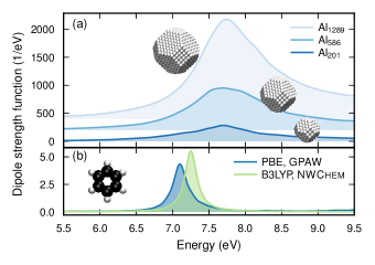
Figure 1: Optical spectra for isolated (a) Al NPs and (b) benzene molecules. All NP data in (a) were obtained from gpaw (RT-TDDFT) using the PBE XC functional. The benzene data in (b) were obtained from gpaw (RT-TDDFT) and NWChem (Casida) calculations using different XC functionals as indicated in the legend.

In the following we consider Al NPs with 201, 586 and 1289 atoms, which exhibit a plasmon resonance at about 7.7 eV (Fig. 1a). Below we analyze their coupling to two or more benzene molecules. The response of the latter is obtained either at the PBE or the B3LYP level yielding the first bright excitation at 7.1 eV and 7.3 eV, respectively (Fig. 1b).

III.2 Coupling as a function of distance

Using the dynamic polarizabilities of the isolated units in Eq. (12), we first inspect the optical spectrum of a system comprising an Al201 NP and two benzene molecules as a function of the NP-molecule distance. Reference data from RT-TDDFT calculations obtained using the PBE XC functional for the full system are available from Refs. 27, 42. These full TDDFT calculations take into account not only coupling to all orders but also charge transfer and renormalization of the underlying states and excitations due to NP-molecule interactions.

The spectra obtained in the DC approximation and from full TDDFT calculations are in good agreement over the entire range of distances considered here (Fig. 2a). Since the DC calculations only include dipolar interactions, the good agreement suggests that for the system under study, higher-order terms, charge transfer, and orbital hybridization play a rather small role in the part of the configuration space considered here.

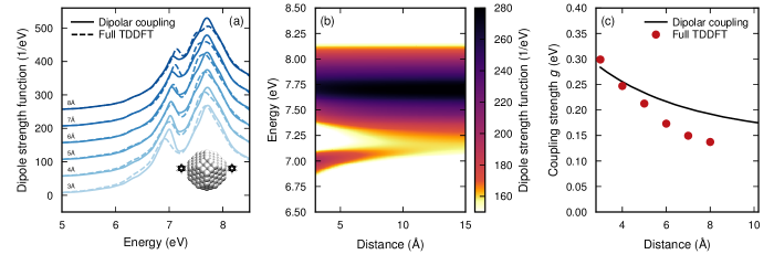
Figure 2: Distance dependence of the optical response from dipolar coupling and full TDDFT calculations. (a) Optical spectra for a system comprising a Al201 NP and two benzene molecules as the NP-molecule distance is varied from RT-TDDFT calculations for the full system (Full TDDFT) and from Eq. (12) (Dipolar coupling). (b) Spectrum of Al201+2 benzene system as a practically continuous function of the NP-molecule distance obtained using the dipolar coupling approximation. (c) Coupling strength extracted from Bayesian fits of the spectra in (a) and (b) to a coupled oscillator model. The extracted values are shown as round markers for the full system (Full TDDFT) and as a solid line for the dipolar coupling calculations.

For the shortest distance of 3 Å a slight underestimation becomes apparent of both position and width of the lower polariton, which we attribute to the absence of orbital overlap and to a lesser extent the neglect of higher-order multipole interactions. In the full TDDFT calculation, the former contribution, which is the more dominant one owing to the fact that higher order multipoles should be even more blue detuned from the benzene transition than the dipolar one, results in a broadening of the benzene transition, which couples with rate $g$ to the Al NP plasmon. An increase of the decay rate ($\gamma$) of one of the strongly coupled elements causes the Rabi splitting $\Omega$ to increase as $\Omega=\sqrt{4g^{2}-(\gamma_{\mathrm{pl}}-\gamma_{\mathrm{ex}})^{2}}$ (for zero detuning) [3], causing the TDDFT-computed polaritons to be broader and farther apart than in the calculations using the DC approximation. Also, since the Al-NP plasmon is blue-detuned from the benzene transition, the two subsystems do not contribute equally to both polaritons. The lower polariton has a more benzene-like character and is more influenced by the width of the benzene transition. Conversely, the upper polariton is more Al-plasmon-like and is not influenced significantly by the decay rate of the molecular transition.

In spite of the limitations discussed in the previous paragraph, the clear strength and benefit of the DC calculations lies in their very rapid computation. Indeed, once the response functions of the individual units have been computed, it is straightforward (and orders of magnitude faster than with full TDDFT modeling) to map out the configuration space. The DC calculations of hybrid systems can even have certain advantages compared to full TDDFT calculations using incomplete basis sets, as numerical factors that can affect the accuracy of the latter are effectively avoided.

Following the evolution of the spectrum as a practically continuous function of the NP-molecule distance reveals the emergence of a clear lower polariton state starting at distances of about 10 Å (Fig. 2b). The coupling strengths $g$ extracted from the DC calculations agree well with the full TDDFT calculations, both with respect to magnitude and distance dependence (Fig. 2c). Interestingly one observes the difference in $g$ between the two types of calculations to increase with distance, which might appear unintuitive at first. This increasing difference stems from the different sources of error in the TDDFT and DC calculations. In the former, the use of localized basis sets that shift in space between calculations induces numerical errors, which exaggerate the blue-shift of the lower polariton at large distances (Supplementary Fig. LABEL:sfig:params). In the latter, the missing effect of state hybridization leads to overly pronounced features, i.e. the polariton peaks are higher and the valley between them deeper. In the coupled oscillator model, an increased value $g$ both makes the lower polariton peak more pronounced and the separation between lower and upper polariton larger.

III.3 Coupling as a function of the number of molecules and NP size

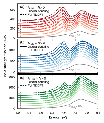
Figure 3: Dependence of the optical response on the number of molecules from dipolar coupling and full TDDFT calculations. Optical spectra of a system comprising (a) a Al201 NP, (b) a Al586 or (c) a Al1289 and a variable number of benzene molecules from RT-TDDFT calculations for the full system (Full TDDFT) and from Eq. (12) (Dipolar coupling). The solid gray lines show the spectrum of the isolated NPs for comparison.

Having confirmed the ability of the DC approximation to reproduce the distance dependence for an Al NP with two benzene molecules and the concomitant emergence of strong coupling, it is now instructive to analyze the spectrum as a function of the number $N$ of benzene molecules, which provides another means for tuning the coupling. As their number increases the effective mass of benzene excitations in the NP-molecule hybrid system increases, enhancing the coupling rate proportionally to the square root of $N$. The resulting large coupling strengths induce much larger changes of the polariton spectra than when the NP-molecule distance is varied. In particular, one notes that both the lower and upper polaritons exhibit significant changes with the Rabi splitting growing monotonically with $N$ [27].

We consider Al NPs with three sizes containing 201, 586 and 1289 atoms coupled to up to eight benzene molecules. Again the DC approximation works well overall, although the agreement becomes worse as NP size and/or the number of benzene molecules increases (Fig. 3).

For the Al201 case with several benzene molecules, one observes a gradual shift of spectral weight from the upper to the lower polariton. For small $N$ it is sensible to attribute the lower (upper) polariton primarily benzene (Al-NP) character. For larger $N$, however, the distinction between plasmonic (Al-NP) and excitonic character (benzene molecule) becomes invalid as the system forms a fully-mixed state (Fig. 3a). This marked change between the balance of the upper and lower polaritons with $N$ is the result of a gradual shift from a red-detuned molecular transition of one benzene with respect to the NP-plasmon to a blue-detuned one for $N=8$ [27]. This change is mostly ascribed to the red-shift of the NP-plasmon with increasing $N$, which may not be captured quantitatively in the DC-approximation. The position of the lower polariton in this Al201 sequence is slightly blue-shifted relative to the full TDDFT data. On the other hand, the DC calculations yield rather sensible results for the width of both polaritons.

By comparison, for the larger Al586 and Al1289 NPs one observes a systematic underestimation of both position and width of the lower polariton (Fig. 3b,c). As noted above (subsection III.2), the differences between DC and TDDFT calculations at a distance of 3 Å are likely related to the absence of orbital hybridization in the DC approximation. The orbital hybridization in TDDFT may also be the cause of other, potentially small, effects that escape the DC approximation. In addition to the above mentioned red-shift of the NP-plasmon, the presence of the molecule may itself modify the mode volume of the cavity (beyond the explicitly studied plasmon-transition coupling) and increase the coupling strength [52].

III.4 Response functions from multiple sources

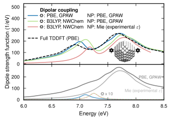
Figure 4: Mixing response calculations from different sources. Optical response of a system comprising Al201 and two benzene molecules at a distance of 3 Å, where the dynamic polarizability of the former is alternatively either by using the PBE XC functional and RT-TDDFT within the gpaw code or by using the Mie approximation in the quasi-static limit with an experimental dielectric function. The dynamic polarizability of the latter is alternatively obtained by using the PBE XC functional and RT-TDDFT within the gpaw code or by using the B3LYP XC functional and Casida LR-TDDFT within the NWChem code. The response of the isolated systems is shown for reference at the bottom of the figure using shaded lines.

While the full TDDFT calculations can capture a variety of contributions that are missed by DC calculations, they are effectively limited by the need to describe the system using one common XC functional. Yet, functionals that perform well for metals are often poorly suited for molecular systems and vice versa. A distinct advantage of the DC approximation is its ability to combine response functions from multiple different sources, including but not limited to different types of electronic structure calculations as well as classical electrodynamics simulations. Here, we specifically exploit this feature to analyze the effect of the XC functional with regard to the description of the excitation spectrum of benzene. Simultaneously, we highlight the possibility for inter-code coupling when using the DC approximation.

We consider a system comprised of a Al201 NP and two benzene molecules at a distance of 3 Å using dynamic polarizabilities calculated using different XC functionals (PBE and B3LYP) and different electronic structure codes (gpaw and NWChem) (Fig. 4). In comparison to PBE, the B3LYP XC functional gives the first bright excitation higher in energy, closer to both the experimental value and the plasmon resonance of the Al NP. The larger spectral overlap leads to less detuning, which primarily manifests itself in a more pronounced transfer of oscillator strength from the upper to the lower polariton. As proof-of-concept, we also demonstrate the DC approximation using the polarizability of a Mie sphere with the dielectric function of bulk Al by McPeak et al. [53] By matching the diameter of the Mie sphere to the distance between opposing {100} facets of the Al201 NP, 16.2 Å, the spectra are similar. We note that the deviation between the Mie spectra based on the dielectric functions measured experimentally by McPeak et al. and Rakic [54] is considerably larger than the deviation between the present calculation and the spectrum based on the data from McPeak et al.

IV Conclusions and outlook

In this study we have analyzed the efficacy of the DC approximation for capturing the emergence of SC in Al NP-benzene hybrid systems. To this end, we compared optical spectra obtained from DC calculations with the results from an earlier study that applied TDDFT to the entire system [27]. We find that overall the DC approximation is able to reproduce the full TDDFT results for this system well over a large size range of considered NPs. Deviations become more pronounced at short NP-molecule distances as orbital overlap and higher-order multipole interactions start to play a role.

After computation of the dynamic polarizabilities of the isolated components, the DC approximation is many orders of magnitude faster than a full scale TDDFT. This enables not only rapid screening of configuration space but computations for much larger systems than those accessible by fully-fledged TDDFT calculations on complete systems (or other first-principles approaches), while still maintaining the underlying accuracy of the individual coupled elements. It thereby becomes possible to study, e.g., ensembles of multiple NPs, mixtures of multiple NPs interacting with multiple molecules or aggregates, and – by extension of the formalism – also the properties of such systems inside of cavities.

The approach employed here has a long history primarily in the context of molecular aggregates [39, 40]. Here, we have demonstrated that it is equally applicable to NP and NP-molecule assemblies. More importantly it is shown that by using dynamic polarizabilities from first-principles calculations near-quantitative predictions become possible also for strongly coupled systems.

We note that calculations via the DC approximation are complementary to electrodynamics simulations using either the finite-difference time-domain method or the discrete dipole approximation, where the latter bears some technical similarities to the present approach. Specifically, DC calculations enable one to address systems with units in the nanometer size range that are commonly difficult or impossible to access using classical electrodynamics.

As noted the DC approximation as used here has shortcomings that need to be addressed in the future. In particular it will break at short NP-NP or NP-molecule distances, where higher-order multipoles and charge transfer effects become important. One should note, however, that particles in solution are usually protected by a ligand shell, which prevents very short particle-particle distances. In the future the approach could therefore be extended to include higher-order multipoles and to account for ligand shells around particles. Since systems of interest often are composed of particles in solution, the dielectric screening due to the solvation medium could also be included in the approach, which can be accomplished via polarizable continuous medium [55] approaches commonly used in quantum chemistry methods. As a final note, it is also of interest to include retardation effects, to accurately describe large systems, and to allow for periodic systems.

Supplementary Material

See supplementary material for details on the fitting of the spectra to the coupled oscillator model.

Data Availability

This study used the TDDFT data published in Ref. 42. The new data generated in this study are openly available via Zenodo at http://doi.org/10.5281/zenodo.4095510, Ref. 56.

Software used

The gpaw package [57, 44] with LCAO basis sets [58] and the LCAO-RT-TDDFT implementation [34] was used for the RT-TDDFT calculations. The NWChem suite [46] was used for Casida LR-TDDFT calculations. The ase library [59] was used for constructing and manipulating atomic structures. The NumPy [60], SciPy [61] and Matplotlib [62] Python packages and the VMD software [63, 64] were used for processing and plotting data. The emcee [65] Python package was used to fit spectra to the coupled oscillator model.

References

- Ebbesen [2016] T. W. Ebbesen, Acc. Chem. Res. 49, 2403 (2016).
- Törmä and Barnes [2015] P. Törmä and W. L. Barnes, Rep. Prog. Phys. 78, 013901 (2015).
- Baranov et al. [2018] D. G. Baranov, M. Wersäll, J. Cuadra, T. J. Antosiewicz, and T. Shegai, ACS Photonics 5, 24 (2018).
- Frisk Kockum et al. [2019] A. Frisk Kockum, A. Miranowicz, S. De Liberato, S. Savasta, and F. Nori, Nat. Rev. Phys. 1, 19 (2019).
- Yoshie et al. [2004] T. Yoshie, A. Scherer, J. Hendrickson, G. Khitrova, H. M. Gibbs, G. Rupper, C. Ell, O. B. Shchekin, and D. G. Deppe, Nature 432, 200 (2004).
- Birnbaum et al. [2005] K. M. Birnbaum, A. Boca, R. Miller, A. D. Boozer, T. E. Northup, and H. J. Kimble, Nature 436, 87 (2005).
- Kasprzak et al. [2006] J. Kasprzak, M. Richard, S. Kundermann, A. Baas, P. Jeambrun, J. M. J. Keeling, F. M. Marchetti, M. H. Szymanska, R. Andre, J. L. Staehli, V. Savona, P. B. Littlewood, B. Deveaud, and L. S. Dang, Nature 443, 409 (2006).
- Hutchison et al. [2012] J. A. Hutchison, T. Schwartz, C. Genet, E. Devaux, and T. W. Ebbesen, Angew. Chem. Int. Ed. 51, 1592 (2012).
- Herrera and Spano [2016] F. Herrera and F. C. Spano, Phys. Rev. Lett. 116, 238301 (2016).
- Galego, Garcia-Vidal, and Feist [2016] J. Galego, F. J. Garcia-Vidal, and J. Feist, Nat. Commun. 7, 13841 (2016).
- Martínez-Martínez et al. [2018] L. A. Martínez-Martínez, R. F. Ribeiro, J. Campos-González-Angulo, and J. Yuen-Zhou, ACS Photonics 5, 167 (2018).
- Munkhbat et al. [2018] B. Munkhbat, M. Wersäll, D. G. Baranov, T. J. Antosiewicz, and T. Shegai, Sci. Adv. 4, eaas9552 (2018).
- Flick and Narang [2020] J. Flick and P. Narang, J. Chem. Phys. 153, 094116 (2020).
- Fregoni et al. [2020] J. Fregoni, G. Granucci, M. Persico, and S. Corni, Chem 6, 250 (2020).
- Thomas et al. [2016] A. Thomas, J. George, A. Shalabney, M. Dryzhakov, S. J. Varma, J. Moran, T. Chervy, X. Zhong, E. Devaux, C. Genet, J. A. Hutchison, and T. W. Ebbesen, Angew. Chem. Int. Ed. 55, 11462 (2016).
- Thomas et al. [2019] A. Thomas, L. Lethuillier-Karl, K. Nagarajan, R. M. A. Vergauwe, J. George, T. Chervy, A. Shalabney, E. Devaux, C. Genet, J. Moran, and T. W. Ebbesen, Science 363, 615 (2019).
- Hirai et al. [2020] K. Hirai, R. Takeda, J. A. Hutchison, and H. Uji-i, Angew. Chem. Int. Ed. 59, 5332 (2020).
- Feist and Garcia-Vidal [2015] J. Feist and F. J. Garcia-Vidal, Phys. Rev. Lett. 114, 196402 (2015).
- Zhong et al. [2016] X. Zhong, T. Chervy, S. Wang, J. George, A. Thomas, J. A. Hutchison, E. Devaux, C. Genet, and T. W. Ebbesen, Angew. Chem. Int. Ed. 55, 6202 (2016).
- Jaynes and Cummings [1963] E. T. Jaynes and F. W. Cummings, Proc. IEEE 51, 89 (1963).
- Garraway [2011] B. M. Garraway, Phil. Trans. R. Soc. A 369, 1137 (2011).
- Galego, Garcia-Vidal, and Feist [2015] J. Galego, F. J. Garcia-Vidal, and J. Feist, Phys. Rev. X 5, 041022 (2015).
- Ruggenthaler et al. [2014] M. Ruggenthaler, J. Flick, C. Pellegrini, H. Appel, I. V. Tokatly, and A. Rubio, Phys. Rev. A 90, 012508 (2014).
- Flick et al. [2017] J. Flick, M. Ruggenthaler, H. Appel, and A. Rubio, Proc. Natl. Acad. Sci. U.S.A. 114, 3026 (2017).
- Ling Luk et al. [2017] H. Ling Luk, J. Feist, J. J. Toppari, and G. Groenhof, J. Chem. Theory Comput. 13, 4324 (2017).
- Neuman et al. [2018] T. Neuman, R. Esteban, D. Casanova, F. J. Garcia-Vidal, and J. Aizpurua, Nano Lett. 18, 2358 (2018).
- Rossi et al. [2019a] T. P. Rossi, T. Shegai, P. Erhart, and T. J. Antosiewicz, Nat. Commun. 10, 3336 (2019a).
- Flick et al. [2019] J. Flick, D. M. Welakuh, M. Ruggenthaler, H. Appel, and A. Rubio, ACS Photonics 6, 2757 (2019).
- Orgiu et al. [2015] E. Orgiu, J. George, J. Hutchison, E. Devaux, J. Dayen, B. Doudin, F. Stellacci, C. Genet, J. Schachenmayer, C. Genes, G. Pupillo, P. Samori, and T. Ebbesen, Nat. Mater. 14, 1123 (2015).
- Hohenberg and Kohn [1964] P. Hohenberg and W. Kohn, Phys. Rev. 136, B864 (1964).
- Kohn and Sham [1965] W. Kohn and L. Sham, Phys. Rev. 140, A1133 (1965).
- Runge and Gross [1984] E. Runge and E. Gross, Phys. Rev. Lett. 52, 997 (1984).
- Yabana and Bertsch [1996] K. Yabana and G. F. Bertsch, Phys. Rev. B 54, 4484 (1996).
- Kuisma et al. [2015] M. Kuisma, A. Sakko, T. Rossi, A. Larsen, J. Enkovaara, L. Lehtovaara, and T. Rantala, Phys. Rev. B 91, 115431 (2015).
- Casida [1995] M. E. Casida, in Recent Advances in Density Functional Methods, Part I, edited by D. P. Chong (World Scientific, Singapore, 1995) p. 155.
- Casida [2009] M. E. Casida, J. Mol. Struct. THEOCHEM 914, 3 (2009).
- Mie [1908] G. Mie, Ann. Phys. 25, 377 (1908).
- Sihvola [2007] A. Sihvola, J. Nanomat. 2007, 1 (2007).
- DeVoe [1964] H. DeVoe, J. Chem. Phys. 41, 393 (1964).
- Fidder, Knoester, and Wiersma [1991] H. Fidder, J. Knoester, and D. A. Wiersma, J. Chem. Phys. 95, 7880 (1991).
- Auguié, Darby, and Ru [2019] B. Auguié, B. L. Darby, and E. C. L. Ru, Nanoscale 11, 12177 (2019).
- Rossi et al. [2019b] T. P. Rossi, T. Shegai, P. Erhart, and T. J. Antosiewicz, Zenodo (2019b), 10.5281/zenodo.3242317.
- Perdew, Burke, and Ernzerhof [1996] J. P. Perdew, K. Burke, and M. Ernzerhof, Phys. Rev. Lett. 77, 3865 (1996).
- Enkovaara et al. [2010] J. Enkovaara, C. Rostgaard, J. J. Mortensen, J. Chen, M. Dułak, L. Ferrighi, J. Gavnholt, C. Glinsvad, V. Haikola, H. A. Hansen, H. H. Kristoffersen, M. Kuisma, A. H. Larsen, L. Lehtovaara, M. Ljungberg, O. Lopez-Acevedo, P. G. Moses, J. Ojanen, T. Olsen, V. Petzold, N. A. Romero, J. Stausholm-Møller, M. Strange, G. A. Tritsaris, M. Vanin, M. Walter, B. Hammer, H. Häkkinen, G. K. H. Madsen, R. M. Nieminen, J. K. Nørskov, M. Puska, T. T. Rantala, J. Schiøtz, K. S. Thygesen, and K. W. Jacobsen, J. Phys.: Condens. Matter 22, 253202 (2010).
- Blöchl [1994] P. E. Blöchl, Phys. Rev. B 50, 17953 (1994).
- Valiev et al. [2010] M. Valiev, E. J. Bylaska, N. Govind, K. Kowalski, T. P. Straatsma, H. J. J. Van Dam, D. Wang, J. Nieplocha, E. APhysical Review A, T. L. Windus, and W. A. de Jong, Comput. Phys. Commun. 181, 1477 (2010).
- Lee, Yang, and Parr [1988] C. Lee, W. Yang, and R. G. Parr, Phys. Rev. B 37, 785 (1988).
- Becke [1993] A. D. Becke, J. Chem. Phys. 98, 5648 (1993).
- McLean and Chandler [1980] A. D. McLean and G. S. Chandler, J. Chem. Phys. 72, 5639 (1980).
- Krishnan et al. [1980] R. Krishnan, J. S. Binkley, R. Seeger, and J. A. Pople, J. Chem. Phys. 72, 650 (1980).
- Wu, Gray, and Pelton [2010] X. Wu, S. K. Gray, and M. Pelton, Opt. Express 18, 23633 (2010).
- Yang, Antosiewicz, and Shegai [2016] Z.-J. Yang, T. J. Antosiewicz, and T. Shegai, Opt. Express 24, 20373 (2016).
- McPeak et al. [2015] K. M. McPeak, S. V. Jayanti, S. J. P. Kress, S. Meyer, S. Iotti, A. Rossinelli, and D. J. Norris, ACS Photonics 2, 326 (2015).
- Rakić [1995] A. D. Rakić, Appl. Opt. 34, 4755 (1995).
- Barone, Cossi, and Tomasi [1997] V. Barone, M. Cossi, and J. Tomasi, J. Chem. Phys. 107, 3210 (1997).
- Fojt et al. [2021] J. Fojt, T. P. Rossi, T. J. Antosiewicz, M. Kuisma, and P. Erhart, Zenodo (2021), 10.5281/zenodo.4095510.
- Mortensen, Hansen, and Jacobsen [2005] J. Mortensen, L. Hansen, and K. Jacobsen, Phys. Rev. B 71, 035109 (2005).
- Larsen et al. [2009] A. Larsen, M. Vanin, J. Mortensen, K. Thygesen, and K. Jacobsen, Phys. Rev. B 80, 195112 (2009).
- Larsen et al. [2017] A. Larsen, J. Mortensen, J. Blomqvist, I. Castelli, R. Christensen, M. Dulak, J. Friis, M. Groves, B. Hammer, C. Hargus, E. Hermes, P. Jennings, P. Jensen, J. Kermode, J. Kitchin, E. Kolsbjerg, J. Kubal, K. Kaasbjerg, S. Lysgaard, J. Maronsson, T. Maxson, T. Olsen, L. Pastewka, A. Peterson, C. Rostgaard, J. S. O. Schütt, M. Strange, K. Thygesen, T. Vegge, L. Vilhelmsen, M. Walter, Z. Zeng, and K. W. Jacobsen, J. Phys.: Condens. Matter 29, 273002 (2017).
- Harris et al. [2020] C. R. Harris, K. J. Millman, S. J. van der Walt, R. Gommers, P. Virtanen, D. Cournapeau, E. Wieser, J. Taylor, S. Berg, N. J. Smith, R. Kern, M. Picus, S. Hoyer, M. H. van Kerkwijk, M. Brett, A. Haldane, J. F. del Río, M. Wiebe, P. Peterson, P. Gérard-Marchant, K. Sheppard, T. Reddy, W. Weckesser, H. Abbasi, C. Gohlke, and T. E. Oliphant, Nature 585, 357 (2020).
- Virtanen et al. [2020] P. Virtanen, R. Gommers, T. E. Oliphant, M. Haberland, T. Reddy, D. Cournapeau, E. Burovski, P. Peterson, W. Weckesser, J. Bright, S. J. van der Walt, M. Brett, J. Wilson, K. J. Millman, N. Mayorov, A. R. J. Nelson, E. Jones, R. Kern, E. Larson, C. J. Carey, İ. Polat, Y. Feng, E. W. Moore, J. VanderPlas, D. Laxalde, J. Perktold, R. Cimrman, I. Henriksen, E. A. Quintero, C. R. Harris, A. M. Archibald, A. H. Ribeiro, F. Pedregosa, P. van Mulbregt, and SciPy 1.0 Contributors, Nat. Methods 17, 261 (2020).
- Hunter [2007] J. D. Hunter, Comput. Sci. Eng. 9, 90 (2007).
- Humphrey, Dalke, and Schulten [1996] W. Humphrey, A. Dalke, and K. Schulten, J. Mol. Graph. 14, 33 (1996).
- Stone [1998] J. Stone, An Efficient Library for Parallel Ray Tracing and Animation, Master’s thesis, Computer Science Department, University of Missouri-Rolla (1998).
- Foreman-Mackey et al. [2013] D. Foreman-Mackey, D. W. Hogg, D. Lang, and J. Goodman, Publ. Astron. Soc. Pac. 125, 306 (2013).