Neuro-Reachability of Networked Microgrids

Abstract

A neural ordinary differential equations network (ODE-Net)-enabled reachability method (Neuro-Reachability) is devised for the dynamic verification of networked microgrids (NMs) with unidentified subsystems and heterogeneous uncertainties. Three new contributions are presented: 1) An ODE-Net-enabled dynamic model discovery approach is devised to construct the data-driven state-space model which preserves the nonlinear and differential structure of the NMs system; 2) A physics-data-integrated (PDI) NMs model is established, which empowers various NM analytics; and 3) A conformance-empowered reachability analysis is developed to enhance the reliability of the PDI-driven dynamic verification. Extensive case studies demonstrate the efficacy of the ODE-Net-enabled method in microgrid dynamic model discovery, and the effectiveness of the Neuro-Reachability approach in verifying the NMs dynamics under multiple uncertainties and various operational scenarios.

I Introduction

Networked microgrids (NMs) allow microgrids to support coordinately various smart community functions [1] and help increase electricity resilience [2, 3]. However, two major challenges arise in the dynamic analysis of today’s low-inertia NMs [4], which prevent NMs from serving as dependable resiliency resources: I) Lack of effective analytics to handle the combinatorial explosion in verifying the NMs dynamics under the infinitely many uncertain scenarios [5], and II) Unattainablility of accurate models for each and every microgrid, especially the dynamic models of converters, loads and circuits [6, 7].

Reachability analysis is a novel method which can provably enclose all dynamic trajectories under uncertain perturbations and large disturbances in NMs [5, 8, 9]. It prevails over traditional time-domain simulations [10] and energy function approaches [11, 12] mainly due to the capability of processing infinitely many uncertain scenarios efficiently. Even though reachability analysis is proved to be a promising solution to Challenge I, Challenge II above has been a major obstacle that prevents it from being widely adopted in the planning and operations of NMs.

Learning reliable dynamic models for the unidentified subsystems from measurements, therefore, is of paramount importance for the data-driven NMs dynamic analysis. Koopman operator and dynamic mode decomposition are popular approaches to constructing linear approximation of nonlinear systems from data [13, 14], whereas they are inefficient to establish nonlinear ODE models for rapidly-fluctuating NMs subject to ‘random walks’ of operating points disturbed by uncertainties [15]. Plenty of machine learning approaches have been applied for power system dynamic analysis, either for the time-domain trajectory prediction [16] or for the stability classification [17, 18]. Nevertheless, discovering dynamic models behind data, which is a long standing open problem, is substantially more important in the sense of providing deep insights of the system dynamics and allowing for formal verifications and control of the system.

The overarching goal of this paper is to establish a data-driven method well suited to discovering the strongly nonlinear NMs dynamics as well as to verifying the NMs dynamics under uncertainties. To this end, this paper devises a Neuro-Reachability method. The key innovation is to integrate the neural ordinary differential equations network (ODE-Net) with reachability analysis and conformance theory to allow for a data-driven formal verification of the NMs dynamics under uncertainties. The contributions of this work are threefold:

• An ODE-Net-enabled model discovery method is devised to construct a nonlinear ODE model for the uncertainty-perturbed NMs, which can best preserve the dynamic behaviours of NMs without assuming a priori any specific dynamic modes. This modeling approach can effectively address the data rich, information poor (DRIP) problem widely existing in today’s microgrids.

• A physics-data-integrated (PDI) modelling approach is then introduced to combine both physics-based and data-driven ODE models, which enables reachability analysis to verify the PDI-NMs dynamics incorporating the hierarchical control of DERs and network transients.

• Reachability analysis for NMs is further empowered with a conformance theory as a ‘feedback’ mechanism to further improve the reachset accuracy induced by possible inconformance of the PDI-NMs behaviours compared with the real NMs dynamics.

The remainder of the paper is organized as follows. Section II introduces the ODE-Net-enabled dynamic model discovery. Section III establishes the NMs model integrated by both physics-based and data-driven subsystems. Section IV devises the conformance-empowered reachability analysis for the PDI-NMs dynamics. Section V presents case studies on a typical NMs system to validate the Neuro-Reachability method. Finally, Section VI concludes the paper.

II ODE-Net-Enabled Dynamic Model Discovery for Microgrids

Pursuant to the attainablility of physics models, the overall NMs system can always be partitioned into an internal subsystem (InSys) and an external subsystem (ExSys), as illustrated in Fig. 1. InSys, where the structure and parameters are precisely known, can be readily formulated by assembling the dynamic models of its components. ExSys, in contrast, has to be modeled via a data-driven approach due to the absence of physics models, the unavailability of state measurements, and/or the need to preserve the consumer privacy.

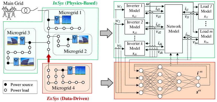
Figure 1: Illustration of NMs modeling with physics-based InSys and data-driven ExSys

This section devises an ODE-Net-enabled method to discover a state-space model of ExSys.

II-A ODE-Net-Based State-Space Model Formulation

The functional formulation of ExSys is established as

$$\dot{\bm{x}}=\mathcal{N}(\bm{x},\bm{u})$$ (1)

Here, function $\mathcal{N}$ represents a state-space form of ExSys and is to be learned from the measurements; $\bm{x}$ and $\bm{u}$ respectively denote the state variables and input variables of ExSys. This ODE-governed, learned ExSys model can be integrated with the InSys model for assessing the overall NMs dynamics. Details of $\bm{x}$ and $\bm{u}$ are introduced in Subsection III-B.

Fig. 2 illustrates the dynamic model discovery using ODE-Net. Taking $\bm{x}$ and $\bm{u}$ at time $t$ as the inputs, ODE-Net outputs the time derivative of $\bm{x}$ and therefore explicitly establishes the ExSys dynamic model in (1) by the forward propagation in the neural network.

Given a time series of NMs trajectories as $\{(t_{1},t_{2},\dots,t_{n}),(\hat{\bm{x}}_{1},\hat{\bm{x}}_{2},\dots,\hat{\bm{x}}_{n}),(\hat{\bm{u}}_{1},\hat{\bm{u}}_{2},\dots,\hat{\bm{u}}_{n})\}$, ODE-Net best matches the ExSys dynamics by minimizing the error between the state measurements $\hat{\bm{x}}$ and the numerical solution of (1):

$$\min_{\bm{\theta}}\sum_{i=1}^{n}L(\bm{x}_{i})=\sum_{i=1}^{n}\frac{1}{2}\eta_{i}\|\bm{x}_{i}-\hat{\bm{x}}_{i}\|_{2}$$ (2)

$$s.t.~{}~{}\bm{x}_{i}=\hat{\bm{x}}_{1}+\int_{t_{1}}^{t_{i}}\mathcal{N}(\bm{x},\bm{u},\bm{\theta})\differential t$$

where $\bm{\theta}$ denotes the ODE-Net parameters; $\eta_{i}$ denotes the weighting factor at time point $i$.

Figure 2: ODE-Net-enabled dynamic model discovery of ExSys

II-B Continuous Backpropagation Technique

The main difficulty in the optimization of (2) lies in the ODE integration operation in the constraints. In this subsection, the continuous propagation technique [19] is applied to handle the ODE integration in the ODE-Net training.

Lagrange multiplier $\bm{\lambda}$ is first introduced to (2) to remove the ODE constraints and build the following loss function:

$$\mathcal{L}=\sum_{i=1}^{n}L(\bm{x}_{i})-\int_{t_{0}}^{t_{n}}\bm{\lambda}^{T}\left(\dot{\bm{x}}-\mathcal{N}(\bm{x},\bm{u},\bm{\theta})\right)\differential t$$ (3)

Backpropagation computes the gradient of the loss function with respect to the ODE-Net parameters to minimize the loss function  [20]. With the loss function (3) involving the integration operator, the partial derivative of $\mathcal{L}$ with respect to $\bm{\theta}$ is calculated as:

$$\partialderivative{\mathcal{L}}{\bm{\theta}}= \sum_{i=1}^{n}\left(\partialderivative{L}{\bm{x}_{i}}\partialderivative{\bm{x}_{i}}{\bm{\theta}}-\int_{t_{i-1}}^{t_{i}}\bm{\lambda}^{T}\left(\partialderivative{\dot{\bm{x}}}{\bm{\theta}}-\partialderivative{\mathcal{N}}{\bm{x}}\partialderivative{\bm{x}}{\bm{\theta}}-\partialderivative{\mathcal{N}}{\bm{\theta}}\right)\differential t\right)$$

$$= \sum_{i=1}^{n}\partialderivative{L}{\bm{x}_{i}}\partialderivative{\bm{x}_{i}}{\bm{\theta}}+\sum_{i=1}^{n}\left(\bm{\lambda}^{T}(t_{i}^{-})\partialderivative{\bm{x}_{i}}{\bm{\theta}}-\bm{\lambda}^{T}(t_{i-1}^{+})\partialderivative{\bm{x}_{i-1}}{\bm{\theta}}\right)$$

$$+\sum_{i=1}^{n}\int_{t_{i-1}}^{t_{i}}\left(\derivative{\bm{\lambda}^{T}}{t}\partialderivative{\bm{x}}{\bm{\theta}}+\bm{\lambda}^{T}\partialderivative{\mathcal{N}}{\bm{x}}\partialderivative{\bm{x}}{\bm{\theta}}+\bm{\lambda}^{T}\partialderivative{\mathcal{N}}{\bm{\theta}}\right)\differential t$$

   (4)

The Lagrange multiplier variables are given by [21]:

$$\derivative{\bm{\lambda}^{T}}{t}=-\bm{\lambda}^{T}\partialderivative{\mathcal{N}}{\bm{x}}$$ (5)

where the boundary conditions are set as:

$$\bm{\lambda}^{T}(t_{n}^{+})=0~{}~{},~{}~{}\bm{\lambda}^{T}(t_{i}^{+})=\bm{\lambda}^{T}(t_{i}^{-})+\partialderivative*{L}{\bm{x}_{i}}$$ (6)

Then, (4) can be derived into:

$$\partialderivative{\mathcal{L}}{\bm{\theta}}=\int_{t_{0}}^{t_{n}}\bm{\lambda}^{T}\partialderivative{\mathcal{N}}{\bm{\theta}}\differential t$$ (7)

Collecting (5) and (7) leads to an ODE integration problem:

$$\derivative{t}\begin{bmatrix}\bm{\lambda}^{T}\\ \partialderivative*{\mathcal{L}}{\bm{\theta}}\end{bmatrix}=\begin{bmatrix}-\bm{\lambda}^{T}\partialderivative*{\mathcal{N}}{\bm{x}}\\ \bm{\lambda}^{T}\partialderivative*{\mathcal{N}}{\bm{\theta}}\end{bmatrix}$$ (8)

Subsequently, $\partialderivative*{\mathcal{L}}{\bm{\theta}}$ can be obtained from (8) by any ODE solver, e.g., Trapezoidal integration. Given the final value of $\lambda(t)$, i.e., $\bm{\lambda}^{T}(t_{n})$ in (6), rather than the initial value, (8) requires solving the ODEs backwards in time, which leads to a reverse-mode integration [19]:

$$\evaluated{\partialderivative{\mathcal{L}}{\bm{\theta}}}_{t_{1}}=\evaluated{\partialderivative{\mathcal{L}}{\bm{\theta}}}_{t_{n}}+\int_{t_{n}}^{t_{1}}\bm{\lambda}^{T}\partialderivative{\mathcal{N}}{\bm{\theta}}\differential t=\sum_{i=2}^{n}\int_{t_{i}}^{t_{i-1}}\bm{\lambda}^{T}\partialderivative{\mathcal{N}}{\bm{\theta}}\differential t$$ (9)

with $\bm{\lambda}(t)$ also solved by the reverse-mode integration:

$$\bm{\lambda}^{T}(t_{i-1}^{+})=\bm{\lambda}^{T}(t_{i}^{-})+\int_{t_{i}}^{t_{i-1}}\bm{\lambda}^{T}\partialderivative{\mathcal{N}}{\bm{x}}\differential t$$ (10)

Further, consider a set of time series of NMs trajectories as $\{(\bm{t}^{(1)},\hat{\bm{x}}^{(1)},\hat{\bm{u}}^{(1)}),\dots,(\bm{t}^{(m)},\hat{\bm{x}}^{(m)},\hat{\bm{u}}^{(m)})\}$. For the $j^{th}$ measurement, let $\partialderivative*{\mathcal{L}^{(j)}}{\bm{\theta}}$ be the gradient of the loss function computed by (9). The overall gradient is obtained:

$$\partialderivative{\mathcal{L}}{\bm{\theta}}=\sum\nolimits_{j=1}^{m}\partialderivative{\mathcal{L}^{(j)}}{\bm{\theta}}$$ (11)

Consequently, the ODE-Net parameters are updated using gradient descent so that $\mathcal{L}$ can be decreased during training:

$$\bm{\theta}\longleftarrow\bm{\theta}-r\partialderivative{\mathcal{L}}{\bm{\theta}}$$ (12)

where $r$ denotes the learning rate.

The continuous backpropagation incorporates the “ODE solver” in the gradient descent for the ODE-Net parameter optimization, and hence effectively retains the intrinsic continuous differential structure of the dynamical NMs.

II-C Continuous Network Structure

Despite the capability of modeling complicated nonlinear dynamics, a deep ODE-Net involves a large number of parameters and prohibitively high cost for computing $\partialderivative*{\mathcal{N}}{\bm{x}}$ and $\partialderivative*{\mathcal{N}}{\bm{\theta}}$ in the continuous backpropagation. To resolve this problem, this paper uses a continuous-depth network, which enables a linear memory cost with network depth and controllable numerical error [19].

In a classical neural network, the hidden layers follow a discrete structure (i.e., layers 1, 2, $\cdots$, $K$ as illustrated by the solid-line neurons in Fig. 2), and therefore formulates a set of difference equations for forward propagation:

$$\bm{z}_{k+1}=\bm{z}_{k}+\bm{h}(\bm{z}_{k},\bm{\theta}_{k})$$ (13)

Here, $k\in\mathbb{N}^{+}$ denotes the discrete layer; $\bm{z}_{k}$ and $\bm{\theta}_{k}$ respectively denote the output states and parameters of the $k^{th}$ hidden layer.

The continuous-depth network regards the forward propagation of the discrete layers in (13) as an Euler discretization of a set of continuous differential equations, i.e., it continuously propagates the states from the input layer to the output layer (see the dotted-line neurons in Fig. 2 ). This idea leads to a continuous “layer dynamics”:

$$\derivative{\bm{z}(k)}{k}=\bm{h}(\bm{z}(k),\bm{\theta}_{h})\Longrightarrow\bm{z}_{K}=\bm{z}_{1}{+}\int_{1}^{K}\bm{h}(\bm{z},\bm{\theta}_{h})\differential k$$ (14)

Here, $k\in\mathbb{R}^{+}$ denotes the continuous layer; $\bm{z}(k)$ and $\bm{\theta}_{h}$ respectively denote the output states and parameters of the continuous hidden layer. As can be seen from (14), $\bm{z}_{K}$, i.e., the final output of the hidden layer, can be directly obtained by integrating over the continuous layers.

Based on the continuous-depth network, the chain rule is applied to compute $\partialderivative*{\mathcal{N}}{\bm{x}}$ and $\partialderivative*{\mathcal{N}}{\bm{x}}$ for (8):

$$\partialderivative{\mathcal{N}}{\bm{x}}=\bm{\theta}_{K}^{T}\partialderivative{\bm{z}_{K}}{\bm{z}_{1}}\partialderivative{\bm{z}_{1}}{\bm{x}}~{}~{},~{}~{}\partialderivative{\mathcal{N}}{\bm{\theta}_{h}}=\bm{\theta}_{K}^{T}\partialderivative{\bm{z}_{K}}{\bm{\theta}_{h}}$$ (15)

To obtain $\partialderivative*{\bm{z}_{K}}{\bm{z}_{1}}$ and $\partialderivative*{\bm{z}_{K}}{\bm{\theta}_{h}}$ in the equation above, the reverse-mode ODE integration discussed in Subsection II-B is again applied. Specifically, in analogy to (3), the following ODEs are formulated [19] for the gradient of $\bm{z}_{K}$ with respect to $\bm{z}(k)$:

$$\derivative{k}\begin{bmatrix}\partialderivative*{\bm{z}_{K}}{\bm{z}}\\ \partialderivative*{\bm{z}_{K}}{\bm{\theta}_{h}}\end{bmatrix}=\begin{bmatrix}-(\partialderivative*{\bm{z}_{K}}{\bm{z}})^{T}\partialderivative*{\bm{h}}{\bm{z}}\\ (\partialderivative*{\bm{z}_{K}}{\bm{z}})^{T}\partialderivative*{\bm{h}}{\bm{\theta}_{h}}\end{bmatrix}$$ (16)

Then, in analogy to (11) and (12), the numerical solution of (16), i.e., $\partialderivative*{\bm{z}_{K}}{\bm{z}_{1}}$ and $\partialderivative*{\bm{z}_{K}}{\bm{\theta}_{h}}$, is obtained by the ODE integration.

III Physics-Data-Integrated ODE Modeling for NMs Dynamics

Based on the ODE-Net-enabled ExSys formulation, this section establishes the overall dynamic model of NMs by combining the physics-based InSys and data-driven ExSys, as illustrated in Fig. 1.

III-A Physics-Based Formulation of InSys

Given the model of each component (e.g., a DER, a power load, a branch), InSys can be explicitly formulated as a system of differential algebraic equations (DAEs):

$$\dot{\bm{s}}^{in}=\bm{g}^{in}(\bm{s}^{in},\bm{i}^{in},\bm{w}^{in},\bm{s}^{ex})$$ (17a)

$$\dot{\bm{i}}^{in}=\bm{f}^{in}(\bm{s}^{in},\bm{i}^{in})+\bm{m}^{in}\bm{v}$$ (17b)

$$\bm{n}^{in}\bm{i}^{in}+\bm{n}^{ex}\bm{i}^{ex}=\bm{0}$$ (17c)

Here, (17a) formulates the dynamics of each component in InSys, where $\bm{s}^{in}$ denotes the state variables of each component; $\bm{i}^{in}$ denotes the current injections from each component and is normally formulated under the DQ coordinates for the inverter-dominated NMs; $\bm{w}^{in}$ denotes the uncertain inputs caused by DERs in InSys; $\bm{s}^{ex}$ includes (but not limited to) the control variables sent from ExSys, which is particularly used to account for the global control effects; function $\bm{g}^{in}$ is formulated according to the dynamics of each component. Equation (17b) formulates the current injections from each component, where $\bm{v}$ denotes the DQ-axis voltages at each bus of InSys and boundary buses of ExSys; $\bm{m}^{in}$ denotes the DQ-axis incidence matrix between components and buses. Equation (17c) formulates the Kirchhoff’s Current Law at the buses of InSys and boundary buses of ExSys, where $\bm{i}^{ex}$ denotes the current injections from ExSys; matrices $\bm{n}^{in}$ and $\bm{n}^{ex}$ denotes the directed component-bus incidence matrix.

III-B Data-Driven Formulation of ExSys

Following (17), ExSys interacts with InSys through its current injections $\bm{i}_{ex}$ and control signals $\bm{s}_{ex}$. Therefore, $\bm{i}_{ex}$ and $\bm{s}_{ex}$ are retained for dynamic simulations of InSys. Accordingly, ExSys is formulated as:

$$\dot{\bm{s}}^{ex}=\bm{g}^{ex}(\bm{i}^{in},\bm{s}^{in},\bm{i}^{ex},\bm{s}^{ex},\bm{w}^{in},\bm{w}^{ex})$$ (18a)

$$\dot{\bm{i}}^{ex}=\bm{f}^{ex}(\bm{i}^{in},\bm{s}^{in},\bm{i}^{ex},\bm{s}^{ex},\bm{w}^{in},\bm{w}^{ex})$$ (18b)

Here, (18a) formulates the dynamics of control variables sending from ExSys to InSys; (18b) formulates the dynamics of the current injections from ExSys; $\bm{w}^{ex}$ denotes the uncertain factors in ExSys.

ODE-Net is used to establish the ODE model in (18), following the procedures in Section II. The ExSys formulation in (1) can now be expanded by: $\mathcal{N}=[\bm{g}^{ex};\bm{f}^{ex}]$ denoting the dynamics of ExSys; $\bm{x}=[\bm{s}^{ex};\bm{i}^{ex}]$ denoting the state variables of ExSys; and $\bm{u}=[\bm{i}^{in};\bm{s}^{in};\bm{w}^{in};\bm{w}^{ex}]$ assembling the input variables in (18).

III-C Physics-Data-Integrated (PDI) NMs Model

The entire NMs model is established by combining the physics-based formulation of InSys and data-driven formulation of ExSys:

$$[left=\empheqlbrace\,] \dot{\bm{s}}=\bm{g}(\bm{i},\bm{s},\bm{w})$$ (19a)

$$\dot{\bm{i}}=\bm{f}(\bm{i},\bm{s},\bm{w})+\bm{mv}$$ (19b)

$$\bm{0}=\bm{ni}$$ (19c)

where $\bm{s}$, $\bm{i}$ and $\bm{w}$ respectively assemble the state variables, current injections and uncertainties of InSys and ExSys.

The DAE model in (19) can be rigorously converted to a system of nonlinear ODEs [22], as briefly introduced below. Denote the matrix constructed by the maximal linearly independent columns of $\bm{n}$ as $\bm{n}_{1}$, and the matrix constructed by the other columns as $\bm{n}_{0}$. Since $\bm{n}_{1}$ is non-singular, (19c) leads to the following:

$$\bm{n}_{0}\bm{i}_{0}+\bm{n}_{1}\bm{i}_{1}=\bm{0}\Longrightarrow\bm{i}_{1}=-\bm{n}_{1}^{-1}\bm{n}_{0}\bm{i}_{0}$$ (20)

where $\bm{i}_{0}$ and $\bm{i}_{1}$ respectively denote the sub-vectors of $\bm{i}$ corresponding to $\bm{n}_{0}$ and $\bm{n}_{1}$.

Taking derivative of (19c) yields the following:

$$\bm{0}=\bm{n}\dot{\bm{i}}=\bm{n}\hat{\bm{f}}(\bm{i}_{0},\bm{s})+\bm{nm}\bm{v}\Longrightarrow\bm{v}=-(\bm{nm})^{-1}\bm{n}\hat{\bm{f}}$$ (21)

where $\hat{\bm{f}}(\bm{i}_{0},\bm{s},\bm{w})=\bm{f}(\bm{i},\bm{s},\bm{w})$ by substituting (20) to $\bm{f}$.

Therefore, (19) is converted to an ODE model:

$$[left=\empheqlbrace\,] \dot{\bm{s}}=\hat{\bm{g}}(\bm{i}_{0},\bm{s},\bm{w})$$ (22a)

$$\dot{\bm{i}}_{0}=-\bm{m}_{0}(\bm{nm})^{-1}\bm{n}\hat{\bm{f}}(\bm{i}_{0},\bm{s})+\hat{\bm{f}}_{0}(\bm{i}_{0},\bm{s})$$ (22b)

where $\bm{m}_{0}$ and $\hat{\bm{f}}_{0}$ respectively extract the components of $\bm{m}$ and $\hat{\bm{f}}$ corresponding to $\bm{i}_{0}$.

The obtained ODE model in (22) is rigorously equivalent to the original DAE model (19a) without adopting any linearization. Hence, it can be used for the transient analysis under small or large disturbances. The PDI-NMs model in (22) can then be abstracted as:

$$\dot{\bm{X}}=\bm{F}(\bm{X},\bm{W})$$ (23)

where $\bm{X}$ denotes the state variables of NMs integrating states of both InSys and ExSys; $\bm{W}$ denotes to the uncertainty inputs.

IV Neuro-Reachability Analysis of NMs Dynamics

Based on the PDI-NMs model, this section devises a Neuro-Reachability method for dynamic verification of NMs.

IV-A Reachset For NMs

Reachability analysis verifies the NMs dynamics by calculating reachsets, i.e., a provable enclosure of all possible dynamic trajectories under infinitely many uncertain scenarios. Given the set of initial NMs states $\mathcal{X}^{0}$ and the set of DER uncertainties $\mathcal{W}$, the time-point reachset is defined as the set of all the possible NMs states at time $t$:

$$\mathcal{R}(t)= \Bigl{\{}\bm{X}(t)=\int_{0}^{t}\bm{F}(\bm{X}(\tau),\bm{W}(\tau))\differential\tau\Bigm{|}$$ (24)

$$~{}~{}\bm{X}(0)\in\mathcal{X}^{0},\bm{W}\in\mathcal{W}\Bigr{\}}$$

In this research, the uncertainty set $\mathcal{W}$ is formulated by an unknown-but-bounded set; and zonotope bundle is utilized for set formulation [23], i.e., an intersection of finite zonotopes which is able to represent arbitrary polytopes with a satisfactory computational efficiency.

Applying Taylor expansion to (23) at $(\bm{X}^{*},\bm{W}^{*})$ gives:

$$\dot{\bm{X}}\in\bm{F}^{*}+\bm{J}(\bm{X}-\bm{X}^{*})+\bm{J}_{w}(\bm{W}-\bm{W}^{*})+\bm{e}_{l}$$ (25)

where $\bm{F}^{*}=\bm{F}(\bm{X}^{*},\bm{W}^{*})$; $\bm{J}=\partialderivative*{\bm{F}^{*}}{\bm{X}}$ and $\bm{J}_{w}=\partialderivative*{\bm{F}^{*}}{\bm{W}}$ respectively denote the Jacobian matrix referring to the first-order Taylor series; $\bm{e}_{l}$ is the Lagrange remainder [24]. For computational convenience, $\mathcal{R}(t)$ is shifted to $\mathcal{R}(t)-\bm{X}^{*}$ to perform the set computation. Therefore, the time-point reachset of the NMs dynamics can be computed by the evolution of the previous time-point reachset:

$$\mathcal{R}(t)=\left(e^{\bm{J}\Delta}\mathcal{R}(t-\Delta)\right)\oplus\int_{0}^{\Delta}e^{\bm{J}(\Delta-\tau)}\mathcal{W}_{F}\differential\tau\oplus\mathcal{R}_{el}$$ (26)

where $\Delta$ denotes the time step; $\oplus$ denotes the Minkowski addition. In (26), the first term computes the reachset propagation resulting from the NMs states, i.e., $\bm{J}(\bm{X}-\bm{X}^{*})$. The second term computes the reachset propagation resulting from the inputs $\mathcal{W}_{F}=\bm{J}_{w}(\mathcal{W}-\bm{W}^{*})+\bm{F}^{*}$, which composes both the uncertainty impact $\bm{J}_{w}(\bm{W}-\bm{W}^{*})$ and the linearization point impact $\bm{F}^{*}$. And the third term in (26) computes the set of linearization error [24] to ensure an provable over-approximation of the nonlinear NMs dynamics.

Further, the reachset during time interval $[t-\Delta,t]$ can be calculated as the union of the time-point reachable sets during the interval as $\mathcal{R}([t-\Delta,t])=\cup_{\tau\in[t-\Delta,t]}\mathcal{R}(\tau)$.

IV-B Conformance Reachset For PDI-NMs

The ODE-Net-enabled model learned from a finite set of training samples, although sufficiently precise for the training set, would not perfectly replicate the real dynamics of the system under any circumstances. To address the possible inaccuracy of the PDI-NMs model, this subsection empowers the reachability analysis done in Subsection IV-A with the conformance theory as a ‘feedback’ mechanism to further improve the Neuro-Reachability reliability.

IV-B1 Conformance-Empowered Reachset Formulation

Incorporating the model inaccuracy into the Taylor expansion of NMs dynamics leads to the following:

$$\bm{\dot{X}}\in\bm{F}^{*}+\bm{J}(\bm{X}-\bm{X}^{*})+\bm{J}_{w}(\bm{W}-\bm{W}^{*})+\bm{e}_{l}+\bm{e}_{m}$$ (27)

Compared with (25), an additional term $\bm{e}_{m}$ is introduced to address the impact of the discrepancy between the PDI-NMs model and the real NMs trajectories. In this research, the PDI-NMs model inaccuracy is formulated as multidimensional intervals $\mathcal{E}_{m}=[\underline{\bm{e}}_{m},\overline{\bm{e}}_{m}]$, where $\underline{\bm{e}}_{m}$ and $\overline{\bm{e}}_{m}$ respectively denotes the infimum and supremum of the PDI-NMs model inaccuracy. Correspondingly, the reachset computation can be modified as:

$$\mathcal{R}_{c}(t)= \left(e^{\bm{J}\Delta}\mathcal{R}_{c}(t-\Delta)\right)\oplus\mathcal{R}_{el}\oplus$$ (28)

$$\int_{0}^{\Delta}e^{\bm{J}(\Delta-\tau)}(\mathcal{W}_{F}+\mathcal{E}_{m})\differential\tau$$

Here, $\mathcal{R}_{c}$ denotes a conformance reachset incorporating the PDI-NMs model error $\mathcal{E}_{m}$.

Given a specific $\mathcal{E}_{m}$, $\mathcal{R}_{c}$ can be readily computed following Subsection IV-A. However, theoretically, $\mathcal{E}_{m}$ is a posteriori error depending on specific NMs states and DER uncertainties, and is supposed to be computed by comparing the PDI-NMs dynamics with the real NMs trajectories. To tackle this difficulty, an optimization approach to estimating $\mathcal{E}_{m}$ is introduced by constructing a minimal-volume conformance reachset while ensuring a provable enclosure of the time-series measurements of the real NMs dynamics.

IV-B2 $\mathcal{E}_{m}$-Optimization Model

Given a time series of NMs trajectories $\{\bm{t},\hat{\bm{X}},\hat{\bm{W}}\}=\{(t_{1},t_{2},\dots,t_{n}),(\hat{\bm{X}}_{1},\hat{\bm{X}}_{2},\dots,\hat{\bm{X}}_{n}),(\hat{\bm{W}}_{1},\hat{\bm{W}}_{2},\dots,\hat{\bm{W}}_{n})\}$, $\mathcal{R}(t)$ can be computed following Subsection IV-A with the NMs initial state set as $\mathcal{X}^{0}=\{\hat{\bm{X}}_{1}\}$ and the DER uncertainty set as $\mathcal{W}=\{\hat{\bm{W}}\}$. As discussed above, since the PDI-NMs model may not perfectly conform with the real NMs dynamics, the reachset $\mathcal{R}(t)$ from (26), computed with $\mathcal{W}$ and $\mathcal{X}^{0}$, possibly does not enclose $\hat{\bm{X}}$. Inspired by the conformance theory in [25, 26], $\mathcal{E}_{m}$ is optimized to ensure that the conformance reachset $\mathcal{R}_{c}(t)$ encloses the time-series NMs states $\hat{\bm{X}}$:

$$\mathcal{E}_{m}\text{-{opt model}: } \min_{\mathcal{E}_{m}}\sum\nolimits_{t\in\bm{t}}\text{Vol}(\mathcal{R}_{c}(t))$$ (29)

$$s.t.~{}~{}\hat{\bm{X}}(t)\in\mathcal{R}_{c}(t)~{}~{},~{}~{}\forall t\in\bm{t}$$

Here, $\mathcal{R}_{c}$ is computed as (28) with aforementioned $\mathcal{X}^{0}$ and $\mathcal{W}$; $\text{Vol}(\cdot)$ computes the volume of the reachset. Optimization in (29) solves an $\mathcal{E}_{m}$ such that $\mathcal{R}_{c}$ encloses $\hat{\bm{X}}$ with a minimal modification on the reachset. As a special case, if the PDI-NMs model perfectly replicates the NMs trajectories $\hat{\bm{X}}$, (29) gives $\mathcal{E}_{m}=\emptyset$.

Figure 3: Illustration of conformance reachset

Fig. 3 illustrates the basic idea of this optimization-based conformance reachset method. For better visualization, the trajectories generated by the PDI-NMs model (denoted by the green line) differs largely from the real NMs trajectories (denoted by the red line), which further leads to a quite loose conformance reachset (denoted by the yellow area). Fortunately, case studies in Section V will show that the ODE-Net-based dynamic model is quite accurate and the obtained neuro-reachsets is rather tight. Taking time period $[t-\Delta,t]$ as an example, following (26), the conventional reachset $\mathcal{R}(t)$ (Fig. 3(d)) is computed incorporating the evolution of NMs states (Fig. 3(b)), DER uncertainty inputs (Fig. 3(c)) and linearization error (Fig. 3(d)). Then, as illustrated in Fig. 3(e), the conformance reachset $\mathcal{R}_{c}(t)$, which amends $\mathcal{R}(t)$ with the impact of the model inaccuracy set $\mathcal{E}_{m}$, will enclose the real NMs states at time $t$ with a minimized set volume. The above process is successively computed over the time horizon to optimize a $\mathcal{E}_{m}$ such that $\mathcal{R}_{c}$ encloses the real NMs trajectories.

The $\mathcal{E}_{m}$-opt model is intractable to optimize due to the complicated set calculations in the objective and constraints. For efficient volume computation, $\mathcal{R}_{c}$ is over-approximated by hyperrectangles. Denote $\mathcal{D}=\left(e^{\bm{J}\Delta}\mathcal{R}^{c}(t-\Delta)\right)\oplus\int_{0}^{\Delta}e^{\bm{J}(\Delta-\tau)}\mathcal{W}_{F}\differential\tau\oplus\mathcal{R}_{el}$, which can be readily computed as the conventional reachset by (26). Denote $\bm{E}=\int_{0}^{\Delta}e^{\bm{J}(\Delta-\tau)}\differential\tau$. Accordingly, the volume of the conformance reachset is over-approximated as:

$$\text{Vol}(\mathcal{R}_{c}(t))=\text{Vol}(\mathcal{D}\oplus\bm{E}\mathcal{E}_{m})$$ (30)

$$\subseteq \text{Vol}(\text{box}(\mathcal{D})\oplus\bm{E}[\underline{\bm{e}}_{m},\overline{\bm{e}}_{m})])\triangleq\text{Vol}(\overline{\mathcal{R}}_{c}(t))$$

Consequently, the objective of $\mathcal{E}_{m}$-opt, i.e., minimizing the conformance reachset volume, is simplified into minimizing the summation of edge lengths of the hyperrectangle $\overline{\mathcal{R}}_{c}(t)$. The new objective becomes:

$$\min_{\overline{\bm{e}}_{m},\underline{\bm{e}}_{m}}\bm{1}^{T}(\sup{(D)}-\inf{(D)}+|\bm{E}|(\overline{\bm{e}}_{m}-\underline{\bm{e}}_{m}))$$ (31)

On the other hand, the constraints of $\mathcal{E}_{m}$-opt require that the NMs trajectories are enclosed by the conformance reachset $\mathcal{R}_{c}$, which are also handled by hyperrectangles:

$$\left\{\begin{aligned} &\hat{\bm{X}}(t)\leq\sup(\mathcal{D}\oplus\bm{E}\mathcal{E}_{m})=\sup(\mathcal{D})+\absolutevalue{\bm{E}}\overline{\bm{e}}_{m}\\ &\hat{\bm{X}}(t)\geq\inf(\mathcal{D}\oplus\bm{E}\mathcal{E}_{m})=\inf(\mathcal{D})+\absolutevalue{\bm{E}}\underline{\bm{e}}_{m}\end{aligned}\right.$$ (32)

Combining (31) and (32) leads to a reformulated $\mathcal{E}_{m}$-opt model in the form of linear programming that can be tractably solved.

Further, with a set of time series of NMs trajectories, $\mathcal{E}_{m}$-opt results from each trajectory are joint to obtain the overall $\mathcal{E}_{m}$:

$$\mathcal{E}_{m}=\bigcup\nolimits_{j=1}^{m}\mathcal{E}_{m}^{(j)}$$ (33)

where $\mathcal{E}_{m}^{(j)}$ denotes the optimization result from (31) and (32) for the $j^{th}$ measurements.

V Case Studies

This section demonstrates the technical merit and efficacy of the Neuro-Reachability method for NMs. The algorithm is implemented in MATLAB R2019b.

V-A Case Design

Case studies are conducted on the 4-microgrid NMs in Fig. 1, with the DER controller parameters modified from [27]. The DERs can be equipped with droop controllers or secondary controllers. In the default scenario, the uncertainty of each DER is set as 20%. Five cases are designed to verify the Neuro-Reachability method:

• Case 1: All the DERs are equipped with droop control; microgrid 4 is supposed to be model-free and data-driven, while other microgrids are physics-based;

• Case 2: All the DERs, both in InSys and ExSys, are equipped with secondary control, and microgrid 4 is data-driven similar as Case 1;

• Case 3: DERs are equipped with droop control, and microgrid 3 (which comprises 2 DERs) is data-driven;

• Case 4: All settings are the same with Case 3, except that one DER in microgrid 3 is replaced by a synchronous generator (SG);

• Case 5: All settings are the same with Case 3, except that one DER in microgrid 3 is replaced by an energy storage unit (ESU);

V-B Validity of ODE-Net-based NMs Model Discovery

This subsection demonstrates the performance of ODE-Net in learning the state-space model of microgrids. The trapezoidal rule is employed for ODE integration. The Adaptive Moment Estimation (Adam) [28] algorithm is applied to enable an adaptive learning rate during the ODE-Net training.

Fig. 4 presents the ODE-Net training process for Case 1. As shown in Fig. 4(a), the NMs undergo frequent transients due to the fluctuating of the DERs, which construct the training set for ODE-Net learning. At the starting stage, ODE-Net is randomly initialized and largely deviates from the real NMs trajectories, as illustrated in Fig. 4(b). Then, after the neural network training via continuous backpropagation, the ODE-Net converges to a perfect match of the NMs trajectories on the training set, as illustrated in Fig. 4(c). Additionally, Fig. 4(d) presents the evolution of loss function at the logarithmic scale. As a rule of thumb, 1500 iterations lead to the convergence of the ODE-Net.

(a) Time-series measurements of NMs dynamics

(b) ODE-Net performance at the starting stage

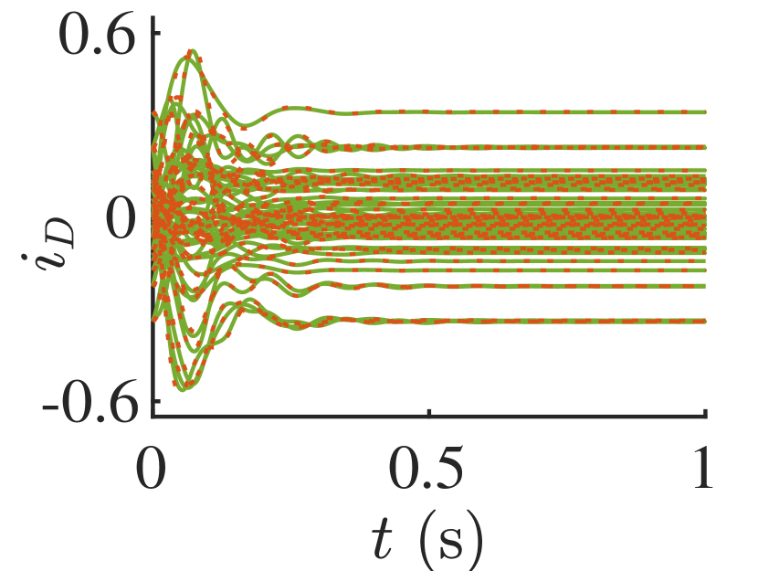
(c) ODE-Net performance at the final stage

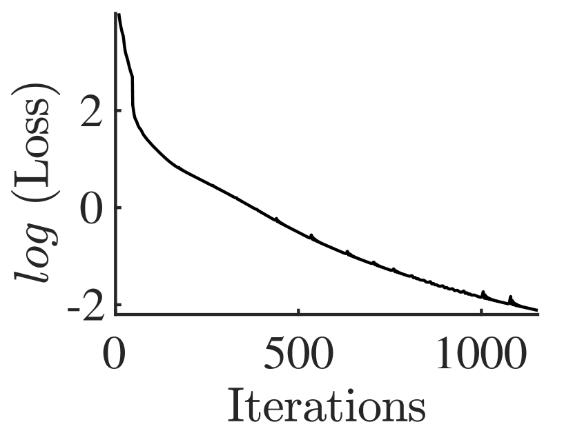
(d) Loss function evolution process

Figure 4: Training process of ODE-Net for NMs dynamic model discovery

Further, Fig. 5 illustrates the ODE-Net performance on the test set, which verifies its ability to generalize beyond the training set. Three types of scenarios are studied, i.e., no-fault, short-circuit fault, and open-circuit fault. A surprise finding is that the ODE-Net-enabled NMs formulation accurately captures the uncertain NMs transients not only under the frequently fluctuating DER uncertainties, but also under large disturbances, although the latter scenarios never appear in the training set. This shows the robustness of the ODE-net-enabled NMs formulation.

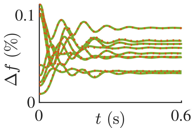
(a)

(b)

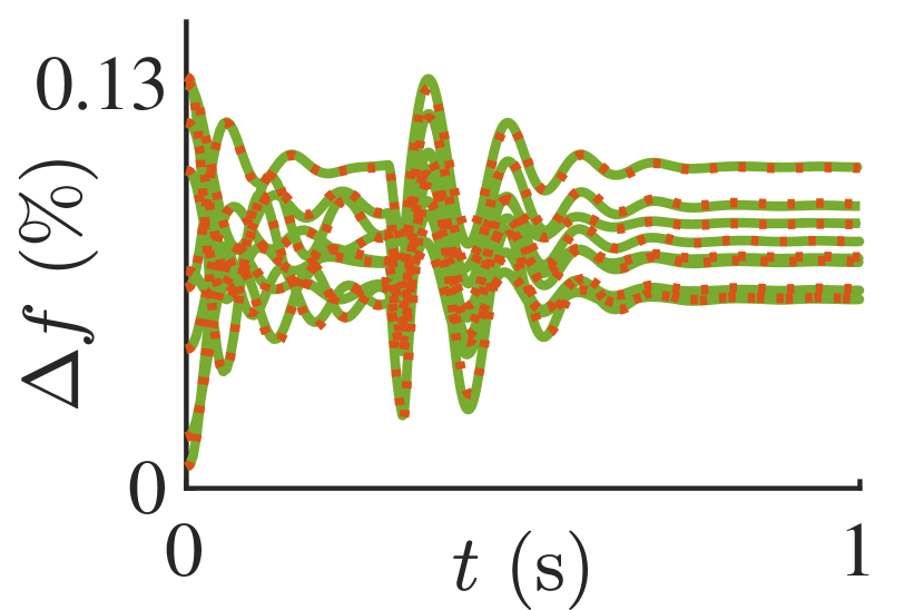
(c)

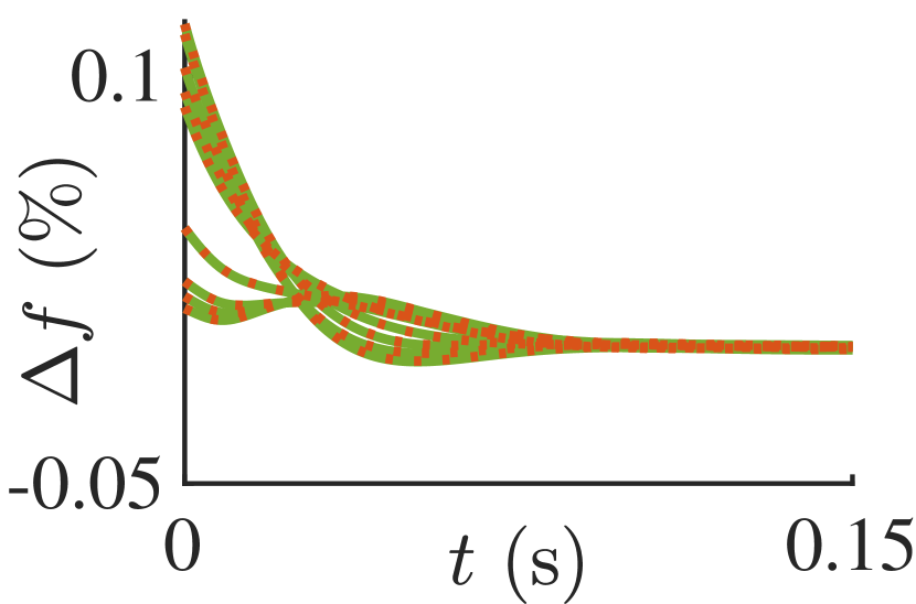
(d)

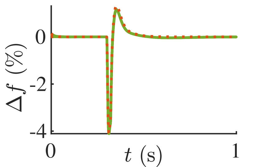
(e)

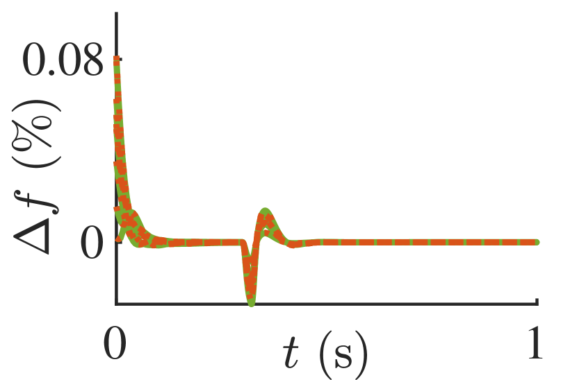
(f)

Figure 5: ODE-Net performance on the test set of NMs dynamics ($\Delta f$: frequency deviation). (a)-(c), droop control under no fault, short-circuit fault and open-circuit fault respectively. (d)-(f), secondary control under no fault, short-circuit fault and open-circuit fault respectively.

V-C NMs Dynamic Verification Via Neuro-Reachability

This subsection studies the NMs dynamics with both uncertain perturbations and fault disturbances via the Neuro-Reachability analysis.

Fig. 6 studies the neuro-reachsets under the quasi-static scenario, where the NMs is only perturbed by the DER uncertainties. The simulation shows that the neuro-reachsets tightly encloses the model-driven reachsets, which verifies both the accuracy and conservativeness of the method. In particular, in Case 2 where the DERs are equipped with secondary control, the Neuro-Reachability is supposed to learn not only the interactive currents between ExSys and InSys, but also the control signals from ExSys. Fig. 6(b) still shows a tight and perfect over-approximation of the real reachsets, which exhibits the potential of the Neuro-Reachability method in learning the NMs dynamic model with complicated hierarchy control. Neuro-Reachability shows the superiority of secondary control from two aspects: i) reachsets in Case 2 are narrower than the those in Case 1, which reflects strengthened robustness of the NMs against uncertainties; ii) reachsets in Case 2 get stable faster than those in Case 1, which reflects a speedy power sharing between the DERs during the NMs dynamics induced by uncertain perturbations.

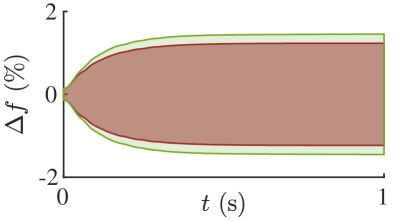
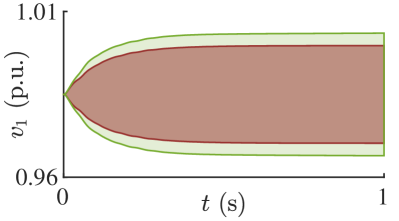
(a) Case 1: DERs with droop control

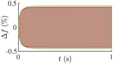
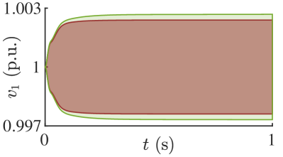
(b) Case 2: DERs with secondary control

Figure 6: Neuro-reachsets and its comparison with the model-driven reachsets ($\Delta f$: frequency deviation; $v_{1}$: voltage amplitude at DER1)

Further, Fig. 7 studies the neuro-reachsets under a momentary short-circuit fault occurred at 0.3s and cleared at 0.32s. Even though the ODE-Net-based NMs formulation is learned from the dynamics of small disturbances induced by the DERs’ uncertainties, simulation results show that the Neuro-Reachability method accurately and tightly captures the fast NMs dynamics under heterogeneous uncertainties during disturbances. Comparing the neuro-reachsets in Case 1 and Case 2, it is obvious that the secondary control exhibits restrained frequency/voltage dips and enhanced damping on the oscillations of the NMs states. Specifically, the reachable sets during the periods from the fault occurrence through the fault clearance are magnified by the subplots. Neuro-Reachability thus effectively mimics the NMs transients initiated by large disturbances.

(a) Case 1: DERs with droop control

(b) Case 2: DERs with secondary control

Figure 7: Neuro-reachsets under a short-circuit fault

V-D Efficacy and Versatility of Neuro-Reachability

This subsection studies the impact factors of the NMs reachsets via the Neuro-Reachability method.

V-D1 Neuro-Reachsets Under Different Uncertainty Levels

First, the impact of uncertainties on NMs dynamics is investigated. Taking DER1’s output-voltage in Case 2 as an example, Fig. 8 shows that the reachsets expand with the increasing uncertainties under both no-fault and faulted scenarios. The propagation of uncertainties in the NMs dynamics is therefore distinctly demonstrated by the neuro-reachsets at different uncertainty levels.

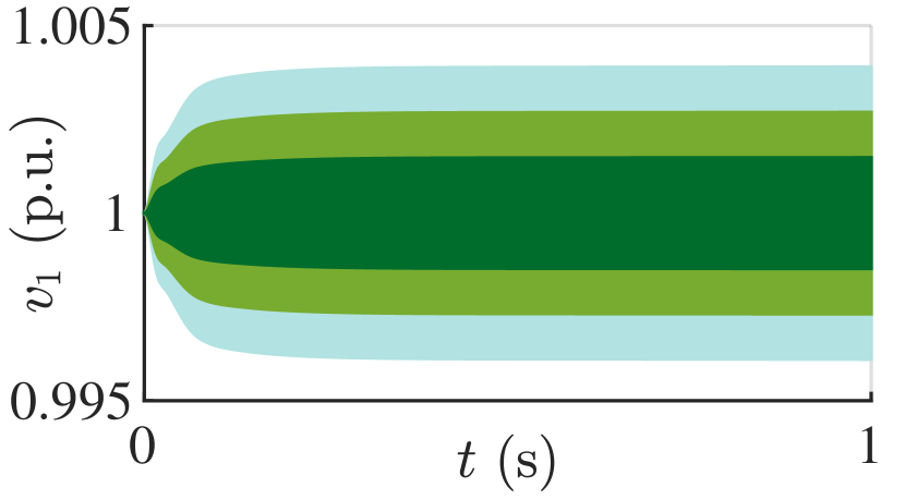
(a) No fault

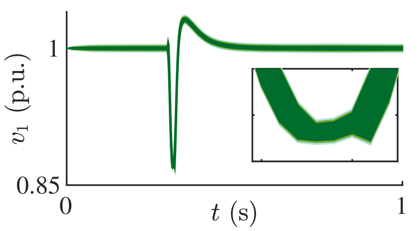
(b) Short-circuit fault

Figure 8: Neuro-reachsets under different uncertainty levels of Case 2

V-D2 Neuro-Reachsets Under Different Control Strategies

Second, the impact of the DERs’ control strategies on NMs reachsets is investigated. Fig. 6 and Fig. 7 exhibit the efficacy of the secondary control to stabilize the system under uncertainties from the time-domain perspective. Further, Fig. 9 presents the neuro-reachsets from a state-space observation. The efficacy of the secondary control for restraining the uncertainty impacts, damping the frequency/voltage overshoot and recovering the NMs states after faults are distinctly verified via the neuro-reachsets. Hence, Neuro-Reachability is promisingly helpful for verifying the controller’s performance under the infinite many uncertain scenarios in the absence of the microgrid model.

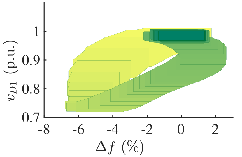
(a) Case 1: DERs with droop control

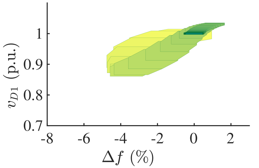
(b) Case 2: DERs with secondary control

Figure 9: State space neuro-reachsets under different control strategies

V-D3 Neuro-Reachsets Under Different Power Source Mixes

Finally, the impact of power source mixes is investigated via neuro-reachsets. Different power sources influence the NMs transients by their diverse dynamic features.

Fig. 10 studies the quasi-static reachsets (i.e., with no fault but only DER uncertainties perturbing the NMs) for Case 3, Case 4 and Case 5. The neuro-reachsets tightly encloses the model-driven reachsets in all cases, which again verifies the correctness of the Neuro-Reachability method. An interesting finding is that the neuro-reachsets of Case 3 in Fig. 10 are nearly identical to those of Case 1 in Fig. 6. This is because case 1 and Case 3 describe the identical NMs only with different microgrids being data-driven. Results of Case 4, compared with those of Case 3, show that the neuro-reachsets shrinks when the NMs are equipped with a SG, benefiting from the inertia and regulating ability of SG as well as its full dispachability compared with DERs. The neuro-reachsets is further improved when the NMs are equipped with an ESU as presented by the neuro-reachsets of Case 5, indicating enhanced robustness against the uncertainties with ESU. Meanwhile, it is noteworthy that both the SG and ESU provide voltage support to boost the NMs voltage, as illustrated in Fig. 10(b). Additionally, Fig. 11 investigates the neuro-reachsets of NMs during a short-circuit fault for Case 4 (i.e., equipped with a SG) and Case 5 (i.e., equipped with an ESU). The Neuro-Reachability method, as a data-driven approach, successfully captures the transient characteristics of the controllable power sources in restraining the uncertainties and damping the frequency/voltage dip/rise during the large disturbances compared with Fig. 9(a).

(a) Frequency reachset

(b) Voltage reachset

Figure 10: Neuro-reachsets under a short-circuit fault under different mixes of power sources in NMs

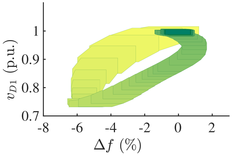
(a) Case 4

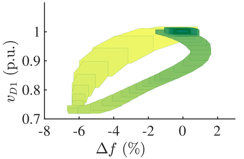
(b) Case 5

Figure 11: Neuro-reachsets under different mixes of power sources in NMs

VI Conclusions

This paper devises a Neuro-Reachability method, a data-driven approach to verify the uncertainty-disturbed, fast-changing and strongly-nonlinear dynamics of the NMs with unidentified subsystems. The ODE-Net-enabled dynamic model discovery, reachability analysis, and conformance theory conjointly enable a flexible and accurate model discovery of real-world microgrids, as well as provide reliable reachsets for verifying the NMs dynamics under heterogeneous uncertainties. Case studies of a typical NMs demonstrate the efficacy and robustness of the devised method. In the future, the Neuro-Reachability method will be enhanced for the dynamic verification of fully model-free NMs.

References

- [1] P. Zhang, Networked Microgrids. Cambridge University Press, 2020.
- [2] F. Feng and P. Zhang, “Enhanced microgrid power flow incorporating hierarchical control,” IEEE Transactions on Power Systems, vol. 35, no. 3, pp. 2463–2466, 2020.
- [3] W. Wan, M. Bragin, B. Yan, Y. Qin, J. Philhower, P. Zhang, and P. Luh, “Distributed and asynchronous active fault management for networked microgrids,” IEEE Transactions on Power Systems, 2020.
- [4] N. Soni, S. Doolla, and M. C. Chandorkar, “Improvement of transient response in microgrids using virtual inertia,” IEEE Transactions on Power Delivery, vol. 28, no. 3, pp. 1830–1838, 2013.
- [5] Y. Zhou, P. Zhang, and M. Yue, “Reachable dynamics of networked microgrids with large disturbances,” IEEE Transactions on Power Systems, under revision, May 2020.
- [6] T. A. Wilding, A. B. Gill, A. Boon, E. Sheehan, J.-C. Dauvin, J.-P. Pezy, F. O’beirn, U. Janas, L. Rostin, and I. De Mesel, “Turning off the drip (‘data-rich, information-poor’)–rationalising monitoring with a focus on marine renewable energy developments and the benthos,” Renewable and Sustainable Energy Reviews, vol. 74, pp. 848–859, 2017.
- [7] Y. Xu, Z. Y. Dong, L. Guan, R. Zhang, K. P. Wong, and F. Luo, “Preventive dynamic security control of power systems based on pattern discovery technique,” IEEE Transactions on Power Systems, vol. 27, no. 3, pp. 1236–1244, 2012.
- [8] Y. Zhou and P. Zhang, “Reachable power flow,” IEEE Transactions on Power Systems, vol. 35, no. 4, pp. 3290–3293, 2020.
- [9] Y. Zhou and P. Zhang, “Reachable eigenanalysis,” IEEE Transactions on Power Systems, 2020.
- [10] Y. Liu, K. Sun, R. Yao, and B. Wang, “Power system time domain simulation using a differential transformation method,” IEEE Transactions on Power Systems, vol. 34, no. 5, pp. 3739–3748, 2019.
- [11] Z. Yao, “A sufficient and necessary condition of transient stability for multimachine systems,” IEEE Transactions on Power Systems, vol. 35, no. 1, pp. 683–690, 2019.
- [12] H. Bosetti and S. Khan, “Transient stability in oscillating multi-machine systems using Lyapunov vectors,” IEEE Transactions on Power Systems, vol. 33, no. 2, pp. 2078–2086, 2017.
- [13] M. Korda and I. Mezić, “Linear predictors for nonlinear dynamical systems: Koopman operator meets model predictive control,” Automatica, vol. 93, pp. 149–160, 2018.
- [14] A. Surana and A. Banaszuk, “Linear observer synthesis for nonlinear systems using Koopman operator framework,” IFAC-PapersOnLine, vol. 49, no. 18, pp. 716–723, 2016.
- [15] S. Sinha, B. Huang, and U. Vaidya, “On robust computation of Koopman operator and prediction in random dynamical systems,” Journal of Nonlinear Science, pp. 1–34, 2019.
- [16] T. Guo and J. V. Milanović, “Online identification of power system dynamic signature using pmu measurements and data mining,” IEEE Transactions on Power Systems, vol. 31, no. 3, pp. 1760–1768, 2015.
- [17] C. Ren and Y. Xu, “A fully data-driven method based on generative adversarial networks for power system dynamic security assessment with missing data,” IEEE Transactions on Power Systems, vol. 34, no. 6, pp. 5044–5052, 2019.
- [18] L. Zheng, W. Hu, Y. Zhou, Y. Min, X. Xu, C. Wang, and R. Yu, “Deep belief network based nonlinear representation learning for transient stability assessment,” in 2017 IEEE Power & Energy Society General Meeting, pp. 1–5, IEEE, 2017.
- [19] T. Q. Chen, Y. Rubanova, J. Bettencourt, and D. K. Duvenaud, “Neural ordinary differential equations,” in Advances in neural information processing systems, pp. 6571–6583, 2018.
- [20] I. Goodfellow, Y. Bengio, and A. Courville, Deep Learning. MIT Press, 2016. http://www.deeplearningbook.org.
- [21] Y. Sun, L. Zhang, and H. Schaeffer, “NeuPDE: Neural network based ordinary and partial differential equations for modeling time-dependent data,” arXiv preprint arXiv:1908.03190, 2019.
- [22] Y. Zhou, P. Zhang, and M. Yue, “An ODE-enabled distributed transient stability analysis for networked microgrids,” in 2020 IEEE Power and Energy Society General Meeting (PESGM), Montreal, Quebec, Canada, 2020.
- [23] M. Althoff and B. H. Krogh, “Zonotope bundles for the efficient computation of reachable sets,” in 50th IEEE Conference on Decision and Control, pp. 6814–6821, 2011.
- [24] M. Althoff, O. Stursberg, and M. Buss, “Reachability analysis of nonlinear systems with uncertain parameters using conservative linearization,” in 47th IEEE Conference on Decision and Control, pp. 4042–4048, 2008.
- [25] S. B. Liu and M. Althoff, “Reachset conformance of forward dynamic models for the formal analysis of robots,” in 2018 IEEE/RSJ International Conference on Intelligent Robots and Systems (IROS), pp. 370–376, IEEE, 2018.
- [26] N. Kochdumper, A. Tarraf, M. Rechmal, M. Olbrich, L. Hedrich, and M. Althoff, “Establishing reachset conformance for the formal analysis of analog circuits,” in 2020 25th Asia and South Pacific Design Automation Conference (ASP-DAC), pp. 199–204, IEEE, 2020.
- [27] N. Pogaku, M. Prodanovic, and T. C. Green, “Modeling, analysis and testing of autonomous operation of an inverter-based microgrid,” IEEE Transactions on Power Electronics, vol. 22, no. 2, pp. 613–625, 2007.
- [28] D. P. Kingma and J. Ba, “Adam: A method for stochastic optimization,” arXiv preprint arXiv:1412.6980, 2014.