The polar precursor method for solar cycle prediction: comparison of predictors and their temporal range

Abstract

The polar precursor method is widely considered to be the most robust physically motivated method to predict the amplitude of an upcoming solar cycle. It uses indicators of the magnetic field concentrated near the poles around sunspot minimum. Here, we present an extensive performance analysis of various such predictors, based on both observational data (WSO magnetograms, MWO polar faculae counts and Pulkovo $A(t)$ index) and outputs (polar cap magnetic flux and global dipole moment) of various existing flux transport dynamo models. We calculate Pearson correlation coefficients ($r$) of the predictors with the next cycle amplitude as a function of time measured from several solar cycle landmarks: setting $r=0.8$ as a lower limit for acceptable predictions, we find that observations and models alike indicate that the earliest time when the polar predictor can be safely used is 4 years after polar field reversal. This is typically 2–3 years before solar minimum and about 7 years before the predicted maximum, considerably extending the usual temporal scope of the polar precursor method. Re-evaluating the predictors another 3 years later, at the time of solar minimum, further increases the correlation level to $r\gtrsim 0.9$. As an illustration of the result, we determine the predicted amplitude of Cycle 25 based on the value of the WSO polar field at the now official minimum date of December 2019 as $126\pm 3$. A forecast based on the value in early 2017, 4 years after polar reversal would have only differed from this final prediction by $3.1\pm 14.7$%.

1. Introduction

The Sun’s magnetic field increases and decreases in time with a polarity reversal every 11 years. This cycle of magnetic field is widely studied using the sunspot number and areas as they are the signatures of the strong field and are available for a longer duration than the direct observations of the surface magnetic field, which are available in the form of synoptic maps only since around 1955s. The strength of the solar magnetic field, however, varies from cycle to cycle in an irregular manner (Hathaway, 2015). The Maunder minimum, an extended period of weaker field, is an extreme example of such irregular behaviour. It is this variable magnetic field that drives the fluctuations of the solar wind and terrestrial space weather, which may have hazardous effects on human activities that depend on the stability of our magnetospheric environment (space missions, satellites, telecommunications, etc.). To assess and prevent those risks, reliable predictions of future solar activity are now more than ever essential.

Many attempts have been made to predict an upcoming solar cycle based on the extrapolation of the time series of some proxy of solar activity. However, most of the time, they produce diverging results (Pesnell, 2012).

Predictions of the solar cycle based on dynamo theory have also been made (Petrovay, 2020). In most dynamo models, the polar magnetic field is a natural predictor of the following cycle. Indeed, there is considerable evidence that the solar dynamo is a magnetohydrodynamical $\alpha\omega$-dynamo (Charbonneau, 2010) where the strong toroidal field, manifest in the form of sunspots, is generated by the winding up of a weaker poloidal magnetic field by differential rotation. This windup is essentially a linear process; hence the amplitude of a solar cycle is expected to be proportional to the amplitude of the poloidal field around the start of the cycle. As this poloidal field is strongly concentrated to the poles, the amplitude of the polar surface magnetic field is a plausible measure of its amplitude.

Following this idea, Schatten et al. (1978) used the polar field strength at the solar minimum to make the first prediction of the sunspot number during Cycle 21. Later this idea was validated by many authors using different proxies of the polar field, such as $aa$-index, polar faculae, and active networks (Makarov et al., 1989; Choudhuri et al., 2007; Jiang et al., 2007; Wang & Sheeley, 2009; Kitchatinov & Olemskoy, 2011; Muñoz-Jaramillo et al., 2013; Priyal et al., 2014). Furthermore, surface flux transport models, which provide the evolution of the surface radial field by utilizing the observed BMRs and large-scale flows have also been used to predict the amplitude of the upcoming solar cycle (Iijima et al., 2017; Jiang et al., 2018; Upton & Hathaway, 2018).

As a whole, predictions based on these polar precursors tend to yield much more consistent results than time series methods, and there is now wide consensus that this is the most robust physically motivated method to predict the amplitude of an upcoming solar cycle.

However, when applying polar precursor methods, a variety of choices need to be made regarding the measures or proxies of the poloidal field to use, and the exact time at which they are evaluated. The purpose of the present work is to make a systematic analysis of the performance of various such predictors and determine a temporal window when their evaluation is optimal. Some of the questions we address are: Is it the polar field at the time of its peak value that best determines the strength of the next cycle or is it at a different time? Is there an acceptable window over which we can use the polar field data to make a prediction? Do we need to wait until the activity minimum to make a reliable prediction of the next cycle?

Table 1Relative time shifts (in years) between different solar cycle landmarks: observations and models.

	Observations
Shift between
$t_{{\rm SSA,min},i}$ to $t_{{\rm SSA,min},i+1}$	10.83$\pm$0.83
$t_{{\rm SSA,min},i}$ to $t_{{\rm SSA,max},i}$	4.58$\pm$0.81
	Faculae		PF		DM		$A(t)$ index
$t_{{\rm SSA,min},i}$ to $t_{{\rm p,rev},i}$	5.01$\pm$0.64		4.12$\pm$0.36		3.53$\pm$0.27		3.55$\pm$0.48
$t_{{\rm SSA,max},i}$ to $t_{{\rm p,max},i}$	5.93$\pm$1.89		4.40$\pm$0.99		1.84$\pm$0.80		4.85$\pm$1.47
$t_{{\rm p,max},i-1}$ to $t_{{\rm SSA,max},i}$	4.64$\pm$1.18		5.78$\pm$1.89		7.88$\pm$2.43		5.66$\pm$1.26
$t_{{\rm p,rev},i}$ to $t_{{\rm p,max},i}$	5.76$\pm$1.49		5.48$\pm$0.74		3.52$\pm$1.16		4.96$\pm$0.78
$t_{{\rm p,rev},i}$ to $t_{{\rm SSA,min},i+1}$	5.60$\pm$1.01		6.81$\pm$1.53		7.39$\pm$1.34		6.88$\pm$0.61
$t_{{\rm p,max},i-1}$ to $t_{{\rm SSA,min},i+1}$	10.72$\pm$1.45		10.94$\pm$2.28		12.92$\pm$3.42		12.08$\pm$1.28

	Models
	2DR1		3DR1			2$\times$2D-R1
Shift between	PF	DM		PF	DM		PF		DM
$t_{{\rm SSN,min},i}$ to $t_{{\rm SSN,min},i+1}$	11.12$\pm$1.26	$---$		10.50$\pm$0.74	$---$		10.25$\pm$0.93		$---$
$t_{{\rm SSN,min},i}$ to $t_{{\rm SSN,max},i}$	5.76$\pm$0.53	$---$		5.29$\pm$0.47	$---$		$4.92\pm$0.83		$---$
$t_{{\rm SSN,min},i}$ to $t_{{\rm p,rev},i}$	4.36$\pm$0.41	4.96$\pm$0.52		5.52$\pm$0.47	4.54$\pm$1.62		3.10$\pm$0.72		2.67$\pm$0.67
$t_{{\rm SSN,max},i}$ to $t_{{\rm p,max},i}$	3.98$\pm$0.94	4.78$\pm$0.96		5.40$\pm$1.10	3.71$\pm$1.37		2.57$\pm$1.52		2.47$\pm$1.28
$t_{{\rm p,max},i-1}$ to $t_{{\rm SSN,max},i}$	7.14$\pm$1.26	6.44$\pm$1.24		5.08$\pm$0.99	6.79$\pm$1.26		7.70$\pm$1.52		7.79$\pm$1.29
$t_{{\rm p,rev},i}$ to $t_{{\rm p,max},i}$	5.74$\pm$1.14	5.62$\pm$0.98		5.31$\pm$1.05	4.49$\pm$1.47		4.38$\pm$1.33		4.72$\pm$1.12
$t_{{\rm p,rev},i}$ to $t_{{\rm SSN,min},i+1}$	6.75$\pm$1.03	6.26$\pm$0.93		4.98$\pm$0.55	5.98$\pm$1.30		7.14$\pm$0.92		7.58$\pm$0.73
$t_{{\rm p,max},i-1}$ to $t_{{\rm SSN,min},i+1}$	12.47$\pm$1.92	11.86$\pm$1.89		10.16$\pm$1.09	12.05$\pm$1.41		13.02 $\pm$ 1.44		13.10$\pm$1.24

In Section 2 these questions are considered on the basis of the available observational data. This analysis leads to some interesting findings, the most important of which is that the temporal scope of the polar precursor method is longer than generally thought: reliable predictions can be made already 4 years after the reversal of the Sun’s polar magnetic field, that is on average 3 years before the minimum and 7 years before the next maximum. This significant extension of the temporal scope of the polar precursor method is potentially highly relevant for solar cycle prediction efforts.

As, however, it is based on observational data covering only a limited number of solar cycles, the statistical robustness of this result may reveal somewhat doubtful. Hence, in Section 3 we extend our analysis to some dynamo models that have been calibrated to represent reasonably well the observed spatiotemporal variation of solar activity. As in these models a higher number of cycles can be simulated, in this case the size of the statistical sample is not a concern. On the other hand, the three dynamo models considered are different in their construction and in the parameter range where they operate, so a direct comparison of the models with each other or with the real Sun is questionable. Hence, we focus here only on those results where all models agree with each other and the observations, and consider these as robust and independent of model details.

As we conclude in Section 4, the possibility to predict an upcoming cycle on the basis of a measure of the poloidal field 4 years after the observed time of polar reversal is found to be one such robust result. To illustrate the result, in the Conclusions we also compare predictions of Cycle 25 that could have been made 4 years after polar reversal, i.e. in early 2017, to those based on the polar field amplitude at the now official date (December 2019) for the start of the new cycle.

Throughout the paper, we will use the generic symbolic notation $P$ for the different predictors (poloidal field measures) considered, and $T$ for the predicted variable characterizing the solar activity level (e.g. sunspot area, sunspot number or toroidal field amplitude).

2. Observational data analysis

2.1. Data

For observational measures and proxies of the solar poloidal field $P$, we consider polar field strength and global dipole moment values derived from Wilcox Solar Observatory (WSO) magnetic field measurements for the last four cycles (1974–2019); Mt. Wilson Observatory (MWO) polar faculae counts for the last ten cycles (1907–2011); and Pulkovo Observatory $A(t)$ index series for the period 1915–1999.

The monthly time series of WSO polar magnetic field data, smoothed using a Gaussian filter with FWHM = 6 months (Hathaway et al., 2002), is denoted here by $B_{N}(t)$ and $B_{S}(t)$ for the Northern and Southern hemispheres, respectively. As a further possible predictor we also consider the global solar dipole moment defined as

$${\rm DM}(t)=\frac{3}{2}\int_{-\pi/2}^{\pi/2}B(\lambda,t)\sin\lambda\cos\lambda\,\mathrm{d}\lambda,$$ (1)

where $\lambda$ is the heliographic latitude and $B=\frac{1}{2\pi}\int_{0}^{2\pi}B_{r}\,d\phi$ is the azimuthally averaged field strength. Values of ${\rm DM}(t)$ computed using this formula with WSO data for the period 1976–2017 were kindly provided to us by Jie Jiang (Jiang et al., 2018).

The polar faculae count is considered a proxy of the polar field as they share a significant correlation (Sheeley, 1991). The MWO faculae counts used here were determined by Muñoz-Jaramillo et al. (2012).

The $A(t)$ index, representing the sum of the intensities of dipole and octupole components of the Sun’s large-scale magnetic field, as reconstructed on the basis of Pulkovo H_α synoptic maps, is obtained from Makarov et al. (2001). Since this index does not include the quadrupolar component, symmetric to the equator, it is expected to scale roughly with the antisymmetric part of the polar fields, $(B_{N}-B_{S})/2$.

To characterize the amplitude of solar cycles, we use the peak of the sunspot area (SSA) distribution obtained from the Greenwich Royal Observatory, smoothed using a Gaussian filter of FWHM $=12$ months.

2.2. Solar cycle landmarks

We consider two types of landmarks during a solar cycle to which the time of evaluation of the precursor $P$ can be bound: the maxima (or minima) of the smoothed sunspot area (SSA), from which we measure backward delays, and the time of reversal (zero crossing) of the various poloidal field indicators $P$, from which we measure forward delays. The relative time shifts between these landmarks varies from cycle to cycle; their average values are collected in Table 1 for later reference. We note that in the polar faculae data, the epochs of polar field reversal is not available, and thus we take these as the same as the time of minima of the faculae.

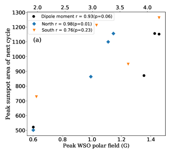
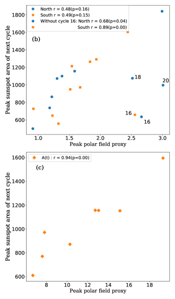
Figure 1.— Scatter plot of the peak value of the polar field (or its proxy) vs the peak sunspot area in the following cycle for (a) WSO polar field and dipole moment (Cycles 21 to 24), (b) MWO polar faculae (Cycles 14 to 23), and (c) Pulkovo Observatory $A(t)$ index (Cycles 15 to 22). Sunspot areas in (a) and (b) are hemispheric peak values, while in (c) the peak value of the hemispheric average.

2.3. Correlations in the observed data

Scatter plots of the peak values of various measures or proxies of the poloidal field $P$ against the amplitude of the following sunspot cycle are shown in Figure 1. We note that Pearson correlations are given here and throughout this paper.

While the correlation is high in the WSO data (Figure 1(a)), it is less impressive in faculae data (Figure 1(b)). Particularly, in the northern hemisphere, the correlation is relatively poor because of Cycles 16, 18, and 20. Note that faculae counts for Cycle 16 may be problematic, as already noted by Priyal et al. (2014). If we exclude only Cycle 16, then the correlation considerably improves. Figure 1(c) shows that the $A(t)$ index, available for the longest time interval of all the considered polar field measures, performs quite well as a predictor. This is somewhat surprising, given that the index is based on a very rough reconstruction of the large scale solar magnetic fields: a simple two-valued function ($+1$ or $-1$, constant in each unipolar zone outlined by the neutral lines reconstructed from the available H_α synoptic maps).

We note that the time when a given $P$ peaks may differ from the sunspot cycle minimum by several years. Usually, the $P$ proxies peak one to two years before the sunspot cycle minimum. Hence, evaluating $P$s at solar minimum yields somewhat different values for these correlations, which are nevertheless found to be similar to the values for peak $P$s shown in Figure 1. When evaluated at sunspot minimum, the correlation values are, respectively for the northern and southern hemisphere, $r=0.86$ ($p=0.14$) and $r=0.86$ ($p=0.14$) for the WSO polar field data, and $r=0.60$ ($p=0.06$) and $r=0.66$ ($p=0.04$) for the MWO facular data —comparable to those reported in Muñoz-Jaramillo et al. (2012) from the same facular data.

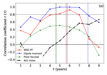
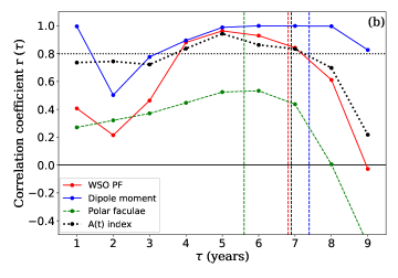
Figure 2.— Pearson’s correlation coefficient $={\rm Corr}[T(t_{\rm max}),P(t)]$ between the peak sunspot area $T$ at the maximum of the next cycle and polar field measures $P(t)$ as a function of time (a) measured backward from the cycle maximum: $t=t_{\rm max}-\tau$, (b) measured forward from the reversal of $P$: $t_{\rm rev}+\tau$. Vertical lines indicate the average positions of other cycle landmarks in the given plot, with the same color coding as the associated curves. (a) Black dots: cycle minimum $T_{{\rm SSA,min},i}$, dashed lines: time shift from the time of the maximum of $|P|$ to next cycle maximum $T_{{\rm p,max},i-1}\rightarrow T_{{\rm SSA,max},i}$. (b) Dashed lines: time shift from reversal of $P$ to cycle minimum $T_{{\rm p,rev},i-1}\rightarrow T_{{\rm SSA,min},i}$.

To proceed towards the main purpose of this analysis, we now consider the time dependence of these correlations. Figure 2 shows the correlation coefficient values against time $\tau$ (in years) measured from two different solar cycle landmarks: backward from solar maximum and forward from poloidal field reversal. The curve labeled WSO here shows the WSO polar field results.

For WSO and polar facular data the correlations are calculated based on a data set consisting of the hemispheric values of the polar field vs the hemispheric amplitude of the next cycle, for both hemispheres in the same data set. This effectively doubles the sample size.

The curves obtained are not smooth, presumably due to the limited sample size (limited number of cycles). Nevertheless, it is apparent that both panels display a 3–4 year long plateau where correlation values are consistently high. This is the reason why no significant difference was found above, between correlation levels for predictors evaluated at cycle minimum or at the time when they take their peak values.

The plateaus further suggest that the polar precursor may give reliable predictions at times significantly earlier than solar minimum. Indeed, Figure 2(a) shows that WSO magnetic field data may correctly predict the amplitude of the next cycle maximum up to 7 years ahead —that is a few years earlier than either the cycle minimum or the time when the polar field measures typically reach their maxima.

While this long temporal range of the polar precursor method is an important finding, for practical applications the precursor needs to be evaluated at a time measured forward from an already known landmark, rather than backward from an as yet unobserved one. Hence, in Figure 2(b) the correlations are now plotted against time measured forward from the reversal of the given poloidal field measure $P$. It is again apparent that reliable predictions, at a Pearson correlation level above 0.8, may be possible already 4 years after polar reversal, that is on average 3 years before cycle minimum.

Regarding the possible choices of precursors $P$, we see that polar faculae counts are clearly inferior to other $P$s, including the $A(t)$ index. Note, however, that omitting Cycle 16 can significantly improve their performance, as discussed above. The performance of the WSO polar field correlations and of the global dipole moment are comparable.

These results indicate that the temporal range of the polar precursor method is longer than it is generally thought and that reliable predictions based on this method can be made 4 years after polar reversal, which is, on average, nearly 3 years earlier than cycle minimum and 7 years before the predicted maximum. In reality, this temporal range may be even longer and a prediction may be made even earlier just by seeing how rapidly the polar field is growing. As shown in Appendix, there is some correlation between the rise rate of the polar field and the amplitude of the next cycle.

As, however, the statistical sample size upon which these conclusions are based is limited, for further support we turn to dynamo models that are capable to simulate a larger number of solar cycles than those few that have been well observed.

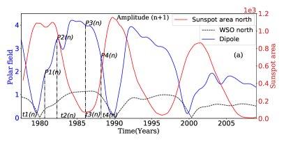
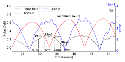
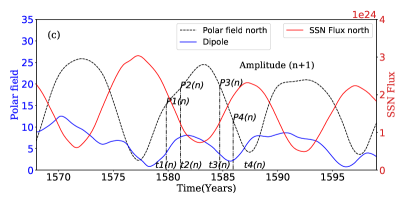
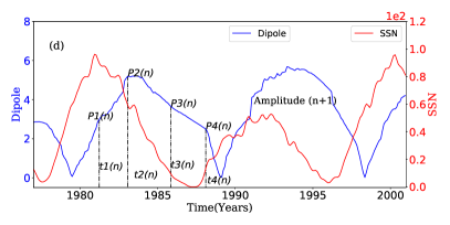
Figure 3.— Time series of some predictors $P$ (blue and black) and predicted activity indicators $T$ (red). (a) Observations; (b) Surya 2DR1 model; (c) STABLE 3DR1 model; (d) 2$\times$2D-R1 model. Some example intervals used for the determination of rise and decay rates (see Appendix) of $P$ are marked. Rise and decay rates in cycle $n$ are defined as $(P2(n)-P1(n))/(t2(n)-t1(n))$ and $(P4(n)-P3(n))/(t4(n)-t3(n))$, respectively.

3. The polar precursor in solar dynamo models

It is now understood that intercycle fluctuations in solar activity are due to fluctuations in the amplitude of the poloidal field that serves as a seed for the strong toroidal field in the next cycle. Fluctuations in the poloidal field, in turn, arise as a consequence of the stochastic nature of flux emergence that, upon the action of surface flux transport processes, ultimately gives rise to the polar fields. This is the so-called Babcock–Leighton mechanism. To simulate intercycle variations two approaches are therefore open: to introduce stochastic variations directly into the poloidal component of the dynamo equations (Charbonneau & Dikpati 2000, Karak & Choudhuri 2011, Kitchatinov et al. 2018, Cameron & Schüssler 2017) or to explicitly incorporate the stochastic flux emergence process into the model (Yeates & Muñoz-Jaramillo 2013, Miesch & Dikpati 2014, Lemerle & Charbonneau 2017, Bhowmik & Nandy 2018). By calibrating the numerous parameters of these models it is possible to tune them to resemble the observed solar cycle in their behaviour, which opens the possibility that assimilating past observed behaviour into the models and considering future stochastic variations in an ensemble forecast approach, they may be used for the prediction of upcoming solar cycles. Some forecasts for Cycle 25 have indeed been presented using this approach (Bhowmik & Nandy 2018, Labonville et al. 2019).

In this section we will use three such models to investigate the relative merits of different measures $P$ of the poloidal field as cycle precursors and their time span. All these models are kinematic flux transport dynamos and thus the large-scale flows, such as meridional circulation and differential rotation are imposed as guided by observations. While the differential rotation profile is the same in all the models, the meridional circulation is somewhat different.

One model, Surya (Chatterjee et al., 2004) belongs to the first class mentioned above, with stochastic fluctuations introduced directly to the polar field, while the other two models, STABLE (Karak & Miesch, 2017) and 2$\times$2D (Lemerle & Charbonneau, 2017) explicitly incorporate randomized individual active region sources.

Before discussing each model individually, it is instructive to consider how they fare in reproducing the observed time shifts between solar cycle landmarks. These time shifts are collected in Table 1 (to be compared with the observed values above), while the time profiles of some of the relevant precursors and activity indicators are shown in Figure 3. A closer comparison between the model outputs and the observations leads to a somewhat disappointing conclusion: despite their respective calibration to specific characteristics of solar observations, many of the relative phases and time shifts presented in Table 1 are not properly reproduced by any of the three models.

To start with, none of the models reproduce enough asymmetry in its cycle profiles: maxima fall at a phase of 0.48–0.52 in contrast to the observed value of 0.42. The timing of polar field reversals is also out of phase. In Surya 2DR1, the polar field reverses earlier than the dipole moment (Fig. 3b), in contrast to observations. In STABLE 3DR1 the average time of the reversal is too late by more than a year and its timing, especially for the dipole moment, shows very wide haphazard intercycle variations. In the 2$\times$2D model the reversal is about a year earlier than observed and tends to fall in the middle of the rising phase of the cycle.

The reason for these discrepancies is mainly that the calibration of the models to observations is usually judged by a (quantitative or qualitative) agreement between the observed and modeled shapes of the activity butterfly diagram and of the supersynoptic map of the poloidal field evolution. As the polar areas cover a small fraction of the solar surface, they do not weigh much in such comparisons; and a comparison to temporal profiles of activity is often not impelled (see also Petrovay & Talafha 2019).

Facing these irregularities we embark in our study of the performance of polar precursors in dynamo models with reserve. What we are looking for is whether, despite their imperfect optimizations, their simplifications, their physical differences and the different parameter regimes in which they operate, there are any features where the behaviour of possible polar precursors agrees in all the models and observations.

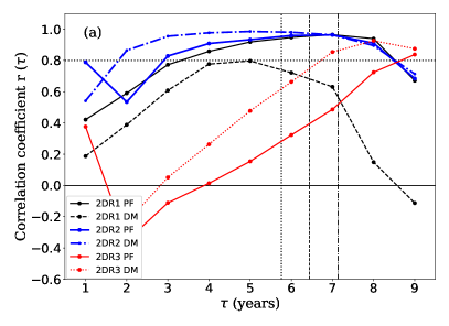
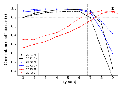
Figure 4.— Same as Fig. 2, for different parameterizations of the Surya dynamo model. PF: polar cap flux; DM: global dipole moment. Vertical lines mark the mean positions of cycle landmarks with the same colour coding as the associated curves. (a) Black dots: cycle minimum $T_{{\rm SSN,min},i}$, dashed lines: time shift from the time of the maximum of $|P|$ to next cycle maximum $T_{{\rm p,max},i-1}\rightarrow T_{{\rm SSN,max},i}$. (b) Dashed and dot dashed lines show the time shift from reversal of $P$ to cycle minimum $T_{{\rm p,rev},i-1}\rightarrow T_{{\rm SSN,min},i}$, respectively for dipole moment and polar field.

3.1. Surya dynamo model

Surya is an axisymmetric dynamo model in which equations for the poloidal and toroidal fields are solved numerically. Diffusivity for the poloidal magnetic field in the whole CZ is $3\times 10^{12}$ cm² s^-1. In contrast, below the radius of $0.975R_{\odot}$ the diffusivity for the toroidal component is reduced to $4\times 10^{10}$ cm² s^-1. While the detailed model was presented in Chatterjee et al. (2004), over the years some parameters have been changed in order to make a closer comparison with observations (Karak, 2010; Hazra et al., 2015; Karak et al., 2018). For the present study we use the version of the code that was used in Karak & Choudhuri (2011).

The basic Surya model tends to produce a regular magnetic cycle. However, the variations in the Babcock–Leighton process and meridional flow can produce variations in the magnetic cycle. Karak & Choudhuri (2011) showed that a combination of $100\%$ fluctuations with a coherence time of one month in the Babcock–Leighton $\alpha$ and $30\%$ in the meridional flow with a coherence time of 30 years could produce variations in the solar cycle comparable to that seen in the observed solar cycle and successfully explain the Waldmeier effect. We perform a first run with this combination of fluctuations, labelled 2DR1. We then perform two more runs for comparison: run 2DR2 is identical to 2DR1 but with the strength of the Babcock–Leighton $\alpha$ increased by a factor 2; and run 2DR3 is identical to 2DR1 but with the diffusivity of the poloidal field reduced by half.

Activity level $T$ in the model is characterized by the toroidal flux at $10^{\circ}\leq$ latitude $\leq 30^{\circ}$ at $r=0.71R_{\odot}$. For the precursor $P$, the polar cap flux PF (surface flux poleward of latitude $75^{\circ}$) and the global dipole moment DM are considered. The time variation of the correlation between $P$ and $T$ is displayed in Figure 4.

While the low diffusivity run 2DR3 is clearly off, it is seen that the run 2DR2, with elevated poloidal source term, actually produces higher correlations than the reference case 2DR1. In 2DR2 both PF and DM are found to be good predictors of the upcoming cycle amplitude while in 2DR1 for DM this is only true when time is measured from the reversal. Nevertheless, PF and DM are found to be very good predictors of an upcoming solar maximum right from the time of reversal (panel (b)) for both runs, with optimal performance of the predictor reached around cycle minimum.

Some conclusions about the physics of the model versus the real Sun may also be drawn from these plots. The fact that the correlation in panel (a) becomes strong for about $\tau>4$ years in the first two runs suggests that the polar field needs at least 4 years to be transported to the base of the CZ and produce toroidal field for the next cycle. Keeping in mind the diffusivity of the poloidal field ($3\times 10^{12}$ cm² s^-1), the diffusion time for the poloidal field to reach from the surface to the base of CZ is $4.6$ years. Thus, the delay time in the correlation in Figure 4(a) for runs 2DR1 and 2DR2 is reasonable. As the average time delay from polar reversal is around 6 years, the correlation is good already very soon after the time of reversal, in contrast to observations. This suggests that Surya runs 2DR1 and 2DR2 operate in a somewhat more diffusive regime than the solar dynamo. In agreement with this, the very low diffusivity run 2DR3 deviates starkly from observations. There is a weak negative correlation between $P$ and $T$ for $\tau<7$ years. Then it increases to positive values at large $\tau$. This clearly shows that in this run, the model needs at least about 8 years for the polar flux from the previous cycle to be transported to the deep CZ to produce strong toroidal flux. The reason for this delay correlation is the lower diffusivity. In this case, the diffusivity for the poloidal field is $1.5\times 10^{12}$ cm² s^-1 and thus the diffusion time is 9.2 years, which is double than that in runs 2DR1 and 2DR2. This explains the strong positive correlation in Run 2DR3 for $\tau>8$ years.

3.2. STABLE dynamo model

The STABLE (Surface flux Transport And Babcock–Leighton) dynamo model was originally developed by Mark Miesch and his colleagues at High Altitude Observatory (Miesch & Dikpati, 2014; Miesch & Teweldebirhan, 2016). Later this model was significantly improved by Karak & Miesch (2017) to make a close connection of the BMR eruption and evolution on the surface with observations. The salient features of this model are the following. (i) It is a full 3D dynamo model in which the induction equation is solved over the whole solar CZ. Unlike the Surya model, the turbulent diffusivity for all components of magnetic fields is the same. The diffusivity has a radial dependent profile such that in the CZ it has a value of about $10^{12}$ cm² s^-1 ($4.5\times 10^{12}$ cm² s^-1 for $r>0.956R_{\odot}$ and $1.5\times 10^{12}$ cm² s^-1 below) and below the CZ it drops by about four orders of magnitude. The model includes a radial downward magnetic pumping with a speed 20 m s^-1 in the top $10\%$ of solar radius to mimic the asymmetric convection. (ii) Timing of BMR eruption: This model places a BMR only when certain conditions are satisfied. First, the magnetic field at the base of the CZ must exceed a critical field strength. Second, after the first BMR is produced, the time for the second BMR will be taken from a log-normal distribution which is obtained from the observations of BMRs. (iii) Connecting the toroidal field to BMR: The rate of BMR production is regulated with the strength of the magnetic field such that when the magnetic field in the base of the CZ is strong it produces a large number of BMRs. Thus the delay distribution is regulated by the magnetic field and it is the only part through which, the toroidal field is linked to the BMRs (and thus the poloidal field) in this model. (iv) While the magnetic field in BMR is fixed at 3 kG, the flux is obtained from the observed distribution. The tilt is obtained from Joy’s law with a Gaussian scatter around it. A magnetic field dependent nonlinear quenching is imposed in the tilt to saturate the magnetic field in this dynamo model. We note that recently some evidence of nonlinear quenching in the tilt is observed in the BMR data (Jha et al., 2020). As shown in Jiang (2020) and Karak (2020), the observed latitude variation of BMRs provides another nonlinearity to stabilize the magnetic cycles in Babcock–Leighton dynamos. In addition to the tilt quenching, this nonlinearity is also operating in the model to limit the amplitudes of the magnetic cycles. For further details of the STABLE dynamo model, we refer the reader to Sections 2 and 4 of Karak & Miesch (2017).

From the simulation presented in Karak & Miesch (2017), we take the runs B10, B11 and B13 as listed in their Table 1. We relabelled them here as 3DR1, 3DR2, and 3DR3, respectively. In run 3DR1, a Gaussian scatter of zero mean and $\sigma=15^{\circ}$ is included around Joy’s law, while in run 3DR2, the scatter is doubled i.e., $\sigma=30^{\circ}$. Finally, run 3DR3 is the same as run 3DR1, except that the diffusivity below the CZ is made the same as that in the CZ ($1.5\times 10^{12}$ cm² s^-1).

Activity level $T$ in the model is characterized by the total monthly flux in emerging BMRs. For the precursor $P$, the polar cap flux PF (surface flux polewards of latitude $75^{\circ}$) and the global dipole moment DM are considered. The time variation of the correlations between $P$ and $T$ is displayed in Figure 5.

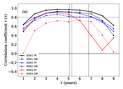
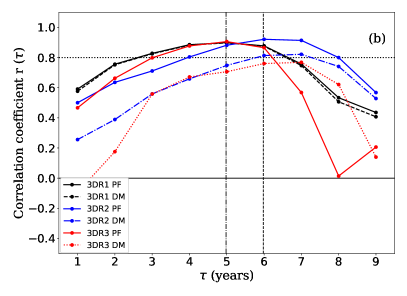
Figure 5.— Same as Fig. 4, for different parameterizations of the STABLE dynamo model.

In the reference run 3DR1, both PF and DM are found to be very good precursors of the next cycle amplitude over a broad temporal range starting 7 years before the predicted maximum or 4 years after polar reversal. This agrees well with observations. One interesting aspect of panel (a) is that the correlation exceeds about 0.8 already at $\tau\sim 2$–$3$ years, implying that the poloidal flux reaches the deep CZ more quickly in these runs than in the Surya runs. While the diffusivity in the STABLE model is comparable to that of the Surya model, a downward magnetic pumping in the top $10\%$ of the CZ is an additional agent for transporting the poloidal flux from the surface to the deep CZ. This downward pumping may help to produce a strong correlation in panel (a) even at small $\tau$ (panel (b) at large $\tau$).

Run 3DR2, with increased stochasticity, produces somewhat lower correlations, as expected. On the other hand, in panel (a) agreement with observations is improved for larger values of $\tau$ (more rapid fall for $\tau>7$ years).

In Run 3DR3, with an increased diffusivity below the CZ, the time span of the correlation shortens to less than about 5 years in panel (a); nevertheless, in panel (b) a good correlation is still found 4–6 years after $P$ reversal. This is related to a significant change in the time shifts between the cycle landmarks (later reversal). Note that in this case, the DM performs significantly worse as a precursor than the PF.

3.3. $2\times 2$D dynamo model

The 2$\times$2D hybrid solar dynamo model of Lemerle & Charbonneau (2017) is also described in detail in several recent publications (e.g. Nagy et al., 2017); hence only its most salient features will be summarized here. The model is built by coupling of a 2D surface flux transport (SFT) module and a 2D axisymmetric flux transport (FTD) module that run concurrently. Through the evolving distribution of its internal toroidal field, the FTD module provides the new BMR emergences required by the SFT. In parallel, the SFT module takes care of the spatiotemporal evolution of the surface radial magnetic field and the buildup of the global dipole moment. The zonally averaged surface magnetic field is continuously fed to the internal FTD module via its outer boundary condition. The probability of new emergences per unit time and per latitudinal coordinate is set through an emergence function determined by the strength and spatial distribution of the internal magnetic field. This emergence function contains a lower threshold as well, below which the seed magnetic field is considered too small to be amplified and trigger new emergences. When a new BMR emerges in the model, its flux, tilt and separation are drawn from statistical distributions built from observations of solar cycle 21 (Wang & Sheeley, 1989): a log-normal distribution for the flux, a Joy’s law for the tilt with Gaussian scatter dependent on the flux, and similarly for the bipole separation. The only amplitude-limiting nonlinearity in the model is a tilt quenching that depends on the amplitude of the source toroidal field. The model was calibrated to observed butterfly diagrams and surface supersynoptic maps as described in Lemerle et al. (2015) and Lemerle & Charbonneau (2017). The optimal surface diffusivity was found to be $6\times 10^{12}\;{\rm cm}^{2}\;{\rm s}^{-1}$ and the CZ diffusivity $1\times 10^{12}\;{\rm cm}^{2}\;{\rm s}^{-1}$, with an overall profile given by the method of Dikpati & Charbonneau (1999). Further parameters of the model are summarized in Table 1 of Lemerle & Charbonneau (2017). We use this optimized setup for the run 2$\times$2D-R1 described here. A run 2$\times$2D-R2, at half the tilt scatter, and a run 2$\times$2D-R3, with tilt and separation scatter entirely turned off, are also analysed for comparison. In all three cases, sequences of 260 synthetic cycles are used.

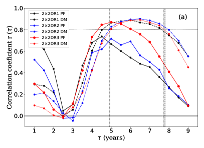
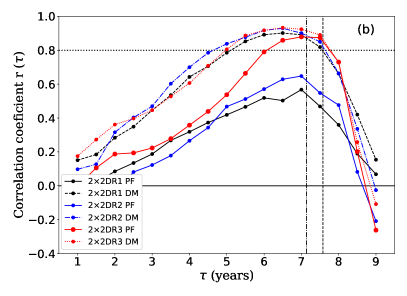
Figure 6.— Same as Fig. 4, for the 2$\times$2D dynamo model.

Activity level $T$ in the model is characterized by the total monthly number of emerging BMRs. For the precursor $P$ the polar cap flux PF (surface flux polewards of latitude $70^{\circ}$) and the global dipole moment DM are considered. The time variation of the correlation between $P$ and $T$ is displayed in Figure 6.

It is noteworthy that in the reference case (R1) only the global dipole moment performs truly well as a precursor. Reducing stochasticity, as in runs R2 and R3, improves the predictive skill of the polar fields, but the dipole moment still remains a better predictor, especially at early times. Correlations with the hemispherically averaged value of the polar field (not shown here) were found to follow a similar trend, so a difference in hemispherical coupling between the model and the real Sun does not explain the poorer performance of the polar fields with respect to the dipole moment. The better predictive skill of the dipole moment must then be related to the importance of fields at lower latitudes, possibly related to the overly dense concentration of the surface flux near the poles, due to the use of a high-latitude peaking latitudinal flow in the last optimized version of the 2$\times$2D model. This incoherence between the FTD and SFT optimizations was noticed in Lemerle & Charbonneau (2017) and still needs revisiting.

In the DM correlations, a short plateau is again seen in panel (a), indicating that the DM is a good precursor of the next cycle when evaluated 5 to 8 years before the next cycle maximum (roughly between DM peak and cycle minimum). This agrees well with observations, the extra year in temporal range attributable to the later peak amplitude (near symmetric cycle shape).

Similarly, in panel (b) the DM is found to be a good precursor of the next cycle amplitude 5 to 7 years following its reversal. It should be taken into account that the reversal in this model is more than a year earlier than observed; hence the cycle phase when acceptable predictions become possible is comparable to the observed range (which was acceptable for $\tau\gtrsim 4$ years after polar field reversal). Note also that the low correlations in the early years after DM reversal (panel (b)) are also coherent with observations. Before $\tau\approx 5$ years, not enough flux has reached the high latitudes to determine the faith of the next cycle, in the observed Sun and especially in this highly stochastic model.

As for the rising rate of polar fields with respect to the amplitude of the next cycle, results presented in the Appendix; Table 4 indicate that all models show some medium to high correlations, which are similar or higher than observations for the 2D and 3D models, but lower for the 2$\times$2D model. The correlations of the decay rate with amplitude presented in the Appendix; Table 5 show high values similar to observations for the polar fields (PF) of the 2D and 3D models, and for the dipole moment (DM) of the 2$\times$2D model.

4. Conclusions

We have presented an extensive performance analysis of various measures of the amplitude of the solar poloidal field as precursors of an upcoming solar cycle, based on both observational data and on the outputs of various existing flux transport dynamo models. We calculated correlation coefficients of the predictors with the next cycle amplitude as a function of time measured from several solar cycle landmarks. Setting a Pearson correlation level of $r=0.8$ as a lower limit for acceptable predictions, observations indicate that the earliest time when the polar predictor can be safely used is 4 years after polar field reversal. This is typically 2–3 years before solar minimum and about 7 years before the predicted maximum, considerably extending the temporal scope of the polar precursor method. Some correlation between the rise rate of the polar field with the next cycle amplitude gives an indication that the temporal scope of the precursor may be even longer in the Sun. From the observational record, the polar magnetic field, $A(t)$ index and global dipole moment are found to perform roughly equally well.

As the statistical sample upon which these conclusions are based is limited to a few well observed solar cycles, for further support of these findings we turned to dynamo models calibrated to realistically represent the observed solar cycle. The three models considered differ greatly in terms of their physical background and in the parameter regime in which they operate. They all involve significant simplifications and, unfortunately, all show obvious offsets in their relative phases and timings of characteristic solar cycle landmarks.

Nevertheless, all three models being self-consistent Babcock–Leighton type, they do produce the strong correlations expected between the poloidal field of an ongoing cycle and the following cycle amplitude. The stronger the correlations, the more deterministic is the model. In this sense, the Surya model allows for very early predictions, meaning that the stochastic emergence process plays only little role in the late phases of the cycle; at the other end the highly stochastic 2$\times$2D model is much more restrictive on its predictive window. The real Sun likely lies somewhere in that interval. Thus, where all the models agree, there is a good indicator of some robust feature. Our analysis of the precursor value and temporal range of polar cap flux and dipole moment in the models has shown that our main conclusion regarding the possibility of using the polar field or the dipole moment as a precursor 4 years after polar reversal holds in all of them. This supports the robustness of our main observational finding.

The temporal sequence and intervals between cycle landmarks are known to correlate with the cycle amplitude (the Waldmeier effect being an obvious example). This raises the possibility that for cycles stronger or weaker than average the time horizon $\tau$ for which reliable prediction are possible at $t=t_{p,rev}+\tau$ may show a systematic deviation from the typical value of 4 years deduced here. This issue could in principle be addressed by splitting the sample of cycles into subsamples according to strength and looking for systematic differences. The shortness of the observational data set, however, does not allow statistically meaningful inferences from such small samples. In the case of models, sample size restrictions do not arise but, as discussed in Section 3 above, the temporal sequence and spacing of cycle landmarks in these models do not represent observed solar cycles faithfully enough to give credit to inferences regarding such finer points as a possible amplitude dependence of the prediction horizon. Thus, it is at present not possible to exclude the possibility of an amplitude dependence in the result.

To illustrate our main conclusion,

we use WSO polar field measurements in March 2017 (4 years after polar reversal in Cycle 24) to predict the amplitude of the upcoming Cycle 25. For this purpose, linear regressions between the smoothed WSO polar field and peak sunspot area are used. Using hemispherically separated data we arrive at a prediction of $399.45\pm 105.05$ (North) and $744.38\pm 137.31$ (South), while using $(B_{N}-B_{S})/2$ as a predictor the total peak sunspot area is predicted as $553.29\pm 166.63$. This translates to a peak sunspot “number” of $120\pm 25$, based on a linear regression ($\mathrm{SSN}=0.152\rm{SSA}+36.565$) between the sunspot number (Version 2) vs. sunspot area.

Cycle 25 is now officially considered by SILSO to have started in December 2019. Using the predictor values at this epoch, a similar linear regression analysis yields the following updated predictions for the hemispheric peak sunspot areas: $663.71\pm 91.62$ (North), $523.94\pm 82.27$ (South). Again based on $(B_{N}-B_{S})/2$ the total peak sunspot area is predicted as $589.11\pm 21.84$. (This translates to a peak sunspot “number” of $126\pm 3$). We note that in these regression analyses, we got only three complete cycles; the WSO data for Cycle 20 was not complete.

For the calculation of the prediction error, we have take the standard deviations in the slope and intercept of the linear regression based on Bayesian probabilistic approach using Python’s Pymc3 routine. We also note that the error in the latter prediction based on the minima of $(B_{N}-B_{S})/2$ is very small because all three data points lie almost on a straight line, however, this did not happen in the prediction based on $(B_{N}-B_{S})/2$ at 4 years after the reversal.

It is thus apparent that the prediction made 3 years earlier, that is 4 years after the polar reversal, already yields a good approximation to the final forecast. Solar cycle 25 is predicted to be similar to or only slightly stronger than the previous cycle.

RISE AND DECAY RATES OF THE POLAR FIELD AS CYCLE PRECURSORS

Following a reversal, the observed polar field tends to increase at a fast rate to reach a plateau lasting until the next solar minimum (cf. Fig. 3). This suggests that the level of this plateau, and hence the predictor value 4 years after reversal might be anticipated based on the rate of this initial rise (or even the rate of the decay of the opposite polarity polar field before the reversal). This might push the temporal scope of the polar precursor even further back in time. Indeed, Petrovay et al. (2018) found that the rate at which the “rush to the pole” feature in coronal green line supersynoptic maps tends to the poles may be used as a precursor for the time of the next cycle maximum. Prompted by these considerations, here we take a closer look at any possible correlations between the rise/decay rate of the polar field around reversal and the amplitude of the next solar maximum.

Table 2Pearson’s correlation coefficients ($r$) and the $p$ values computed between the rise rate of the polar field/proxies and the amplitude of the next cycle maximum: observations.

	Polar faculae			WSO polar field			A(t) Index		DM
Rise rate	$r$ ($p$)			$r$ ($p$)			$r$ ($p$)		$r$ ($p$)
computed from	North	South		North	South
$t_{{\rm rev}}+1$ to $t_{{\rm rev}}+2$	0.57 (0.08)	0.28 (0.44)		0.34 (0.78)	$-0.28$ (0.81)		0.18 (0.68)		0.57 (0.61)
$t_{{\rm rev}}+2$ to $t_{{\rm rev}}+3$	0.19 (0.61)	0.56 (0.09)		0.69 (0.51)	0.99 (0.08)		0.64 (0.04)		0.67 (0.53)
$t_{{\rm rev}+1}$ to $t_{{\rm rev}}+3$	0.47 (0.16)	0.42 (0.23)		0.95 (0.19)	0.01 (0.99)		0.67 (0.07)		0.63 (0.56)
$t_{{\rm rev}}$ to $t_{{\rm rev}}+3$	0.51 (0.13)	0.61 (0.06)		0.98 (0.11)	0.98 (0.14)		0.77 (0.02)		0.48 (0.68)

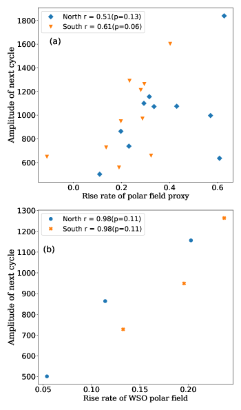
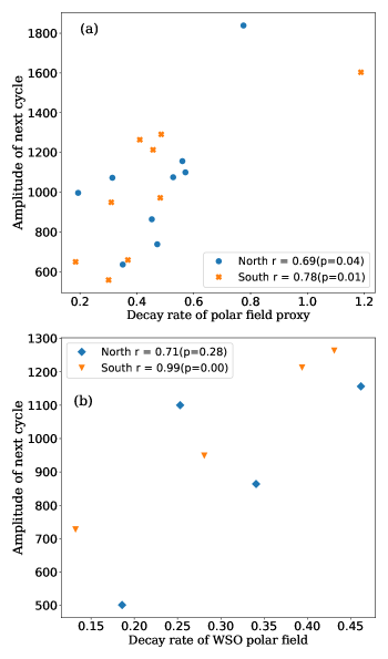
Figure 7.— Scatter plots between the rise rate (left) or decay rate (right) a predictor (top: MWO polar faculae count; bottom: WSO polar field) against the amplitude of the next cycle maximum. The rates are evaluated from the values taken at $t_{\rm rev}$ and $t_{\rm rev}+3$ (rise) and $t_{{\rm rev}-2}$ and $t_{{\rm rev}-1}$ (decay).

First we consider the rise rate. The rate can be computed in different ways and at different times in the rising phase of the polar field. We consider two points at a separation of $\Delta T$ and define the rate as the difference between the polar fields at these two points devided by $\Delta T$. This is illustrated in Figure 3. As the bin size of the polar field proxy data is one year, we cannot take $\Delta T$ less than one year. Table 2 shows correlation coefficients for the rise rates computed at different times. For two particular choices of the predictor and the time interval the corresponding scatter plot is shown in Figure 7 (left). The correlations are generally unconvincing, although the very limited number of data points for WSO measurements does occasionally result in Pearson correlation values close to one there.

Turning now to the decay rate, it is to be noted that the starting and end points of the base interval usually fall in the rise phase of the ongoing cycle. Hence, “next cycle maximum” in this case refers to the maximum of the ongoing cycle which is indeed found to be well predicted by the decay rate. This is shown in Figure 7 (right), with the correlation coefficients collected in Table 3. This correlation, however, is but a natural consequence of the fact that in a stronger cycle high rates of flux emergence are seen already in the rise phase, and the poleward transport of this new flux induces a more rapid decay of the polar fields left from the previous cycle. This result has little practical importance as the correlation values are generally no better than those of the conventional polar precursor method and the temporal scope is shorter.

Table 3Pearson’s correlation coefficients ($r$) and the $p$ values computed between the decay rate of the polar field/proxies and the amplitude of the next cycle maximum: observations.

	Polar faculae			WSO polar field			A$(t)$ Index		DM
Decay rate	$r$ ($p$)			$r$ ($p$)			$r$ ($p$)		$r$ ($p$)
computed from	North	South		North	South
$t_{{\rm rev}}-2$ to $t_{{\rm rev}}-1$	0.69 (0.04)	0.78 (0.01)		0.71 (0.28)	0.99 (0.00)		0.39 (0.37)		0.75 (0.24)
$t_{{\rm rev}}-3$ to $t_{{\rm rev}}-2$	0.66 (0.05)	0.67 (0.05)		0.10 (0.89)	0.54 (0.45)		0.63 (0.13)		0.58 (0.42)
$t_{{\rm rev}}-4$ to $t_{{\rm rev}}-3$	0.29 (0.45)	$-0.04$ (0.90)		$-0.91$ (0.26)	$-0.02$ (0.98)		0.89 (0.01)		0.58 (0.42)
$t_{{\rm rev}}-3$ to $t_{{\rm rev}}-1$	0.73 (0.02)	0.85 (0.01)		0.62 (0.37)	0.83 (0.16)		0.69 (0.16)		0.66 (0.33)
$t_{{\rm rev}}-4$ to $t_{{\rm rev}}-2$	0.47 (0.20)	0.32 (0.40)		$-0.43$ (0.71)	0.99 (0.01)		0.94 (0.01)		0.58 (0.42)
$t_{{\rm rev}}-4$ to $t_{{\rm rev}}-1$	0.60 (0.08)	0.82 (0.01)		0.94 (0.21)	0.99 (0.03)		0.84 (0.02)		0.63 (0.36)

Table 4Pearson’s correlation coefficients ($r$) and the $p$ values computed between the rise rate of the polar field/proxies and the amplitude of the next cycle maximum: models

	2DR1			2DR2			2DR3			3DR1			3DR2			3DR3			2$\times$2D-R1
Rise rate	$r$ ($p$)			$r$ ($p$)			$r$ ($p$)			$r$ ($p$)			$r$ ($p$)			$r$ ($p$)			$r$ ($p$)
computed from	PF	DM		PF	DM		PF	DM		PF	DM		PF	DM		PF	DM		PF	DM
$t_{{\rm rev}}+1$ to $t_{{\rm rev}}+2$	0.74	0.61		0.83	0.93		0.15	0.13		0.76	0.69		0.60	0.43		0.54	0.50		0.11	0.26
$t_{{\rm rev}}+2$ to $t_{{\rm rev}}+3$	0.57	0.27		0.66	0.79		0.18	0.16		0.78	0.57		0.59	0.40		0.60	0.49		0.11	0.28
$t_{{\rm rev}}+1$ to $t_{{\rm rev}}+3$	0.84	0.69		0.91	0.96		0.24	0.28		0.79	0.72		0.63	0.53		0.61	0.62		0.23	0.41
$t_{{\rm rev}}+1$ to $t_{{\rm rev}}+4$	0.87	0.70		0.89	0.96		0.37	0.37		0.88	0.75		0.72	0.59		0.74	0.60		0.35	0.58

For completeness, the corresponding results for the dynamo models are presented in Tables 4 and 5. These results are in agreement with the observational findings discussed above.

Table 5Pearson’s correlation coefficients ($r$) and the $p$ values computed between the decay rate of the polar field/proxies and the amplitude of the next cycle maximum: models

	2DR1			2DR2			2DR3			3DR1			3DR2			3DR3			2$\times$2D-R1
Decay rate	$r$ ($p$)			$r$ ($p$)			$r$ ($p$)			$r$ ($p$)			$r$ ($p$)			$r$ ($p$)			$r$ ($p$)
computed from	PF	DM		PF	DM		PF	DM		PF	DM		PF	DM		PF	DM		PF	DM
$t_{{\rm rev}}-2$ to $t_{{\rm rev}}-1$	0.88	0.89		0.83	0.98		0.30	0.64		0.83	0.30		0.60	0.46		0.74	0.37		0.52	0.83
$t_{{\rm rev}}-3$ to $t_{{\rm rev}}-2$	0.81	0.65		0.67	0.91		0.31	0.58		0.90	0.46		0.72	0.42		0.81	0.37		0.03	0.48
$t_{{\rm rev}}-4$ to $t_{{\rm rev}}-3$	0.41	0.02		0.24	0.68		0.35	0.49		0.91	0.57		0.80	0.34		0.70	0.41		0.00	$-0.03$
$t_{{\rm rev}}-3$ to $t_{{\rm rev}}-1$	0.91	0.89		0.89	0.98		0.34	0.64		0.91	0.47		0.72	0.45		0.82	0.42		0.32	0.79
$t_{{\rm rev}}-4$ to $t_{{\rm rev}}-2$	0.78	0.48		0.57	0.89		0.42	0.68		0.94	0.59		0.81	0.41		0.81	0.46		$-0.04$	0.28
$t_{{\rm rev}}-4$ to $t_{{\rm rev}}-1$	0.91	0.86		0.89	0.97		0.42	0.71		0.95	0.65		0.86	0.46		0.78	0.42		0.13	0.68

References

- Bhowmik & Nandy (2018) Bhowmik, P., & Nandy, D. 2018, Nature Communications, 9, 5209
- Cameron & Schüssler (2017) Cameron, R. H., & Schüssler, M. 2017, ApJ, 843, 111
- Charbonneau (2010) Charbonneau, P. 2010, Living Rev. Sol. Phys., 7, 3
- Charbonneau & Dikpati (2000) Charbonneau, P., & Dikpati, M. 2000, ApJ, 543, 1027
- Chatterjee et al. (2004) Chatterjee, P., Nandy, D., & Choudhuri, A. R. 2004, A&A, 427, 1019
- Choudhuri et al. (2007) Choudhuri, A. R., Chatterjee, P., & Jiang, J. 2007, Physical Review Letters, 98, 131103
- Dikpati & Charbonneau (1999) Dikpati, M., & Charbonneau, P. 1999, ApJ, 518, 508
- Hathaway (2015) Hathaway, D. H. 2015, Living Reviews in Solar Physics, 12, 4
- Hathaway et al. (2002) Hathaway, D. H., Wilson, R. M., & Reichmann, E. J. 2002, Sol. Phys., 211, 357
- Hazra et al. (2015) Hazra, G., Karak, B. B., Banerjee, D., & Choudhuri, A. R. 2015, Sol. Phys., 290, 1851
- Iijima et al. (2017) Iijima, H., Hotta, H., Imada, S., Kusano, K., & Shiota, D. 2017, A&A, 607, L2
- Jha et al. (2020) Jha, B. K., Karak, B. B., Mandal, S., & Banerjee, D. 2020, ApJ, 889, L19
- Jiang (2020) Jiang, J. 2020, ApJ in press, arXiv: 2007.07069
- Jiang et al. (2007) Jiang, J., Chatterjee, P., & Choudhuri, A. R. 2007, MNRAS, 381, 1527
- Jiang et al. (2018) Jiang, J., Wang, J.-X., Jiao, Q.-R., & Cao, J.-B. 2018, The Astrophysical Journal, 863, 159
- Karak (2010) Karak, B. B. 2010, ApJ, 724, 1021
- Karak (2020) —. 2020, arXiv e-prints, arXiv:2009.06969
- Karak & Choudhuri (2011) Karak, B. B., & Choudhuri, A. R. 2011, MNRAS, 410, 1503
- Karak et al. (2018) Karak, B. B., Mandal, S., & Banerjee, D. 2018, ApJ, 866, 17
- Karak & Miesch (2017) Karak, B. B., & Miesch, M. 2017, ApJ, 847, 69
- Kitchatinov et al. (2018) Kitchatinov, L. L., Mordvinov, A. V., & Nepomnyashchikh, A. A. 2018, A&A, 615, A38
- Kitchatinov & Olemskoy (2011) Kitchatinov, L. L., & Olemskoy, S. V. 2011, Astronomy Letters, 37, 656
- Labonville et al. (2019) Labonville, F., Charbonneau, P., & Lemerle, A. 2019, Sol. Phys., 294, 82
- Lemerle & Charbonneau (2017) Lemerle, A., & Charbonneau, P. 2017, ApJ, 834, 133
- Lemerle et al. (2015) Lemerle, A., Charbonneau, P., & Carignan-Dugas, A. 2015, ApJ, 810, 78
- Makarov et al. (1989) Makarov, V. I., Makarova, V. V., & Sivaraman, K. R. 1989, Sol. Phys., 119, 45
- Makarov et al. (2001) Makarov, V. I., Tlatov, A. G., Callebaut, D. K., Obridko, V. N., & Shelting, B. D. 2001, Sol. Phys., 198, 409
- Miesch & Dikpati (2014) Miesch, M. S., & Dikpati, M. 2014, ApJ, 785, L8
- Miesch & Teweldebirhan (2016) Miesch, M. S., & Teweldebirhan, K. 2016, Space Sci. Rev.
- Muñoz-Jaramillo et al. (2013) Muñoz-Jaramillo, A., Dasi-Espuig, M., Balmaceda, L. A., & DeLuca, E. E. 2013, ApJ, 767, L25
- Muñoz-Jaramillo et al. (2012) Muñoz-Jaramillo, A., Sheeley, N. R., Zhang, J., & DeLuca, E. E. 2012, ApJ, 753, 146
- Nagy et al. (2017) Nagy, M., Lemerle, A., Labonville, F., Petrovay, K., & Charbonneau, P. 2017, Sol. Phys., 292, 167
- Pesnell (2012) Pesnell, W. D. 2012, Sol. Phys., 281, 507
- Petrovay (2020) Petrovay, K. 2020, Living Reviews in Solar Physics, 17, 2
- Petrovay et al. (2018) Petrovay, K., Nagy, M., Gerják, T., & Juhász, L. 2018, J. Atmos. Sol.-Terr. Phys., 176, 15
- Petrovay & Talafha (2019) Petrovay, K., & Talafha, M. 2019, A&A, 632, A87
- Priyal et al. (2014) Priyal, M., Banerjee, D., Karak, B. B., Muñoz-Jaramillo, A., Ravindra, B., Choudhuri, A. R., & Singh, J. 2014, ApJ, 793, L4
- Schatten et al. (1978) Schatten, K. H., Scherrer, P. H., Svalgaard, L., & Wilcox, J. M. 1978, Geophys. Res. Lett., 5, 411
- Sheeley (1991) Sheeley, N. R., J. 1991, ApJ, 374, 386
- Upton & Hathaway (2018) Upton, L. A., & Hathaway, D. H. 2018, Geophys. Res. Lett., 45, 8091
- Wang & Sheeley (2009) Wang, Y.-M., & Sheeley, N. R. 2009, ApJ, 694, L11
- Wang & Sheeley (1989) Wang, Y.-M., & Sheeley, Jr., N. R. 1989, Sol. Phys., 124, 81
- Yeates & Muñoz-Jaramillo (2013) Yeates, A. R., & Muñoz-Jaramillo, A. 2013, MNRAS, 436, 3366