Computer Architecture-Aware Optimisation of DNA Analysis Systems School of Computer Science and Engineering Hasindu Gamaarachchi z5136909 Doctor of Philosophy November 2020 Sri Parameswaran

Abstract

DNA sequencing—the process that converts the massive amount of chemically encoded data in DNA molecules into a computer-readable form—is revolutionising the field of medicine through a variety of applications such as precision medicine, accurate diagnostics and identifying disease predisposition. DNA sequencing also has many other applications in areas such as epidemiology, forensics and evolutionary biology. DNA sequencers, the machines which perform DNA sequencing, have evolved from the size of a fridge to that of a mobile phone over the last two decades. The cost of sequencing a complete human genome has remarkably reduced from billions of dollars to hundreds of dollars over this time. The size of a DNA sequencer is expected to become even smaller and the sequencing cost per genome is expected to be even more affordable in the future. Thus, DNA tests are likely to be performed as routinely and cost-effectively as today’s blood tests. Despite the reduction in size and cost, DNA sequencers output hundreds or thousands of gigabytes of necessary data to account for errors made during the sequencing process. This data must be analysed on computers to discover meaningful information (for instance, mutations and epigenetic modifications) that have biological implications. Unfortunately, the analysis techniques have not kept the pace with rapidly improving sequencing technologies. Consequently, even today, the process of DNA analysis is performed on high-performance computers, just as it was a couple of decades ago. Such high-performance computers are not portable, unlike mobile phone-sized ultra-portable sequencers. Consequently, the full utility of an ultra-portable sequencer for sequencing in-the-field or at the point-of-care is limited by the lack of portable lightweight analytic techniques.

A primary reason for this lag between the two technologies is because sequence analysis software tools written by computational biologists with the focus on higher accuracy of the results are un-optimised to efficiently utilise computational resources (i.e. software does not map well to the architecture of computers). This thesis proposes computer architecture-aware optimisation of DNA analysis software. DNA analysis software is inevitably convoluted due to the complexity associated with biological data. Modern computer architectures are also complex. Performing architecture-aware optimisations requires the synergistic use of knowledge from both domains, (i.e, DNA sequence analysis and computer architecture). Computer architecture knowledge helps the efficient mapping and exploitation of existing hardware resources, while the understanding of DNA sequence analysis ensures that the final accuracy of the results is intact. In a nutshell, this thesis aims to draw the two domains together.

In this thesis, gold-standard DNA sequence analysis workflows (a workflow is a few software tools executed sequentially where each software tool is a complex system of dozens of algorithms) are systematically examined for algorithmic components that cause performance bottlenecks. Identified bottlenecks are resolved through architecture-aware optimisations at different levels, i.e., memory level, cache level, register level and processor level. Some example optimisations are: 1, the cache-friendly optimisation of de Bruijn graph construction that is a time-consuming core-component in a branch of software tools called variant callers (2X performance improvement); 2, memory capacity optimisation of reference indexes for the process called read alignment (from 16GB up to 2GB); 3, memory and processor level optimisation (for CPU-GPU heterogeneous systems) of an important time-consuming algorithm called adaptive banded event alignment used for the latest nanopore sequencing technology (3-5X performance improvement). Instead of merely performing algorithmic optimisations, those optimised versions are integrated back to the software and it is demonstrated that there is global efficiency and the accuracy is unaffected. Finally, the optimised software tools are used in complete end-to-end analysis workflows and their efficacy is demonstrated by running on prototypical embedded systems. The embedded systems are not only fully functional, but the performance is also comparable to an unoptimised workflow on a high-performance computer. The practicality of these embedded systems has been demonstrated by integrating into the sequencing facility at the Garvan Institute of Medical Research in Sydney. Such low cost, energy-efficient, sufficiently fast and portable embedded systems enable complete DNA analysis at the point-of-care or in-the-field. Work conducted under this thesis also contributes to the bioinformatics community through contributions to popular bioinformatics tools (i.e. Platypus, Minimap2 and Nanopolish) and the design and development of novel open-source bioinformatics software (f5c).

Publications and Presentations

List of Publications

This thesis has led to the following first author journal publications and they are included in lieu of chapters.

• H. Gamaarachchi, A. Bayat, B. Gaeta, and S. Parameswaran, “Cache Friendly Optimisation of de Bruijn Graph based Local Re-assembly in Variant Calling,” IEEE/ACM transactions on computational biology and bioinformatics, 2018. DOI: https://doi.org/10.1109/TCBB.2018.2881975

• H. Gamaarachchi, S. Parameswaran, and M. A. Smith, “Featherweight long read alignment using partitioned reference indexes,” Scientific Reports 9, 4318 (2019). DOI: https://doi.org/10.1038/s41598-019-40739-8

• H. Gamaarachchi, C. W. Lam, G. Jayatilaka, H. Samarakoon, J. T. Simpson, M. A. Smith, and S. Parameswaran, “GPU Accelerated Adaptive Banded Event Alignment for Rapid Comparative Nanopore Signal Analysis,” BMC Bioinformatics 21, 343 (2020). DOI: https://doi.org/10.1186/s12859-020-03697-x, 2020.

• H. Gamaarachchi, H. Saadat, S. Parameswaran, "Optimisation of Nanopore Sequence Analysis Software for Many-core CPUs", prepared for submission [in progress], 2020.

This thesis has also led to the following article in the ACM SRC Grand Finals.

• “ESWEEK: G: Real-time, Portable and Lightweight Nanopore DNA Sequence Analysis using System-on-Chip”, ACM SRC Grand Finals, 2020. URL: https://src.acm.org/binaries/content/assets/src/2020/hasindu-gamaarachchi.pdf — third place Grand Finalist

Collaborative research conducted in close relation to the work presented under this thesis has led to the following publications and pre-prints which are not included in the thesis.

• H. Samarakoon, S. Punchihewa, A. Senanayake, J. M. Hammond, I. Stevanovski, J.M. Ferguson, R. Ragel, H. Gamaarachchi and I. W. Deveson, “Genopo: a nanopore sequencing analysis toolkit for portable Android devices,” Communications biology 3, 538 (2020) DOI: https://doi.org/10.1038/s42003-020-01270-z

• R. P. Mohanty, H. Gamaarachchi, A. Lambert, and S. Parameswaran, “SWARAM: Portable Energy and Cost Efficient Embedded System for Genomic Processing,” ACM Transactions on Embedded Computing Systems (TECS) 18.5s (2019). DOI: https://doi.org/10.1145/3358211

• A. Bayat, H. Gamaarachchi, N. P. Deshpande, M. R. Wilkins, and S. Parameswaran, “Methods for de-novo genome assembly,” Preprints 2020, 2020, DOI: https://doi.org/10.20944/preprints202006.0324.v1

• A.F. Laguna, H. Gamaarachchi, X. Yin, M.Niemier, S. Parameswaran and X. S. Hu, “Seed-and-Vote based In-Memory Accelerator for DNA Read Mapping”, ICCAD 2020 [accepted]

List of Presentations

Oral presentations:

• "Performance Optimisation of Nanopore DNA Analysis Software: A Computer Architecture Aware Approach," Australasian Leadership Computing Symposium (ALCS), 2019. URL: https://opus.nci.org.au/display/Help/Genomics+Stream?preview=/48497246/50236166/ALCS_Genomics_Gamaarachchi_released.pdf

• "Lightweight, Portable and Real-time Embedded Computing Systems for Downstream Nanopore Data Processing", London Calling, 2020. URL: https://www.youtube.com/watch?v=hvXSpqnIB1c

• "Real-time, Portable and Lightweight Nanopore DNA Sequence Analysis using System-on-Chip", ACM SRC second-round at ESWEEK, 2019. — First place and entry into the SRC Grand Finals

Poster presentations:

• "Portable Real-time Genomic Data Processing: Harmonising Bioinformatics Software to Exploit Hardware", Australasian Genomic Technologies Association Conference (AGTA) 2019. — Best student poster award

• "Real-time, Portable and Lightweight Nanopore DNA Sequence Analysis using System-on-Chip", ACM SRC first-round at ESWEEK, 2019. — Entry into the second-round

Awards

The work conducted under this thesis has received the following awards.

• Grand Finalist (third place winner), ACM SRC Grand Finals graduate category, 2020

• First Place, ACM SIGBED SRC at ESWEEK, 2019

• Best Student Poster Award, Australasian Genomic Technologies Association Conference (AGTA), 2019

• Runner-up, UNSW 3 Minute Thesis School level, 2019

Contents

1. Abstract
2. Acknowledgement
3. Publications and Presentations
4. Awards
5. 1 Introduction
   1. 1.1 Sequencers vs Computers - Gap Between Technologies
   2. 1.2 Need for Reducing the Gap
   3. 1.3 Possible Solutions to Fill the Gap
   4. 1.4 This Thesis
      1. 1.4.1 Philosophy
      2. 1.4.2 Chapter Outline
      3. 1.4.3 Publications
      4. 1.4.4 Open-source Contributions
      5. 1.4.5 Miscellaneous
6. 2 Literature Review
   1. 2.1 DNA Sequencing
      1. 2.1.1 Terminology and Basics of DNA
      2. 2.1.2 DNA Sequencing Technologies
   2. 2.2 Sequence Analysis
      1. 2.2.1 Reference-guided second-generation workflow
      2. 2.2.2 Reference-guided third-generation workflow for nanopore data
      3. 2.2.3 De novo assembly
   3. 2.3 Related Work
      1. 2.3.1 CPU/HPC/Cloud
      2. 2.3.2 Graphics Processing Units (GPU)
      3. 2.3.3 Field Programmable Gate Arrays (FPGA)
      4. 2.3.4 Application-specific Hardware
7. 3 Cache Friendly Variant Calling
   1. 3.1 Introduction
   2. 3.2 Background of deBruijn Graph based Local Re-assembly
   3. 3.3 Baseline Algorithm
   4. 3.4 Methodology
      1. 3.4.1 Simplified Overview
      2. 3.4.2 Algorithm in Depth
   5. 3.5 Results
   6. 3.6 Discussion
   7. 3.7 Summary
8. 4 Featherweight Long Read Alignment
   1. 4.1 Introduction
   2. 4.2 Results
      1. 4.2.1 Effect of parameters on memory usage
      2. 4.2.2 Caveats of naive partitioned indexes
      3. 4.2.3 Effect of using a partitioned index on alignment accuracy
      4. 4.2.4 Memory usage and runtime of partitioned indexes
   3. 4.3 Discussion
   4. 4.4 Materials and methods
      1. 4.4.1 Exploration of parameters that affect memory usage in Minimap2
      2. 4.4.2 Merging of mappings from a partitioned Index
      3. 4.4.3 Chromosome balancing
      4. 4.4.4 Datasets and evaluation methodology
   5. 4.5 Summary
   6. 4.6 Data Availability
9. 5 GPU Accelerated Adaptive Banded Event Alignment
   1. 5.1 Introduction
   2. 5.2 Background
      1. 5.2.1 Nanopore sequencing and analysis
      2. 5.2.2 Methylation calling
      3. 5.2.3 Adaptive Banded Event Alignment (ABEA)
      4. 5.2.4 GPU architecture and programming
   3. 5.3 Related work
   4. 5.4 Methodology
      1. 5.4.1 Parallelisation and compute optimisations
      2. 5.4.2 Memory optimisation
      3. 5.4.3 Heterogeneous processing
   5. 5.5 Results
      1. 5.5.1 Experimental setup
      2. 5.5.2 Effect of individual optimisations
      3. 5.5.3 Speedup of Adaptive Banded Event Alignment
      4. 5.5.4 Total run-time of f5c compared with original Nanopolish
   6. 5.6 Discussion
   7. 5.7 Summary
10. 6 System Integration
    1. 6.1 Introduction
    2. 6.2 System Architecture of Nanopore-cluster
       1. 6.2.1 Hardware Architecture
       2. 6.2.2 Software Architecture
    3. 6.3 Experimental Setup
       1. 6.3.1 Rock64-cluster Hardware Setup
       2. 6.3.2 Rock64-cluster Software Setup
       3. 6.3.3 NVIDIA Jetson SBCs
       4. 6.3.4 Datasets
    4. 6.4 Results
       1. 6.4.1 Rock64-cluster
       2. 6.4.2 On NVIDIA Jetson SBCs
       3. 6.4.3 Real-time Processing Capability
       4. 6.4.4 Comparison with HPC
    5. 6.5 Discussion
       1. 6.5.1 Implementation for On-the-fly Processing
       2. 6.5.2 Mobile Phone Cluster
       3. 6.5.3 Potential Diagnostic Applications
    6. 6.6 Summary
11. 7 I/O Optimisations
    1. 7.1 Introduction
    2. 7.2 Background
       1. 7.2.1 I/O
       2. 7.2.2 Nanopore raw data analysis
    3. 7.3 Identification and Explanation of bottleneck
       1. 7.3.1 Identification of the Bottleneck
       2. 7.3.2 Verification of the Identified Bottleneck
       3. 7.3.3 Detailed Explanation of the Identified Bottleneck
    4. 7.4 Proposed Optimisations
       1. 7.4.1 Alternate File Format (SLOW5)
       2. 7.4.2 Multi-process based Solution
       3. 7.4.3 Restructuring & Miscellaneous Optimisations
    5. 7.5 Experiment and Results
       1. 7.5.1 Experimental Setup
       2. 7.5.2 Results: Alternate File Format (SLOW5)
       3. 7.5.3 Results: Multi-process Pool
       4. 7.5.4 Comparison of SLOW5 to FAST5 with Multi-process Pool
       5. 7.5.5 Comparison with Multi-FAST5 Format
       6. 7.5.6 On NFS
    6. 7.6 Discussion
       1. 7.6.1 Other Possible Solutions
       2. 7.6.2 Future Directions
       3. 7.6.3 Potential Impact on other Toolkits and Domains
    7. 7.7 Summary
12. 8 Conclusion and Future Directions
    1. 8.1 Future Directions
13. A Appendix: Featherweight Long Read Alignment
    1. A.1 Supplementary Note 1
       1. A.1.1 Serialising (dumping) of the internal state
       2. A.1.2 Merging operation
       3. A.1.3 Emulated single reference index
    2. A.2 Chromosome Balancing
       1. A.2.1 Memory efficiency for references with unbalanced lengths
    3. A.3 Supplementary Note 3 - Instructions to run the tools
       1. A.3.1 Example
       2. A.3.2 Index construction with chromosome size balancing
       3. A.3.3 Running Minimap2 on a partitioned index with merging
14. B Appendix: f5c Documentation
    1. B.1 Readme
       1. B.1.1 Quick start
       2. B.1.2 Building
       3. B.1.3 Usage
       4. B.1.4 Acknowledgement
    2. B.2 Building f5c
       1. B.2.1 Method 1 (recommended)
       2. B.2.2 Method 2 (time consuming)
       3. B.2.3 Method 3 (not recommended)
       4. B.2.4 Docker Image
       5. B.2.5 CUDA Troubleshooting
       6. B.2.6 Compiling Issues
       7. B.2.7 Runtime Errors
       8. B.2.8 Commands and options
       9. B.2.9 Available f5c tools
15. C Appendix: f5c
    1. C.1 Why Nanopolish had to be re-engineered?
    2. C.2 Additional advantages of f5c over Nanopolish
16. D Appendix: Portable Binaries
    1. D.1 Key points
    2. D.2 A case study with f5c
       1. D.2.1 Note on CUDA libraries
       2. D.2.2 Example commands
17. E Appendix: Rock64-cluster and f5p
    1. E.1 Rock64-cluster
       1. E.1.1 Required Hardware
       2. E.1.2 Connecting nodes together
       3. E.1.3 Setting up the head node
       4. E.1.4 Compiling software and preparing the folder structure
       5. E.1.5 Setting up woker nodes
    2. E.2 f5p
       1. E.2.1 Pre-requisites
       2. E.2.2 Getting started
       3. E.2.3 Building and initial configuration
       4. E.2.4 Running for a dataset
18. F Appendix: Bioinformatics on Mobile Phone
    1. F.1 Requirements
    2. F.2 Steps
    3. F.3 Examples
       1. F.3.1 minimap2
       2. F.3.2 Samtools
       3. F.3.3 F5C
       4. F.3.4 Nanopolish
    4. F.4 Running Directly on Phone
       1. F.4.1 On Android 7.0 or before
       2. F.4.2 On Android 8.x
       3. F.4.3 Is there a proper way?
19. G Appendix: Open-source Contributions
    1. G.0.1 User comments for f5c
    2. G.0.2 Contributions to Minimap2
    3. G.0.3 Contributions to Nanopolish
20. H Appendix: I/O Optimisations
    1. H.1 Extended Motivational Example on another System
    2. H.2 Extended Bottleneck using Another Dataset
    3. H.3 Extended Results
       1. H.3.1 Results from Alternate File Format (SLOW5) for Another Dataset
       2. H.3.2 Impact of Proposed Solutions on Disk IOPS
21. I Appendix: Poster Presentations

List of Figures

1. 1.1 DNA sequencing and sequence analysis
2. 1.2 Human DNA sequence printed as a series of books
3. 1.3 Drop of DNA sequencing cost per human genome over the period from 2001 to 2019
4. 1.4 Evolution of sequencing machines
5. 1.5 Synergistic use of knowledge from both computer architecture and biology
6. 2.1 The DNA molecule and a chromosome
7. 2.2 An example of FASTA file format
8. 2.3 Elaboration of SNV and Indels
9. 2.4 An example of VCF file format
10. 2.5 Elaboration of the concept of coverage in sequencing.
11. 2.6 An example of FASTQ file format
12. 2.7 First-generation sequencers
13. 2.8 Illumina second-generation sequencers
14. 2.9 Pacific Biosciences Sequel Sequencer.
15. 2.10 Nanopore third-generation sequencers
16. 2.11 ONT MinIT, PromethION compute tower and MinION Mk1C
17. (a) MinION sequencer (right) connected to the MinIT base-calling unit (left)
18. (b) PromethION sequencer (left) and its compute tower (right)
19. (c) MinION Mk1C sequencer with integrated base-calling unit
20. 2.12 Simplified second-generation workflow
21. 2.13 GATK Best Practices pipeline.
22. 2.14 Simplified illustration of aligned sequence reads to a reference
23. 2.15 Dynamic programming based sequence alignment
24. (a) optimal sequence alignment
25. (b) Banded sequence alignment (band-width=4)
26. 2.16 Simplified elaboration of variant calling
27. 2.17 A screenshot from IGV from an NA12878 dataset
28. 2.18 Simplified third-generation nanopore workflow
29. 2.19 Evolution of dynamic programming-based sequence alignment
30. (a) Banded sequence alignment (band-width=3)
31. (b) Adaptive banded sequence alignment
32. 2.20 Read length distribution nanopore consortium
33. 2.21 A screenshot from IGV from an NA12878 nanopore dataset
34. 3.1 Distribution of execution time for Platypus variant caller
35. 3.2 A region of the reference and few mapped reads
36. 3.3 De Bruijn graph for the region
37. 3.4 The hash table
38. 3.5 Elaboration of how mapping information is used for improving cache performance
39. 3.6 Summary of the outcome of the proposed method
40. 3.7 Distribution of memory accesses in the optimised implementation
41. 3.8 Execution time for the baseline implementation and the modified implementation
42. 4.1 Effect of parameters on memory usage, performance and accuracy
43. 4.2 Effect of the window size parameter on the MAPQ distribution for synthetic spike-in controls
44. 4.3 Effect of aligning sequences to single vs partitioned indexes
45. 4.4 Effect of using partitioned indexes versus a single reference index on alignment quality
46. 4.5 Features of alignments that were discordantly mapped in single-idx and 16-part-idx-merged indexing strategies
47. 4.6 Genome browser screenshots of alignments unique to the 16-part-idx-merged that do not overlap annotated repeats
48. 4.7 Distribution of MAPQ and DP alignment score for the disparate mappings (different by at least one base position) between single-idx and 16-part-idx-merged
49. 4.8 Scatter plot of alignment scores of single-idx vs 16-part-idx-merged for disparate alignments (different by at least one base position)
50. 4.9 Distribution of genomic features of disparate alignments (different by at least one base position) between single-idx and 16-part-idx-merged
51. 4.10 Statistics and genomic features of disparate mappings (mapping positions not overlapping at least by 10%) between single-idx and 16-part-idx-merged
52. 4.11 Alignment of an ultra-long Nanopore read from a chromothriptic region
53. 4.12 Peak memory usage and runtime for a partitioned index of the GRCh38 human reference genome
54. 4.13 Effect of the window size on the error rate and sensitivity for simulated reads
55. 5.1 Nanopore portable sequencer and associated data analysis
56. 5.2 Illustration of a nanopore raw signal, events and pore-model
57. (a) An example nanopore raw signal and events
58. (b) an example pore-model
59. 5.3 example nanopore read length distributions
60. 5.4 Adaptive Banded Event Alignment
61. (a) band movement
62. (b) computing a single cell score
63. (c) trace-back
64. 5.5 Thread configuration of pre-kernel
65. 5.6 Thread assignment of pre-kernel
66. 5.7 Utility of kcache in the core-kernel to improve memory coalescing
67. (a) Random accesses to the model array (red arrows) when kcache is not employed
68. (b) Construction of the kcache in pre-kernel
69. (c) Spatially local memory accesses (green arrows) when kcache is employed
70. 5.8 Decision trees for resource optimisation
71. (a) memory balancing
72. (b) load balancing
73. 5.9 Effect of individual optimisations
74. (a) Distribution of GPU kernel execution time
75. (b) Time for GPU kernels compared cudaMalloc
76. (c) Effect of the read length on the speedup
77. (d) need for load-balancing based on read lengths
78. 5.10 Speedup of ABEA on GPU compared to CPU
79. (a) Performance comparison of ABEA on CPU vs GPU for D_small over a wide range of systems
80. (b) Performance comparison of ABEA on CPU vs GPU across full datasets
81. 5.11 Comparison of f5c to Nanopolish
82. 5.12 Human genome processing on-the-fly
83. 6.1 Hardware architecture of the proposed system
84. 6.2 Rock64-cluster placed alongside the nanopore sequencers at Garvan Institute of Medical Research
85. 6.3 Construction of the Rock64-cluster.
86. (a) A newly opened Rock64 SBC. Photograph credit: Martin A. Smith.
87. (b) Rock64 SBCs stacked using M2.5 cylinders. Photograph credits: Martin A. Smith.
88. (c) Rock64 SBCs connected using Ethernet
89. 6.4 Methylation calling workflow and its software tools
90. 6.5 Screenshot from Ganglia monitoring system
91. 6.6 Screenshot from LogAnalyzer
92. 6.7 NVIDIA Jetson development boards. Photograph credits: Hsu-Kang Dow.
93. (a) Jetson TX2 development board
94. (b) Jetson nano development board
95. 6.8 Comparison of Jetson TX2, Jetson Nano and Rock64 based on the single SBC execution times for the whole dataset
96. 6.9 Execution time on individual SBCs per each batch in the dataset
97. (a) On a single Rock64 development board
98. (b) On a single Jetson TX2 development board
99. (c) On a single Jetson nano development board
100. 6.10 The comparison of the sequencing rate with the data analysis rate over the duration of the sequencing run
101. 6.11 Comparison of proposed architecture on the Rock64-cluster with the original pipeline running on an HPC
102. 6.12 Methylation calling workflow on an Android mobile phone
103. 6.13 Potential applications of real-time methylation calling
104. 7.1 Variation of (a) execution time, (b) CPU utilisation and core-hours in original Nanopolish with the number of data processing threads.
105. (a) Execution time
106. (b) CPU utilisation & core-hours
107. 7.2 Elaboration of synchronous I/O
108. 7.3 Elaboration of multi threaded synchronous I/O
109. 7.4 Elaboration of asynchronous I/O
110. 7.5 Decomposition of time for individual components in restructured Nanopolish.
111. 7.6 Elaboration of the limitation in HDF library.
112. 7.7 The proposed multi-process based solution.
113. 7.8 Flow diagram depicting modifications to Nanopolish
114. 7.9 Overall execution time and CPU utilisation when SLOW5 format is used
115. (a) Execution time
116. (b) CPU utilisation
117. 7.10 Comparison of FAST5 vs SLOW5 access
118. (a) On system S1: HDD RAID
119. (b) On system S2: SSD RAID
120. 7.11 Overall results for multi-process pool
121. (a) Execution time
122. (b) CPU utilisation
123. 7.12 FAST5 file access using multiple I/O threads vs I/O processes
124. (a) On system S1: HDD RAID
125. (b) On system S2: SSD RAID
126. 7.13 Single-FAST5 vs Multi-FAST5 using I/O threads
127. (a) On system S1: HDD RAID
128. (b) On system S2: SSD RAID
129. 7.14 Single-FAST5 vs Multi-FAST5 using I/O processes
130. (a) On system S1: HDD RAID
131. (b) On system S2: SSD RAID
132. 7.15 Performance on NFS
133. (a) SLOW5 performance on NFS
134. (b) FAST5 performance on NFS
135. F.1 CPU and RAM usage
136. (a) CPU Usage
137. (b) RAM usage
138. F.2 Executing Minimap2 using terminal emulator
139. (a) Entering Commands
140. (b) Minimap2 execution
141. (c) SAM output
142. F.3 Remote ADB
143. F.4 Execution using remote ADB
144. H.1 Variation of runtime of original Nanopolish with the number of threads
145. H.2 CPU utilisation with the runtime
146. H.3 Inefficiency of multi-threaded I/O to the HDF5 library
147. (a) on system S1 comprising HDD RAID
148. (b) on system S2 comprising SSD RAID
149. H.4 Statistics collected using collectl for Nanopolish
150. H.5 Statistics collected using collectl for SLOW5
151. H.6 Statistics collected using collectl for FAST5 multi-process pool
152. I.1 Poster presented at AGTA 2019
153. I.2 Poster presented at ACM SRC at ESWEEK 2019

List of Tables

1. 2.1 Genome size of various organisms
2. 3.1 Memory access distribution in the optimised implementation
3. 4.1 Memory usage of Minimap2 for default parameters
4. 4.2 Statistics for alignment outputs for 689,781 reads from NA12878
5. 4.3 Mappings of the chromothriptic read which are different in single-idx and 16-part-idx-merged
6. 4.4 Detailed runtime for partitioned indexes
7. 5.1 Data arrays associated with ABEA and their sizes
8. 5.2 GPU data arrays, pointer computation and heuristically determined sizes
9. (a) Computation of pointer for the read i
10. (b) Heuristic allocation
11. 5.3 measured quantities
12. 5.4 adjustable user parameters
13. 5.5 Information of the datasets
14. 5.6 Different systems used for experiments
15. 6.1 Execution results of several nanopore datasets of the human genome on the Rock64-cluster
16. 7.1 Example of SLOW5 file format
17. 7.2 Example of SLOW5 index
18. 7.3 Dataset
19. 7.4 Computer systems
20. H.1 An Oxford Nanopore PromethION dataset
21. H.2 System used for experiment in section H.1

Chapter 1 Introduction

Humankind technologically advanced to read or ‘sequence’ their own DNA—nature’s blueprint of a living organism—only a few decades ago. This technological advancement was a turning point for healthcare and medicine and led to a new era of medicine that is more precise and tailored to an individual than traditional evidence-based medicine. Sequencing of the first-ever human DNA started as an international effort called the human genome project in 1990 and took 13 years to complete in 2003 [1], at a cost of 2.7 billion USD [2]. Since then, DNA sequencing technologies advanced at a remarkable pace over the last few decades up to a point where today the human genome can be sequenced in just two days at a cost less than 1000 USD [3]. This rapid pace of advancement is continuing, and this sequencing process is becoming possible within a few hours [4] at a cost of less than 100 USD [5]. Thus, DNA sequencing tests are likely to become routine as of today’s blood tests in the near future.

Precision medicine considers the variability in genes, environment and lifestyle amongst different individuals to guide the use of effective and safe treatments tailored to a particular individual [6]. This is in contrast to the one-size-fits-all approach in traditional evidence-based medicine that targets the average person [6]. Clinical genomics that considers the information encoded in the DNA is being increasingly incorporated into precision medicine protocols [7]. One of the ten highest-grossing drugs (in the USA), rosuvastin—a statin used to lower blood cholesterol—is shown to benefit only 1 in 20 [8]. The best benefit ratio for any of the top 10 grossing drugs is 1 in 4, which is still considerably low [8]. In traditional evidence-based medicine, selecting the most effective drug out of available subtypes of drugs for a particular patient is a somewhat trial-and-error process, which is inefficient [9]. In precision medicine, genetic information gathered from the sequencing of individuals’ DNA is being increasingly used to determine the most effective drug. For instance, the latest anti-cancer drugs such as crizotinib that treat anaplastic lymphoma kinase (ALK) positive lung cancer already require genetic testing of the patient [10]. While genetic testing today is mainly performed for critical cases, it is expected to become more and more frequent in the future with the cost and availability of DNA sequencing improving rapidly.

Another use of DNA sequencing is for implementing a more proactive approach, "prevention is better than cure". The genetic information of an individual can determine the predisposition to a number of diseases, thus making it possible to implement preventive measures. A very popular example is the actress Angelina Jolie who underwent a double mastectomy in 2013 after a genetic test that revealed a significantly higher chance of developing breast cancer. While the cost of a genetic test in 2013 was probably not affordable for everyone, today they are becoming more and more realistic and common.

DNA sequencing is also beneficial in epidemiological applications. In the recent past, during the Ebola virus outbreak in West Africa (2013–2016) and Zika virus outbreak in Brazil (2015-2016) DNA sequencing has been utilised for viral surveillance. Today, the utility of DNA sequencing is evident than ever before, due to the ongoing COVID-19 pandemic. DNA sequencing of the viral sequence allows identification of mutations that facilitates the tracking of the disease spread and provides insights into the virus evolution that are useful in vaccine development.

In addition to the above, DNA sequencing is also applicable in several other fields such as forensics, evolutionary biology and agronomy.

DNA sequencing alone is of limited utility if not for the sequence analysis, a very heavy computational analysis that follows the actual sequencing. DNA sequencers—the machines that sequence the DNA—read the DNA sequence in small fragments called ‘reads’. Computational analyses must be performed to put these reads together to achieve a draft sequence assembly close as possible to the original DNA sequence or to compare against an existing reference of the original DNA sequence. This two-step process, (a) DNA sequencing and (b) sequence analysis are depicted in Fig. 1.1.

The input to the DNA sequencing process (Fig 1.1) is a tissue sample of a living organism (e.g., blood). Such a sample contains billions of cells and each and every cell contains a homologous copy of the DNA sequence that is millions of molecular bases long. The full DNA sequence inside a single cell of a human is 3.1 billion bases long and when printed is a series of books that accommodate a whole bookshelf (Fig. 1.2). This long DNA sequence is tightly packed inside the cell and the sample preparation process that unpacks the DNA sequence breaks the fragile DNA strand into small fragments (Fig. 1.1). This prepared sample containing trillions of fragments of DNA from multiple cells are read by an array of sensors in the DNA sequencer and are output as a series of data points that represents the biological sequence (Fig. 1.1).

The reads output by the sequencer—tiny fragments coming from multiple copies of the full DNA sequence—are in random order. The sequence analysis process (Fig. 1.1) that assembles these tiny pieces to obtain the original DNA sequence or compares differences in the reads to a reference of the original DNA sequence is typically challenging and computationally intensive, mainly due to the following reasons:

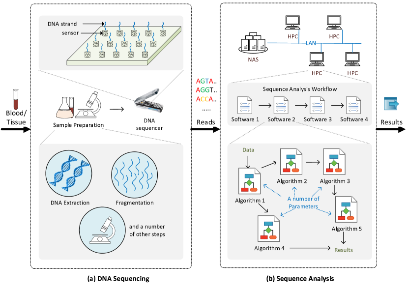
Figure 1.1: DNA sequencing and sequence analysis

Figure 1.2: Human DNA sequence printed as a series of books displayed at Wellcome Collection, Euston Square, London. Photograph from [11] licensed under Creative Commons Attribution-ShareAlike 2.0 Generic (CC BY-SA 2.0).

1. Reads are tiny compared to the original full DNA sequence (reads are around 75-500 bases in second-generation sequencers and around 1,000-100,000 bases in third-generation sequencers where the full DNA sequence is typically millions of bases long).

2. The reference sequence used for comparison is somewhat different to the DNA sequence in a sample (around 0.5% difference in humans due to genetic variation between two humans [12]) and the error caused by sequencers when reading the DNA is comparatively large (around 0.1%-1% in second-generation sequencers and around 0.5%-13% in third-generation sequencers).

3. The complexity of the human genome (i.e., more than 50% in the human DNA sequence are repeat regions [13, 14] and there are numerous types of repeat regions with distinct characteristics).

4. The large data volume output by the sequencers (can be as high as hundreds of gigabytes or even a few terabytes).

Over the last two decades, a plethora of workflows that perform DNA sequence analysis has emerged. A sequence analysis workflow is very sophisticated that a single workflow is a pipeline of different software tools run one after the other (Fig. 1.1) and each single software tool is a collection of numerous algorithms and heuristically determined parameters. Computational biologists or bioinformaticians have attempted to improve the accuracy of the sequence analysis workflows increasingly over the years, and as a result, the workflows have become more sophisticated.

1.1 Sequencers vs Computers - Gap Between Technologies

The rapid improvement in DNA sequencing technologies in terms of sequencing cost over the last two decades is depicted in the graph in Fig. 1.3. The hypothetical line that depicts Moore’s law is to compare how fast the sequencing technologies have improved. From 2001 to 2007, the cost of sequencing per human genome has reduced at a rate similar to Moore’s law. Then from 2007 to 2019, the drop in sequencing cost has been faster than Moore’s law, from 10 million USD to 1000 USD per human genome. Illumina, a leading sequencing company, has announced that their upcoming technology will bring down this cost to 100 USD in the future [5]. This rapid improvement is expected to continue and the sequencing machines which were limited to high-end research facilities are slowly arriving into pathology labs.

Figure 1.3: Drop of DNA sequencing cost per human genome over the period from 2001 to 2019. The Figure is from [15].

In addition to the improvement of DNA sequencing in terms of cost, the physical size and weight of the DNA sequencers also have improved. Fig. 1.4 shows the evolution of the sequencing machines over the last two decades. ABI Prison 3700 DNA sequencer, a first-generation sequencer released in 1999, was similar to the size of a fridge (dimensions 134.62 cm x 76.2 cm x 74.93 cm) with a weight over a hundred kilograms. Illumina MiSeq sequencer, a second-generation sequencer released in 2011 was the size of an oven (of the dimensions 68.6 cm × 56.5 cm × 52.3 cm) with a weight of 57.2 kg. The size further shrank with the Oxford Nanopore Technologies (ONT) MinION sequencer, a third-generation sequencer released in 2015 that is the size of a mobile phone (dimensions 10.5 cm x 2.3 cm x 3.3 cm and of weight 87 g). The size is expected to shrink further. Oxford Nanopore Technologies has already announced their upcoming product, ONT SmidgION, a tiny USB thumb drive sized DNA sequencer that could be directly plugged on to a mobile phone.

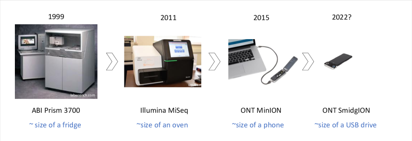
Figure 1.4: Evolution of sequencing machines

Although DNA sequencing has advanced rapidly, sequence analysis technologies are considerably lagging. As a result, even today, sequence analysis is typically performed on clusters of high-performance computers, the same situation as twenty years ago. There are multiple reasons for this lag, which are stated below.

1. General-purpose computers have not improved in terms of performance as fast as the DNA sequencers.

2. Data volume output by DNA sequencers has kept increasing despite the decrease in size.

3. The sophistication of the sequence analysis software tools also has increased over the years as a result of biologists improving the accuracy of the results.

4. Sequence analysis software tools written by computational biologists or bioinformaticians with the focus on higher accuracy of the results are un-optimised to efficiently utilise computational resources, i.e. software does not map well to the architecture of computers.

1.2 Need for Reducing the Gap

Sequence analysis steps consume days to weeks if done on a commodity laptop, or not possible at all in certain cases due to limited memory (RAM) in laptop computers. Hence, clusters of high-performance computers are currently being used, yet the process takes hours to complete. Such super-computers are very costly and massive and are typically available in high-end research facilities. As involved data set sizes are massive (can be up to several terabytes), cloud computing that relies on the internet is not ideal.

The utility of an ultra-portable DNA sequencer such as the MinION is currently limited due to the analysis process being performed on non-portable high-performance computers. There are a number of examples where scientists took these MinION sequencers into the field to perform sequencing. During the 2013-2016 Ebola virus outbreak in West Africa, scientists performed in-the-field sequencing using MinION sequencers [16]. However, the sequence analysis had to be performed offsite on high-performance computers in Europe. Gigabytes of data were transferred through a mobile internet connection which was expensive and slow. Analysis technologies to perform the analysis in-the-field would have been valuable in such circumstances, not only to reduce the cost but also for a quick turn-around time of results.

Another similar example is the use of the MinION during the Zika virus outbreak in Brazil [17], which the utility was again limited due to limitations in analysis technologies. Going beyond rural areas, scientists have performed sequencing using the MinION in jungles, arctic [18] and even on the international space station [19], which all of them would have benefited by efficient sequence analysis technologies. Currently, the ultra-portability of the MinION sequencer is being used to facilitate sequencing of the SARS-CoV-2 in smaller decentralised laboratories around the world [20]. Rapid epidemiological data sharing from places all over the world is a key to a better public health response. Having ultra-portable analysis technologies will further benefit in such circumstances.

Better analysis technologies will not only benefit portable applications such as the above but also in decentralising DNA tests in the future. DNA sequencers that are limited to high-end research facilities today will soon arrive in pathology labs and even doctor’s office. Having better sequence analysis technologies will support the data processing in situ without the need to transfer data to centralised high-performance computing facilities. Better sequence analysis technologies can also benefit large scale sequencing studies where the processing is performed in centralised high-performance computing facilities, by reducing the computing cost and the turnaround time of the results.

Considering all of the above factors, improving analysis technologies to match DNA sequencing technologies is a timely need.

1.3 Possible Solutions to Fill the Gap

Possible solutions to fill the gap between sequencing and analysis technologies are explored below in the context of the four reasons that were stated in the later part of section 1.1.

Performance of sequencers has evolved faster than computers that used to follow Moore’s law (Fig. 1.3). However, general-purpose single-core processor performance only improved by 3% in the year 2017—much slower than Moore’s law and future improvements should focus on application-specific hardware, as pointed by pioneers in computer architecture John Hennessy and David Patterson who received the Turing award in 2018 [21]. Application-Specific Integrated Circuits (ASIC) or custom circuit chips designed specifically for sequence analysis would be a potential solution to reduce the gap, which had already been applied as solutions in other domains such as digital signal processing. However, the field of genomics being still immature and thus the workflows rapidly evolving, designing custom hardware is challenging. Even little changes in algorithms require redesigning the custom hardware and this design cost is millions of dollars. An option that provides better flexibility than ASIC would be to design Application-Specific Instruction-set Processors (ASIP), which are in-between versions of general-purpose processors and ASICs in terms of flexibility. However, fabricating such ASIPs would still incur billions of dollars. Field Programmable Gate Arrays (FPGA) could be used as ‘breadboards‘ to prototype ASICs or ASIPS, however, full sequence analysis workflows are too complicated to be made fully functional on a typical FPGA with limited resources.

The high data volume output by the sequencers is a cause for an increased amount of computations, yet is beneficial to account for errors introduced by the sequencers, i.e, errors can be normalised when one region of a DNA string is covered by multiple reads. If sequencers become more and more accurate, the amount of data required to assemble a single DNA sequence will reduce. However, production of such accurate sensors that function at nano- and pico-scale measurements is far ahead in the future.

The complexity of the human genome is inevitable, i.e. there are seven categories of repeated sequences, each category has subcategories, each subcategory has a number of different families, each family has subfamilies and these subfamilies have distinct characteristics [22]. Also, more than 50% of the human genome is composed of repeated sequences [13, 14]. Certain regions (e.g. Telomere, Centromere) in the human genome have been too intractable to the existing technologies and are yet being resolved at the time of writing [23]. Analysis workflows that work on such complex genomes are thus inevitably sophisticated. What is meant by sophisticated here is not the algorithmic time-complexity, instead, the number of idiosyncratic cases that deviates from the general model. When processing, each of these deviated cases require to be separately handled. For instance, each family of repeated sequences would need to be processed using different algorithms and/or heuristic parameters, leading to a large number of code paths. A sequence analysis workflow as a whole would thus remain sophisticated, however, the time-complexity of each and every algorithm inside the workflow can be improved. Designing better algorithms with lesser time complexity has been and will be one of the most effective ways to improve performance. Over the past decades, plenty of work has been done in designing better algorithms and this will continue to happen.

Sequence analysis software tools are typically designed and developed by computational biologists or bioinformaticians whose major focus is to develop methods that are predicated on answering a research question or producing a specific outcome. Typically those computational biologists or bioinformaticians have access to near unlimited computational resources in their research environment—clusters of high-performance servers with hundreds of gigabytes of RAM. Their focus is not on maximal optimisation of the software, which requires detailed knowledge of computational systems. Consequently, sequence analysis software tools are typically severely un-optimised to efficiently run on computing systems with limited resources such as laptops or desktops. In other words, sequence analysis software tools severely lack computer architecture-aware optimisations that consider the knowledge of underlying hardware architecture. Note that these architecture-aware optimisations are not to be confused with algorithmic time-complexity optimisations which have already been done to a considerably adequate level in current sequence analysis software. Consider a hash table versus a contiguous array in memory. Despite accessing both the hash table and the array having the same time-complexity, contiguous accesses to an array are tens of times faster than random accesses to a hash table in a modern computer due to the presence of memory caches. Such optimisations that map existing sequence analysis software components to efficiently map with complex architectural features in modern computer systems are henceforth referred to as computer architecture-aware optimisations.

Out of the solutions discussed above, the most timely solution is to perform architecture-aware optimisations on existing sequence analysis software. Such optimisations are cost-effective and practical, yet rarely applied to sequence analysis software. The focus of this thesis is such architecture-aware optimisations on existing DNA sequence analysis software. In addition to the provision of efficient performance on general-purposes computers, such optimisations would complementary benefit any future-focused ASIP design efforts.

1.4 This Thesis

1.4.1 Philosophy

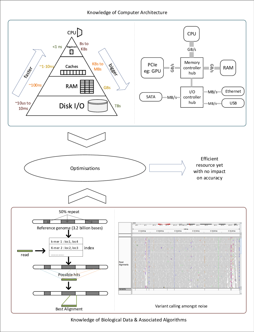
Figure 1.5: Synergistic use of knowledge from both computer architecture and biology

The architecture of modern computer systems is complex. Understanding such complex architectures requires the knowledge of a number of topics such as:

• the memory hierarchy (Fig. 1.5);

• interfacing between the processor, memory and co-processors (Fig. 1.5);

• internal details of processors and co-processors such as multiple cores, instruction scheduling and instructions set architecture; and,

• low-level software such as operating system (processes, threads, scheduling, disk caches, virtual memory, etc.) and device drivers.

Simultaneously, the field of DNA analysis is also utterly complex and understanding such analysis tools require knowledge of a number of topics such as:

• basic molecular biology involving the structure and function of DNA, chromosomes, genome, etc.;

• features of DNA sequences such as various types of repetitive sequences;

• different generations of DNA sequencing technologies;

• characteristics of data produced from sequencing technologies such as the read lengths and error rate; and,

• sequence analysis algorithms such as sequence alignment, variant calling and methylation calling.

Developing efficient software that conforms to hardware architectures requires the knowledge of all these computer architecture related topics. Developing sequence analysis software that produces accurate results require the knowledge of all above DNA analysis related topics. Thus, architecture-aware optimisation of sequence analysis software requires the simultaneous use of knowledge from both computer architecture and DNA analysis (Fig. 1.5).

DNA sequence analysis software tools are sophisticated and modern computer architectures are also sophisticated. Computer architecture knowledge helps to efficiently utilise resources. At the same time, knowledge of characteristics of biological data and associated algorithms ensures that the accuracy of the final results is unaffected. The domain knowledge from both the fields is utilised for the optimisations (Fig. 1.5). This thesis attempts to bridge the two interdisciplinary fields–computer architecture and DNA analysis—to produce sequence analysis software that can efficiently utilise existing resources in a modern computer system.

1.4.2 Chapter Outline

This thesis is about architecture-aware optimisations to existing DNA sequence analysis software. We present architecture-aware optimisations at different levels: Processor level, register level, cache level, RAM level and disk I/O level. The outline of the rest of the thesis is as follows.

In chapter 2, the background required to understand the technical chapters and a detailed literature review of the state-of-the-art are given. First, the background of DNA and DNA sequencing is presented in a simplified fashion for a reader from a non-biological background. Then, the background and the state-of-the-art of sequencing analysis workflows are presented. Finally, previous efforts of architecture-aware optimisation of DNA analysis workflows are presented.

In chapter 3, cache and register level optimisations to a popular variant calling software called Platypus are presented. A major time-consuming component of this software—de Bruijn Graph construction—was improved by a using cache and register level optimisations without any impact on the accuracy.

In chapter 4, memory (RAM) size optimisation of a popular sequence alignment software called Minimap2 is presented. The peak memory usage in Minimap2 was reduced through a divide and conquer strategy, most importantly, without compromising the accuracy. This work enabled performing sequence analysis in low memory systems such as mobile phones, which was otherwise not possible.

Chapter 5 discusses RAM level, cache level and processor level optimisations to a core algorithm component in analysing data produced from Oxford Nanopore sequencers called the Adaptive Banded Event Alignment (used in the popular Nanopore analysis toolkit Nanopolish). This includes how the algorithm was parallelised for CPU-GPU heterogeneous architectures. Importantly, the impact on the accuracy of the final results is negligible.

Chapter 6 discusses how the optimisations proposed in chapters 3,4,5 were integrated to develop fully functional embedded system prototypes for a popular nanopore sequence analysis workflow. It is shown the performance of the prototypical embedded systems employed with proposed optimisations is surprisingly comparable to the performance on the same workflow (unoptimised version) run on a high-performance server.

Then, going beyond embedded systems, chapter 7 presents the identification of the primary bottleneck in nanopore sequence analysis workflows that seriously affect high-performance servers. Solutions for alleviating this bottleneck are also presented.

Finally, the thesis is concluded in chapter 8 with a discussion of future directions.

1.4.3 Publications

Chapter 3 is published in IEEE/ACM transactions on computational biology and bioinformatics [24]. Chapter 4 is published in Nature Scientific Reports [25] and has received global attention amongst the community (altimeter score 89, picked up by 8 news outlets). Chapter 5 is available as a pre-print in bioRxiv [26] and a modified version is accepted for publication BMC Bioinformatics. Chapter 6 may be adapted for publication in the future. Chapter 7 is prepared to be submitted to an IEEE/ACM journal or conference proceedings.

In addition, collaborative research conducted in close relation to the work presented under this thesis has led to second author publications and pre-prints in [27, 28, 29]. However, none of the content from these second author publications is claimed as a part of this thesis.

1.4.4 Open-source Contributions

This thesis benefits the community through a number of contributions to existing open-source bioinformatics software and the development of new open-source bioinformatics software. Those existing open-source software tools that were contributed are Platypus variant caller (see chapter 3), popular sequence aligner Minimap2 (see chapter 4, appendix A and appendix G) and popular nanopore signal analysis toolkit Nanopolish (see appendix G). The new bioinformatics software developed under this thesis are f5c (see chapter 5, appendix B and appendix C) and f5p (see chapter 6 and appendix E). Also, the design and the associated software for the prototype embedded systems are released as open-source (see chapter 6 and appendix E).

1.4.5 Miscellaneous

The research conducted in support of this thesis has won third place in the grand final of ACM Student Research Competition 2020, amongst competitors from 22 major ACM conferences. The entry to the ACM SRC Grand finals was through winning the first place in ACM SRC at ESWEEK 2019 conference. Research conducted under this thesis has received the best poster award in Australasian Genomic Technologies Association Conference 2019.

Chapter 2 Literature Review

In this chapter, the background of DNA sequencing is discussed in section 2.1. Then, the background of sequence analysis and associated data structures and algorithms are discussed in section 2.2. In section 2.3, related work that has focused on computational optimisation of sequence analysis software is discussed.

2.1 DNA Sequencing

2.1.1 Terminology and Basics of DNA

In this subsection, the terminology in DNA sequencing and basic concepts of DNA sequencing are introduced.

2.1.1.1 DNA

Deoxyribonucleic Acid (DNA) is the blueprint of life. DNA is a molecule that encodes the structure and the function of a living organism [30]. A closer analogy from computer science is a computer program. A computer program is composed of instructions and data to achieve a particular outcome, whereas DNA is composed of instructions and data to make a living organism from scratch and to maintain its function. Instructions and data in a computer program are encoded in binary (base-2), whereas instructions and data in DNA are encoded in quaternary (base-4). The four bases in the DNA alphabet are Adenine (A), Cytosine (C), Guanine (G) and Thymine (T), which are molecules called nucleotides.

A long chain of nucleotide bases connected through chemical bonds forms a DNA strand. Two such strands that are coiled around each other, forming the double helix-shaped DNA molecule (Fig. 2.1). Both strands contain the same information and having two such strands facilitates DNA replication, the process by which DNA copies itself during cell division. The two strands are complementary to each other and are held together by hydrogen bonds between G-C and A-T base pairs, i.e., a base ‘G’ is complementary to base ‘C’ (and vice versa) and a base ‘A’ is complementary to base ‘T’ and vice versa).

2.1.1.2 Chromosome

A DNA molecule is tightly coiled many times and packaged with proteins to form a structure called a chromosome. Inside the nucleus of every cell of a human being, there are 23 pairs of such chromosomes (Fig. 2.1). Those chromosome pairs are named chromosome 1 to chromosome 22 and the 23^rd chromosome pair determines the sex. This 23^rd chromosome pair in females contains two X chromosomes and in males contains an X chromosome and a Y chromosome. In humans, the largest chromosome is chromosome 1 ($\sim$247 million bases) and the smallest is chromosome 21 ($\sim$47 million bases). In each chromosome pair, one chromosome is inherited from the mother and the other from the father.

The number of chromosomes varies amongst organisms. It can be just one chromosome or even thousands of chromosomes. The ploidy—whether the chromosomes exist in pairs, single or a higher number of sets—also varies amongst different organisms.

2.1.1.3 Genome

The complete nucleotide sequence of all the chromosomes within a cell is called the genome. The size of a genome is measured using the number of nucleotide bases. Following the metric prefixes, thousands of bases, millions of bases and billions of bases can be called kilobases, megabases and gigabases, respectively. Biologists typically use kb, Mb and Gb as symbols for those units, but this thesis uses the symbols kbases, Mbases and Gbases to prevent any confusion with kilobytes, megabytes and gigabytes.

The sizes of the genome of various organisms are listed in Table 2.1. Viral genomes are typically the smallest with a size of several thousand bases. Bacterial genomes can vary from several hundred thousand bases to a few million bases ($\sim$100 kbases to $\sim$15 Mbases). Insect genomes are in the order of hundreds of millions of bases ($\sim$100 Mbases to $\sim$900 Mbases). The genome size of complex organisms is billions of bases long. For instance, the human genome is 3.1 Gbases (6.2 Gbases if both chromosomes in a pair are considered). The largest genome found so far is of a rare Japanese flower plant called Paris japonica and is 149 Gbases long.

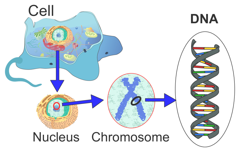
Figure 2.1: The DNA molecule and a chromosome. Chromosomes are present inside the nucleus of a cell of an organism. The DNA molecule that is the major component of a chromosome is double-stranded. A DNA strand is composed of four nucleotide bases A, C, G and T depicted in blue, yellow, red and green, respectively. The figure is from https://commons.wikimedia.org/wiki/File:Eukaryote_DNA.svg licensed under Creative Commons Attribution-Share Alike 3.0 Unported license.

Table 2.1: Genome size of various organisms

Organism	Genome size
HIV (virus)	10 kbases
H1N1 (virus)	14 kbases
SARS-CoV-2 (COVID-19 virus)	30 kbases
Helicobacter pylori (bacteria)	1.7 Mbases
Escherichia Coli (bacteria)	4.6 Mbases
Yeast	12.1 Mbases
Fruit fly (insect)	140 Mbases
Mouse	2.5 Gbases
Cow	3 Gbases
Human	3.1 Gbases
Wheat	17 Gbases
Marbled lungfish	130 Gbases
Paris japonica (plant)	149 Gbases

The widely used file format for storing a genome on a computer is the FASTA (.fa) format. FASTA is a simple text-based format where the characters ‘A’, ‘C’, ‘G’ and ‘T’ denote the nucleotide bases. An example genome stored in the FASTA format is given in Fig. 2.2. The line that starts with a ‘>’ character contains the name of the chromosome (may contain other metadata) and the subsequent lines contain the actual DNA sequence (Fig. 2.2).

To save space, FASTA can be compressed using the extended gzip format called bgzip that allows random access to genomic locations in the compressed file at the expense of a slightly lesser compression ratio than gzip.

Figure 2.2: An example of FASTA file format. The dotted lines are to indicate that the long chromosome sequences continue, i.e., dotted lines are not actually present in a FASTA file. Note that the sequences here are hypothetical and are not representative of a particular species.

A representative example of the genome of a particular species if known as the reference genome. Species such as humans have a high-quality reference as a result of the human genome project that produced a draft assembly, which was subsequently improved by scientists over the years. The latest version of the human genome is named as GRCh38 (Genome Reference Consortium Human Build 38).

2.1.1.4 Repeats

Repeats are quite common in genomes, for instance, more than 50% of the human genome is composed of repeats [13, 14]. Repeats are also known by terms such as repeated sequences, repetitive elements or repeat regions. Repeats have always introduced complications to the sequence analysis process, due to reads coming from such regions that are non-unique being extremely challenging to be accurately aligned [14].

Repeats have been classified into several types based on the characteristics of the sequence, for instance, satellite repeats, simple repeats, tandem repeats, transposons, etc. [31, 22].

2.1.1.5 Genes

The exact interpretation of the genome is not fully understood yet. However, scientists have interpreted the genome to a considerable extent. Millions of regions in the DNA called genes are individually or collectively responsible for features and functions of a living organism.

2.1.1.6 Variants

About 99.5% of the genome of all humans is the same [12]. The 0.5% difference encompasses human genetic variation. The differences in the genome of a particular individual to the reference genome of the particular species are called variants.

Different types of variants exist. A variation of a single nucleotide base is called a Single Nucleotide Variation (SNV). An SNV that is prevalent amongst a sufficiently large fraction of the population is referred to as Single Nucleotide Polymorphism (SNP). Insertion or deletion of one or more contiguous bases is called an Indel [32]. Examples of these three types of variants SNV, insertions and deletions are shown in Fig. 2.3. Indels can be small as one or two bases or large as ten thousand bases. Variants that are 50 or more bases (50 is the typical value and this number can be arbitrary) are known as structural variants [33]. Structural variants include many different sub-types such as long insertions, long deletions, copy number variants and inversions.

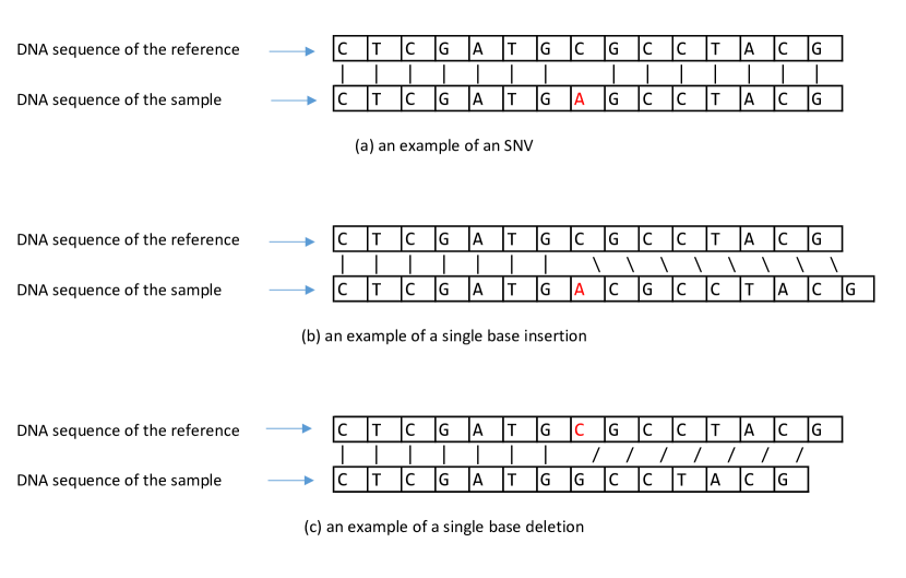
Figure 2.3: Elaboration of SNV and Indels

Most of these variants cause natural differences among individuals. However, some of the variants are responsible for various diseases. For instance, diseases such as sickle cell anaemia [34] and beta-thalassemia[35] are directly associated with SNVs. Diseases such as Asthma and Allergic Rhinitis are caused by a complex contribution of both genetic and environmental factors [36]. A large number of genetic variants that contribute to various diseases have been discovered. ClinVar is a public database containing such medically significant genetic variants [37]. More and more novel variants and their correspondence to various conditions are being readily discovered.

Detected variants are typically stored in the file format called Variant Call Format (VCF) [38], which is text-based format exemplified in Fig. 2.4. The header contains lines starting with ‘#’ character and describes metadata. Then, the details of variants are listed as tab-separated values with one variant per line.

Figure 2.4: An example of VCF file format

2.1.1.7 Epigenome

Nucleotide bases in the DNA can naturally undergo biochemical modifications when chemical compounds are attached to nucleotide bases. Such nucleotide bases with additional chemical compounds attached are known as modified bases. To date, more than 17 different types of base modifications have been identified in DNA [39]. The set of base modifications undergone by every base in the genome when taken together is called the epigenome. A common type of base modification in humans is the addition of methyl groups to nucleotide bases, which is known as DNA methylation.

DNA methylation is known to be a regulator of the genome, i.e., the expression of genes can be regulated by base modifications. DNA methylation is also known to affect development and tissue differentiation. DNA methylation is altered by environmental factors, but those alterations can be passed onto the next generations.

2.1.1.8 DNA Sequencing

The DNA molecule exists inside a human cell in a very compact form (scale of nanometres) with the DNA strand coiled many times, which if uncoiled would be a few metres long. To read the DNA strand, it has to be extracted from the cell and uncoiled. The DNA strand being very fragile when uncoiled, reading the full DNA strand from one end to another accurately is still a technological challenge. The best available technology today can only read this DNA strand in fragments of contiguous bases. This is due to the fragile DNA strand breaking into fragments at random locations during the DNA extraction process from the cell, uncoiling and even during the reading process. The process of reading the DNA sequence is termed DNA sequencing [40] and the machines that perform this sequencing are called DNA sequencers.

2.1.1.9 Reads

The sequencing machine takes a tissue sample of an organism, for instance, blood (more accurately a prepared sample out of tissue where the DNA strands have been extracted), and outputs the order of the bases in a digital form. The DNA strands break into fragments and the sequencing machine reads these fragments of DNA strands. The resultant series of data points denoting bases of a DNA fragment is called a read. The reads are output in random order by the sequencer. This is mainly due to the DNA fragments floating randomly in the liquid solution of the sample.

2.1.1.10 Coverage

A sample prepared for sequencing contains fragments of DNA that originated from nearly identical DNA molecules (each cell has a copy of the DNA and there are millions of cells in a sample). Fragmentation of DNA occurs at random locations on the DNA strand. The Sequencer randomly sequences a subset of these DNA fragments floating in the solution and outputs them as reads. Consequently, a single position in the genome is covered by multiple reads. The number of reads that overlap a particular position on the genome is known as the depth or coverage. Fig. 2.5 elaborates the coverage using an example. In the example, the coverage of the marked base position is 4$\times$ because the particular position on the original sequence is covered by four reads.

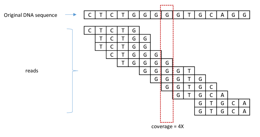
Figure 2.5: Elaboration of the concept of coverage in sequencing.

2.1.1.11 Base-calling

The process of converting direct or indirect measurements of the nucleotide bases (in the DNA strand) captured by sensors in the sequencer into ASCII reads is called base-calling. The base-calling process is not 100% accurate due to the presence of noise in measurements, sensor limitations and restrictions of the software involved in base-calling. One or more bases in a read can be incorrectly base-called and such errors are known as base-calling errors or sequencing errors.

The volume of data output by a sequencer or the sequencing yield is typically measured using the total number of bases in all the reads generated during a sequencing run (the duration in which the sequencing machine is operated). Modern sequencers can generate reads that sum to billions of bases and thus the common unit used for yield is Gbases.

Base-called reads are typically stored in the file format called FASTQ [41], a text-based file format extended from the previously discussed FASTA format. In FASTQ format, a single read takes four lines (Fig. 2.6): the first line is the read name (read identifier and optional metadata) that starts with an ‘@’ character; the second line is the actual read sequence in ACGT characters; the third line is always a ‘+’ character; and, the fourth line is the per-base phred quality score encoded in ASCII (phred quality score $Q$ is given by $Q=-10log_{10}(P)$ where $P$ is the base-calling error probabilities [42]).

Figure 2.6: An example of FASTQ file format

2.1.2 DNA Sequencing Technologies

As of today, there have been three generations of DNA sequencing technologies. They are detailed below.

2.1.2.1 First-Generation Sequencing

Sanger et al. used a method called the plus-minus system to sequence the first complete DNA which was of a virus in 1977 [43]. The introduction of the chain termination method (also known as Sanger Sequencing) [44] was a breakthrough in sequencing technologies due to its accuracy and convenience. With various improvements to this method, automated DNA sequencers were produced that were capable of sequencing complex genomes. These automated Sanger sequencers are known as first-generation sequencing machines.

First-generation sequencers can produce high-quality (accurate) long-reads at the expense of high cost and low throughput. For instance, Applied Biosystems 3730xl first-generation sequencer in Fig. 2.7 could output reads at around 99% accuracy and 400 to 900 bases length. However, a single sequencing run that spans over a duration of 20 minutes to 3 hours generates only 1.9-84 kbases [45]. In fact, the human genome project that started in 1990 mainly used first-generation sequencers [46]. The human genome project took 13 years to complete at an expense of billions of dollars. Today, first-generation sequencers are infrequently used.

Figure 2.7: First-generation sequencers. A row of Applied Biosystems 3730xl DNA Analyzer machines. Photo is from [47] licensed under CC BY 2.0. The weight of a machine is 180 kg and the dimensions are 100 cm (W) x 73 cm (D) x 89 cm (H) [48].

2.1.2.2 Second-Generation Sequencing

In 1985, a different technique to that used in first-generation sequencers was introduced [49] and the eventual improvements in the 1990s led to the second-generation sequencing technology. In literature, the term next-generation sequencing has been used instead of second-generation sequencing, which is no longer appropriate due to the emergence of the third-generation. Therefore, this thesis will continuously use the term second-generation sequencing.

Second-generation sequencers are capable of sequencing multiple DNA fragments (up to billions of fragments) in parallel and thus are also referred to using terms such as high-throughput sequencing or massively parallel sequencing. The sample preparation step for second-generation sequencing involves the intentional fragmentation of DNA strands into short pieces. The read lengths produced by second-generation sequencers are around 75-500 bases and these reads are referred to as short-reads. Second-generation sequencing has enabled sequencing complete genomes at an extremely low cost at a much faster rate when compared to first-generation sequencers. For instance, the Illumina X Ten sequencer was the first to achieve whole-genome sequencing (WGS) for 1000 USD in less than 3 days [50].

Illumina has become the dominant company in the production of second-generation sequencers. Illumina machines have an error rate of around 0.1%-1% per each base sequenced [51]. Fig. 2.8 depicts two different Illumina sequencing machines, HiSeq 2500 used in large-scale sequencing centres and Miseq that is a relatively smaller benchtop device.

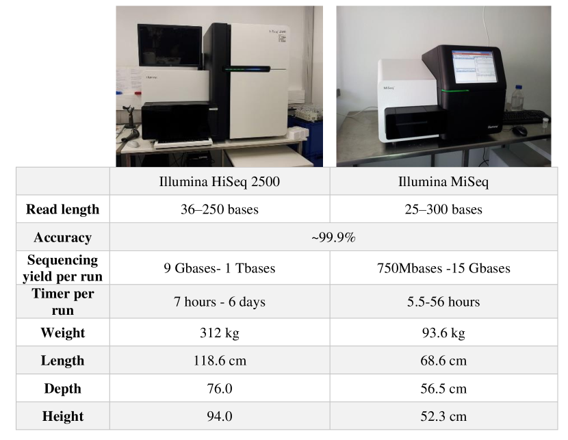
Figure 2.8: Illumina second-generation sequencers. Photograph of Hiseq sequencer is from https://commons.wikimedia.org/wiki/File:Illumina_HiSeq_2500.jpg and Miseq is from https://en.wikipedia.org/wiki/File:Illumina_MiSeq_sequencer.jpg, both licensed under CC0 1.0. Note that sequencing yield. Note that values for sequencing yield are to give a rough idea and may change based on a number of factors. Time of a sequencing run is given as a range since the exact value differs based on the configured value for the read length during sequencing.

Second-generation sequencers are widely used at present. Due to the low cost of sequencing with good accuracy, second-generation sequencers are suitable for SNV and short indel detection. However, the primary limitation of second-generation sequencing is that variants occurring in repeat regions of the genome cannot be easily resolved. This is because reads coming from such repeat regions usually align to multiple locations of the reference genome. Also, structural variants that are longer than the short-read lengths cannot be easily identified using second-generation sequencing.

Chapter 3 in this thesis is about software used to analyse second-generation sequencing data.

2.1.2.3 Third-Generation Sequencing

Sequencing approaches that are different from the second-generation sequencing appeared in the late 2000s and eventually led to the third-generation of sequencing technology [52]. Third-generation sequencers produce much longer reads with lower accuracy when compared to second-generation sequencers [53]. Reads produced by third-generation sequencers are known as long-reads. Similar to second-generation sequencers, third-generation sequencers are also capable of sequencing thousands of reads in parallel and thus fall under the category of high-throughput sequencers. Currently, two major companies produce third-generation sequencers. These are: Pacific Biosciences (PacBio); and, Oxford Nanopore Technologies (ONT). Third-generation sequencing technologies are under active development and are not as matured as second-generation sequencers. The read lengths and the accuracy are continually improving with time, and the values given here are to give a rough idea.

PacBio uses a technology known as Single-Molecule Realtime Sequencing (SMRT). Fig. 2.9 depicts one of their sequencers called Sequel. PacBio sequencers can produce reads under two distinct modes. These are Continuous Long-Reads (CLR); and, Circular Consensus Sequencing (CCS) reads. CLR are much longer (up to around 40 kbases) at the expense of lower accuracy ($\sim$87%), while CCS reads are more accurate ($\sim$99%), at comparatively shorter lengths (<2.5 kbases) at the time of writing[54].

Figure 2.9: Pacific Biosciences Sequel Sequencer. Photograph from https://en.wikipedia.org/wiki/File:SequelSequencer.jpg licensed under CC BY-SA 4.0. Dimensions are 92.7 x 86.4 x 167.6 cm

Oxford Nanopore Technologies (ONT) uses a technology known as nanopores. Nanopores are nanometre scale biological (protein) pores. Nanopore sequencers measure the ionic current when a DNA strand passes through a nanopore. The produced ionic current is in the range of pico-amperes and this instantaneous current varies based on the nucleotide bases inside the nanopore. Nanopore sequencers have hundreds of such nanopores and thus DNA strands are sequenced in parallel. The measured ionic currents are referred to as raw signals and are used during the base-calling process to deduce nucleotide sequences. Thus, nanopore sequencers are capable of directly measuring the actual DNA strand, unlike other sequencing technologies (second-generation Illumina or third-generation PacBio) that perform sequencing by synthesis.

The average length of reads produced by nanopore sequencers is typically 10-20 kbases, and the exact value of the length depends on fragmentation during sample preparation and the library preparation protocol. Ultra-long-reads that are longer than 1 Mbases have been recorded. The accuracy of raw base-called reads of Nanopore sequencers is $\sim$90-95% [55] and is constantly improving. Nanopore sequencers also output the raw signal data in addition to the base-called reads. This signal data can be used later during the sequence analysis process to reach a final consensus accuracy of $\sim$99.8% [56].

Currently, ONT produces three different sequencers as depicted in Fig. 2.10. MinION is the mobile phone-sized ultra-portable sequencer for in-the-field sequencing. GridION is a bench-top sequencer and is equivalent to five MinIONs in sequencing capacity. PromethION is for massive scale sequencing facilities and is capable of sequencing up to about 48 human genomes in parallel.

The MinIONs sequencer in Fig. 2.10 does not have a built-in computing unit for base-calling. Thus, the base-calling had to be performed on a workstation or a laptop. ONT recently released (in 2018) an ultra-portable compute module called MinIT that is directly pluggable to the ultra-portable MinION (Fig. 2.11(a)) to make the base-calling process ultra-portable. In addition, ONT very recently (in 2019) released the next version of the MinION sequencer called MinION Mk1C that has an integrated base-calling compute module (Fig. 2.11(c)). GridION (Fig. 2.10) has a built-in computing unit composed of GPUs for base-calling. The PromethION sequencer comes with a computer tower (high-end workstation) to be used for base-calling (Fig. 2.11(b)).

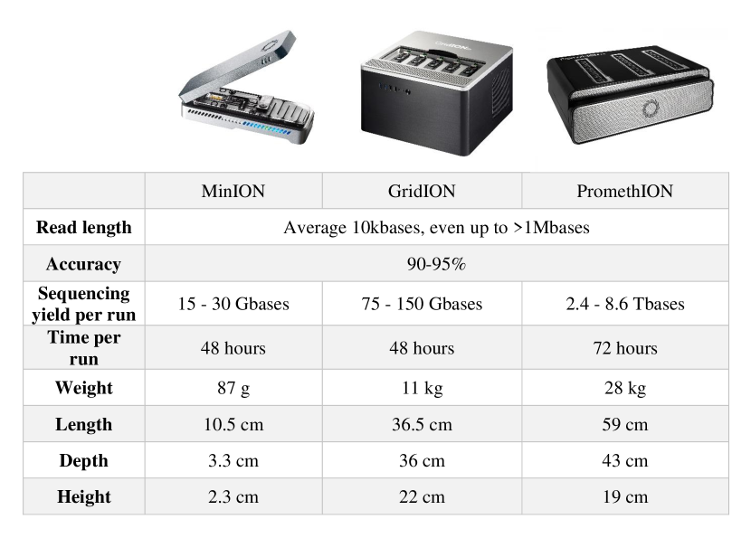
Figure 2.10: Nanopore third-generation sequencers. The photographs are from Nanopore https://nanoporetech.com/about-us/for-the-media. The read lengths and the sequencing yields values are for the purpose of giving a rough idea and may change on a variety of different factors.

(a) MinION sequencer (right) connected to the MinIT base-calling unit (left)

(b) PromethION sequencer (left) and its compute tower (right)

(c) MinION Mk1C sequencer with integrated base-calling unit

Figure 2.11: ONT MinIT, PromethION compute tower and MinION Mk1C. The photographs are from Nanopore https://nanoporetech.com/about-us/for-the-media.

Third-generation sequencers are mainly used by researchers for detecting structural variants and resolving complex and highly repetitive regions that were not possible with the read lengths of previous generation sequencers. For instance, 29 unresolved regions of the X chromosome of the human genome reference were only resolved very recently using third-generation sequencing technology [23].

Unlike other technologies, Nanopore sequencers can stream data in real-time which facilitates data analysis on-the-fly (while the sequencer is operating). Also, Nanopore sequencers such as the MinION are ultra-portable, and they are in harmony with the intention of this thesis to construct embedded systems for sequence analysis.

2.2 Sequence Analysis

The goal of sequence analysis is to: assemble the reads into the actual DNA sequence in the sample (or the genome); or, to compare differences in the reads to a reference genome (e.g., to detect variants or epigenetic modifications). The former is performed when a high-quality reference genome is not available and thus the assembly has to be performed from the scratch (known as de novo assembly). The latter performed When a high-quality reference genome is available (referred to as reference-guided sequence analysis). This thesis focuses on reference-guided sequence analysis. For well-known species like humans, scientists have spent years compiling a high-quality reference sequence. Therefore, for most practical purposes involving humans, reference-guided sequence analysis is adequate.

While the reference-guided sequence analysis has some similarities between second-generation and third-generation sequencing, there are important differences. Section 2.2.1, describes the typical reference-guided sequence analysis workflow for second-generation sequencing and section 2.2.2 for third-generation sequencing. Despite being not required for the thesis, a brief account of de novo assembly is given in section 2.2.3 for the sake of completeness.

2.2.1 Reference-guided second-generation workflow

A simplified second-generation bioinformatics workflow is given in Fig. 2.12. Certain workflows may contain additional steps such as filtering and calibration (i.e. GATK Best Practices pipeline from Broad institute in Fig. 2.13). However, the most important and computationally challenging steps are the ones shown in Fig. 2.12.

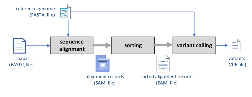
Figure 2.12: Simplified second-generation workflow

Figure 2.13: GATK Best Practices pipeline. Image from https://gatk.broadinstitute.org

The reads, typically in FASTQ format (discussed previously in section 2.1.1.11), are first aligned to the reference genome (step one in Fig. 2.12). This process is known by various terms such as sequence alignment, read alignment or read mapping. Sequence alignment process produces the alignment records for every read (whether the read was successfully mapped, mapping coordinates, mapping quality, etc.), in a file format called sequence alignment/map format (SAM) [57]. Tools and associated algorithms for sequence alignment are detailed in section 2.2.1.1.

The alignment records in the SAM file are then sorted (step two in Fig. 2.12) based on genomic coordinates. That is, sorting first by chromosome order and then by base position in each chromosome. The sorted alignment records are typically stored in a file format called BAM, which is a binary version of SAM format with BGZF compression support [57]. BAM allows random accesses to alignment records for a given genomics region through an index called the BAM index. The most popular tool for sorting is samtools [57] written in C programming language, which is reasonably optimised for performance. Other tools such as Picard [58] written in Java programming language and Sambamba [59] written in D programming language can also be used for sorting.

The next step is the identification of variants amongst sequencing errors and alignment artefacts, and this process is known as variant calling (step three in Fig. 2.12). The variant calling step takes the sorted alignment records (BAM file) and the reference genome (FASTA file) and outputs the identified variants in VCF file format (discussed previously in section 2.1.1.6). These variants can reveal important information about the individual, such as disease predisposition and drug response. However, variant calling is quite challenging as variants should be differentiated correctly from sequencing errors and alignment artefacts. Tools and associated algorithms for variant calling are detailed in section 2.2.1.2.

2.2.1.1 Sequence Alignment

Fig. 2.14 is a simplified elaboration of sequence alignment. Sixteen reads with read lengths of 8 bases have been aligned to the reference. The differences in the reads to the reference (due to sequencing errors or actual variants) have been shaded in grey. Note that, only single base mismatches are in this demonstration, where in reality there can be insertions and deletions. The average number of reads that overlaps a particular nucleotide position is called coverage. Terms such as depth and depth of coverage are also interchangeably used [60]. The required coverage depends on the application [60], for instance, a coverage of 30X or more is recommended [61] for detection of SNV and indels.

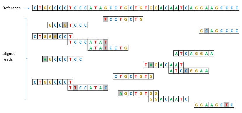
Figure 2.14: Simplified illustration of aligned sequence reads to a reference

To date, a large number of sequence alignment tools have been published [62]. Modern sequence alignment tools typically perform the alignment in two steps: first, potential mapping locations of a given read on the reference genome are searched using an index (e.g. hash table); and second, the read is aligned at base-level to those potential locations in the reference using dynamic programming-based alignment algorithms to identify the optimal alignment.

Use of an index is required to reduce the search space in a large genome. Performing base-level alignment of a read on to the whole reference genome is impractical due to computational and memory complexity when the reference genome is large. Locating a few locations on the reference genome (for instance 5-10) using an index is thus vital. The two common indexing approaches use hash tables and the Burrows-Wheeler transform (BWT) [63].

Earlier short-read alignment tools used the hash table-based approach. The alignment tool MAQ [64] builds a hash table out of the reads and iterate through the reference sequence to find potential mappings. In contrast, alignment tools such as SOAP [65] and BFAST [66] build the hash table using the reference genome and iterate through the reads to find potential mappings.

Modern short-read alignments tools typically rely on a BWT-based index called an FM-index [67]. An FM-index is constructed by taking the BWT of the reference genome, which effectively compresses the data while allowing sub-string indexing at the same time. The FM-index-based approach has gained popularity due to its superiority to hash tables in terms of both performance and memory footprint. Alignment tools such as BOWTIE [68, 69], BWA [70, 71, 72] and SOAP2 [73] use this approach.

After potential mapping locations are identified quickly using an index, more accurate base-level alignment algorithms are dispatched to find the optimal alignment. These algorithms to determine the optimal alignment between two biological sequences typically utilise dynamic programming (DP). Very first of such algorithms, the Needleman-Wunsch (NW) algorithm dates back to the 1970s [74]. NW and its variant, the Smith-Waterman (SW) algorithm [75] are of quadratic time and space complexity. Both NW and SW were used extensively to perform fine alignment of DNA sequences with high quality. However, due to its extended time consumption, several heuristic improvements have been proposed by researchers to improve the speed of alignment without losing quality.

Fig. 2.15(a) exemplifies an original SW based alignment (no heuristic) between two sequences, target sequence t₀t₁t₂t₃t₄t₅ (6 bases long), and query sequence q₀q₁q₂q₃q₄q₅q₆q₇ (8 bases long). The DP table (scoring matrix) contains 6x8 cells as shown. First, the initial values are set (shown as 0 in the figure); second, the score for each cell (s_x,y) is computed based on a scoring scheme; and third, the trace-back (backtracking denoted by red arrows on the figure) starting from the highest-scoring cell and ending at a cell with 0 score, outputs the optimal alignment that yields the highest score (please refer [76] for a detailed explanation of SW).

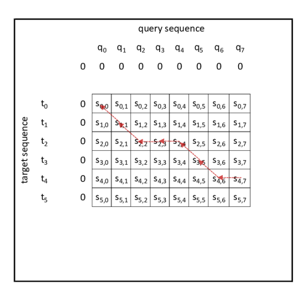
(a) optimal sequence alignment

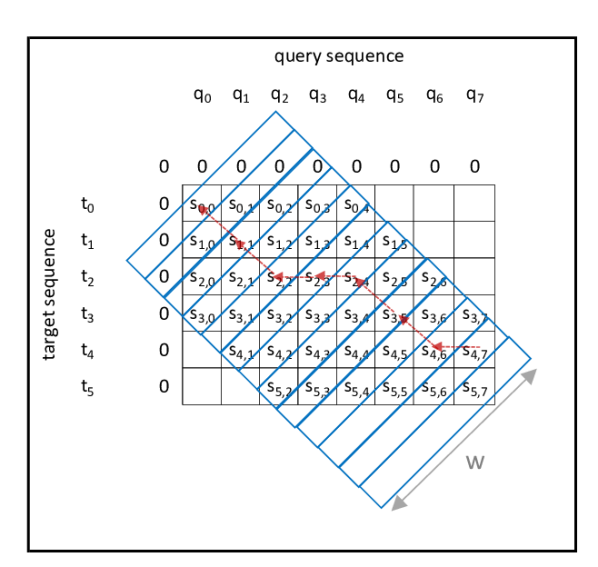
(b) Banded sequence alignment (band-width=4)

Figure 2.15: Dynamic programming based sequence alignment

In the case of short-read alignment, the sequences to be aligned are small (typically 75-500 bases). Two sequences (each sequence ~100 bases long) can be aligned by filling ~10⁴ cells. While a single such alignment can be quickly handled by a modern computer, it is computationally demanding when the number of alignments to be performed scales up to hundreds of millions and billions, which is the case for short-reads. To reduce the number of computations, banded alignment approaches were introduced [77], where only the cells in the DP table along the left diagonal band are computed as shown in Fig. 2.15(b). The underlying assumption is that the sequences that are aligned to each other are essentially similar, thus the alignment (the trace-back arrows) should lie close to the left diagonal. Note that in the figure, only the cells in a band of width (W) four have been computed. This computation is sufficient since the band contains the alignment.

X-drop in BLAST (Basic Local Alignment Search Tool) [78] is another notable heuristic to SW that terminates the computation when the drop in the alignment score reaches a threshold. An extended version of X-drop called Z-drop is used in the modern alignment tool BWA MEM [72].

In addition to computing the alignment and the alignment score for each read, modern alignment tools also compute an important quantity called the Mapping Quality (MAPQ). The concept of mapping quality was introduced in MAQ aligner [64]. MAPQ is computed per read as: $−10log_{10}(P)$ rounded off to the nearest integer, where $P$ is the probability of the mapping position being incorrect. This probability value is heuristically determined through different formulas in different software but essentially considers both the alignment score and the number of sub-optimal mappings of the read. A higher number of sub-optimal mappings means that the read is likely to be from a repeat sequence and thus the chance of being incorrect is high. MAPQ is an important score for the variant calling step, i.e., to avoid false-positive variants.

2.2.1.2 Variant Calling

Variant calling is the process of identifying the variants amongst sequencing errors and alignment artefacts. One of the simplest possible examples illustrating the variant calling process in Fig. 2.16, which is based on the same reads and the reference used in the previous example (Fig. 2.14). Note that in Fig. 2.16, the reads have been sorted based on genomic coordinates and the marked variant is simply based on the majority vote. However, such a simple strategy will not be adequate for accurately identifying variants in real genomic data (to minimise both false positives and false negatives) and numerous sophisticated variant calling software tools have been introduced.

More than 40 open source tools have been released in the last decade [79]. Most tools utilise a probabilistic framework (Bayesian approach is the most common) and popular variant calling tools such as GATK UnifiedGenotyper [80], GATK HaplotypeCaller [81] (the of UnifiedGenotyper), FreeBayes [82], SAMtools package (samtools and bcftools) [83] and Platypus [84] are some examples. In contrast to the probabilistic methods, certain tools such as VarScan rely on heuristic approaches [85, 86].

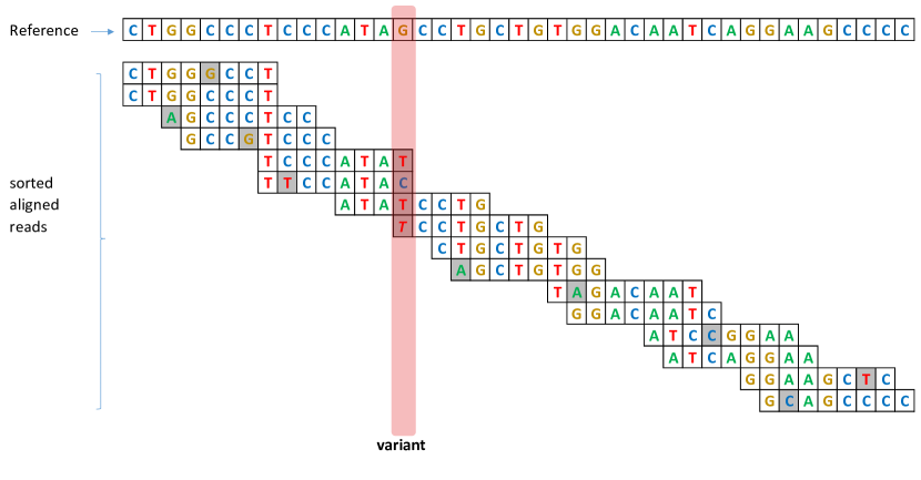
Figure 2.16: Simplified elaboration of variant calling

Past variant callers (e.g, GATK UnifiedGenotyper) solely relied on the read alignment performed by the aligning tool. However, alignment artefacts due to indels were found to affect the accuracy of the variants calling results [87]. Thus, separate pre-processing tools such as GATK IndelRealigner were introduced to perform local re-alignment in the affected regions [88] before executing the variant caller. Modern variant calling tools such as GATK HaplotypeCaller and Platypus have a built-in local de novo assembly step to address the aforementioned issue, making GATK IndelRealigner redundant. In local de novo assembly, the genome is broken into small regions and de novo assembly is performed separately in these regions. For local de novo assembly, Platypus uses a variant of Bruijn graphs called coloured de Bruijn graphs [89], while GATK HaplotypeCaller also uses a de Bruijn like graph [90].

In the past variant callers (e.g, GATK UnifiedGenotyper), each base position on the genome was considered independently when calculating probabilities. However, recent variant callers such as GATK HaplotypeCaller and Platypus breaks the genome into overlapping haplotypes based on initially identified variations. They perform probability calculation on these haplotypes by mapping reads to each haplotype. GATK HaplotypeCaller uses pair Hidden Markov Model (pairHMM) [91] and Platypus uses Needleman-Wunch for mapping reads to haplotypes. Haplotype-based approaches have increased the accuracy of variant calls [92].

Sandmann et al. [79] evaluated the accuracy of eight variant calling tools including GATK, Platypus and SAMtools. None of the variant callers could detect all the variants in their data sets. They also observed that increased sensitivity decreases precision. Further, the accuracy of different tools varied with different data sets. Hence, modern variant calling tools are being frequently updated to gradually improve accuracy.

Variant calling is a time-consuming step that takes hours on a high-performance computer. Despite this, many variant callers such as VarScan, FreeBayes, SNVer [85] and VarDict [93] do not support multi-threading. GATK HaplotypeCaller does support multi-threading. However, multi-threaded executions of GATK HapplotypeCaller frequently crash and thus are not recommended to be used as stated in the manual [94]. Even during instances that do not crash, the multi-threaded execution of GATK HaplotypeCaller marginally improves the run-time due to inefficient multi-core utilisation. Further, multi-threaded execution could not reproduce the same result as single-threaded execution as observed by Sandmann et al. [79]. Platypus variant caller is capable of efficiently utilising multi-CPU cores through its in-built multi-processing.

Chapter 3 describes memory optimisation algorithms associated with variant calling. Specific details of the underlying algorithms are discussed in the background of that chapter.

2.2.1.3 Characteristics of data

Read length: In a second-generation sequencing dataset, the lengths of all the reads in the dataset are typically the same (at least for Illumina Sequencing that dominates the second-generation sequencing market). The read length can be initially configured to a particular value between around 50 and 500 bases at the start of a sequencing run (depending on the sequencing machine) and all the reads generated from that sequencing run would of that configured length.

Error rate: An example demonstrating the error rate of second-generation sequencing is in Fig. 2.17. This example uses Illumina short-reads from a real dataset (NA12878 dataset from 1000 genomes project) aligned to a reference (human genome). Fig. 2.17 is a screenshot of a $\sim$6 kbase region in chromosome 22 taken through the Interactive Genome Viewer (IGV). The grey colour horizontal blocks on Fig. 2.17 represent the reads and other colours represent differences in those reads to the reference. The bottom panel shows the variants that are present in this region.

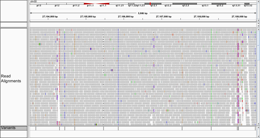
Figure 2.17: A screenshot from IGV for the region chr22:27,103,514-27,109,534 from an NA12878 dataset aligned to the human genome

Data size: The human genome is 3.1 Gbases and the FASTA file (uncompressed) is around 3.1 GB. If the human genome is sequenced at an average coverage of 30X, the yield is around 96 Gbases. If the read length is assumed to be 100, the dataset would contain around 960 million reads. A FASTQ file (uncompressed) storing such a dataset is around 200-250 GB. The generated result from the alignment step stored in a SAM file (uncompressed) is around 250-300 GB. The sorted alignments stored as a BAM file (BGZF compressed) is around 30-40 GB. The VCF file generated from the variant calling step is around 1 GB.

2.2.2 Reference-guided third-generation workflow for nanopore data

Third-generation sequencing technology is currently under active development and no standard or best practises workflow exists at present (as opposed to the second-generation). Third-generation sequencing workflows are not stable and are constantly evolving. Fig. 2.18 shows the typical workflow for nanopore data processing at the time of writing.

The reads (in FASTQ file format) are first aligned to the reference genome (step one in Fig. 2.18). The alignment is conceptually similar to that of the second-generation workflow. However, software tools used for aligning third-generation sequencing have distinct characteristics which are different from the previous aligners and are detailed in section 2.2.2.1. After the alignment step, the aligned reads are sorted (step two in Fig. 2.18). The sorting step is identical to that of the second-generation workflow and the most popular sorting tool remains Samtools. The next step (step three labelled as polishing in Fig. 2.18) now can be either variant calling or detection of epigenetic base modifications (e.g., methylation calling). Variant calling or detection of epigenetic base modifications is a challenging process where true variants and/or base modifications must be identified amongst highly erroneous reads (currently 5%-10%). Thus, this step typically uses the raw signals (raw sensor output from the sequencer) in addition to the base-called reads. Associated software tools for variant calling and detection of epigenetic base modifications are detailed in section 2.2.2.2.

As stated in section 2.1.2.3, a raw signal is the ionic current measurement when a DNA strand passes through a protein nanopore. Nanopore sequencers output these raw signals in a file format called fast5. Fast5 format is essentially the Hierarchical Data Format 5 (HDF5) [95], with a specific scheme determined by ONT to store raw signal data and metadata. Before 2018, a single raw signal (corresponds to a single read) was stored as a single fast5 file, which is currently referred to as a single-fast5 file. However, millions of files generated from a sequencing run were difficult to manage and now a fast5 file contains a batch of raw signals (by default 4000 reads). Such fast5 files containing multiple reads are called multi-fast5 files. HDF5 is a versatile file format with numerous features (including compression). However, HDF5 is a very complicated file format of a monolithic design and a lengthy specification. Consequently, HDF5 files must be accessed through the only existing library provided by the HDF5 group, which has limitations such as lack of efficient multi-threading access. Chapter 7 of this thesis explores the impact of this limitation on efficient raw signal access and presents alternate solutions to circumvent the limitation.

As nanopore sequencers output raw signals, base-calling can be optionally performed externally on a general-purpose computer. However, the latest nanopore sequencers either come with an internal compute-module or support an externally attachable dedicated base-calling module running ONT’s proprietary base-callers. Thus, base-calling will not be considered under sequence analysis in this thesis.

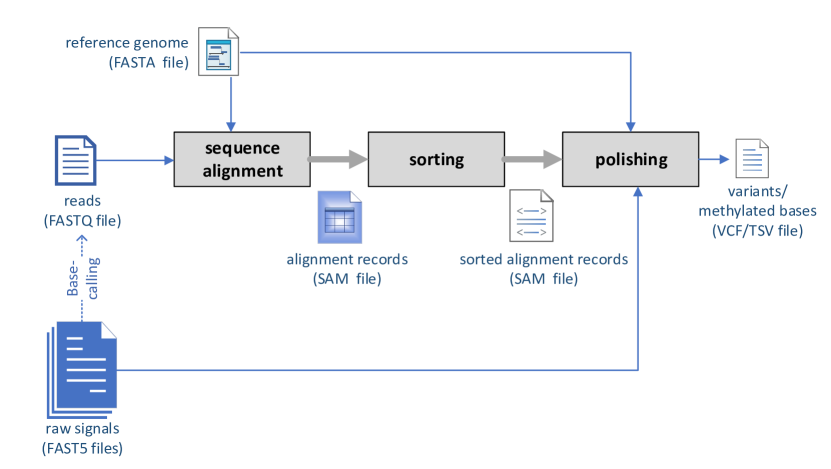
Figure 2.18: Simplified third-generation nanopore workflow

2.2.2.1 Sequence Alignment

When examined from a higher level, long-read aligners also use a two-step approach similar to previous aligners: finding potential mapping locations using an index; and, applying accurate dynamic programming algorithms to obtain the optimal alignment. However, when looked microscopically, long-reads aligners have major differences in underlying algorithms and parameters to handle distinct characteristics of long-reads. Numerous long-read aligners have been published over the last decade, for instance, BWA MEM [72], BLASR [96], GraphMap [97], Kart [98], NGMLR [99], LAMSA [100] and Minimap2[101]. Note that BWA MEM is an extended version of previously discussed BWA (BWA was initially designed for short-reads), that supports long-reads up to a certain degree. Minimap2[101] is the most popular long-read aligner amongst all the other long-read aligners, due to its superior performance, accuracy and robustness. Minimap2 [101] employs a hash table-based genome index to quickly locate potential mappings and is both fast and accurate compared to the FM-index-based approach in BWA MEM [72]. However, the RAM requirement is higher for a hash table-based index compared to FM-index. For instance, The hash table data structure itself consumes about 8 GB of memory (RAM) in Minimap2. The typically RAM consumption of Minimap2 is around 12 GB on average when memory is allocated for internal data structures (i.e. dynamic programming tables). However, the peak RAM for the human genome can occasionally exceed 16 GB depending on the characteristics of data, such as the length of the reads. Chapter 4 of this thesis focuses on memory optimisations to Minimap2 to reduce peak RAM.

Banded versions of dynamic programming algorithms such as SW and NW (fig) used for short-reads are not directly suitable for long-reads. In contrast to short-reads, the long-reads which emanate from Nanopore, PacBio etc, have lengths which are 10 to 10000 orders of magnitude bigger than short-reads, are noisier (with a greater number of errors) and are typically not suitable for such small static bands. The 10% base-calling error rate would result in the alignment significantly deviating from the diagonal (diagonal mentioned in section 2.2.1.1). A major advantage of long-reads is the detection of long indels (insertions and deletions occasionally spanning lengths longer than short-reads themselves). When aligning such reads, the alignment path deviates significantly from the diagonal. The high errors and the large indels require the bands to be of large width if they are to be static. High bandwidth requirement causes processing times to be extremely high when aligning millions of reads. To improve the speed of this processing, Suzuki-Kasahara (SK) heuristic algorithm [102] was introduced in 2017. SK utilises an adaptive band scheme, letting a smaller band to contain such an alignment within the band, which is exemplified as below.

Consider the same example in Fig. 2.15(b) (performed previously with a static band of size 4) is now performed only with a band-width of size 3, as shown the Fig. 2.19(a). Observe that the band is no longer sufficient to contain the whole alignment, i.e. the cell s_4,7 which previously contained the maximum score is no longer computed, thus the trace-back would begin from the maximum value within the band, which leads to a non-optimal alignment. This is remedied using an adaptive band in Fig. 2.19(b). The band moves either down or to the right (the band dynamically adapts) as determined by the Suzuki-Kasahara heuristic, which is illustrated by blue arrows. Observe how the alignment is possible to be contained inside a band of width 3 which was previously infeasible using a static band.

(a) Banded sequence alignment (band-width=3)

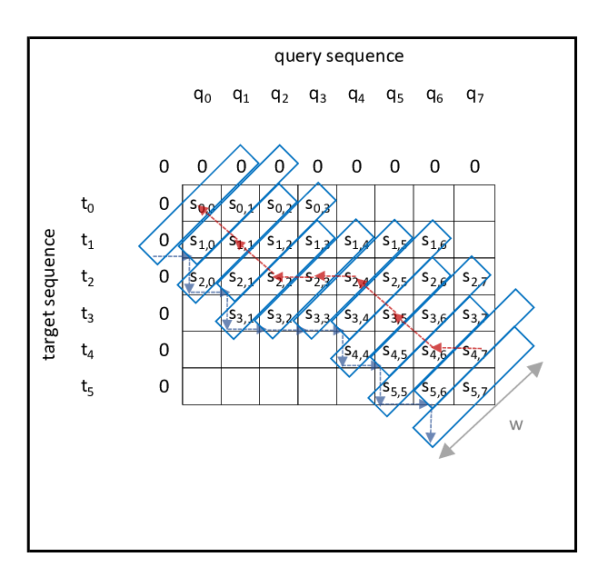
(b) Adaptive banded sequence alignment

Figure 2.19: Evolution of dynamic programming-based sequence alignment

2.2.2.2 Variant calling / detection of epigenetic base modifications

As stated before, variant calling or detection of epigenetic base modifications is a downstream processing step which utilises both base-space alignments and raw signals. This step reuses the raw signals to recover the lost biological information during base-calling. Previous research [56, 103] has shown that the identification of genetic variants can be improved up to an accuracy of more than 99% by using raw signal data from multiple overlapping nanopore reads. It has also been shown that methylated C bases can be differentiated from non-methylated C bases by the use of signal data, using algorithms such as the one implemented in the software package Nanopolish [104]. Thus, the downstream analysis that reuses raw signal data could also detect modified nucleotide bases.

At the time of writing Nanopolish [104] is the most popular software package amongst the nanopore community for variant calling and detection of epigenetic base modifications. Nanopolish takes the reads, their alignments to the reference genome and the raw signal of each read as the input. Initially, the raw signal is segmented in the time domain based on sudden jumps in the signal and these segments are known as events. The events are then aligned to a hypothetical signal model using an algorithm called Adaptive Banded Event Alignment (ABEA). The output of ABEA and alignment details of reads to the reference genome are sent through a Hidden Markov Model (HMM) to detect variants or base modifications. Nanopolish is written in C/C++ and supports multi-threading through openMP. Chapter 5 of this thesis is about the optimisation of Nanopolish (ABEA algorithm in particular) and details of the algorithm are discussed in the background of that chapter.

Tombo is another software for detection of modified bases which also uses raw signals for the process. Tombo has been developed in Python programming language. Recently, a few neural network-based variant callers also have been released, for instance, Medaka[105], Clairvoyante [106] and Clair [107] (successor of Medaka Clairvoyante). These neural network-based variant callers have been developed in Python programming language and use Tensorflow in the backend. Unlike Nanopolish, these neural network-based variant callers only rely on base-called reads and are incapable of using raw signal data.

2.2.2.3 Characteristics of data

Read length: In third-generation sequencing, read lengths can significantly vary within a dataset. For instance, read lengths can be from a few hundred bases to >1 Mbases in nanopore sequencing. Fig. 2.20 shows read length distributions of nine datasets, out of the 53 publicly available NA12878 datasets (different datasets produced at different sequencing run of the NA12878 sample) from the nanopore consortium [56]. The library preparation method is a major factor that affects the read lengths. Currently, there are three library preparation method for nanopore, ligation and rapid, which are officially from Oxford Nanopore, and Ultra which is community-developed [56]. Fig. 2.20 shows three datasets from each of those library preparation methods and demonstrates that the read length distributions vary not only among different library preparation methods but also among different datasets from the same library preparation method.

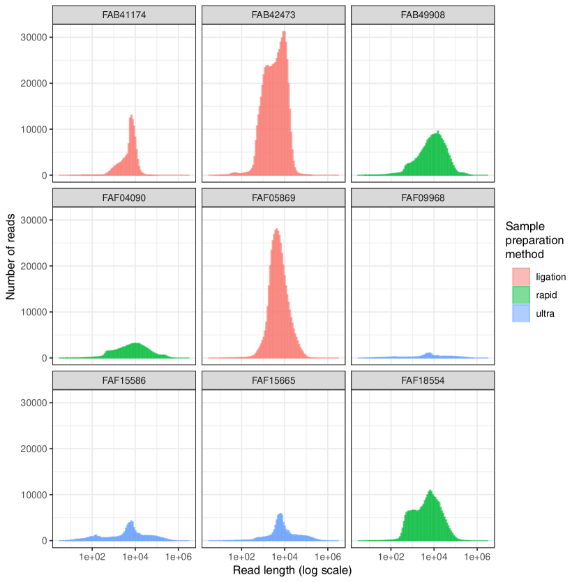
Figure 2.20: Read length distribution nanopore consortium

Error rate: The error rate of nanopore third-generation sequencing is demonstrated in Fig. 2.21 using reads from a real dataset (all NA12878 data from nanopore consortium [56]) aligned to a reference (human genome). Fig. 2.21 is a screenshot of a $\sim$6 kbase region in chromosome 22 taken through the Interactive Genome Viewer (IGV). Similar to Fig. 2.17 for second-generation sequencing, the grey colour horizontal blocks on Fig. 2.21 represent the reads and other colours represent differences in those reads to the reference. The bottom panel shows the variants that are present in this region. Observe how high the error rate in third-generation sequencing (Fig. 2.21) is, compared to second-generation sequencing (Fig. 2.17).

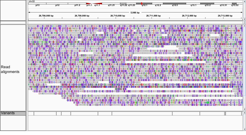
Figure 2.21: A screenshot from IGV for a region from NA12878 sample nanopore consortium genome project

Data size: When all NA12878 datasets from the nanopore consortium are aggregated, the total is around 132.931 Gbases. This is equivalent to about 40X coverage of the human genome. The number of reads is 15.667 million. The FASTQ (uncompressed) file containing these read is 250GB in size. The SAM file (uncompressed) generated by aligning these reads using Minimap2 is 280 GB. The sorted BAM file (compressed) is around 150 GB. Per-read methylation calls generated from nanopolish which are in TSV format (uncompressed) consume around 70 GB. The VCF file generated from the variant calling step is around 1 GB. Raw signals corresponding to the aforementioned reads stored in the latest fast5 format (multi-fast5 with compression) consume around 2.2 TB. Note that this used to be 46 TB a few years ago when stored as single-fast files (mostly due to redundant data such as the event table).

2.2.3 De novo assembly

If it is the first time that the DNA of the particular species is sequenced, then the reads must be assembled without any reference, only using the information in the reads. This process is known as de novo assembly.

Early de novo assemblers such as SEQAID [108] were based on greedy algorithms. Modern assemblers rely on graph-based techniques. Short-read assemblers mostly use de Bruijn graphs [109] and examples are ABySS [110], Velvet [109], Spades [111] and Cortex [112] use de Bruijn graphs. However, SGA [113] which is also a short-read assembler uses overlap graphs (a type of overlap called string graphs [114]). Almost all long-read assemblers use overlap graph-based methods. Examples of long-read aligners are miniasm [115], flye [116], canu [117] and wtdbg2 [118].

Currently, there are three de novo assembly workflows: 1, using only short-reads; 2, using only long-reads; and, 3, using both called hybrid assembly. For more information of de novo assembly readers may refer to [29].

2.3 Architecture-aware optimisation of sequence analysis algorithms

Studies in the field of DNA analysis have predominantly focused on improving the accuracy of algorithms. Such improvements have further increased the computing power required for the analysis. Compared to the plethora of studies focusing on accuracy, studies attempting to reduce the gap between DNA sequencing and analysis technologies (architecture-aware optimisation of sequence analysis algorithms) are minimal. This section presents those architecture-aware optimisation studies under four categories: work that optimises sequence analysis algorithms for general-purpose CPU, HPC, cloud computing and distributed computing in section 2.3.1; work on GPU-based optimisations in section 2.3.2; FPGA-based optimisations in section 2.3.3; and, specialised hardware design for sequence analysis in section 2.3.4.

2.3.1 CPU/HPC/Cloud

Core sequence alignment algorithms for second-generation sequencing such as SW and NW (discussed in section 2.2.1.1) have been optimised to efficiently utilise Single-Instruction Multiple-Data (SIMD) instructions in modern Intel CPUs (SSE and AVX). Libraries such as libssa [119], Parasail [120], SeqAn [121], SSW [122] and SWPS3 [123] are some examples of such SIMD-based optimisations. SK, the core alignment algorithm for third-generation sequencing (discussed in section 2.2.2.1) has also been accelerated using SIMD instructions in a library called libgaba [102]. The most popular second-generation read alignment tool, BWA MEM (discussed in section 2.2.1.1), has been very recently optimised for better cache, memory and SIMD instruction utilisation by researchers from the parallel computing lab of Intel, yielding 2.4X improvement in performance. This work has been released as open-source software named BWA MEM 2 [124].

The GATK best practices pipeline for second-generation sequencing (discussed in section 2.2.1 has been optimised for HPC environments in [125] to efficiently utilise available multiple cores and bandwidth. Another work called ADAM which is a library and a command-line tool enables the use of Apache Spark to efficiently parallelise genomic data analysis across cluster/cloud computing environments [126, 127].

Attempts to utilise cloud computing for DNA analysis have been made [128, 129, 130]. However, transferring DNA data which are hundreds of gigabytes in size over the Internet is not efficient as the data transfer itself may consume more time than the analysis. Additionally, uploading sensitive DNA information has privacy concerns [131].

2.3.2 Graphics Processing Units (GPU)

Suitability of massively parallel Graphics Processing Units (GPU) for DNA sequence analysis has been investigated. The core alignment algorithm SW, has been accelerated using GPU in examples such as [132, 133, 134]. GPU-accelerated aligners such as SOAP3 [135], BarraCUDA [136] and MUMmerGPU [137] have been released for second-generation sequencing. GPU-accelerated variant calling tools for second-generation sequencing such as BALSA [138] are also available for use.

GPU-acceleration efforts have been made for third-generation sequencing as well. Nanopore base-calling software known as Guppy exploits NVIDIA GPUs for fast processing [55]. Guppy is a proprietary software provided by ONT that uses deep neural networks. Design details of Guppy are not known due to the program being closed source. Guppy likely benefited by the plethora of work focusing on GPU optimisations in the neural network domain. Minimap2, the popular open-source base-space aligner for long-reads (discussed in section 2.2.2.1) has been recently accelerated with the simultaneous use of a GPU and an Intel Xeon Phi co-processor [139]. However, the source code for this accelerated Minimap2 is not openly available. Recently, NVIDIA corporation has shown an interest in developing open-source libraries such as Clara Genomics[140] for accelerating long-read data analysis on their GPUs. Clara Genomics library contributes to the nanopore data analysis domain through the acceleration of core algorithmic components such as all-vs-all read mapping and partial order alignment for performing de novo assembly.

2.3.3 Field Programmable Gate Arrays (FPGA)

The utility of Field Programmable Gate Arrays (FPGA) for accelerating key computational kernels in second-generation sequence analysis has been explored by researchers. The SW alignment algorithm has been accelerated in work such as [141, 142]. Edit distance-based alignment has been accelerated by 40-60 times in [143]. Pair-HMM alignment, a major bottleneck in the GATK HaplotypeCaller, has been accelerated in studies such as [144] (487 times performance improvement) and [145] (14.85 times throughput improvement). The reported speedups for FPGA-accelerated key algorithms are impressive. However, the overall speedup when such components are integrated into an end-to-end analysis workflow is yet to be explored.

FPGA-based commercial accelerators also exist for second-generation sequence analysis. Examples are DeCypher [146] and Dragen [147]. DeCypher [146] is from a company called Timelogic. Their proprietary FPGA cards are fixed to servers using Peripheral Component Interconnect (PCI) Express interface. Alignment algorithms such as BLAST, SW and HMM are supported on these cards. Timelogic claims that their FPGA card is equivalent to 860 generic CPU cores [146]. Dragen is from a company called Edico genome (recently acquired by the sequencing giant Illumina). Edico genome claim that the whole genome analysis pipeline including sequence mapping and variant calling can be completed within 22 minutes [148]. A major drawback of these commercial systems is that they are proprietary, and the users are restricted to the few algorithms provided by the company. These commercial systems are also prohibitively expensive when compared to purchasing general-purpose servers.

To date, the use of FPGA for rapidly evolving third-generation sequence analysis is not explored. Traditional implementations for FPGA that are done using Hardware Descriptive languages (HDL) are not very flexible and a slight algorithmic change requires considerable modification in the implementation. In the future, when third-generation sequence analysis algorithms are relatively stable, FPGA-based acceleration of such algorithms are anticipated.

We believe that ongoing advancements in high-level synthesis (HLS) would further increase the FPGA-based acceleration efforts in the future. HLS attempts to improve flexibility while achieving performance similar to hand-optimised HDL. The OpenCL framework is increasingly becoming popular for FPGA acceleration. Preliminary attempts that use open-CL framework for accelerating genomic kernels have been made in work such as [149, 150].

2.3.4 Application-specific Hardware

There have been rare attempts to design custom hardware for sequence analysis. MESGA [151] is a Multiprocessor system on a chip (MPSoC) architecture based on embedded processors for short-read alignment. DARWIN [152] is a co-processor for long-read alignment. Large speedups have been reported for these custom hardware, as anticipated. However, these systems have been evaluated only using simulations, potentially due to the impractical fabrication cost unless mass produced.

Though custom hardware can provide extremely fast performance with a smaller footprint, the design flow is complex and the non-recurring engineering (NRE) cost is very high. DNA analysis algorithms improve rapidly and new algorithms are frequently introduced, especially for new sequencing technologies that are ever-improving. Thus, custom hardware for genomics processing is unlikely to become mainstream in the near future. In 1997, a company named Paracel introduced GeneMatcher, a specialised genome analyser based on Application-Specific Integrated Circuits (ASIC) [153]. The second version, GeneMatcher 2 was equipped with more than 27000 processors. Unfortunately, ASIC based Genematcher systems did not thrive.

Chapter 3 Cache Friendly Optimisation of de Bruijn Graph based Local Re-assembly in Variant Calling

  This chapter has been published in IEEE/ACM Transactions on Computational Biology and Bioinformatics. ©2018 IEEE. Reprinted, with permission, from H. Gamaarachchi, A. Bayat, B. Gaeta, and S. Parameswaran, “Cache Friendly Optimisation of de Bruijn Graph based Local Re-assembly in Variant Calling,” IEEE/ACM transactions on computational biology and bioinformatics, 2018. DOI: https://doi.org/10.1109/TCBB.2018.2881975 [24].
 

A variant caller is used to identify variations in an individual genome (compared to the reference genome) in a genome processing pipeline. For the sake of accuracy, modern variant callers perform many local re-assemblies on small regions of the genome using a graph-based algorithm. However, such graph-based data structures are inefficiently stored in the linear memory of modern computers, which in turn reduces computing efficiency. Therefore, variant calling can take several CPU hours for a typical human genome. We have sped up the local re-assembly algorithm with no impact on its accuracy, by the effective use of the memory hierarchy. The proposed algorithm maximises data locality so that the fast internal processor memory (cache) is efficiently used. By the increased use of caches, accesses to main memory are minimised. The resulting algorithm is up to twice as fast as the original one when executed on a commodity computer and could gain even more speed up on computers with less complex memory subsystems.

3.1 Introduction

The capability of Next Generation Sequencing technology (NGS) has grown faster than Moore’s law in the past few years [40]. Both the time and the cost of sequencing a genome have dropped to an affordable level and is expected to drop further [87]. However, the capability of the computing technology has not kept up with the pace of improvement in sequencing technology [154]. Hence, it is an increasing challenge for computers to process such massive amount of data.

The most commonly used NGS technologies produce a large number of short DNA fragments known as reads. The reads are aligned to a reference genome using sequence aligners such as BWA [70] and Bowtie [68]. After sequence alignment, a process called variant calling [155] identifies the actual genomic variations, amongst the artefacts generated by sequencing machines (sequencing errors). Traditional variant callers such as GATK UnifiedGenotyper [80] fully rely on the alignment produced by sequence aligners. Sequence aligners only perform pairwise alignment between an individual read and the reference genome. However, a more accurate alignment can be obtained by considering all the reads that are aligned to a particular region of the genome. Tools such as GATK IndelRealigner [88] were designed to improve the accuracy of alignments using information from all the reads mapped to a region. Such tools are run prior to the use of a traditional variant calling algorithm.

Modern variant callers, such as GATK HaplotypeCaller [80], Platypus [84], SOAPindel [156] and Scalpel [157] take a different approach compared to traditional variant callers. These modern variant callers utilise de-Bruijn graph-based de-novo local re-assembly, which assemble the genome locally (only a small region) using all the reads mapped to that region. The local re-assembly results in greater accuracy in variant identification [84]. The typical workflow of a modern variant caller is given below (though there are slight differences in each variant calling tool, the basic workflow remains the same).

• Local re-assembly: A de-Bruijn graph [158] is formed using the reads aligned to a particular region of the genome. The graph is then traversed to detect candidate variant sites. This graph construction and graph traversal are performed for a region at a time [84].

• Aligning reads to haplotypes: Haplotypes are formed using candidate variant sites identified through local re-assembly. Then, the reads in the corresponding region are aligned to each haplotype using a pairwise alignment algorithm such as Needlemann-Wunch [74] or pair-HMM [91].

• Finding statistically significant variants : Statistical approaches are applied to find the most probable variants using reads aligned to the haplotypes.

Thus far, a number of studies have been performed to improve the variant calling process. However, most research on variant calling has been restricted to improving accuracy. A very little attention has been paid to optimising core components of modern variant calling algorithms, such as de-Bruijn based local re-assembly.

Modern variant callers are compute and memory intensive compared to traditional variant callers. The main reason for this additional computation is the local re-assembly step. This is illustrated in Fig. 3.1 that shows the time requirement for different steps of variant calling using Platypus variant caller (refer to Section 3.5 for information on the datasets and the machine configuration where the experiment was performed). De Bruijn graph-based assembly involves two major steps; graph construction and graph traversal. For the three datasets in Fig. 3.1, graph construction took around 66% of the total time. Graph traversal took less than 0.5% of the total time. All other tasks including reads to haplotype alignment, probability computation and disk accesses added up to around 33% of the total time. This experiment suggests that improving the performance of graph construction will result in a significant increase in overall performance. The graph construction is time-consuming since it requires random accesses to memory which reduce locality of memory accesses. When there is locality in accesses to memory, most accesses can be handled by the fast internal processor memory (cache). If data exists in the cache (cache hit) it can be accessed quickly. If data does not exist in the cache (cache miss) it has to be loaded from main memory (RAM) which usually takes a much longer time.

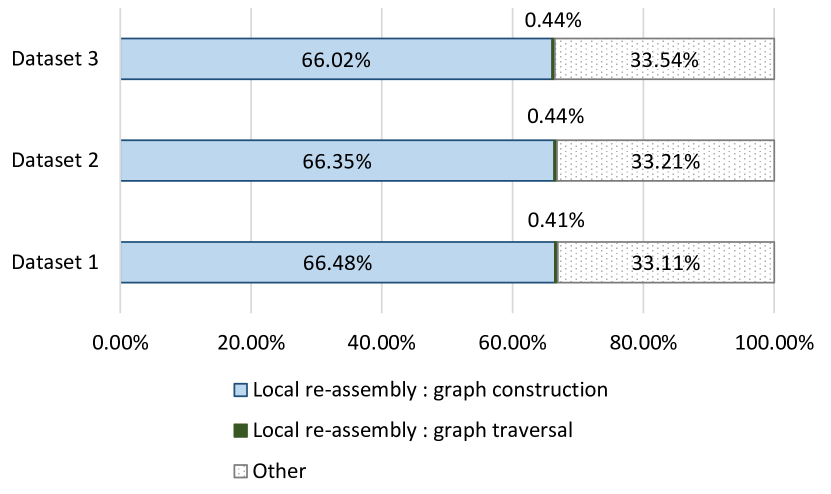
Figure 3.1: Distribution of execution time for Platypus variant caller

In this paper, we introduce several improvements to the original de-Bruijn graph-based local re-assembly algorithm such that locality in memory accesses is increased and the processor cache is utilised efficiently. One of the most efficient improvements we apply is to exploit existing alignment information in the graph construction process. Our proposed improvements result in the algorithm being about twice as fast as the original algorithm. In order to test the proposed algorithm, we ported it into the Platypus variant caller. The modified Platypus implementation is available at [159].

The rest of the paper is organized as follows. Section 3.2 discusses related work. Then in Section 3.3 we explain the de-bruijn based local assembly algorithm. Then in Section 3.4 we present our optimization techniques. Next, in Section 3.5 we present the experimental setup and results. After that, Section 3.6 elaborates the future directions. Finally, we conclude in Section 3.7.

3.2 Background of deBruijn Graph based Local Re-assembly

Modern variant callers such as GATK HaplotypeCaller [80] and Platypus[84], consist of local re-assembly, reads to haplotypes alignment and variant identification. In the GATK Haplotypecaller, aligning reads to the haplotypes (using the Pair-HMM algorithm) takes much of the processing time [144]. However, by the use of Intel’s Advanced Vector Extension (AVX) instructions and FPGAs, this processing time can be considerably reduced (by 720X using Intel AVX and 3,857X using FPGA [160]). The latest versions of GATK HaplotypeCaller support Intel AVX and FPGA [161] (the latter as an experimental feature). Furthermore, tools such as Avacado [162] consist of algorithms with lower time complexity for aligning reads to haplotypes. Platypus is a newer variant caller which is faster, with better indel accuracy than the widely used GATK HaplotypeCaller [163, 84]. Platypus aligns reads to haplotypes using a Single Instruction Multiple Data (SIMD) accelerated Needleman-Wunch algorithm. Hence the alignment phase is already fast. However, as discussed above more than 60% of the time of Platypus is spent on de Bruijn graph-based local re-assembly.

De Bruijn graphs were first used for de novo assembly, where assembling is done solely using the reads when a reference genome is unavailable. Several researchers have proposed techniques for de Bruijn graph optimisation, for de novo assembly, where the inputs to the assembler are unaligned reads. However, in the case of aligned reads for local re-assembly, the utility of the optimisations used for de novo assembly are limited. The graph for local re-assembly is much smaller: only a few megabytes for local re-assembly compared to several gigabytes for de novo assembly. This is because the whole genome is considered at once for de novo assembly, whereas the local assembly is performed in small regions (For instance a region is 1500 bases in Platypus). Consequently, optimisation techniques for de novo assembly have focused on processing large graphs through memory size optimisation or parallelising. Work such as Cortex [112], SOAPdenovo2 [164] and [165] have compressed the graph in size, while ABySS [110] and [166] have parallelised the graph across clusters. However, as the graph is small for local re-assembly, techniques used for large graphs are superfluous.

In summary, the present bottleneck in modern variant callers is the local re-assembly process. To the best of our knowledge no one has focused upon optimizing de Bruijn graph-based local re-assembly by utilising the information from aligned reads for superior cache usage.

3.3 Baseline Algorithm

In local re-assembly, the reference and the reads are used to construct a de Bruijn graph. Typically, a region of several thousands of bases is considered at a time. The reference and the reads are broken into k-mers, such that adjacent k-mers overlap by k-1 bases (see example in Fig. 3.2 and Fig. 3.3). Each unique k-mer forms a node in the graph, and the edges of the graph link adjacent k-mers.

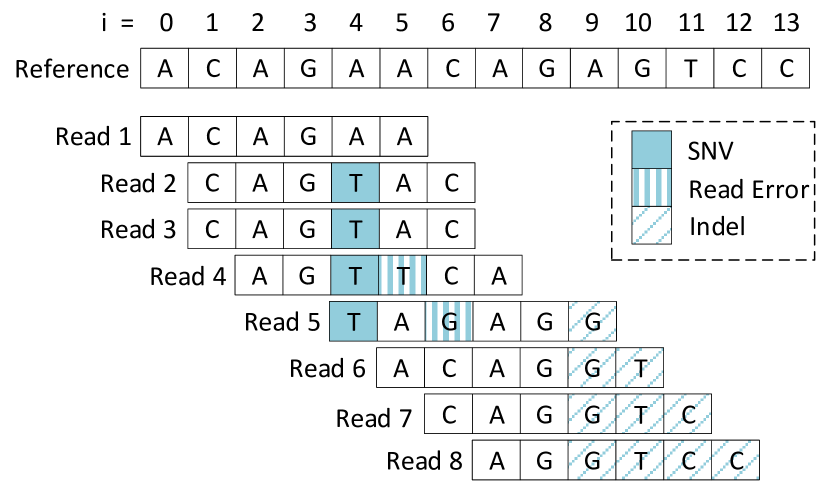
Figure 3.2: A region of the reference and few mapped reads

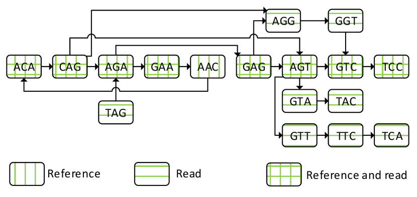
Figure 3.3: De Bruijn graph for the region

This section gives a brief account of a typical de Bruijn graph construction algorithm for local re-assembly. The example region of the reference, and the mapped reads to the region in Fig. 3.2 and its de Bruijn graph in Fig. 3.3 will be used throughout the algorithm explanation. In this simplified example, the read size and the k-mer size are 6 and 3 respectively (this is for demonstration purpose only and in reality, they are around 100 and 15 respectively). Bases corresponding to a probable single nucleotide variant (SNV), read errors and an indel are shaded as per the legend in Fig. 3.2. The de Bruijn graph in Fig. 3.3 is constructed out of all the k-mers in the region in Fig. 3.2. Nodes can be either shared by both reference and reads or belong to only one, as shown in Fig. 3.3. In addition note that a node for a certain k-mer is unique, despite the number of occurrences of the k-mer in the reference or reads. The graph is typically stored in computer memory using dynamically allocated nodes where memory pointers represent the edges.

A hash table data structure is required so that repeated accesses to the same node can locate this node quickly for performance reasons during construction of the graph. As an example, consider the ‘CAG’ k-mer in Fig. 3.3 which is shared by both reference and reads. Fig. 3.2 shows that ‘CAG’ is repeated twice in the reference and five times in the reads. During graph construction, a node will be created at the first occurrence, but it must be found within the created graph for each subsequent occurrence. Instead of exhaustively searching all nodes, the hash table is used for fast search. A hash table for the example in Fig. 3.3 is shown in Fig. 3.4. The index of the hash table for a particular k-mer is found by applying a hash function to the k-mer. The simple hash function used in this example is the addition of the ASCII values of the characters in the k-mer, subjected to the modulo operator of the number of hash table entries. For instance, there are 8 entries in the hash table and the index for the k-mer ‘ACA’ can be found by (‘A’+‘C’+‘A’)%8 which is 5. Hence The address to the node containing ‘ACA’ is in index 5 in Fig. 3.4 as denoted by ‘*ACA’.

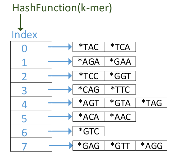
Figure 3.4: The hash table

Algorithm 1 and Algorithm 2 show how the graph is constructed. Note that these algorithms are not full implementations, but are the necessary components to explain our methodology. Algorithm 1 shows how the reference is loaded to the de Bruijn graph. Algorithm 2 illustrates how reads are then loaded to the same graph.

In Algorithm 1, reference is an array that contains the reference genome. The algorithm iterates through the reference while adding edges between adjacent k-mers. For the example in Fig. 3.2 and Fig. 3.3, the algorithm will add edges in the order, ACA-CAG, CAG-AGA, AGA-GAA etc.

Algorithm 1 Load the reference to de Bruijn Graph

1:function loadReference(reference)

2:     for i = 0 : (region_size - kmer_size) do

3:         kmer1$\leftarrow$ reference[i : i+kmer_size]

4:         kmer2$\leftarrow$ reference[i+1 : i+1+kmer_size]

5:         addEdge(kmer1,kmer2)

6:     end for

7:end function

In Algorithm 2, readsInWindow is a buffer consisting of all the mapped reads in the region sorted using the mapped position. For each read, edges are added between adjacent k-mers. In our example, ACAGAA is the first read. Edges are added in the order ACA-CAG, CAG-AGA, AGA-GAA for this read. Similarly, all other reads will be processed.

Algorithm 2 Load reads to de Bruijn Graph

1:function loadReads(readsInWindow)

2:     for read in readsInWindow do

3:         for i = 0 : (read_length-kmer_size) do

4:              kmer1 $\leftarrow$ read[i : i+kmer_size]

5:              kmer2 $\leftarrow$ read[i+1 : i+1+kmer_size]

6:              addEdge(kmer1,kmer2)

7:         end for

8:     end for

9:end function

Algorithm 3 shows the implementation of addEdge function used in Algorithms 1 and 2. The hashTableLookUpOrInsert function in Algorithm 3 locates the corresponding node for a given k-mer, using the hash table. If no memory pointer exists in the hash table for a node containing the k-mer, then memory is allocated for a new node and the hash table is updated. Finally, hashTableLookUpOrInsert returns the memory pointer to the node. The addEdge function calls hashTableLookUpOrInsert on both kmer1 and kmer2. Finally, createLink actually adds the connection between the nodes by storing the pointer to the second node ptr2 in the first node.

Algorithm 3 Add an edge connecting kmer1 and kmer2

1:function addEdge(kmer1,kmer2)

2:     ptr1 $\leftarrow$ hashTableLookUpOrInsert(kmer1)

3:     ptr2 $\leftarrow$ hashTableLookUpOrInsert(kmer2)

4:     createLink(ptr1,ptr2)

5:end function

3.4 Methodology

In this section, We show how the algorithms in Section 3.3 are modified to minimise accesses to the RAM. First, we give a simplified overview of our methodology. Then, we present additional technical information so that our method can be replicated in any de Bruijn graph-based variant caller.

3.4.1 Simplified Overview

The hash table produced during graph construction (explained in Section 3.3) is too large to totally reside in cache. Hence it must reside in RAM. Accesses to a hash table are random accesses and therefore cache misses will occur very frequently. We propose techniques to minimize these random memory accesses, by exploiting the following two factors:

• The input reads to the variant caller are already aligned to the reference - The input to a variant caller is a set of reads which are already aligned to the reference. Information from the already aligned reads can be exploited for efficient utilization of the memory hierarchy, minimizing random accesses to the RAM. For instance, alignment information can be used to predict the majority of memory locations. Such predictions can minimise random accesses to the RAM.

• Variants and sequencing artefacts are rare - In cases of variants or sequencing artefacts, memory accesses will deviate from the expected pattern. For instance, predictions that bypass the hash table can be incorrect, requiring random accesses to the RAM. However, these events are very low as we show in Section 3.5.

Algorithm 1 is modified such that a cache friendly array is filled during the construction of k-mers for the reference genome. Then, Algorithm 2 is modified to utilise this filled cache friendly array, to reduce the memory accesses to the RAM. Furthermore, Algorithm 3 is introduced with an additional variable which is register-friendly. This register-friendly variable accelerates the construction of graph edges by eliminating redundant accesses to the cache and the RAM.

3.4.2 Algorithm in Depth

In Fig. 3.2, for position 1 (i=1), CAG is the k-mer in the reference as well as the first three reads. Similarly, if there were no variants (such as SNV, Indel) or read errors, the k-mer in the reference and the reads should be the same for each position. However, variants and read errors cause k-mers in the reads to differ from that of the reference. For instance, the k-mers (at position 4) for the second to fifth reads are TAC, TAC, TTC and TAG while the k-mer on the reference for that particular position is AAC. This difference is due to the SNV at position 4 and the read errors at positions 5 and 6 in the fourth and fifth reads. However, variants and read errors are less frequent. Variation between a particular human genome and the reference human genome is about 0.5% [12], and the read errors in modern sequencing machines are about 0.1% - 1% [51]. Thus, in about 99% of the time, the k-mers in the reads would be identical to the k-mers in the reference at a particular position. This high probability can be used to predict the memory addresses of nodes, minimizing accesses to the hash table. This is accomplished by a pointer array referred to as the nodeCache (see Fig. 3.5), which is populated when loading the reference to the graph.

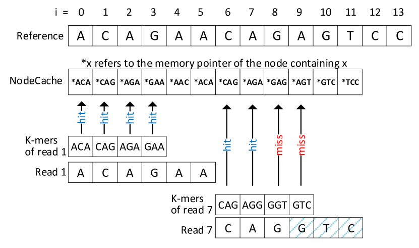
Figure 3.5: Elaboration of how mapping information is used for improving cache performance

Fig. 3.5 elaborates on how the nodeCache is used. The reference and the two reads in Fig. 3.5 used for illustration are taken from Fig. 3.2. The nodeCache in Fig. 3.5 has been populated when loading the reference to the graph, by storing the node address that corresponds to position i. For instance, position 0 on the reference forms the k-mer ACA and the memory address for the node containing this k-mer is stored at index 0 of the nodeCache. This nodeCache is utilised when loading the reads to the graph. Consider the read ACAGAA and its k-mers in Fig. 3.5. This read is mapped to position 0 on the reference and hence the four k-mers ACA, CAG, AGA and GAA map to positions 0, 1, 2 and 3 respectively. When loading these k-mers to the graph, the corresponding location in the nodeCache is looked up as shown using arrows in Fig. 3.5. As this read is exactly the same as the reference, all the accesses are hits to the nodeCache. However, in the other read on Fig. 3.5, two misses have occurred due to the marked indel on the read. As explained earlier, variants and read errors are less frequent and therefore, the misses are fewer. In the case of a hit to the nodeCache, the node can be directly accessed. The hash table has to be accessed only in case of a miss to the nodeCache. If the nodeCache was not used then all these accesses would have to go through the hash table, and thus access memory randomly.

Although this nodeCache is an array originally residing in the memory, it is cache friendly due to the spatial and temporal locality of accesses to the array. For instance, in Fig. 3.5, observe how the accesses to the nodeCache (marked using arrows) for consecutive k-mers in a read exhibit spatial locality. Temporal locality is observed for accesses to the NodeCache due to consecutive reads. In Fig. 3.2 note how consecutive reads overlap to each other. Hence, locations in the nodeCache corresponding to a read are re-accessed for the next read, exhibiting temporal locality. For instance, the k-mer CAG which is accessed for the first read ACAGAA has to be accessed again when processing the second read CAGTAC. Due to both this spatial and temporal locality among accesses, the nodeCache array is cache friendly.

In addition to the above, the end node of an edge will always be the start node of the next edge, throughout the read. For instance, the edges will be added in the following order: 1. ACA-CAG; 2. CAG-AGA; and 3. AGA-GAA for the read ACAGAA. Note how CAG and AGA which are the end nodes for edges 1 and 2, are the starting nodes for edges 2 and 3, which causes repeated accesses to memory locations. This pattern is observed for the reference as well. Though these accesses are already cache friendly due to the temporal locality, they can be made even faster by using a register (which we refer to as lastAccess). This lastAccess register is used to store the memory pointer to the end node of the current edge, to be used when loading the start node of the next edge. In an implementation for a general purpose processor, lastAccess can be a globally declared variable

Implementation for the method above is given in Algorithm 4 and Algorithm 5. Algorithm 4 shows how the reference is loaded to the de Bruijn graph. A globally accessible variable lastAccess is used for storing the end node of each edge (line 1 of Algorithm 4). A globally accessible array nodeCache is initialized with NULL pointers (line 2 of Algorithm 4). The k-mers are extracted from the reference as previously. Function addEdge called at line 7 of Algorithm 4 now returns the pointer (ptr1) to kmer1 which is then stored in the nodeCache (at line 8 of Algorithm 4).

Algorithm 4 Load the reference to de Bruijn Graph

1:global lastAccess = NULL

2:global nodeCache[region_size] = {NULL}

3:function loadReference(reference)

4:     for i = 0 : (region_size-kmer_size) do

5:         kmer1 $\leftarrow$ reference[i : i+kmer_size]

6:         kmer2 $\leftarrow$ reference[i+1 : i+1+kmer_size]

7:         ptr1 $\leftarrow$ addEdge(kmer1,kmer2,i,i+1)

8:         nodeCache[i] $\leftarrow$ ptr1

9:     end for

10:end function

Algorithm 5 shows how reads are loaded. Function getMappedPosition at line 3 retrieves the position on the reference to which the read is mapped. The positions of the k-mers are then computed and provided as arguments to addEdge (line 7-9 of Algorithm 5).

Algorithm 5 Load reads to de Bruijn Graph

1:function loadReads(readsInWindow)

2:     for read in readsInWindow do

3:         readMapping = getMappedPosition(read)

4:         for i = 0 : (read_length-kmer_size) do

5:              kmer1 $\leftarrow$ read[i : i+kmer_size]

6:              kmer2 $\leftarrow$ read[i+1 : i+1+kmer_size]

7:              pos1 $\leftarrow$ readMapping+i

8:              pos2 $\leftarrow$ readMapping+i+1

9:              addEdge(kmer1,kmer2,pos1,pos2)

10:         end for

11:     end for

12:end function

Algorithm 6 elaborates the addEdge function. First, kmer1 (which is the start node of the current edge) is compared with the k-mer in lastAccess at line 2 of Algorithm 6. If identical, there is no requirement to inspect the NodeCache or hash table. Otherwise, LookUp will be called which will inspect the NodeCache at line 5 of Algorithm 6. Unlike kmer1, the end node of the edge kmer2 is directly checked in the NodeCache by calling LookUp at line 7 of Algorithm 6. Finally, the end node of the current edge is backed up on lastAccess for future use and createLink is called (line 8-9 of Algorithm 6). createLink is same as described previously in Section 3.3.

Algorithm 6 Add an edge connecting kmer1 and kmer2

1:function addEdge(kmer1,kmer2,pos1,pos2)

2:     if lastAccess!=NULL and lastAccess.kmer==kmer1 then

3:         ptr1 $\leftarrow$ lastAccess

4:     else

5:         ptr1 $\leftarrow$ LookUp(kmer1,pos1)

6:     end if

7:     ptr2 $\leftarrow$ LookUp(kmer2,pos2)

8:     lastAccess $\leftarrow$ ptr2

9:     createLink(ptr1,ptr2)

10:     return ptr1

11:end function

The function LookUp in Algorithm 7 which is called at lines 5 and 7 of Algorithm 6, attempts to locate the node for the k-mer in the nodeCache. If it is a hit to the nodeCache, the pointer to the node can be immediately returned (line 3-4 of Algorithm 7). The hash table is accessed only in case of a miss (line 6 of Algorithm 7).

Algorithm 7 First lookup in the nodeCache and then in hash table

1:function LookUp(kmer,pos)

2:     cacheItem = nodeCache[pos]

3:     if cacheItem!=NULL and cacheItem.kmer==kmer then

4:         ptr $\leftarrow$ cacheItem

5:     else

6:         ptr $\leftarrow$ hashTableLookUpOrInsert(kmer)

7:     end if

8:     return ptr

9:end function

Fig. 3.6 summarises how memory accesses are allocated. A memory access to lookup the memory address of a node in the graph corresponds either to a start node or an end node of an edge in the graph (as explained previously). If the access is for a start node, the lastAccess register will be inspected as shown in Fig. 3.6. If a hit occurs when looking up the lastAccess register, the lookup process completes at the cost of only reading that register. In case of a miss to the lastAccess register, the node will be looked up in the nodeCache as shown in the figure. In case of a hit to the nodeCache, the process ends there, at the cost of accessing cache memory. In case of a miss to the nodeCache, the hash table has to be accessed as shown. The cost of accessing the hash table residing in the RAM is high, but misses that end up in the hash table are rare (as mentioned previously). For end nodes, the inspection starts directly from the nodeCache as shown in Fig. 3.6. In summary, if not for the lastAccess register and the nodeCache all the accesses would directly go to the hash table causing frequent accesses to RAM.

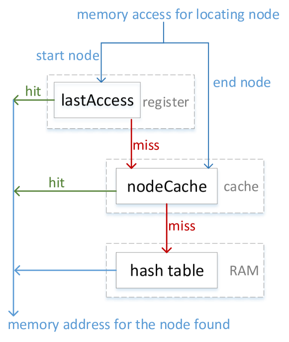
Figure 3.6: Summary of the outcome of the proposed method

3.5 Results

All experiments were performed on a server with four Intel Xeon X7560 processors (total of 32 cores / 64 CPU threads and 256 GB of RAM). The Platypus variant caller (downloaded from [167]) that implements the algorithm in Section 3.3 is referred to as the baseline implementation. The modified version of Platypus based on the method in Section 3.4 is referred to as the optimised implementation. Three real datasets from the 1000 genomes project (same whole genome sequencing data used in [84] for performance assessment of Platypus, downloaded from [168]) were used for experiments. The three datasets are aligned 75-86 X 100-bp paired-end Illumina HiSeq 2000 reads (BAM files) for the parent-offspring trio NA12878, NA12891 and NA12892. Platypus was run using the default parameters with de Bruijn based assembly turned on. Variants were called on all chromosomes including X and Y.

Section 3.4 described how accesses to the hash table are minimised by using a register that stores the previous node (referred as lastAccess) and a cache friendly array (referred as NodeCache). Fig. 3.7 shows how memory accesses to lastAccess, nodeCache and the hash table are distributed. The X-axis in Fig. 3.7 denotes the dataset and the type of memory access. Y-axis shows the access percentage for each item on the X-axis. The data used to compute the percentages in Fig. 3.7 are given in Table 3.1. These data in the table were obtained by running the optimised implementation with software counters introduced to count different memory accesses. The first column of Table 3.1 is the dataset and the second column is the memory access type. The third column contains the number of memory accesses occurred when locating start nodes of the edges in the de Bruijn graph. Similarly, the fourth column is for end nodes. The last column is the total number of accesses which is the sum of columns three and four. Note that the numbers are given in x10⁹. The number of hits to the lastAccess register is equal to the number of times the program reaches line 3 in Algorithm 6. Only the accesses to start nodes are responsible for lastAccess hits. Therefore, lastAccess hits due to end nodes are 0 as shown in the Table. Similarly, Nodecache accesses and hash table accesses map to lines 4 and 6 respectively in Algorithm 7. The function LookUp in Algorithm 7 called at line 5 of Algorithm 6 corresponds to start nodes. Similarly, LookUp called at line 7 of Algorithm 6 corresponds to end nodes. The data in Table 3.1 includes accesses occurred when loading both the reference and the reads to the de Bruijn graph. The percentage value for each item in Fig. 3.7 is calculated out of the total memory accesses for that data set. For instance, the total memory accesses for dataset NA12878 is the sum of the three values 317.36,301.35 and 25.66 in the last column of Table 3.1. The values 317.36, 4.71, 296.64, 0.11 and 25.55 for dataset NA12878 when expressed as a percentage of the above sum equates the percentages 49.25%,0.73%, 46.04%, 0.02% and 3.96% respectively in Fig. 3.7.

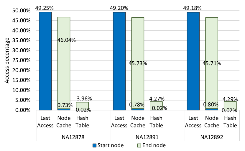
Figure 3.7: Distribution of memory accesses in the optimised implementation

Table 3.1: Memory access distribution in the optimised implementation

Dataset	Memory access type	Start nodes ($\times$109)	End nodes ($\times$109)	Total ($\times$109)
NA12878	Last Access	317.36	000.00	317.36
	Node Cache	004.71	296.64	301.35
	Hash Table	000.11	025.55	025.66
NA12891	Last Access	288.57	000.00	288.57
	Node Cache	004.59	268.26	272.85
	Hash Table	000.11	025.02	025.13
NA12892	Last Access	284.67	000.00	284.67
	Node Cache	004.61	264.54	269.15
	Hash Table	000.11	024.86	024.97

In Fig. 3.7, observe that for all datasets about 49% of total accesses are hits to the lastAccess register. Note that all hits to lastAccess are for start nodes. Then about 46.5% of accesses are hits to the nodeCache. The majority are from end nodes, as most of the start nodes have already been resolved through the lastAccess register. Observe that only about 4.5% of the accesses must go to the hash table. The implications of this figure are that only 4.5% of the accesses are misses to the RAM and therefore the techniques presented in Section 3.4 have enabled efficient usage of the memory hierarchy. However, 4.5% is higher than the percentage anticipated in Section 3.4 mainly because the values in Fig. 3.7 also include the memory accesses when loading the reference to the graph. Additionally, alignment artefacts would cause mismatches between k-mers in reference and reads, which in turn would also have increased the percentage.

Fig. 3.8 compares the time taken for graph construction by the baseline implementation and the optimised implementation. For each dataset, each implementation was run using 8, 16, 32 and 64 threads, which are shown as 8t, 16t, 32t and 64t along the X-axis. The Y-axis shows the runtime for graph construction for each case, in seconds. In all cases, the optimised implementation was at least twice as fast as the baseline implementation. Since the execution times for Platypus is considerable for the three large datasets used, the execution times given in Fig. 3.8 are an average of three repetitions. All three repetitions consistently produced values which were significantly similar on a general-purpose server (Supplementary Table S1). To further validate the claims on the speed-up, we performed two experiments with small datasets so that each test can be repeated a large number of times, with the intention to test the following: 1. the variability of the execution time for the same dataset (randomness due to the operating system scheduling); and 2. the variability in the speedup for different datasets.

In the first experiment we repeatedly ran the baseline implementation and the optimised implementation for a single data set 100 times for each implementation (Supplementary Table S2). Only the chromosome 1 of the NA12878 dataset is considered and executed with 64 threads for 100 repetitions. The two distributions (baseline implementation and optimised implementation) are near normal (Supplementary Figure S1 and S2 - the two outliers are explained in the figures). We performed an independent random sample t-test on log-transformed data to test the null hypothesis that the data in the two distributions come from populations with equal means. The log-transformed values were preferred, as the exponent of the difference between two means provides the speed-up. The mean speed-up was 2.047, with a 95% confidence interval of 2.042-2.053. The null hypothesis could be rejected at the 5% significance level with a p-value <0.0001. Hence, we may conclude that the observed speed-up is not due to random variations.

In the second experiment we executed the baseline implementation and the optimised implementation on 69 different datasets (Supplementary Table S3). Each chromosome (chr 1-22 and chr X) of the three datasets NA12878, NA12891 and NA12892 were considered as a separate dataset (thus the 69 different datasets). A paired sample t-test was performed on the log-transformed data (X - log transformed times for baseline implementation and Y - log transformed times for optimised implementation) to test the null hypothesis that the mean of X-Y is equal to 0 (speed-up is 1). The distribution of X-Y was near normal (Supplementary Figure S3). The mean speed-up was 2.028, with a 95% confidence interval of 2.017-2.039. The null hypothesis could be rejected at the 5% significance level with a p-value <0.0001. Hence, the speed-up is evident across different datasets.

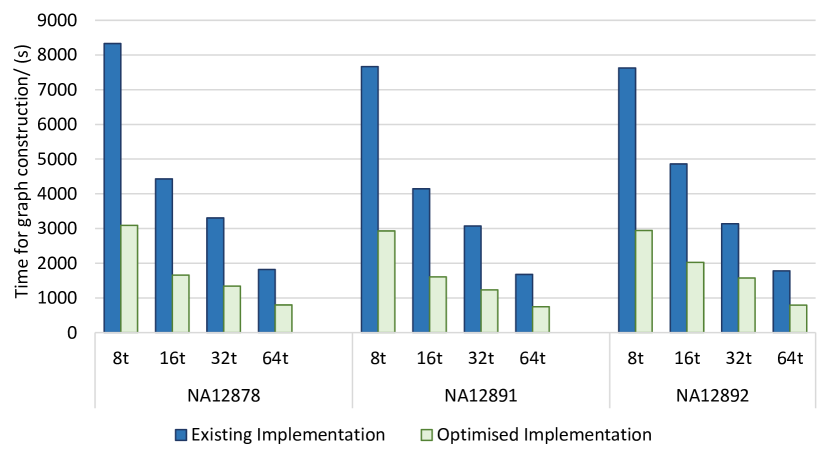
Figure 3.8: Execution time for the baseline implementation and the modified implementation

3.6 Discussion

According to profiling done on the baseline implementation, approximately about:

1. 70% of the memory accesses to the RAM (during graph construction) are due to the hash table, and

2. 30% are other memory accesses not due to the hash table.

Our optimisation technique reduced only (a) memory accesses. The speed up for the whole graph construction process was about 2X. However, note that this speed up was obtained purely by modifying the algorithm that runs on a general purpose processor. On general purpose processors, the programmer’s control of the caches and the registers is limited. Hence, nodeCache is implemented as an array that originally resides in the RAM, and lastAccess is implemented as a global variable. In contrast, it is possible to have an exclusive cache for the nodeCache and an exclusive register for lastAccess when building a custom processor. Therefore, the proposed algorithm opens the door to building custom processors such as Application Specific Instruction Set Processors (ASIP), where the baseline algorithm is not suitable. In such a case, the observed speed up would be higher. Furthermore, the proposed algorithm can lead to efficient local re-assembly implementations for any other system having a memory hierarchy such as Graphics Processing Units (GPU) and Field Programmable Gate Arrays (FPGA),

RAM accesses in (b) are due to other memory accesses that occur during graph construction, such as,

1. reading the reference genome in Algorithm 1 (line 3 and 4) ,

2. reading the reads in Algorithm 2 (line 4 and 5) , and

3. writing to the located nodes to add connection between k-mers inside createLink function (called at line 4 of in Algorithm 3)

Out of these, 1 and 2 are already cache friendly due to the spatial locality of access. Accesses to the RAM are still caused when refilling cache lines. In contrast, 3 is not cache friendly due to the large size of the data structure that stores a node. A node contains space for fields such as memory pointers to adjacent nodes and the total node size is even larger than the size of a cache line of a general purpose processor. For instance, the typical cache line size of a CPU is 64 bytes and the size of a node in Platypus is 65 bytes. Hence at least one access to the RAM is required for each node access to fill a cache line. A large cache line size that fits several nodes to one cache line can be implemented during custom processor construction. In addition, strategies such as cache pre-fetching (fetching the next adjacent cache line from the RAM before it is actually required) would be helpful to boost the performance.

3.7 Summary

The de Bruijn graph construction during the local re-assembly step of modern variant callers consumes more than 60% of the total variant calling time. We have shown how the existing algorithm can be modified such that the locality of memory accesses are improved, which in turn improves the efficient usage of faster cache memories. The results show that these changes improve the performance of de Bruijn graph construction by a factor of around two when implemented on a general purpose processor. The modified algorithm opens the door to much higher acceleration of local re-assembly on GPU, FPGA and ASIP. The implementation of the algorithm which is integrated into the Platypus Variant Caller is publicly available at [159].

Chapter 4 Featherweight Long Read Alignment using Partitioned Reference Indexes

  This chapter is published in Nature Scientific Reports under Creative Commons CC BY license at H. Gamaarachchi, S. Parameswaran, and M. A. Smith, “Featherweight long read alignment using partitioned reference indexes,” Scientific Reports 9, 4318 (2019). DOI: https://doi.org/10.1038/s41598-019-40739-8 [25]
 

The advent of Nanopore sequencing has realised portable genomic research and applications. However, state of the art long read aligners and large reference genomes are not compatible with most mobile computing devices due to their high memory requirements. We show how memory requirements can be reduced through parameter optimisation and reference genome partitioning, but highlight the associated limitations and caveats of these approaches. We then demonstrate how these issues can be overcome through an appropriate merging technique. We incorporated multi-index merging into the Minimap2 aligner and demonstrate that long read alignment to the human genome can be performed on a system with 2GB RAM with negligible impact on accuracy.

4.1 Introduction

Long read sequencing has revolutionised genome research by facilitating the characterisation of large structural variations, repetitive regions, and de-novo assembly of whole genomes. Pacific Biosciences (PacBio) and Oxford Nanopore Technologies (ONT) are leading manufacturers that produce long read sequencers. In particular, ONT manufacture sequencers smaller than the size of a mobile phone that can nevertheless output more than 1TB of data in 48 hours. Such highly portable sequencers have realised the possibility of performing genome sequencing in the field. For instance, ONT’s MinION sequencer has been used for Ebola virus surveillance in Guinea [16], mobile Zika virus surveillance in Brazil [17], and for experiments on the International space station [19].

The advent of highly portable DNA sequencers raise the need for local data processing on devices such as mobile phones, tablets and laptops. Facilitating genomic data analysis on mobile devices avoids the need for high speed internet connections and enables real-time genomic tests and experiments. For Nanopore sequencers, a pico-ampere ionic current signal is produced for each DNA read, which is subsequently converted to nucleotide bases via applied machine learning models. Until recently, a high performance workstation (Quad-core i7 or Xeon processor, 16GB RAM, 1TB SSD) was required for live base calling, the process of converting ionic signal to nucleotide sequences.

Most genomic analyses depend on base calling as an initial step, which can be efficiently performed through GPGPU software implementations on graphics cards or, quite conveniently, on dedicated portable hardware (ONT manufacture one such device, termed ‘MinIT’). Next, base called reads are typically aligned/mapped to a reference, in case of reference guided assembly, or aligned to themselves in case of de-novo assembly. Subsequent analyses (i.e. consensus sequence generation, variant calling, methylation detection, etc) should follow this alignment step. Therefore, an alignment tool that can run on portable devices such as mobile phones, tablets and laptops is the next step in realising the full portability of the whole Nanopore processing pipeline.

Minimap2 [101] is a general purpose mapper/aligner that is compatible with both DNA and RNA sequences. Minimap2 can align both long reads and short reads, either to a reference or an assembly contig. Minimap2 first employs hashing followed by chaining for coarse grain alignment. Then it performs an optional base level alignment using an optimised implementation of the Suzuki-Kasahara DP formulation [102]. Minimap2 stands out as the current aligner of choice for long reads, among other long read aligners such as BLASR [96], GraphMap [97], Kart [98], NGMLR [99] and LAMSA [100]; not only is it  30 times faster than existing long read aligners, but its accuracy is on par or superior to other algorithms [101]. Hash table based approach in Minimap2 has shown to be effective against long reads. In contrast, FM-index [67] based short read aligners such as BWA [70] and Bowtie [68] have shown to fail with ultra long reads (i.e. several hundred kilobases or more) [56].

Most alignment tools build an index of reference sequences that is stored in volatile memory. Whilst this is manageable for small genomes such as individual bacteria ($\mathtt{\sim}$5Mb), fungi ($\mathtt{\sim}$50Mb) or insects ($\mathtt{\sim}$400Mb), most vertebrates and some plant species require large amounts of memory, as their genomes are in the 1-100 Gb range. For example, building an index for the GRCh38 human genome reference requires over 11.2GB of volatile memory, and at the very least 8.8GB to map nanopore reads to a pre-computed index with Minimap2.

To accelerate the development and uptake of real-time genomic applications in field research and point of care medical testing, long read sequence alignment should be performed on ultra-portable computing devices. These can include mobile phones, microcomputer boards, Field-Programmable Gate Arrays (FPGAs), and other embedded systems, such as ONT’s “MinIT” and “Mk1c MinION” devices. Such hardware rarely have more than 4GB of RAM, therefore more expensive and less portable equipment is typically required for sequence alignment (high-end laptops, internet connectivity, power generation, etc).

Here, we describe strategies for long read alignment to large reference genomes (or collections of genomes) using low amounts of memory. We present an efficient approach to achieve this by splitting a genome index into smaller partitions. Although partitioned indexes are not a novel concept [169, 170, 151], we expose the caveats of their use on the accuracy of entailing alignments. We present a solution to these issues by merging multi-part alignments via serialisation of internal data structures of the Minimap2 aligner, and demonstrate how this strategy produces alignments that are almost indiscernible from a classical single index using simulated long reads, Nanopore NA12878 reference human genome sequencing data, and a 470kb long chromothriptic read from a human cancer cell line.

4.2 Results

4.2.1 Effect of parameters on memory usage

With default options, Minimap2 requires more than 11GB of memory to create an index from the human reference genome sequence and align Nanopore reads against it (Table 4.1). Although the pre-calculated index can be saved to disk, 7.7GB are nonetheless required to subsequently load the index into memory, and between 8.8 and 11.3GB are required when intermediate data structures during alignment are included. This exceeds the average RAM capacities of high-end mobile phones and mid-range laptops. Hence, running Minimap2 on human data with default options on a typical laptop with 8GB memory or a typical mobile phone with 2GB of memory is not feasible.

Table 4.1: Memory usage of Minimap2 for default parameters

	PacBio	Oxford nanopore
Index construction	8.67 GB	11.32 GB
Index residence	6.33 GB	7.71 GB
Mapping with base-level alignment (SAM output)	8.56 GB	11.30 GB
Mapping without base-level alignment (PAF output)	7.14 GB	8.80 GB

Minimap2 was run with default parameters. Pre-set profiles map-pb and map-ont were used for PacBio and Oxford Nanopore, respectively. The peak memory usage for each event is presented. Index construction refers to the building of the index and then serialising the index to a file. Index residence is the memory required only for the index to reside in memory, such as when loading a pre-built index.

We therefore tested the relative effect of alignment parameters on peak memory usage in Minimap2 (see Materials and methods) to investigate if parameter optimisation alone can significantly reduce the memory requirements without compromising alignment quality. For this purpose, we used Sequins—synthetic DNA spike-in controls that are designed from the reverse or ‘mirrored’ human genome sequence [171]. This chirality reproduces diverse properties of the human genome, such as nucleotide frequencies, complexity, repetitiveness, somatic variation, etc. As detailed in Materials and methods, we aligned Nanopore sequencing data from Sequins to both native and reversed (not complemented) human reference genomes to compare the relative impact of Minimap2 parameters on alignment accuracy. Specifically:

• k the minimiser k-mer length (default = 15 for ONT data);

• w the minimiser window size (default = 10);

• t the number of threads (default = 4);

• K the number of query bases loaded into memory at a time (default = 500M).

Parameters k and w considerably affect the peak memory usage for holding the index in memory (Figure 4.1a). For an index without homo-polymer compression, k = 15 consumed the least amount of memory out of the values tested, as expected. In fact, the default k-mer size for ONT data in Minimap2 (pre-set command line parameter map-ont) is 15.

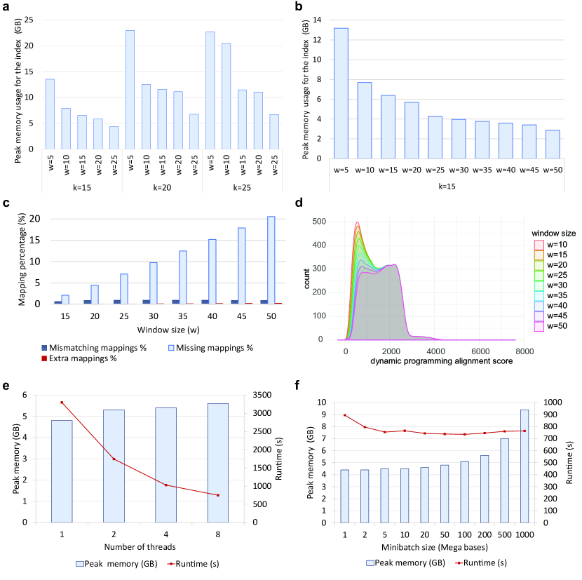
Figure 4.1: Effect of parameters on memory usage, performance and accuracy.
(a) Peak memory usage of the index for different combinations of k and w. (b) Peak memory usage of the index for a large range of w with k=15. (c) The effect of w on sensitivity and error relative to the default window size. The x-axis is the minimiser window size (w). The k-mer size is held constant at 15 for all values of w. The y-axis shows the number of missing mappings / mismatches or extra mapping (compared to the mappings from default w=10) as a percentage of the number of reads. (d) Distribution of the dynamic programming alignment score for different minimiser window sizes (w). The x-axis is the score and the y-axis is the smoothed number of mappings for a particular score. Note that the distribution is smoothed to show the trend. (e) Effect of the number of threads on memory and performance. The parameters k, w and K were held constant at 15, 25 and 200M respectively while changing the number of threads. Both the peak memory usage and the runtime were measured on a PC with an Intel i7-6700 CPU and 16GB of RAM. (f) Effect of the number of query bases loaded at a time. The parameters k, w and t were held constant at 15, 25 and 8 respectively.

Unsurprisingly, parameter w has the most prominent impact on memory usage, which decreases considerably when increasing w (Figure 4.1b). At w=50, memory usage is capped at 3GB, but the sensitivity (see Materials and methods) is substantially reduced compared to the default value of parameter w (missing mappings in Figure 4.1c). A larger w of 50 reduces sensitivity compared to the default value of w by 20%, whereas a w of 25 entails an apparent reduction in sensitivity of about 7% while nonetheless requiring more than 4GB of memory. Although sufficient for a computer with 8GB of RAM, this is still too high for smaller devices.

Importantly, the amount of mismatched mappings in mapped reads are not significantly affected by the w parameter (mismatches in Figure 4.1c), nor are the high-quality alignments as demonstrated by their dynamic programming (DP) alignment score distribution (cf. DP score > 2000 in Figure 4.1d). However, lower ($\approx$1000) DP scores are less frequent with increasing window size, as are alignments with high MAPQ scores, while those with low MAPQ scores are more prevalent (Figure 4.2). The effect of the window size is also apparent with simulated PacBio reads, where both the sensitivity and error-rate of alignments are negatively affected (Figure 4.13).

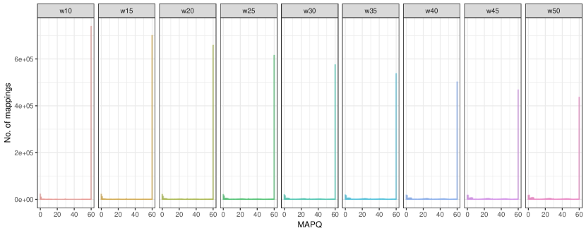
Figure 4.2: Effect of the window size parameter w on the distribution of mapping qualities (MAPQ) for synthetic spike-in controls.

The number of threads marginally increases peak memory usage (Figure 4.1e). Only about 0.8GB of additional memory was consumed when moving from 1 to 8 threads, while producing a 6-fold gain in speed. Hence, reducing the number of threads for the sake of reduced memory usage is not an efficient solution.

Intuitively, the number of query bases loaded to the memory at once (also known as the mini-batch size) heavily impacts peak memory usage. This affects the size of the internal data structures used for mapping, but does not affect the index size. Hence, this parameter does not affect alignment accuracy or the sensitivity. A lower mini-batch size reduces the peak memory usage, at the cost of reduced multi-threading efficiency (Figure 4.1f). The runtime drops when changing the mini-batch size from 1M to 5M. However, the runtime is relatively stable from a mini-batch size of 5M onwards. It is important to note that the values in Figure 4.1f are only valid for 8 threads. A large number of threads would require a large mini-batch size for optimal performance.

Although parameter adjustments (small minimiser window size value and mini-batch sizes from 5M-20M in particular) can be suitable for systems with limited RAM (for 8 CPU threads or less), tuning parameters alone cannot bring down the memory usage to a value lesser than 4GB due to a substantial loss of sensitivity. As a consequence, this inspired us to investigate the use and suitability of partitioning (or splitting) the reference sequences into distinct indexes.

4.2.2 Caveats of naive partitioned indexes

Minimap2 allows the reference index to be split by a user specified number of bases through the option I, effectively dividing a reference into smaller indexes of comparable size. This facilitates parallel computation and, in theory, enables lower peak memory requirements. However, this feature is not ideal for mapping single reads to large references, mainly because global contiguous information about the reference is unavailable. As a result, several mapping artefacts can occur, as listed below and in Figure 4.3 (N.B. these may not be as prominent when overlapping reads–the application for which index partitioning in Minimap2 was originally developed).

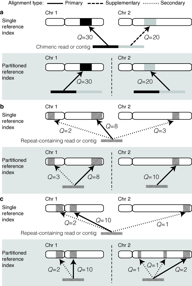
Figure 4.3: Effect of aligning sequences to single vs partitioned indexes. Uniquely mapping chimeric reads (a) can be reconstructed from a partitioned reference index with relative ease. However, sequences (or sub-sequences) that are difficult to map (i.e. low complexity regions, repetitive elements, etc) can cause artefacts when aligning to a partitioned reference index. (b) An example where one partition (chr2) contains less homologous sequences to the query sequence, producing the situation where the best alignment when using a single reference is not achieved. (c) An example where a partitioned reference introduces several additional low quality mappings that would be dismissed with a single reference index. Q: mapping quality score.

1. The mapping quality is incorrect.
   The mapping quality estimated in Minimap2 is accurate as it deliberately lowers the mapping quality for repetitive hits. However, this is not possible when only a fraction of a whole genome is present in the index (see supplementary materials of Li, H. [101]). In a partitioned index, if the same repeat lies across different partitions, the mapping quality will be overestimated (Figure 4.3b.)

2. Incorrect alignment flags.
   For a chimeric read where different sub-sequences map to different chromosomes, the supplementary mappings would be marked as primary mappings (Figure 4.3a). A repeat containing read that maps to multiple locations across different partitions will have multiple primary alignments instead of a single primary alignment (Figure 4.3b and Figure 4.3c).

3. Large output files.
   A spurious unmapped record will be printed for each partition of the index where a particular read does not map to. Furthermore, if a maximal amount of secondary alignments are specified, that number of secondary alignments would be output for each partition (Figure 4.3c). Hence, the more partitions used, the larger the output files will be. Such large outputs not only waste disk space, but they are also time consuming to parse or sort.

4. Multiple hits of the same query may not be adjacent in the output [172]
   This causes difficulties to analyse or evaluate mapping results. For instance, the Mapeval utility in Paftools (a tool bundled with Minimap2 for evaluating alignment accuracy) is not compatible with such outputs. Sorting by the read identifier would fix the issue, but requires significant computations for large files.

5. Incomplete headers in the sequence alignment/map (SAM) output
   For a partitioned index, Minimap2 suppresses the reference sequence dictionary (SQ lines) in the SAM header. Users must manually add SQ lines to the header for compatibility with downstream analysis tools.

We resolved these issues by serialising and storing the internal state of Minimap2 while mapping reads, then merging the output and processing the result a posteriori (see Materials and methods). The accuracy of this technique is discussed below.

4.2.3 Effect of using a partitioned index on alignment accuracy

We compared the alignment accuracy between a single reference index and a partitioned index, with and without merging the output. The following acronyms will be used in the subsequent text (see Materials and methods for more details):

• single-idx: Aligning reads to a single reference index;

• part-idx-no-merge: Aligning reads to a partitioned index without merging the output;

• part-idx-merged: Aligning reads to a partitioned index while applying our merging technique.

4.2.3.1 Synthetic long reads

Synthetic long reads were used as a ground truth for the evaluation of alignment accuracy (see Materials and methods). The accuracy of part-idx-merged is similar to single-idx, despite employing significantly more partitions (Figure 4.4a and 4.4b) as exemplified by the overlap of their respective curves.

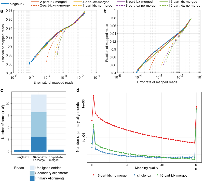
Figure 4.4: Effect of using partitioned indexes versus a single reference index on alignment quality.
(a) Base-level and (b) locus- or block-level alignment accuracy from synthetic long reads. The x-axis shows the error rate of alignments in log scale (see Materials and methods). The y-axis shows the fraction of aligned reads out of all input reads. Each point in the plot corresponds to a mapping quality threshold that varies from 0 (top right) to 60 (bottom left). These plots are akin to precision-recall plots with the x-axis inverted. (c) and (d): Alignment statistics for Nanopore whole genome sequencing data from NA12878 [56] using a 16-part index. (c) The number of total entries (primary+secondary+unaligned) for single-idx, 16-part-idx-merged, and 16-part-idx-no-merge, in log scale. The dotted horizontal line represents the number of reads. (d) Number of primary mappings in function of Minimap2 mapping quality (log scale).

In contrast, the results of part-idx-no-merge are considerably less accurate, in particular for larger quantities of index partitions. A lower error rate is observed for part-idx-merged when compared to single-idx for the lowest mapping quality values, but this effect is marginal and is associated with low sensitivity.

4.2.3.2 For real Nanopore NA12878 reads

As no ground truth is available for biological data, we evaluated alignment accuracy by comparing the number of primary/secondary alignments and unmapped reads across single and multi-partition indexes. When using single-idx, Minimap2 outputs 12.1GB of base-level alignment data in SAM format, whereas part-idx-no-merge generates much larger output (180GB). However, part-idx-merged generates 12.4GB of data–proportional to the output produced with single-idx. Hence, part-idx-merged reduces disk usage by about 14-fold compared to part-idx-no-merge. Peak disk usage is also minimised in part-idx-merged as only intermediate alignments are serialised as temporary binary files. The resulting size of temporary files generated with part-idx-merged is 29.2GB, thus achieving maximal disk usage of 41.6GB, 4 times less than part-idx-no-merge. The increased output produced by part-idx-no-merge is due to redundant unmapped entries and spurious mappings (Figure 4.4c and Table 4.2).

Table 4.2: Statistics for alignment outputs for 689,781 reads from NA12878

	single-idx	16-part-idx-no-merge	16-part-idx-merged
File size (SAM file)	12.1 GB	180 GB	12.4 GB
No of SAM entries	862,427	23,749,310	969,223
No of unaligned entries	127,177	7,365,979	120,775
No of aligned entries	735,250	16,383,331	848,448
No of primary alignments	592,748	6,228,567	654,302
No of secondary alignments	142,502	10,154,764	194,146

The number of total entries (primary + secondary + unaligned) for single-idx and part-idx-merged are comparable to the number of input reads (689,781), while part-idx-no-merge generates abundant—presumably spurious—hits. Furthermore, the distribution of mapping qualities for primary alignments between part-idx-merged and single-idx are quite similar (Figure 4.4d). Interestingly, part-idx-merged produces slightly more primary alignments with lower mapping quality scores than single-idx, a likely consequence of sampling less repetitive regions in partitioned indexes. All the strategies produce almost the same amount of mappings with quality = 60. In contrast, part-idx-no-merge has a very high number of spurious mappings for mapping qualities between 0 to 59.

A more detailed comparison of 689,781 ONT reads aligned using single-idx and 16-part-idx-merged revealed the following: 120,623 (17.49%) reads were unmapped in both; 152 (0.02%) reads mapped only in single-idx; 6,554 (0.95%) reads mapped only in 16-part-idx-merged; 562,452 (81.54%) reads mapped in both. Less than 1% of all reads presented discordant mappings when using a single or a multi-part index. Of those discordant mappings, 6,423 (95.8%) overlapped regions in the human genome annotative as repeat elements or low-complexity sequences, the majority of which were satellites and ALR/Aplha repeats from centromeres (Figure 4.5 and 4.6). Furthermore, most (97.7%) of these index-specific unique alignments stem from the multi-part index, which suggests that a reduced search space can help Minimap2 map less complex sequences, presumably through more frequent recourse of the dynamic programming step in Minimap2.

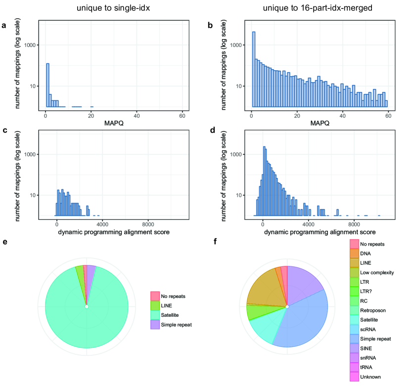
Figure 4.5: Features of alignments that were uniquely mapped in single (left column) and multiple (right column) partition indexing strategies.
(a) and (b) are the distribution of mapping quality scores (MAPQ). (c) and (d) are the distribution of dynamic programming alignment scores. (e) and (f) are the proportion of reads that map to regions of the human genome annotated as repeat elements (Repeat masker track of GRCh38 UCSC genome browser).

Figure 4.6: Genome browser screenshots of alignments unique to the 16-part index that do not overlap annotated repeats. Out of the 281 alignments only found in 16-part-idx-merged with no overlap with repeat regions, the two highest scoring alignments were found in the regions (a) chr3:185,453,170-185,456,442 and (b) chr11:14,160,389-14,161,287 respectively. The screen shots are from the Golden Helix GenomeBrowse [http://goldenhelix.com/products/GenomeBrowse]. The first track of each screen shot shows the pile-up of the alignments for the genomic region. The second track shows the repeat elements from the UCSC Repeatmasker track for GRCh38. The third track visualises the relative sequence composition of the GRCh38 reference for the particular region (A - red, C - yellow, G - green and T - blue).

Among the 562,452 reads that mapped in both single-idx and 16-part-idx-merged, 545,306 (96.95%) had the exact same primary mappings (same chromosome, strand and position). Out of the remaining 17,146 aligned reads (3.05%): 2,748 (16.02%) of mapping coordinates overlapped by at least 10% in both sets; 952 (5.55%) were classified as supplementary mappings in 16-part-idx-merged and the primary mapping in single-idx; 3,891 (22.69%) were classified as secondary mappings in 16-part-idx-merged and primary mapping in single-idx.

Of the 17,146 reads with disparate mappings, 50.5% had higher DP alignment scores for the single index, while 42.9% had higher scores in the 16-part index (Pearson’s correlation = 0.93, Figures 4.7 and 4.8). This effect was similarly observed for the MAPQ scores, with 15.2% and 12.8%, respectively, suggesting that alignments are of marginally better quality when generated with a single index. Again, these disparate mappings are largely composed of repetitive and viral sequences (Figure 4.9). when the 2,748 overlapped reads were removed from the 17,146 disparate mappings, the trend of the DP scores, MAPQs and the repeat distributions are very similar to when those are not removed (Figure 4.10).

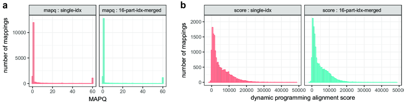
Figure 4.7: Distribution of (a) mapping quality and (b) dynamic programming alignment score for the disparate mappings (different by at least one base position) between single-idx (left) and 16-part-idx-merged (right). Disparate mappings here refer to the 17,146 aligned NA12878 reads with different primary mappings (different by at least one base position) between the two partition strategies.

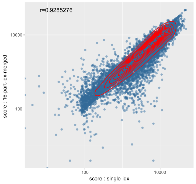
Figure 4.8: Scatter plot of alignment scores of single-idx vs 16-part-idx-merged for disparate alignments (different by at least one base position). The scatter plot contains 17,146 points representing each disparate mapping - different by at least one base position (Pearson’s correlation (r) of 0.9285). The x and y axes are in log scale. 50.5% had higher dynamic programming alignment scores for single-idx, while 42.9% had higher scores in the 16-part-idx-merged.

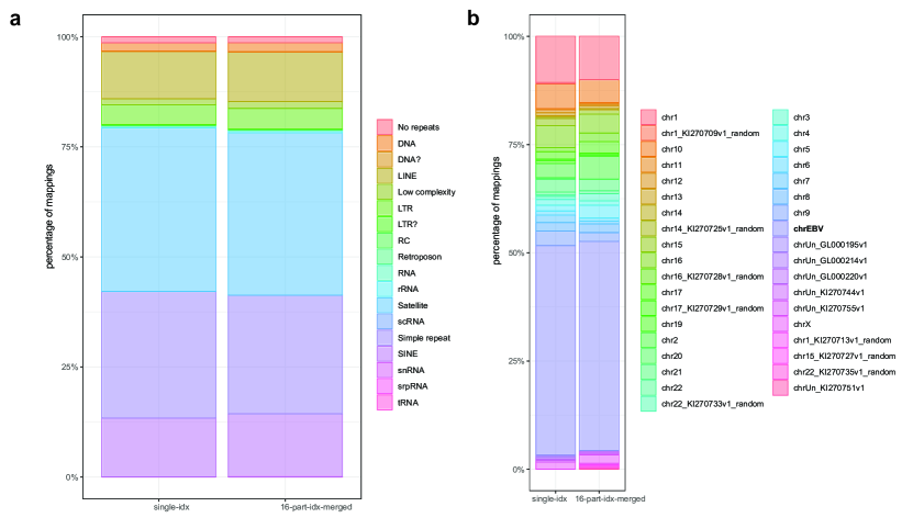
Figure 4.9: Distribution of genomic features of disparate alignments (different by at least one base position). (a) The distribution of repeat diversity in the disparate alignments (different by at least one base position) between single-idx and 16-part-idx-merged. (b) Distribution of genomic targets for the 456 (left) and 472 (right) disparate alignments (that did not overlap with annotated repeat regions) between single-idx and 16-part-idx-merged, respectively.

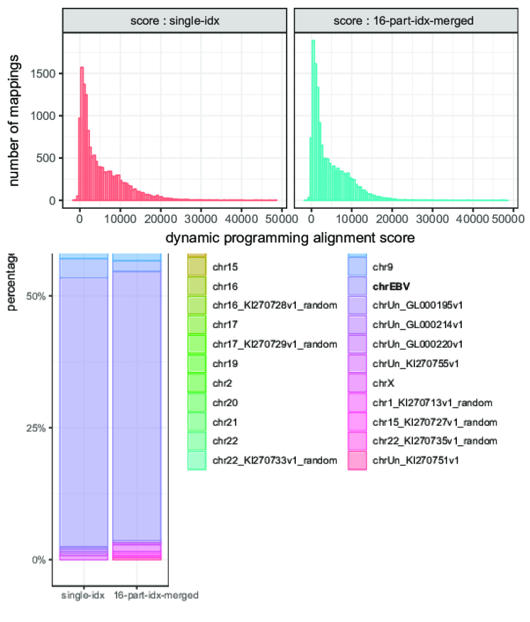
Figure 4.10: Statistics and genomic features of disparate mappings (mapping positions not overlapping at least by 10%) between single-idx and 16-part-idx-merged
Out of the 17,146 mappings that were different by at least one base position, 14,398 did not even overlap by 10% or more with their mapped locations on the reference. For those 14,398 mappings the distribution of the (a) mapping qualities and (b) alignment scores, (c) the scatter plot between the alignment scores, (d) the distribution of repeat diversity and (e) the mapping location of the mappings that did not contain repeats were almost identical to respective plots for disparate alignments –different by at least one base position.

4.2.3.3 For an ultra-long chromothriptic read

To evaluate how chimeric reads will be affected by aligning them to partitioned indexes, we tested this case on an ultra-long (473kb) chromothriptic Nanopore read from a patient-derived liposarcoma cell line [173]. Chromothripsis is a genetic phenomenon often associated with cancer and congenital diseases. It is caused by several rounds of breakage-fusion-bridge, which produce complex and localised genomic rearrangements in a relatively short segment of DNA. The single-idx produced 41 (36 primary + 5 secondary mappings) mappings (Figure 4.11a). However, part-idx-no-merge (16 partitions) produced 688 (608 primary + 80 secondary) mappings (Figure 4.11b), while mapping with part-idx-merged resulted in 47 (42 primary + 5 secondary) mappings (Figure 4.11c).

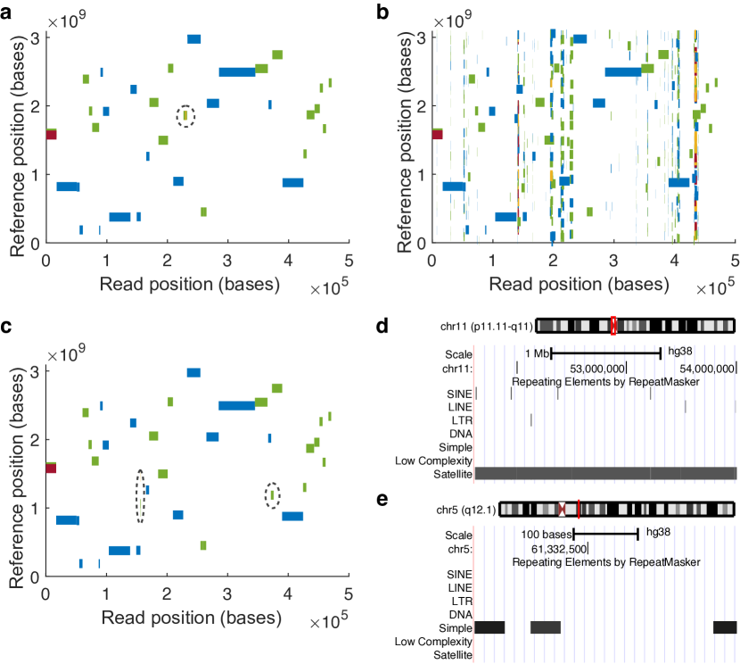
Figure 4.11: Alignment of an ultra-long Nanopore read from a chromothriptic region.
Mapping coordinates in the entire human reference genome (y-axis) in function of the position in the read, showing where sub-sequences of the chimeric read map to in the genome for (a) single-idx , (b) part-idx-no-merge , and (c) part-idx-merged. The y-axis begins with chromosome 1 at 0 and ends with chromosome X, Y, and the mitochondria at the top. The length of rectangles along the x-axis are in the correct scale to the length of the read. However, the length along the y-axis are exaggerated to a fixed value so that it is clearly visible. In (a) and (c), the areas with dotted circles contain the differences between unique mappings for each alignment strategy. Circled regions in (a) map to a genomic locus harbouring the satellite repeat displayed in (d). Out of the 6 unique mappings in (c), the segment with the highest mapping quality (6) maps to the simple repeat containing region displayed in (e).

In single-idx and part-idx-merged, 34 mappings were the same. Interestingly, there were 7 mappings unique to single-idx and 6 unique to part-idx-merged (Table 4.3). All 7 alignments unique to single-idx map to the centromeric region of the chromosome 11 (Figure 4.11d), which is composed of large arrays of repetitive DNA (also known as satellite DNA). The alignments that are unique to part-idx-merged map to simple repeats (e.g. GAGAGAGA).

Table 4.3: Mappings of the chromothriptic read which are different in single-idx and 16-part-idx-merged

The alignments which were only found in the single-idx mapped to locations in the range chr11:51616896-54006133. The ones unique to 16-part-idx-merged mapped to repetitive regions in chr5, chr6 and chr8. chr5:61332327-61332729, chr6:1610948-1611924 and chr8:60678764-60678812 contained simple repeats. chr6:125,655,477-125,659,733 had simple repeats,SINE repeats and LTR repeats

4.2.4 Memory usage and runtime of partitioned indexes

In addition to comparable quality of alignments, using a partitioned index yields impressive reductions on peak memory usage during indexing. About 7.7GB of memory is required to hold a single reference index, whereas only 1.5GB is needed for a partitioned index with 16 parts (Figure 4.12a). Peak memory usage can be further reduced by distributing or ’balancing’ chromosomes across partitions based on their size (see Materials and methods). These indexing approaches combined with a mini-batch size between 5-20 Mbases (Minimap2 parameter K) enables alignment of long reads to the human genome with less than 2GB of RAM. Although generating an index ab initio requires more memory than loading a pre-built one, this only needs to be done once for a given reference and can be performed a priori, if required.

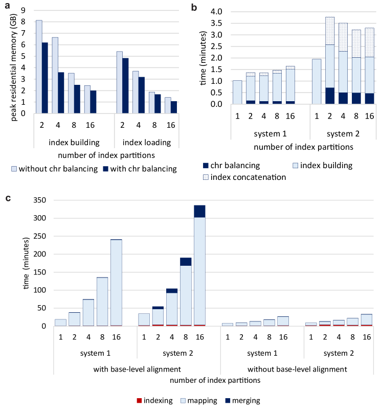
Figure 4.12: Peak memory usage and runtime for a partitioned index of the human genome. (a) Peak memory usage in function of the number of partitions for Ab initio index generation (left) and loading a pre-built index (right). Dark bars represent memory usage when performing chromosome balancing as described herein, whilst light bars represent default iterative partition distribution as implemented in Minimap2. (b) Detailed runtime metrics for index building across two computational systems. System 1 is a laptop with flash memory (Intel i7-8750H processor, 16GB of RAM and Toshiba XG5 series NVMe SSD) while system 2 is a workstation with a mechanical hard disk (Intel i7-6700 processor, 16GB of RAM and Toshiba DT01ACA series HDD). The total indexing time has been broken down into three steps; chr balancing, index building and index concatenations. Chr balancing includes the overhead for chromosome sorting, partitioning and writing each partition to a separate file. (c) Runtime for base-level alignment (left) and block/locus level mapping (right). System 1 and 2 are as described in (b). Alignment was performed on the NA12878 data (see Materials and methods) with the map-ont pre-set in Minimap2 using 8 threads. Runtime statistics are composed of indexing (index generation including the overhead), mapping (total time for aligning reads to each partition), and merging using the method described herein. Runtimes include file reading and writing.

The reduced peak memory usage of a partitioned index comes with an inherent sacrifice in computing speed. Alignment requires significantly more time than the balancing, indexing and merging steps when generating an index ab initio, which we observed to be relatively constant across different partition ranges (Figure 4.12b). Less than 10% of the total compute time (5.7h) for base-level alignment is dedicated to balancing, indexing, and merging when using mapping to 16 partitions with eight CPU threads and a mechanical hard drive. When using flash memory, the overheads have very minor impact (3% of the total compute time). Chromosome balancing, for instance, required less than 1 minute and merging required less than 2 minutes.

We observed that the alignment time increased less than linearly with the number of partitions in the index (Figure 4.12c). Since our motivation is to reduce the memory requirements of mapping to large references, this will inevitably impact speed. However, this also facilitates parallelisation of alignments, where several small index partitions can be distributed across an array of low-memory devices (e.g. microcomputing boards such as Raspberry Pi). It also enables the use of mobile computing devices, such mobile phone or inexpensive laptops, which would otherwise be impossible. Considering that ONT’s MinION sequencer generates about 80% of all data in the first 24h, using 16 partitions would enable real-time mapping on a system with 2 GB of RAM in parallel to data acquisition, whereas a system with 4GB RAM would only require 4 partitions and less than 1h of compute to align a typical ONT MinION dataset.

4.3 Discussion

This work details two ways to reduce memory requirements for performing alignments on large genomes, or collections of genomes, using Minimap2. By tuning alignment parameters, peak memory usage can be lowered marginally, although with non-negligible impact to the accuracy of alignments. We demonstrated this effect by sequencing and mapping a diverse and representative set of synthetic spike-in controls, which can be used as a ground truth to assess sequencing and alignment accuracy. However, these data were not used to benchmark the alignment accuracy of Minimap2, but to demonstrate the comparative and relative impact of alignment parameters on memory usage. In this regard, we show that partitioning a large reference into smaller indexes upstream of an appropriate merging process drastically reduces the peak memory usage without compromising alignment accuracy.

Previous studies have described indexing strategies to improve computational efficiency. DIDA [169] and DREAM-Yara [170] use bloom filters to distribute sequencing reads to the most appropriate index partitions. However, these works employ methods dependent on indexes generated with the Burrows-Wheeler transform algorithm—which are ideal for short, less noisy reads generated by second generation sequencing platforms. These strategies focus on indexing enhancements centred on reducing the alignment search space by delivering reads to the most suitable index partition. Our work focuses on multi-index alignment merging, which is independent and complementary to these strategies. We reveal the problems derived from mappings to multiple partitions such as the accuracy of mapping reads and the overestimation of the mapping quality. We show that our merging technique circumvents those issues by the analysis of mapping qualities and the use of independent controls. The partitioned reference approach has also been previously used for reducing the memory usage of BWA, a popular short read alignment program [151]. However, the final output consists of the indiscriminate concatenation of the alignments from all the partitions, raising several of the caveats exposed in Figure 2. We have demonstrated that performing appropriate merging of alignment output is required to eliminate many mapping artefacts, thus improving overall accuracy.

We also showed that part-idx-merged can provide a better result than a simple strategy of filtering out results with low mapping quality in part-idx-no-merge. This is supported by the results from synthetic reads, where the accuracy of alignments with mapping quality 60 in part-idx-no-merge is lower than those from part-idx-merged. Furthermore, a simple strategy to remove all short mappings from part-idx-no-merge is also less than ideal. In fact, Paftools (which was used for evaluating the synthetic read alignments) considers the longest primary mapping when multiple primary mappings exist to assess alignment accuracy.

However, part-idx-merged can sometimes generate non-identical alignments to that of single-idx. This is like a consequence of slight variations in highly abundant k-mers observed when the index is build. Overall, this affects only a few reads which would nonetheless have low mapping qualities–an issue that has previously been reported by the author and users of Minimap2 (see the public code repository associated with Li, H. [101]. Further, the reported alignments might differ in long low-complexity regions, as Minimap2 may generate suboptimal alignments in long low-complexity regions (see supplementary materials of Li, H. [101]).

Although a partitioned index reduces peak memory usage, the runtime is proportionately higher. This is because all the reads should be repeatedly mapped to each partition of the reference. However, this strategy lends itself well to distributed computing, in particular when many smaller, less expensive computing devices are available.

A limitation of this method also lies in the maximal number of partitions an index can be split into, which currently depends on the longest chromosome or contig. We have not yet investigated the impact of splitting chromosomes into fragments, although we anticipate this would not drastically affect results (as exemplified from the chromothriptic read example above). Furthermore, we have not tested the impact of this strategy for RNA sequencing read alignment, which implements different alignment scoring metrics.

In addition to capability of mapping long reads to large genomes on devices with a small memory footprint, our extension to Minimap2 could potentially be useful for the following applications:

• Mapping to huge reference genome databases. Meta-genomic databases can be hundreds of gigabytes in size. Hence, holding the index for the whole database would be challenging even for high-specification servers. Especially when multiple species with similar genomes are present, an accurate mapping quality with correct flags, headers, and reduced output file sizes is always appreciated. Alternatively, mapping genome assembly contigs, or a select amount of long reads, to a large public sequence repository (akin to a BLASTN nucleotide databse query) could benefit from our approach. However, the effect of merging output from such large queries has yet to be investigated.

• Mapping with a lower window size for increased sensitivity. Minimap2 runs on a default minimiser window size of 10. However, reducing this value improves the mapping sensitivity, but increases the memory consumption. For application where high sensitivity may be preferred, for instance when confronted low coverage sequencing data, our method can be beneficial.

While preparing this manuscript, our method was integrated into the source code of the original Minimap2 software repository. In Minimap2 version 2.12, the option –split-prefix can be used to align to a partitioned index. The developer of Minimap2 has expanded our implementation to support paired end short reads and multi-threading for the merging process. The original version we implemented for conducting the above experiments is available in the associated github repository [174] and can be useful for understanding the underlying algorithm. The partitioned index functionality can be invoked with the option –multi-prefix. Instructions to run the tools are detailed in the Supplementary Note A.3

4.4 Materials and methods

4.4.1 Exploration of parameters that affect memory usage in Minimap2

For measuring peak memory usage and runtime, publicly available NA12878 Nanopore reads [56] were aligned to the human genome reference (GRCh38) with Minimap2 [101]. Peak memory usage and runtime were measured by using the GNU command line time utility with the -v option.

Sensitivity and error rate calculations for different window sizes (Minimap2 parameter w) were performed using Sequins, synthetic human genome spike-in controls and synthetic PacBio reads (see below). By reversing (not complementing) the sequences from regions of interest, these spike-in controls reproduce most features of the human genome, including nucleotide frequencies, somatic variation, low-complexity regions, and repeats. Given their chiral or ‘mirror’ design, Sequins do not align to the native reference sequence but will align to a mirror copy of the human reference genome. They can thus be used to benchmark alignment accuracy when spiked-in to a normal sample, although they were sequenced in isolation for this study. The particular Sequins design we employed was unpublished at the time this manuscript was prepared (Deveson et al., under review), but it is conceptually similar to what is reported by Deveson et al. [171]. 1 $\mu$g of Sequins DNA was sequenced on a ONT R9.4.1 flow cell, using the LSK108 sample preparation kit and the results were base called with ONT’s proprietary Albacore software (version 1.2.6). Reads were mapped to the reverse human genome, using Minimap2 under the pre-set map-ont for different window sizes.

We leveraged the chiral design of Sequins to qualify any mapping to the normal reference genome as a false positive. True positive Sequin alignments should display the exact mapping positions on the mirrored human genome, as intended by their design. However, given stochastic variations in sequencing (base calling idiosyncrasies, involuntary library fragmentation, sample degradation, etc) the primary mappings derived from the default window size parameter (w = 10) in Minimap2 were used as a reference to assess the relative effect and impact of parameter tuning. Then, for a given window size:

• Mismatching mappings refer to primary mappings that had different positions to the mappings with reference parameters;

• Missing mappings refer to primary mappings that were not observed in empirical alignments, but were observed in alignments with reference parameters;

• Extra mappings refer to primary mappings that were observed in empirical alignments, but were not observed in alignments with reference parameters.

The above counts were expressed as a percentage of the total number of reads. The sum of mismatch and extra mapping percentages were taken as an approximation of the relative error rate. The relative sensitivity was approximated by subtracting the percentage of missing mappings from 100.

4.4.2 Merging of mappings from a partitioned Index

We extended the partitioned index approach of Minimap2 to eliminate alignment artefacts as described below. The index partitioning in Minimap2 is inherited from the first version of Minimap [115]. This feature is for finding long read overlaps to be used with assembly tools such as Miniasm [115]. As overlap computing requires all-vs-all mapping of reads, the index is built for chunks of 4 Gbases (can be overridden with the -I argument) at a time, effectively partitioning the alignment index to keep the maximum memory capped at around 27GB. For each part of the index, Minimap attempts to map all the reads. The concatenated alignments from all the parts is the final output.

We modified Minimap2 to serialise and store the software’s internal state during the alignment process. The internal state is serialised in binary format to reduce disk usage. The internal state includes: (i) mapped positions, chaining scores and other mapping statistics for each alignment record; (ii) DP score, CIGAR string, and other base-level alignment statistics for each alignment record (when base-level alignment is specified); and (iii) sum of region length of read covered by highly repetitive k-mers for each read (referred to as repeat length). These data form the serialised binary files, one for each partition of the index.

When an alignment process has completed, we simultaneously open all the serialised binary files together with the queried sequence file. For each queried read (or contig), the previously serialised internal states of all alignments for the given read (resulting from all the index partitions) are loaded into memory. If no base-level alignment has been requested, the alignments are sorted based on the chaining score in descending order. Otherwise, the sorting is based on the DP alignment score in descending order. The classification of primary and secondary chains is re-iterated as implemented in Minimap2. This corrects the primary and secondary flags in the output. Then, the secondary alignment entries are filtered based on a user requested number of secondary alignments, and the requested minimum primary to secondary score ratio, effectively removing spurious secondary alignments. If a SAM output has been requested, the best primary alignment is retained as the primary alignment and all other primary alignments are classified as supplementary alignments. An unaligned record is printed only if the read is not mapped to any part of the index.

The length of the read covered by repeat regions in the whole genome (repeat length) is one of the parameters required to estimate an ideal mapping quality (MAPQ). The MAPQ produced by Minimap2 is a globally computed heuristic that depends on a large number of parameters, including this repeat length. We estimate this global repeat length by taking the maximum of the previously serialised repeat lengths (for each partition of the index) for that particular read. The Spearman correlation between this estimated repeat length and the global repeat length is 0.9961. In theory, it would possible to exactly calculate this value by serialising and storing the positions of repeats within the read. However, as the MAPQ is itself an estimation and the accuracy of mappings was adequate in our initial tests, we simply took the maximum. Hence, the computed MAPQ during merging of a partitioned index is not exactly the same as for a single reference index, but very similar overall. This computed MAPQ is more accurate than a MAPQ computed only from the repeat length for a single part of the index.

Merging is performed in the order of input read sequences, and mappings for a particular read ID will be adjacent in the output. As the serialised data are loaded into memory for each read (or a batch of few reads) at a time, the memory usage of merging is only a few megabytes. For a detailed explanation of the merging algorithm refer the supplementary Note A.1.

4.4.3 Chromosome balancing

The construction of partitioned indexes in Minimap2 (specified by the -I option) processes reference sequences iteratively, which does not distribute reference sequences (i.e. chromosomes) evenly when using multiple partitions. We implemented a simple sorting and binning algorithm to mitigate this effect. First, a command line parameter describing the number of desired partitions is considered. Then, the reference sequences (or chromosomes) are sorted in descending order of size. Next, a chromosome is assigned to the bin (or partition) with the lowest sum of bases, and the sum of that bin is then incremented by the chromosome size. This effectively distributes the chromosomes to roughly balanced partitions in $\mathcal{O}(n\log{}n)$ time complexity–adding negligible overhead to the overall indexing process (Table 4.4). We output the reference sequences belonging to the each bucket in a separate file. Finally we launch the Minimap2 indexer on each file and concatenate the indexes. Refer to Supplementary Note A.2 for a detailed explanation. This approach is available under misc/idxtools in the github repository [174] and the instructions to run the tool are detailed in the Supplementary Note A.3.

Table 4.4: Detailed runtime for partitioned indexes

System 1 is a laptop with flash memory (Intel i7-8750H processor, 16GB of RAM and Toshiba XG5 series NVMe SSD) while system 2 is a workstation with a mechanical hard disk (Intel i7-6700 processor, 16GB of RAM and Toshiba DT01ACA series HDD). Alignment was performed on the NA12878 Nanopore data with the map-ont pre-set in Minimap2 using 8 threads.

4.4.4 Datasets and evaluation methodology

All experiments were performed using the human genome as a reference (GRCh38 with no ALT contigs). The scripts and tools written for performing the experiments are available under misc/idxtools/eval in the github repository [174].

4.4.4.1 Synthetic reads

Mapping accuracy was evaluated using synthetic long reads. We generated about 4 million PacBio reads using PbSim [175] under "Continuous Long Read" mode (long reads with a high error rate). The minimum, maximum and the mean read length were set to be 100 bases, 25 kbases and 3 kbases respectively with a standard deviation of 2300. The minimum, maximum and the mean accuracy of bases were set to 0.75, 1.00 and 0.78 respectively with a standard deviation of 0.02. The ratio between substitution:insertion:deletion was 10:60:30.

In the context of parameter tuning (Figure 4.13), the reads were mapped using Minimap2 with different window sizes while keeping other parameters constant. Then the accuracy evaluation was performed using the Mapeval utility in Paftools—part of the Minimap2 software package—where a read is considered correctly mapped if the mapping coordinates of its longest alignment overlaps with the true reference coordinates with an overlap length of 10% or higher.

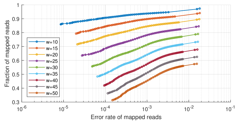
Figure 4.13: Effect of the window size parameter w on the error rate and sensitivity for simulated reads. Effect of window size on the proportion of mapped reads and the associated error rate (log scale) for 4 million simulated long reads (see Materials and Methods). A single curve contains points for each mapping quality threshold (MAPQ score), one point for each mapping quality threshold from 60 (leftmost) to 0 (rightmost).

In the context of multi-part index accuracy, simulated long reads were aligned using Minimap2 with single reference index (single-idx), partitioned index without merging (part-idx-no-merge) and partitioned index with merging (part-idx-merged). Partitioned indexes with 2, 4, 8 and 16 parts were tested. For each instance, we evaluated base-level alignments (default SAM output) as well as locus- or block-based alignment (default PAF output without CIGAR information). To evaluate alignment accuracy, Mapeval utility in Paftools was used with default options, which consider only the longest primary alignment for a read. However, Paftools assumes that all alignments for a particular read reside contiguously. Hence, for part-idx-no-merge, we first sorted the alignments based on the read ID. The output from Paftools contains the accumulative mapping error rate and the accumulative number of mapped reads for different mapping quality thresholds [176]. The fraction of mapped reads is taken as a measure of sensitivity.

4.4.4.2 Nanopore sequencing data

We could not find a suitable Nanopore simulator. Published Nanopore simulators explored at the time of writing had issues such as dependence on Minimap2 (would cause a bias), unavailability of trained models for human genome, being unstable or unavailability of source code. (For instance DeepSimulator [177] and NanoSim [178] are dependent on Minimap2, SNaReSim [179] code was not available.) Hence we used a a dataset from the publicly available NA12878 sample (rel3-nanopore-wgs-84868110-FAF01132 [56]). The dataset had 689,781 reads with about 5.5 Gbases. We aligned this dataset to the human genome using a 16-part index with merging (part-idx-merged) and without merging (part-idx-no-merge) with base-level alignment. Then we compared those outputs by generating some alignment summary metrics with the result from a single reference index (single-idx). We initially attempted to perform an extensive comparison using tools such as CompareSAMs utility in Picard [58] and qProfiler utility in AdamaJava [180]. They crashed probably because they are designed to be worked with short reads. Hence, we first obtained simple summary metrics using samtools[57] together with custom Linux shell scripts. Then we performed an extensive read by read comparison between the SAM outputs from single-idx and part-idx-merged using a custom tool written in C. The tool sequentially reads two SAM files while loading all the alignments for a particular read to the memory at a time. For a particular read, it compares and then outputs the alignment entries when the mappings positions between the two sets are disparate or if mapped only in one set (discordant). On these disparate and discordant mappings we used bedtools[181] to find overlaps with the UCSC repeatMasker track.

The same above NA12878 dataset was used to measure the runtime of partitioned indexes. The runtime and the peak memory usage were measured using the GNU time command line utility.

The ultra-long chromothriptic read was sourced from an unpublished patient-derived dataset generated in house (see Garsed et al[173] for more details on the cancer cell line). The data was generated on a MinION MkI sequencer (MN16218) with MinKNOW version 1.1.17 on a first generation R9 flowcell (MIN105, no spot-on loading, flow cell ID FAD24075) using the SQK-RAD001 library preparation kit from ONT. The raw data for the read was live base called with MinKNOW 1.1.17 and produced an average fastq score of 7.8.

4.5 Summary

Aligning long reads generated from third generation high-throughput sequencers to large reference genomes is possible on computers with limited volatile memory. Parameter optimisation alone cannot substantially reduce memory usage without considerably sacrificing alignment quality. Partitioning an alignment index, saving the internal state, and merging the output a posteriori substantially reduces memory usage. This strategy reduces the memory requirements for aligning Nanopore reads to the human reference genome from 11GB to less than 2GB, with minimal impact on accuracy.

4.6 Data Availability

The datasets generated and analysed during the evaluation are available in the figshare repository [182] [https://doi.org/10.6084/m9.figshare.6964805.v1].

Chapter 5 GPU Accelerated Adaptive Banded Event Alignment for Rapid Comparative Nanopore Signal Analysis

  This chapter is available as a pre-print in bioRxiv under the CC-BY-NC 4.0 International license at [26]. An adapted version of this chapter is published in BMC Bioinformatics: H. Gamaarachchi, C. W. Lam, G. Jayatilaka, H. Samarakoon, J. T. Simpson, M. A. Smith, and S. Parameswaran, “GPU Accelerated Adaptive Banded Event Alignment for Rapid Comparative Nanopore Signal Analysis,” BMC Bioinformatics 21, 343 (2020). DOI: https://doi.org/10.1186/s12859-020-03697-x.
 

Nanopore sequencing has the potential to revolutionise genomics by realising portable, real-time sequencing applications, including point-of-care diagnostics and in-the-field genotyping. Achieving these applications requires efficient bioinformatic algorithms for the analysis of raw nanopore signal data. For instance, comparing raw nanopore signals to a biological reference sequence is a computationally complex task despite leveraging a dynamic programming algorithm for Adaptive Banded Event Alignment (ABEA)—a commonly used approach to polish sequencing data and identify non-standard nucleotides, such as measuring DNA methylation. Here, we parallelise and optimise an implementation of the ABEA algorithm (termed f5c) to efficiently run on heterogeneous CPU-GPU architectures. By optimising memory, compute and load balancing between CPU and GPU, we demonstrate how f5c can perform ~3-5$\times$ faster than the original implementation of ABEA in the Nanopolish software package. We also show that f5c enables DNA methylation detection on-the-fly using an embedded System on Chip (SoC) equipped with GPUs. Our work not only demonstrates that complex genomics analyses can be performed on lightweight computing systems, but also benefits High-Performance Computing (HPC). The associated source code for f5c along with GPU optimised ABEA is available at https://github.com/hasindu2008/f5c.

5.1 Introduction

Advances in genomic technologies have given rise to a new era in biomedical sciences, improving the feasibility and accessibility of rapid species identification, accurate clinical diagnostics, and specialised therapeutics, amongst other applications. Whole genome sequencing involves ‘reading’ the entire DNA sequence of a cell, revealing the genetic variation that underlies biological diversity and the onset of disease. A human genome encompasses two copies of ∼3.2 billion DNA nucleotides, or ‘letters’. Therefore, analysing the data generated by contemporary high-throughput sequencing technologies typically requires high-performance computing support.

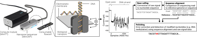
Figure 5.1: Nanopore portable sequencer and associated data analysis

The latest generation (third generation) of sequencing technologies can generate ultra-long DNA ‘reads’ from single molecules in real-time. In particular, Oxford Nanopore Technologies (ONT) manufacture a pocket-sized sequencer called MinION (Fig. 5.1), a relatively inexpensive and portable sequencing device capable of sequencing in-the-field (e.g. remote area with no network connectivity) or at the point-of-care (e.g. hospital, clinic, pharmacy).

In contrast to ‘second’ generation sequencers, which produce highly accurate short reads through enzymatic synthesis of the complementary strand of DNA, nanopore sequencing measures characteristic disruptions in the electric current (referred to hereafter as raw signal) when DNA passes through a biological nanopore (Fig. 5.1). A consumable flowcell containing an array of hundreds or thousands of such nanopores is loaded into the sequencing device (e.g. MinION), which is coupled to a generic (e.g. laptop) or dedicated (e.g. MinIT) compute module to acquire sequence data and base-call (the process of converting the raw signal to nucleotide characters) in parallel.

Nanopore sequencing offers several benefits over other technologies, including ultra-long reads (>1 Mbases), detection of non-standard DNA bases or biochemically modified DNA bases, and real-time analysis, at the expense of a higher error-rate, which is predominantly caused by the conversion of the raw signal into DNA bases via probabilistic models (referred to as ‘base-calling’). To overcome base-calling errors, the raw signal can be revisited a posteriori (see the polishing step in Fig. 5.1). Such a posteriori ‘polishing’ can correct for base-calling errors by aligning raw signal to a biological reference sequence, thus identifying idiosyncrasies in the raw signal by comparing observed signal levels to expected levels at all aligned positions. This process can also reveal base substitutions (i.e. mutations) or base modifications such as 5-methylcytosine (5mC), a dynamic biochemical modification of DNA that is associated with genetic activity and regulation. Detecting 5mC bases is important for the study of DNA methylation in the field of epigenetics.

A crucial algorithmic component of polishing is the alignment of raw signal–a time series of electric current to a biological reference sequence. One of the first raw nanopore signal alignment is implemented in the popular tool Nanopolish [104], which employs a dynamic programming strategy referred to as Adaptive Banded Event Alignment (ABEA). ABEA is one of the most time consuming steps when analysing raw nanopore data. For instance, when performing methylation detection with Nanopolish, the ABEA step consumes ~70% of the total CPU time. Consequently, it is important to investigate strategies to reduce the runtime of ABEA to improve the turnaround time of certain nanopore sequencing applications, such as real-time polishing or methylation detection.

In this study, we dissect the ABEA algorithm to optimise and parallelise its use on diverse hardware platforms, including Graphics Processing Units (GPUs). Adapting this ABEA algorithm for the GPU is not a straight forward task due to three main factors: (i) Read lengths vary significantly (from ~100 to >1M bases), thus requiring millions to billions of dynamic memory allocations—an expensive operation in GPUs. (ii) Inefficient memory access patterns which are not ideal for the GPUs having relatively less powerful and smaller caches (compared to CPUs) result in frequent instruction stalls. (iii) Varying read lengths cause irregular utilisation of the GPU cores.

We overcome the above mentioned challenges by: (i) employing a custom heuristic-based memory allocation scheme; (ii) tailoring the algorithm and the GPU user-managed cache to exploit cache-friendly memory access patterns; and, (iii) using a heuristic based work-partitioning and load-balancing scheme between the CPU and GPU.

We demonstrate the utility of our GPU optimised ABEA by incorporating to a completely re-engineered version of the popular methylation detection tool Nanopolish. First, we re-engineered the original Nanopolish methylation detection tool to efficiently utilise existing CPU resources, which we refer to as f5c. Then, we incorporated our GPU optimised ABEA algorithm into the re-engineered f5c. We demonstrate how f5c enables DNA methylation detection using nanopore sequencers in real-time (i.e. on-the-fly processing of the output) by using an embedded System on Chip (SoC) equipped with a GPU. We also demonstrate how f5c benefits a wide range of computing systems from embedded systems and laptops to workstations and high performance servers.

The key contributions of this paper are: (i) the first example of GPU acceleration and optimisation of raw signal alignment algorithm; (ii) f5c, a re-engineered and optimised version of the popular DNA methylation detection tool Nanopolish; and, (iii) real-time detection of DNA methylation using a lightweight and portable embedded system (previously only possible on high-performance servers).

In the rest of the paper, we discuss the background of nanopore sequencing and ABEA algorithm in Section 5.2, related work in Section 5.3, methodology in Section 5.4, results in Section 5.5, followed by the discussion and future work in Section 5.6. The associated tool that includes the GPU-based acceleration is available at https://github.com/hasindu2008/f5c.

5.2 Background

Basic terms and concepts of DNA sequencing and data analysis are given in Section 5.2.1. Section 5.2.2 briefly explains methylation calling, an example nanopore data analysis workflow. Section 5.2.3 explains the Adaptive Banded Event Alignment (ABEA) algorithm, the algorithm which is optimised in this paper for execution on a CPU-GPU heterogeneous architecture. In Section 5.2.4, a brief account of GPU architectures and the programming methods for GPUs.

5.2.1 Nanopore sequencing and analysis

5.2.1.1 Whole genome sequencing

The genome is a long sequence composed of four types of nucleotide bases: adenine (A), cytosine (C), guanine (G) and thymine (T). Nucleotide bases will be simply referred to as bases hereafter. The human genome is around 3.2 gigabases (Gbases) long and is composed of 23 pairs of chromosomes (46 chromosomes in total), where each chromosome is a single molecule of continuous deoxyribonucleic acid (DNA) polymer. The process of reading strings of contiguous bases is called sequencing, and the resulting strings of bases are called reads. In order to be sequenced, DNA molecules must be extracted and purified from cells before being biochemically prepared for sequencing. This library preparation process can fragment chromosomes (especially large ones) into smaller segments–either intentionally or incidentally–which are ‘read’ by the sequencer. Given that samples contain multiple cells, and thus several distinct DNA molecules, and that sequencing may introduce errors, it is desirable to generate enough reads to cover a particular position several times. The average number of reads at a given position is termed sequencing coverage. High coverage facilitates the characterisation of genetic variation and correct for errors. A human genome sequenced at around 20$\times$ average coverage corresponds to around 64 Gbases of sequencing reads.

5.2.1.2 DNA methylation

DNA undergoes naturally regulated biochemical modification through the addition of a methyl group to certain bases. Methylation is reversible and can control the activity of a DNA segment, such as turning the expression of genes on or off, without modifying the genetic code itself—a process called epigenetic regulation. DNA methylation is dynamically regulated during normal biological development and in function of environmental factors; it plays an important role in disease aetiology and clinical diagnostics [183, 184, 185]. Methylation of cytosine (‘C’) bases is of particular interest in human biology, where CpG dinucleotides ( ‘C’ base followed by a ‘G’ base) are dynamically methylated in normal development and disease [186, 187, 188].

5.2.1.3 Nanopore sequencing and the raw signal

Nanopore sequencing is a third generation sequencing technology that involves physical observation of atomic properties of DNA fragments using a nanometer scale biological pore coupled to an ammeter (see Fig. 5.1). The pore acts as a bottleneck to generate characteristic disruptions in ionic current (in the range of pico-amperes) that are indicative of the molecules passing through the pore. The size and nature of the pore influence the measured instantaneous current and how it is subsequently analysed. Oxford Nanopore Technologies (ONT) sequencing devices measure DNA strand passing through biological nanopores composed of recombinant (or ‘designer’) proteins at an average speed of ~450 bases/s while the current is sampled and digitised at ~4000 Hz. The instantaneous current measured in ONT nanopore depends on 5-6 contiguous bases [189]. The measured signal also presents stochastic noise due to several factors, such as homopolymers (same base repeating multiple times) which produce constant current levels, contaminants in the sample, entanglement of long DNA strands, depletion of ions, etc [190]. Additionally, the movement speed of the DNA strand through the pore can vary, causing the signal to warp in the time domain [190]. The raw signal is converted into character representations of DNA bases (e.g. A,C,G,T) using artificial neural networks, generating a typical accuracy >90% for single reads [55]. This conversion process is referred to as base-calling and the software tools that perform this conversion are referred to as base-callers. Please refer to [189] for a detailed discussion of ONT sequencing.

An example of a raw nanopore signal is shown in Fig. 5.2(a) using blue coloured line. Assume that the signal is generated from the DNA sequence GAATACGAAAATCATTA which passed through the nanopore. In this example, the instantaneous current of the signal is affected by a string of 6 contiguous bases, known as a 6-mer (or a k-mer in general). Let us assume that the annotation of the signal to the corresponding k-mers is known (the process of getting this annotation is detailed in Section 5.2.2). The 6-mers in the sequence and the corresponding segments in the raw signal are marked using vertical grey lines in Fig. 5.2(a). When the DNA sequence GAATACGAAAATCATTA moves through the pore, the first 6-mer is GAATAC. Similarly, the subsequent 6-mers are AATACG, ATACGA, TACGAA, …, TCATTA. True annotation (depicted by dotted green coloured step function in Fig. 5.2(a)) corresponds to the ideal average level of current for each k-mer. These ideal average values are obtained using the pore-model provided by ONT, which is elaborated in Section 5.2.2. The red coloured step function corresponds to an event—detailed in Section 5.2.2.

To deduce the sequence from the k-mers, the base at the centre (3rd base) of each k-mer is taken, as shown on the bottom of Fig. 5.2(a). For instance, we take A from GAATAC, T from AATACG, C from TACGAA and etc. Hence, we obtain a sequence ATACGAAAATCA which is a part of the original sequence GAATACGAAAATCATTA. Note that the beginning and the end of the sequence (GA at the beginning and TTA at the end) are clipped.

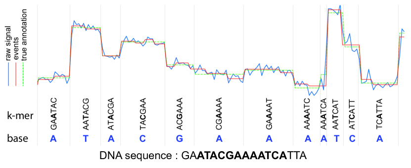
(a) An example nanopore raw signal and events

(b) an example pore-model

Figure 5.2: Illustration of a nanopore raw signal, events and pore-model

5.2.1.4 Nanopore read length distribution

The length of the reads generated from nanopore sequencers can vary from several hundred bases to even more than 2 million bases. A typical sequencing run of a particular sample (which completes after 48-64 hours) generates millions of such reads. The distribution of the read lengths varies in function of DNA integrity, extraction protocols, and sample preparation methods. Example distributions for three different samples are shown in Fig. 5.3, where both x and y axes are in logarithmic scale. The average read length of a sample typically falls between 8-20 Kilobases.

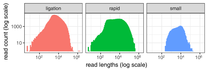
Figure 5.3: example nanopore read length distributions

5.2.1.5 Sequence alignment/mapping in the base-space

Once a nanopore read is base-called, the sequence is aligned to a reference sequence (see Fig. 5.1). A reference sequence consists of a previously generated consensus sequence (such as the human genome reference). Sequence alignment involves global optimisation algorithms to identify the most similar target and to compare any differences between sequences. Compared to biologically occurring variation in individual genomes (<1% difference to the reference), the error-rate of nanopore sequencing is relatively high (5-10%). Thus, sequence alignments derived from nanopore reads are distinct in nature from previous sequencing technologies (such as highly accurate short reads). Consequently, unique analytic tools must be considered when aligning such reads. Alignment tools such as Minimap2 [101] that employ a hash table based genome index followed by a base-level dynamic programming alignment step can successfully align long and noisy reads.

5.2.1.6 Polishing/Downstream processing using raw signal

The base-space alignment discussed previously in Section 5.2.1.5 is followed by ‘polishing’, a downstream processing step which utilises both the base-space alignment results and the raw signal (see Fig. 5.1). The polishing step reuses the raw signal to recover the lost biological information during base-calling. This polishing step can be to correct errors during base-calling or to detect modified nucleotide bases (eg: DNA methylation).

Previous research has shown that identification of genetic variants can be improved up to an accuracy of more than 99% by using raw signal data from multiple overlapping reads [56, 103]. Thus, the downstream analysis that reuses raw signal data could correct for base-calling errors. It has also been shown that methylated C bases can be differentiated from non-methylated C bases by the use of signal data, using algorithms such as the one implemented in the software package Nanopolish [104]. Thus, the downstream analysis that reuses raw signal data could detect modified nucleotide bases.

Signal-space alignment is one of the crucial steps performed in these downstream analyses such as error correction and modified base detection. This signal alignment step is described in the context of modified base detection in the following sections.

5.2.2 Methylation calling

As discussed above, important biological information is lost during base-calling. Some base-calling models may not accommodate methylated data, either because they are trained on unmethylated sequences, or because they abstract away non-canonical bases. Therefore, these molecules may be erroneously classified as unmethylated bases. The process of identifying methylation is known as methylation calling.

As implemented in Nanopolish, methylation calling requires: 1, raw signals; 2, base-called reads; and 3, base-space alignment to a reference genome (output of the sequence alignment step described above). For a given read, the main steps for methylation calling are: 1, event detection; 2, signal-space alignment; and 3, Hidden Markov Model (HMM) profiling. These steps are performed for each individual read in the data set.

Event detection is the time series segmentation of the raw signal based on sudden signal level changes. Each segment is called an event and is typically denoted using the mean ($\mu_{\bar{x}}$), standard deviation ($\sigma_{\bar{x}}$) and the duration of the raw signal samples ($n_{\bar{x}}$) pertaining to the particular segment. The red step function in Fig. 5.2(a) denotes such detected events by plotting the mean value of the samples ($\mu_{\bar{x}}$) corresponding to the segment. Note that in Fig. 5.2(a), events (red line) roughly match to the true annotation (dotted green line), nevertheless, are not exactly the same. Mostly, the signal has been over-segmented (eg: portion corresponding to k-mer CGAAAA has been segmented into 3 events) and seldom under-segmented (eg: k-mer AAATCA).

To obtain the true annotation in Fig. 5.2(a), the events detected in the event detection step are aligned to a generic k-mer model signal. This generic k-mer model signal is derived from the base-called sequence and a pore-model provided by ONT. The pore-model corresponds to a table of all possible k-mers matched to their mean signal value and standard deviation (4⁶ k-mers if k is 6, as shown in Fig. 5.2(b)). For each 6-mer in the base-called read, the corresponding entry in the pore model (mean,sd) is obtained and these mean,sd pairs form the generic k-mer model signal. Nanopolish aligns the events from the event detection step to this generic k-mer model signal by using the algorithm named Adaptive Banded Event Alignment (ABEA) explained in Section 5.2.3.

ABEA above produces the alignment between the events and the k-mers in the base-called read. The base-space sequence alignment then is used to deduce which event corresponds to a given k-mer in the reference genome. Finally, this alignment between the events and the k-mers in the reference genome are subjected to Hidden Markov Model (HMM) profiling to identify if a given base is methylated or not.

5.2.3 Adaptive Banded Event Alignment (ABEA)

Modified versions of the SK (explained in section 2.2.2) algorithm are used for event-space alignment as exemplified in Nanopolish and is referred to as Adaptive Banded Event Alignment (ABEA). In ABEA, the events are aligned to the k-mers of the base-called read (as stated in Section 5.2.2). As typically there are many more events than k-mers (usually by a factor 1.5-2) due to the frequent over-segmentation of events (discussed in Section 5.2.2), event alignment is even more difficult than base-space long read alignment if performed with static banding around the diagonal. Thus, an adaptive band is essential for event alignment.

The scoring function for signal alignment uses a 32 bit floating point data type, as opposed to 8-bit integer data type in sequence alignment. Furthermore, the signal alignment scoring function that computes the log-likelihood (which we elaborate shortly) is computationally expensive.

A simplified example of ABEA is shown in Fig. 5.4(a). In Fig. 5.4(a) the horizontal axis represents the events (results of the event detection step) and the vertical axis represents the ref k-mers (k-mers of the base-called read). The dynamic programming table (DP table) in Fig. 5.4(a) is for 13 events, indexed from e₀-e₁₂ vertically, and the ref k-mers, indexed from k₀-k₅ horizontally. As mentioned previously for computational and memory efficiency, only the diagonal bands (marked using blue rectangles) with a band-width of $W$ (typically $W$=100 for nanopore signals) are computed. The bands are computed along the diagonal from top-left (b0) to bottom-right (b17). Each cell score is computed in function of five factors: scores from the three neighbouring cells (up, left and diagonal); the corresponding ref k-mer; and, the event (shown for the cell e₆, k₃ via red arrows in Fig. 5.4(b), details of the computation is explained later). Observe that all the cells in the $n$^th band can be computed in parallel as long as the $n-1$^th and $n-2$^th bands are computed beforehand. To contain the optimal alignment, the band adapts by moving down or to the right as shown using blue arrows in Fig. 5.4(a). The adaptive band movement is determined by the Suzuki-Kasahara heuristic rule [102].

Algorithm 8 summarises the ABEA algorithm used in Nanopolish [104] and is explained with the aid of the example in Fig. 5.4(a).

Algorithm 8 Adaptive Banded Event Alignment

Input:

ref[] : the base-called read (1D char array)

model : pore-model (Fig. 5.2(b))

events[] : event table containing {$\mu_{\bar{x}}$,$\sigma_{\bar{x}}$,$n_{\bar{x}}$} of each event—1D {float,float,float} array

Output:

alignment[] : alignment denoted by a list of {event index,k-mer index}—1D {int,int} array

Intermediate:
      score[][] : scores of the cells in banded area—2D float array

trace[][] : back-track flags of the cells in banded area—2D char array

ll_idx[] : {event index,k-mer index} for each band’s lower left cell—1D {int,int} array

1:function align(ref,model,events)

2:     initialise_first_two_bands(score,trace,ll_idx) $\triangleright$ band b0 and b1 in Fig. 5.4(a), see line 20

3:     for i $\leftarrow$ 2 to n_bands do $\triangleright$ Iterate from b2 to b17 in Fig. 5.4(a)

4:         dir $\leftarrow$ suzuki_kasahara_rule(score[i-1]) $\triangleright$ score[i-1] is of the previous band

5:         if $dir==right$ then

6:              ll_idx[i] $\leftarrow$ move_band_to_right(ll_idx[i - 1]) $\triangleright$ see line 28

7:         else

8:               ll_idx[i] $\leftarrow$ move_band_down(ll_idx[i - 1]) $\triangleright$ see line 33

9:         end if

10:         min_j,max_j $\leftarrow$ get_limits_in_band(ll_idx[i]) $\triangleright$ get index bounds in current band^*

11:         for j $\leftarrow$ min_j to max_j  do $\triangleright$ Iterates through each cell in band i

12:              s,d $\leftarrow$ compute(score[i-1],score[i-2],ref,events,model) $\triangleright$ see Algorithm 9

13:              score[i,j] $\leftarrow$ s

14:              trace[i,j] $\leftarrow$ d

15:         end for

16:     end for

17:     alignment $\leftarrow$ backtrack(score, trace. ll) $\triangleright$ the trace-back red arrows in Fig. 5.4(c).

18:end function

19:

20:function initialise_first_two_bands(score,trace,ll_idx)

21:     score[0,*], trace[0,*] $\leftarrow-\infty,0$ $\triangleright$ Initialise first band b0

22:     score[1,*], trace[1,*] $\leftarrow-\infty,0$ $\triangleright$ Initialise second band b1

23:     ll_idx[0] $\leftarrow$ {$ei_{0}$,$ki_{0}$} $\triangleright$ $ei_{0}=1$ and $ki_{0}=-1$ in Fig. 5.4(a)^**

24:     ll_idx[1] $\leftarrow$ {$ei_{1}$,$ki_{1}$} $\triangleright$ $ei_{1}=1$ and $ki_{1}=0$ in Fig. 5.4(a)^**

25:     score[0,$si_{0}]$ $\leftarrow$ 0 $\triangleright$ $si_{0}$ is 0 is Fig. 5.4(a)^***

26:end function

27:

28:function move_band_to_right(ll_previous)

29:     ll_current.event_idx $\leftarrow$ ll_previous.event_idx + 1

30:     ll_current.kmer_idx $\leftarrow$ ll_previous.kmer_idx

31:end function

32:

33:function move_band_down(ll_previous)

34:     ll_current.event_idx $\leftarrow$ ll_previous.event_idx

35:     ll_current.kmer_idx $\leftarrow$ ll_previous.kmer_idx+1

36:end function

^*For instance, in Fig. 5.4(a) min_j=1,max_j=1 for b0 and b17; min_j=0,max_j=1 for b1; min_j=1,max_j=2 for b16; and, min_j=0,max_j=2 for the rest
^**these initial event and k-mer indices corresponding to the lower left of the band are computed with respect to band-width $W$
^***the score of cell that corresponds to k-mer index -1 in band b0 is initiliased to 0

The input to the Algorithm 8 are: 1, ref (the sequenced read in base-space—eg: GAATACG…); 2, events (the output of the event detection step mentioned in Section 5.2.2); and 3, model (pore-model—Fig. 5.2(b)). As mentioned in Section 5.2.2, the ABEA algorithm (Algorithm 8) attempts to align the events to the generic signal model (produced with the use of ref and the model) and outputs the alignment as event-ref pairs. The algorithm requires three intermediate arrays, namely score (2D floating point array), trace (2D byte array) and ll (1D pointer array) to formulate the intermediate state during alignment computation, which is the DP table shown in Fig. 5.4(a)). Note that, ll stands for lower-left, which holds the coordinate of the start point of the band.

The initialisation of the first two bands (b0 and b1) in Fig. 5.4(a) is performed by line 20 of Algorithm 8. Then, the outer loop (starting from line 3) iterates through rest of the bands from top-left to bottom-right of the DP table. The inner loop (lines 11-15) iterates through each cell in the current band bi. To ensure that only cells within the DP table are computed, the loop counter $j$ iterates from min_j to max_j, instead of 0 to $W-1$. Lines 4-9 of Algorithm 8 correspond to the movement of the band (corresponds to the blue arrows in Fig. 5.4(a)). Band movement is actuated by proper placement of the band in the static 2D arrays, score and trace via the array ll using the functions move_band_right and move_band_down.

Line 12 of the algorithm performs the cell score computation (explained in detail later) and generates a score and a direction flag for subsequent backtracking, which are henceforth stored in the arrays score and trace. When all the cells in the DP table are computed, the final operation is to find the actual alignment (event-ref pairs) through the backtracking operation (line 17 of Algorithm 8 and red trace-back arrows in Fig. 5.4(c)), which uses both the cell scores and the direction flags stored in trace.

The compute function (called at line 12 of Algorithm 5.4(a)) is elaborated in Algorithm 9. A number of heuristically determined constants suitable for Nanopore data, which are used during subsequent calculations are listed at the beginning of this algorithm. The first step of this algorithm is the computation of lp_emission, a log probability value (likelihood of the particular signal event being the particular ref k-mer), performed using the function elaborated in Algorithm 10. This computed lp_emission is used in lines 4-5 of Algorithm 9 along with the heuristically determined constants (lp_skip,lp_stay,lp_step) to compute three scores from the diagonal, left and up (score_d, score_u, score_l). The maximum of the three scores and direction from which the max score came (flags pertaining to diagonal, up or left) are returned as outputs from this function. The line 3 of Algorithm 9 refers to accessing the scores of the upward, left and diagonal cells which was previously mentioned with respect to cell e₆,k₃ and the red arrows in Fig. 5.4(b).

The log probability computation in Algorithm 10 involves floating point log probability computations. For the k-mer at the specific ref position, the pore-model table (Fig. 5.2(b)) is accessed to obtain the corresponding model values. This model_kmer (mean and the standard deviation of the particular model k-mer) and the mean value of the event is used for the log probability computation as shown in the Algorithm 10. Note that for event alignment neither the standard deviation or the duration of the event are used.

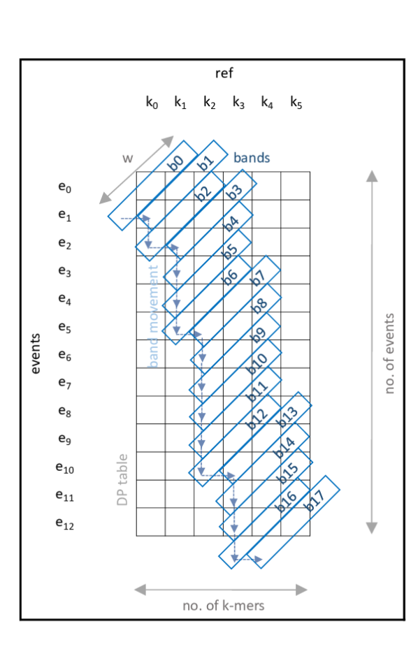
(a) band movement

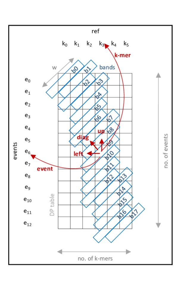
(b) computing a single cell score

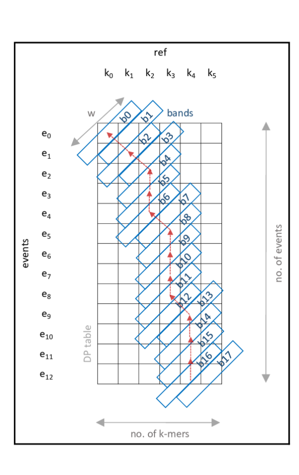
(c) trace-back

Figure 5.4: Adaptive Banded Event Alignment

Algorithm 9 Adaptive Banded Event Alignment - cell score computation

Constants:

$events\_per\_kmer=\frac{n\_events}{n\_kmers}$

$\epsilon=1^{-10}$

lp_skip $=\ln(\epsilon)$

lp_stay $=\ln(1-\frac{1}{events\_per\_kmer+1})$

lp_step $=\ln(1.0-e^{lp\_skip}-e^{lp\_stay})$

1:function computation(score_prev,score_2ndprev,ref,events,model)

2:     lp_emission $\leftarrow$ log_probability_match(ref,events,model) $\triangleright$ see Algorithm 10

3:     up,diag,left $\leftarrow$ get_scores(score_prev,score_2ndprev) $\triangleright$ see red arrows in Fig. 5.4(b)

4:     score_d $\leftarrow$ diag $+$ lp_step $+$ lp_emission

5:     score_u $\leftarrow$ up $+$ lp_stay $+$ lp_emission

6:     score_l $\leftarrow$ left $+$ lp_skip

7:     s $\leftarrow$ max(score_d,score_u,score_l)

8:     d $\leftarrow$ direction from which the max score came

9:end function

Algorithm 10 Adaptive Banded Event Alignment - log probability computation

1:function log_probability_match(ref,events,model)

2:     event,kmer $\leftarrow$ get_event_and_kmer(ref,events) $\triangleright$ see red arrows in Fig. 5.4(b)

3:     $x\leftarrow$ event.mean

4:     model_kmer $\leftarrow$ get_entry_from_poremodel(kmer,model)

5:     $\mu\leftarrow model\_kmer.mean$

6:     $\sigma\leftarrow model\_kmer.stdv$

7:     $z\leftarrow\frac{x-\mu}{\sigma}$

8:     lp_emission $\leftarrow\ln(\frac{1}{\sqrt{2\pi}})-\ln(\sigma)-0.5z^{2}$

9:end function

The above elaboration covers the ABEA algorithm to a sufficient enough level to explain our GPU implementation and optimisations. Therefore, implementation details of checking out of bound array accesses and the backtracking process were not discussed. Furthermore, the concept of the ‘trim state’ and ‘event scaling’ were not discussed as the control flow of the algorithm are not affected by them. Thus, those details not vital for the elaboration GPU implementation. However, for the sake of completeness, a brief account of this ‘trim state’ and ‘read-model scaling’ are given below.

The raw signal may contain samples at the beginning/end that may be ignored by the base-caller and hence does not contribute to the base-called sequence. These samples may be open pore signal immediately before or after the DNA molecule is detected (i.e. the electric current when nothing is in the nanopore), or perhaps part of the adaptor (molecules bounds to the ends of the DNA molecules to enable sequencing). The ‘trim states’ allow the alignment to ignore these samples, since such samples should not be considered to be part of the base-called read.

Due to reasons such as slight variations between different nanopores and characteristic changes of the same nanopore with time, an event will not directly match the pore-model in Fig. 5.2(b) [191]. Therefore, to account for these variations either the events or the pore-model should be scaled on a per-read basis. In Nanopolish, two scaling parameters namely shift and scale are estimated on a per-read basis, prior to ABEA algorithm, using a ‘Method of Moments’ approach [191]. Then, during ABEA, the pore-model mean values are scaled using these two parameters. The scaling should be performed at line 5 of Algorithm 10 as $\mu\leftarrow model\_kmer.mean\times scale+shift$ instead of directly assigning $model\_kmer.mean$ to $\mu$.

5.2.4 GPU architecture and programming

Graphics Processing Units (GPUs) were originally designed as co-processors for graphics processing and rendering. Graphics processing and rendering algorithms involve pixel-wise operations which expose fine-grained parallelism, thus GPUs consists of hundreds of compute cores to perform parallel processing. Eventually, the concept of general purpose graphics processing units (GPGPU) emerged where the GPUs were exploited to accelerate compute intensive, yet highly parallelism portions of general purpose algorithms. GPUs are quite popular in scientific computations due to the significant speedup when used for common matrix manipulation which contains fine-grained parallelism. From around a decade ago, GPUs which are explicitly designed for high performance computers are available (e.g., Tesla GPUs from NVIDIA).

GPUs are of Single Instruction Multiple Data (SIMD) architecture (or more accurately Single Instruction Multiple thread, as stated by NVIDIA), where multiple threads run the same stream of instructions in parallel yet on different data. Conversely, CPUs are of Multiple Instruction Multiple Data (MIMD) architecture, where each thread runs its own instruction sequence and own data stream, independent of the others. GPUs have hundreds or even thousands of processing cores while a CPU would maximally have a few dozen cores. However, the GPU cores are relatively less complex (fewer instructions, smaller caches, no sophisticated branch prediction units etc.) and run at a lower clock speed when compared to a CPU. Due to these significant differences between CPU and GPU architectures, serial algorithms designed and developed for the CPUs are not suitable for execution on GPUs. Such algorithms have to be adapted and parallelised in a way that the GPU architectural features are efficiently used.

NVIDIA provides a programming model/framework for programming their GPUs for general purpose computations, called Compute Unified Device Architecture (CUDA). CUDA includes CUDA C/C++ (extended C/C++ syntax) and an Application Programming Interface (API) to provide a platform to write programs for the NVIDIA GPU. We used this CUDA C/C++ for our GPU implementation of the Adaptive Banded Event Alignment algorithm.

We will now briefly give GPU/CUDA related terms. Readers are advised to refer to [192] and [193] for further information.

A GPU kernel is a function that is executed on a GPU. A GPU kernel is written from the execution perspective of a single GPU thread. These GPU kernels will run in parallel, based on the parameters specified with the function call, known as the thread configuration. This thread configuration in CUDA is an abstraction which employs a hierarchy of threads. In the thread hierarchy, a group of threads are known as a block. A group of blocks form a grid. Instances of a single kernel are executed in a single grid. Blocks and grids can be 1 dimensional, 2 dimensional or 3 dimensional. The presence of this thread hierarchy lets the programmer organise and map the threads conveniently to a grid. These logical threads would be mapped to the hardware cores automatically by the underlying driver software and hardware.

A thread block consists of one or more thread warps. A warp is a group of threads sharing the same program counter. A data dependent conditional branch inside a warp causes the threads to execute each code path while disabling threads that are not in the path, known as warp divergence. The warp divergence affects the performance and should be minimised.

The occupancy is the percentage of the number of active warps to the maximally supported warps on the GPU. A lesser occupancy leads to under utilisation of GPU resources. Thus, a higher occupancy is preferable for better utilisation of GPU resources.

GPUs also employ a memory hierarchy. Relatively larger but slow Dynamic Random Access Memory (DRAM) that forms the lowest level in the memory hierarchy is known as global memory. Global memory is typically allocated using cudaMalloc() API function. Memory allocated in this global memory can be exclusively accessed by all the threads in the grid. The next level in the memory hierarchy which is made of relatively fast, yet smaller SRAM is called shared memory. Shared memory is allocated on a per-thread-block basis and is shared by all the threads in the block. Shared memory can be called user managed cache (more accurately a programmer managed cache) as the programmer is expected to identify and load frequently accessed data to the shared memory. In addition, there are one or more levels of SRAM caches managed by the hardware. The registers are the fastest and highest in the hierarchy and are allocated by the compiler on a per-thread basis.

The global memory can be easily saturated when hundreds of threads compete to access the memory at the same time. Thus, memory accesses should be batched such that contiguous threads access contiguous memory locations. This process is referred to as memory coalescing and reduces global memory requests thus reducing the impact on performance compared to scattered memory accesses. Additionally, the programmer could utilise the shared memory to load and store frequently accessed data, which also reduces global memory traffic.

5.3 Related work

An algorithm to call methylation using the raw signal from ONT sequencers was introduced by Simpson et al. [104]. The associated C++ based implementation of this algorithm is a sub-module under the open source tool Nanopolish. Nanopolish was designed to run on high-performance computers and is not lightweight or suitable for deployment on embedded systems.

The signal-space alignment algorithm, termed Adaptive Banded Event Alignment (ABEA), used in Nanopolish is a customised version of the Suzuki-Kasahara alignment algorithm [102] for base-level sequence alignment. According to the best of our knowledge, neither of these algorithms (ABEA or Suzuki-Kasahara) have GPU accelerated versions. The root origins of these algorithms are dynamic programming sequence alignment algorithms, such as Smith-Waterman and Needleman-Wunsch. A number of GPU accelerated versions for Smith-Waterman exist in previous research [134, 194, 195] [194] [195]. However, the Smith-Waterman algorithm has a compute complexity of $O(n^{2})$ and is most practical when the sequences are short, especially when millions of sequences need to be aligned. As nanopore sequencers can produce reads >1 million bases long, computing the full DP table for such reads using SW would require >10¹² computations and hundreds of gigabytes of RAM—and even more if aligning raw nanopore signals.

Heuristic approaches such as banded Smith-Waterman attempt to reduce the search space by limiting computation along the diagonal of the DP table. While the approach is suitable for Illumina short reads, it is less so for noisy long nanopore reads as substantial band-width is required to contain the alignment within the band. The Suzuki-Kasahara algorithm uses a heuristic that allows the band to adapt and move during the alignment, thus containing the optimal alignment within the band but allowing large gaps in the alignment. Modified versions of the adaptive banded alignment algorithm are used for signal-space alignment, as exemplified in Nanopolish. The band-width (width of the band) used for signal-space alignment is typically higher (~100) compared to other banded algorithms used for sequence alignment. In addition, the scoring function for signal alignment uses a 32 bit floating point data type, as opposed to 8-bit integers in sequence alignment. Furthermore, the signal alignment scoring function that computes the log-likelihood is computationally expensive. Taken together, these reasons motivated us to consider using GPUs to speedup the computation of signal-space alignment.

The portable compute module, MinIT, manufactured by ONT is composed of a NVIDIA SoC [196] that exploits GPUs for performing live base-calling, which can perform base-calling at a speed of ~150 Kbases per second, thus keeping up with the MinION sequencer’s output. In addition, our previous work has optimised the popular Minimap2 [101] sequence alignment tool (which typically requires ~16GB memory) for reduced peak memory usage, enabling the software to be executed on embedded processors [25]. The data processing steps required for methylation calling are thus possible to run on embedded processors, therefore supporting the implementation of a portable, offline DNA methylation detection application that would facilitate such analyses in the field.

Load balancing between the CPU and GPU for heterogeneous processing has been explored for areas such as fluid dynamics [197] and conjugate gradient method [198]. However, nanopore data have different characteristics compared to aforementioned applications which are predominately based on matrices. Furthermore, the signal-space alignment algorithm is different from linear algebra algorithms used in these fields. We exploit characteristics of Nanopore data and algorithms to perform memory, compute and load balancing optimisations.

5.4 Methodology

To optimise the performance on GPUs, we process a batch of reads (original source code processes a read at a time) at a time. Such batch processing minimises data transfer initialisation overhead (between RAM and GPU memory); reduces the GPU kernel invocation overhead; and, allows parallelism which sufficiently occupies all available GPU cores. The execution flow follows the typical GPU programming paradigm, which is elaborated in Algorithm 11. In Algorithm 11, gpu_alignment(…) refers to the GPU implementation of the Adaptive Banded Event Alignment (CPU algorithm is elaborated in Algorithm 8). We present our methodology in three steps: parallelisation and compute optimisations in Section 5.4.1; memory optimisation in Section 5.4.2; and, the resource optimisation through heterogeneous processing in Section 5.4.3.

Algorithm 11 Outline of execution flow

1:for batch of $n$ reads do

2:     … $\triangleright$ CPU processing steps before the Adaptive Banded Event Alignment eg: event detection

3:     $memcpy\_ram\_to\_gpu(...)$ $\triangleright$ copy inputs of the Adaptive Banded Event Alignment to the GPU memory

4:     $gpu\_alignment(...)$ $\triangleright$ Perform the event alignment on the GPU

5:     $memcpy\_gpu\_to\_ram(...)$ $\triangleright$ copy results back to the RAM

6:     … $\triangleright$ CPU processing steps after the alignment eg: HMM

7:end for

5.4.1 Parallelisation and compute optimisations

The GPU implementation of the Adaptive Banded Event Alignment (ABEA) algorithm is broken into three GPU kernels. Breaking down into the three GPU kernels allows for efficient thread assignment based on the workload type, synchronisation of all GPU threads (a GPU kernel execution is inherently a synchronisation barrier [192]) and minimising warp divergence compared to a big all-in-one GPU kernel.

The three GPU kernels are:

• pre-kernel - Initialising the first two bands of the dynamic programming table (corresponds to line 2 of algorithm 8) and pre-computing frequently accessed values by the next GPU kernel;

• core-kernel - The filling of dynamic programming table which is the compute intensive portion of the ABEA algorithm (corresponds to line 3-16 of Algorithm 8 composed of nested loop); and,

• post-kernel - Performs backtracking (corresponds to line 17 of algorithm 8)

5.4.1.1 pre-kernel

The pre-kernel initialises the first two bands of the dynamic programming table (initialisation performed at line 2 of Algorithm 8 on CPU). The pre-kernel also pre-computes the values in a data structure called kcache, a newly introduced data structure in the GPU implementation that improves cache hits during the subsequent execution of the core-kernel.

A simplified version of the pre-kernel is in Algorithm 12 and thread configuration for the invocation of the pre-kernel is in Fig. 5.5. Note that the GPU kernel is presented (as is always the case) from the perspective of a single GPU thread in Fig. 5.5.

Each cell in Fig. 5.5 represents a GPU thread denoted as t, where the subscripts x and y denotes the thread index along the x-axis and the y-axis respectively. The thread grid in Fig. 5.5 is composed of n thread blocks, where n is the number of reads in the batch. Each thread block contains WX threads where WX is the nearest upper ceiling multiple of 32 to the band-width W (band-width of the ABEA algorithm); i.e. $WX=(int)\frac{W+31}{32}\times 32$ For instance, if W=100, WX is 128. The reason for taking a multiple of 32 is due to performance attributed by a thread block size that a multiple of the warp size (warp size is 32 currently) [193] . As shown in Fig. 5.5, a single thread block composed of WX threads is assigned to a single read.

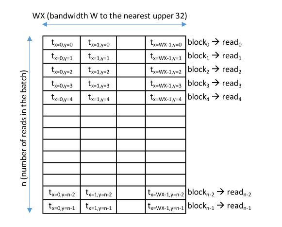
Figure 5.5: Thread configuration of pre-kernel

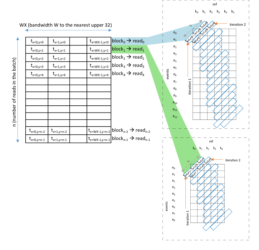
Figure 5.6: Thread assignment of pre-kernel. The assignment for the first two reads are shown. Each thread block has a read assigned to it (block₀ refers to threads $t_{X=0,y=0}$ to $t_{x=WX-1,y=0}$, and read₀ is processed by all threads in block₀; similarly, block₁ refers to $t_{X=0,y=1}$ to $t_{x=WX-1,y=1}$ and read₁ is processed by threads in block₁).

In the Algorithm 12, lines 2-3 get the thread index of the thread being executed, i.e. the thread indices denoted as x and y in Fig. 5.5. Line 4 obtains the memory pointers of the input array ref; intermediate arrays score and trace; and the kcache, the use in which is explained in the memory optimisation Section (Section 5.4.2).

Lines 5-8 of Algorithm 12 initialises the first two bands of the dynamic programming table (which was performed at line 2 of original CPU Algorithm 8). The kernel is in from the perspective of a single thread and thus a single cell is initialised by a single thread. The collective execution of all the threads in Fig. 5.5, effectively sets a band for all the reads in the batch in parallel, which is illustrated in Fig. 5.6. Note that, only the first two reads are elaborated in Fig. 5.6, and in reality each thread block has a read assigned to it. In Fig. 5.6, each cell in band₀ (marked as iteration 1) contains the index of the thread which performs the initialisation at line 6 of Algorithm 12. Similarly, iteration 2 corresponds to line 7 of Algorithm 12.

The if condition on line 5 of Algorithm 12 is to limit the threads to the width of the band $W$, a consequence of selecting $WX$ which is a multiple of 32 (as stated previously). Note that there is a 1024 thread limit for a block [192] in current NVIDIA CUDA/GPU architecture, thus our implementation will only work for a maximum band-width of 1024. This limit is more than sufficient for a typical $W$ of 100 in ABEA.

Line 10-11 of Algorithm 12 initialises the index of the lower left band which corresponds to line 23-24 of Algorithm 8. Note that this initialisation is executed by one thread per read (thread id 0 along y-axis). Lines 13-16 in Algorithm 12 initialises kcache. As stated previously kcache is a newly introduced array for the GPU implementation to minimise random accesses to the GPU memory during the core-kernel and will be explained in Section 5.4.1.2. Note that, this kcache initialisation in line 13-16 is also executed by one thread per read (thread id 0 along y-axis). The loop in 13-16 can be further parallelised; however, as the time spent on pre-kernel is comparatively negligible (see results), further parallelising this loop is superfluous.

Algorithm 12 Adaptive Banded Event Alignment - pre-kernel

1:function align_pre(…,model) $\triangleright$ … refers to other arguments which are later explained Section 5.4.2

2:     j $\leftarrow$ thread index along x $\triangleright$ the x subscript of a thread Fig. 5.5

3:     i $\leftarrow$ thread index along y $\triangleright$ the y subscript of a thread Fig. 5.5

4:     (ref,score,trace,ll_idx,kcache) $\leftarrow$ get_cuda_pointers(i,…) $\triangleright$ get memory pointers of the arrays corresponding to read i (explained in Section 5.4.2)

5:     if j $<W$ then $\triangleright$ Though a block is $WX$ wide (Fig. 5.5) only $W$ threads should execute

6:         score[0,j], trace[0,j] $\leftarrow-\infty,0$ $\triangleright$ corresponds to line 21 of Algorithm 8

7:         score[1,j], trace[1,j] $\leftarrow-\infty,0$ $\triangleright$ corresponds to line 22 of Algorithm 8

8:     end if

9:     if j==0 then $\triangleright$ only thread 0 process this Section

10:         ll_idx[0] $\leftarrow$ {$ei_{0}$,$ki_{0}$} $\triangleright$ corresponds to line 23 of Algorithm 8

11:         ll_idx[1] $\leftarrow$ {$ei_{1}$,$ki_{1}$} $\triangleright$ corresponds to line 24 of Algorithm 8

12:         score[0,$si_{0}]$ $\leftarrow$ 0 $\triangleright$ corresponds to line 25 of Algorithm 8

13:         for k=0 to numkmers do $\triangleright$ Iterate through each kmer in ref from left to right

14:              kmer $\leftarrow$ get_kmer_at(ref,k) $\triangleright$ k-mer at position k in ref

15:              kcache[k] = get_entry_from_poremodel(kmer,model)

16:         end for

17:     end if

18:end function

5.4.1.2 core-kernel

A simplified version of the core-kernel which fills the dynamic programming table in Fig. 5.4(a) (corresponds to line 3-16 of the original Algorithm 8) is in Algorithm 13. This kernel is executed with the same kernel thread configuration as pre-kernel in Fig. 5.5. Thus, a batch of reads are processed in parallel with a block of threads assigned to a single read in a similar way to that in pre-kernel (Fig. 5.6). The only difference in Fig. 5.6 for the core-kernel is that the third band to the last band are processed instead of the first two bands.

Algorithm 13 Adaptive Banded Event Alignment - core-kernel

1:function align_kernel_core(…) $\triangleright$ … refers to the arguments which are later explained in Section 5.4.2

2:     j $\leftarrow$ thread index along x $\triangleright$ the x subscript of a thread Fig. 5.5

3:     i $\leftarrow$ thread index along y $\triangleright$ the y subscript of a thread Fig. 5.5

4:     (events,score,trace,ll_idx,kcache) $\leftarrow$ get_cuda_pointers(i,…) $\triangleright$ get memory pointers of the arrays corresponding to read i (explained in Section 5.4.2

5:     n_bands $\leftarrow$ n_events + read_len

6:     __shared__ c_score[W], p_score[W], pp_score[W] $\triangleright$ allocate space in fast shared memory for scores of current, previous and 2nd previous bands

7:     __shared__ c_ll_idx, p_ll_idx, pp_ll_idx $\triangleright$ allocate space in fast shared memory for indexes of lower left cells of current, previous and 2nd previous bands

8:     if  (j<W)  then $\triangleright$ similar behaviour as in pre-kernel

9:         p_score[j],pp_score[j] $\leftarrow$ score[1,j],score[0,j] $\triangleright$ copy initialised b0 and b1 scores

10:         p_ll_idx,pp_ll_idx $\leftarrow$ ll[1],ll[0] $\triangleright$ copy initialised b0 and b1 indexes

11:         __syncthreads() $\triangleright$ synchronise threads in the block

12:         for i $\leftarrow$ 2 to n_bands do $\triangleright$ similar to Algorithm 8

13:              if (j==0) then $\triangleright$ only thread 0 process this

14:                  dir $\leftarrow$ suzuki_kasahara_rule(p_score) $\triangleright$ similar to Algorithm 8

15:                  if  $dir==right$ then

16:                       c_ll_idx $\leftarrow$ move_band_to_right(p_ll_idx) $\triangleright$ similar to Algorithm 8

17:                       ll[i] $\leftarrow$ c_ll_idx $\triangleright$ store to global memory

18:                  else

19:                       c_ll_idx $\leftarrow$ move_band_down(p_ll_idx) $\triangleright$ similar to Algorithm 8

20:                       ll[i] $\leftarrow$ c_ll_idx $\triangleright$ store to global memory

21:                  end if

22:              end if

23:              __syncthreads() $\triangleright$ synchronise threads in the block

24:              min_j,max_j $\leftarrow$ get_limits_in_band(c_ll_idx) $\triangleright$ similar to Algorithm 8

25:              __syncthreads() $\triangleright$ synchronise threads in the block

26:              if (j $\geq$ min_j AND j $<$ max_j)  then $\triangleright$ fill the cells in band i in parallel

27:                  s,d $\leftarrow$ compute(p_score,pp_score,kcache,events,model) $\triangleright$ see Algorithm 14

28:                  c_score[j] $\leftarrow$ s $\triangleright$ store score to shared memory

29:                  trace[i,j] $\leftarrow$ d $\triangleright$ store backtrack flag directly to global memory

30:              end if

31:               __syncthreads() $\triangleright$ synchronise threads in the block

32:               score[i,j] $\leftarrow$ c_score[j] $\triangleright$ store the scores in global memory

33:              pp_score[j], p_score[j], c_score[j] $\leftarrow$ p_score[j], c_score[j], $-\infty$ $\triangleright$ update band scores for the next iteration

34:              if j==0 then

35:                  pp_ll_idx, p_ll_idx $\leftarrow$ p_ll_idx, c_ll_idx $\triangleright$ update band indexes for the next iteration

36:              end if

37:              __syncthreads() $\triangleright$ synchronise threads in the block

38:         end for

39:     end if

40:end function

Algorithm 14 Adaptive Banded Event Alignment - core-kernel - cell score computation

Constants:

$events\_per\_kmer=\frac{n\_events}{n\_kmers}$

$\epsilon=1^{-10}$

lp_skip $=\ln(\epsilon)$

lp_stay $=\ln(1-\frac{1}{events\_per\_kmer+1})$

lp_step $=\ln(1.0-e^{lp\_skip}-e^{lp\_stay})$

1:function computation(score_prev,score_2ndprev,kcache,events)

2:     lp_emission $\leftarrow$ log_probability_match(kcache,events) $\triangleright$ see Algorithm 15

3:     up,diag,left $\leftarrow$ get_scores(score_prev,score_2ndprev) $\triangleright$ see red arrows in Fig. 5.4(b)

4:     score_d $\leftarrow$ diag $+$ lp_step $+$ lp_emission

5:     score_u $\leftarrow$ up $+$ lp_stay $+$ lp_emission

6:     score_l $\leftarrow$ left $+$ lp_skip

7:     s $\leftarrow$ max(score_d,score_u,score_l)

8:     d $\leftarrow$ direction from which the max score came

9:end function

Note: Changes to Algorithm 9 are highlighted in blue

Algorithm 15 Adaptive Banded Event Alignment - core-kernel - log probability computation.

1:function log_probability_match(kcache,events)

2:     event $\leftarrow$ get_event(events) $\triangleright$ see red arrow in Fig. 5.4(b)

3:     $x\leftarrow$ event.mean

4:     model_kmer $\leftarrow$ get_entry_from_kcache(kcache)

5:     $\mu\leftarrow model\_kmer.mean$

6:     $\sigma\leftarrow model\_kmer.stdv$

7:     $z\leftarrow\frac{x-\mu}{\sigma}$

8:     lp_emission $\leftarrow\ln(\frac{1}{\sqrt{2\pi}})-\ln(\sigma)-0.5z^{2}$

9:end function

Note: Changes to Algorithm 10 are highlighted in blue

All the $W$ cells in a given band (Fig. 5.4(a)) are computed by $W$ number of GPU threads in parallel (lines 26-30 of Algorithm 13), thus the inner loop of Algorithm 8 (lines 11 and 15) is now no longer present. However, the outer loop of Algorithm 8 cannot be parallelised due to band $n$ depending on $n-1$ and $n-2$ bands as explained the background. The movement/placement of the band (described in background) is performed by a single thread using the condition given on line 13 Algorithm 13 that limits the code segment to thread 0. In addition, synchronisation barriers per-thread-block basis (__syncthreads) in Algorithm 13 prevent any data hazards due to multiple threads assigned to a single read.

Another notable difference in the GPU implementation is the use of GPU shared memory [192] (user-managed cache or more accurately programmer-managed cache) for exploiting the temporal locality in the memory accesses to the dynamic programming table (n^th band in Fig. 5.4(a) is computed using bands n-1 and n-2). Shared memory is allocated for three bands (current, previous band and second previous) by line 6-7 of Algorithm 13 which are then initialised at lines 9-10 of Algorithm 13. These initialised memory locations are used during band direction computation (lines 14-21 of Algorithm 13) and the cell score computation (lines 27-28 of Algorithm 13), eliminating any accesses to the slow GPU global memory (shared memory-SRAM vs global memory-DRAM). The cell score is written to the global memory at the end of the iteration (line 32 of of Algorithm 13) as scores are later required for backtracking. Finally, current, previous and second previous bands are set for the next iteration (lines 33-36 of Algorithm 13).

As stated under Section 5.4.1.1, the data structure kcache introduced to the GPU implementation facilitates memory coalescing by minimising random memory accesses to the model array (pore-model array in Fig. 5.2(b)). If kcache did not exist, access pattern by contiguous threads in the core-kernel (shown for the iteration 5 of read 0) would look like in Fig. 5.7(a) where accesses to the ref are shown in green colour arrows and the subsequent accesses to the pore-model are in red colour arrows. The green arrows (relates to getting the k-mer at line 2 of Algorithm 10 in the CPU version) are spatially local and would facilitate memory coalescing in the GPU. However, red arrows (relates to line 4 of Algorithm 10 in the CPU version) to the model array are random accesses. Note that such random accesses would occur during each iteration (iteration 3 to the last band iteration). Such multiple threads accessing random GPU memory locations degrade the performance due to smaller and less powerful GPU caches (compared to CPU), for instance, 32KB pore model array is larger than 8KB GPU constant cache [192].

These random accesses are eliminated by the kcache constructed in pre-kernel (stated under Section 5.4.1.1) which is then passed as an argument to the compute function at line 27 in Algorithm 13). This kcache is then passed on to the log_probability_match function (at line 2 of Algorithm 14) which is then used at line 4 of Algorithm 15. The construction of the caches in the pre-kernel requires random accesses to the model as shown in Fig. 5.7(b), which happens only once. However, this kcache is utilised by the core-kernel in every iteration and facilitates memory coalescing (see green arrows in Fig. 5.7(c) which are spatially local accesses to the kcache by contiguous threads in iteration 5).

It is noteworthy to mention that allocating one thread block per read is critical (in the kernel configuration) to: use lightweight block synchronisation primitives __syncthreads (instead of expensive kernel invocations as synchronisation barriers [192]); minimise warp divergence (otherwise the longest read in the thread block would consume the longest time which corresponds to the band filling loop); and, use shared memory per read (shared memory is allocated per block).

5.4.1.3 post-kernel

The backtracking operation performed by this post-kernel (one thread assigned to one read) does not expose fine grained parallelism as in previous kernels and thus not ideal for the GPU. However, performing this on GPU is still advantageous when compared to transferring huge intermediate arrays (scores and trace—size in order of GB) from GPU to the RAM. In addition, no additional memory in the RAM is required, thus reducing peak RAM usage.

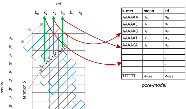
(a) Random accesses to the model array (red arrows) when kcache is not employed

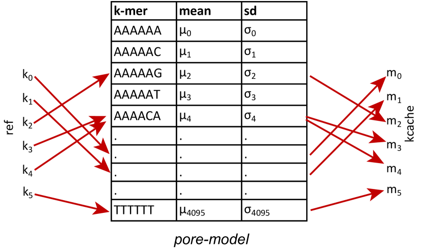
(b) Construction of the kcache in pre-kernel

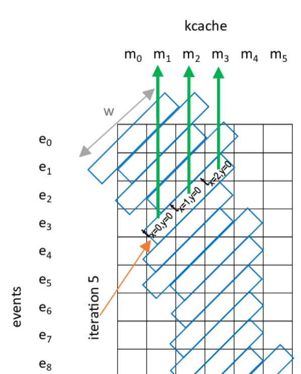
(c) Spatially local memory accesses (green arrows) when kcache is employed

Figure 5.7: Utility of kcache in the core-kernel to improve memory coalescing

Allocating one thread block per read (as in core-kernel to reduce warp divergence) is not ideal for this post-kernel due to the lack of fine grained parallelism (i.e. 1 block having 1 thread), which results in reduced GPU occupancy (occupancy will be limited by the maximum thread blocks that can simultaneously reside in a GPU multi-processor). This is remedied without affecting the warp divergence by allocating a large number of threads per block (eg: 1024) and then limiting only the first thread in the warp (a warp is composed of 32 contiguous threads [192] and thus thread with indices 0, 32, 64, 96 … etc) to perform the actual computation (backtracking for a read).

5.4.2 Memory optimisation

CPU version of the Adaptive Banded Event Alignment (ABEA) algorithm performs dynamic memory allocations (malloc) on a per read basis. The number of reads in a dataset is in the order of millions and thus incur millions of malloc calls. However, dynamic memory allocations (malloc performed inside GPU kernels) are extraordinarily expensive in terms of execution time [192]. In-fact, our initial GPU kernel implementation which performed such memory allocations was more than 100$\times$ slower than the CPU implementation. An intuitive approach of statically allocating memory at the compile time is not practical as nanopore read lengths vary significantly (~100 bases to >1 Mbases as explained previously) and thus the associated data structures vary from ~200 KB to >1.5 GB. We present a methodology that significantly reduces the number of memory allocations by pre-allocating large chunks of contiguous memory at the beginning of the program to accommodate a batch of reads, which are then reused throughout the life-time of the program. The sizes of these large chunks are determined by the available GPU memory and the average number of events per base (i.e. average value of the number of events divided the by the read length). For a given batch of reads, we assign reads to the GPU until the allocated GPU memory chunks saturate, and the rest of the reads are assigned to the CPU.

We describe the memory allocation technique in two steps: in Section 5.4.2.1 how the memory allocation for a batch of reads at a time is performed; and, in Section 5.4.2.2, how the method in Section 5.4.2.1 can be expanded to reuse large chunks of memory, allocated at the beginning of the program.

5.4.2.1 Data array serialisation

In the three GPU kernels elaborated in Section 5.4.1, the associated data arrays per each read are ref, kcache, events, score, trace, ll_idx and alignment (final output from the post-kernel). If any of these arrays are allocated inside the GPU kernels on a per-read basis, for instance if score and trace arrays are allocated at line 4 of Algorithm 12 using malloc), the performance will be degraded.

We identified that the sizes of all the aforementioned data arrays are dependent only on the read length (known at run-time during file reading) and the number of events for the read (known after event detection described in Section 5.2). Thus, the sum of read lengths and the number of events for a batch of $n$ reads (GPU processes a batch of $n$ reads at a time) is used to calculate the sizes of memory allocations required for the particular batch according to the formulation below.

Let $n$ be the number of reads loaded to the RAM (from the disk) at a time. Let $r[]$ be the read length and $e[]$ be the number of events for all the reads in batch of $n$ reads. Column 1 of Table 5.1, lists the data arrays. The size of arrays ref and kcache depends only on read lengths $r$; events and alignment depend on number of events $e$; and, score, trace and ll_idx depend on both read length $r$ and number of events $e$. Based on these dependencies, the arrays are categorised in Table 5.1 by horizontal separators. The second column of Table 5.1 states the data-type size of each array, denoted by constants of the form $c_{x}$. Typical values of these constants (in our implementation) are given inside the brackets. For instance, the data type for ref is char and thus $C_{r}$ is 1 byte. The data type for events is a struct of size $C_{e}$ that is 20 bytes. Note that, the exact values may depend on the implementation and the underlying processor architecture, nevertheless are constants known at compile time. The third column of Table 5.1 shows the size required for the particular array for a single read, i.e. the size for the i^th read (assume 0 based index origin) in the batch of $n$ reads. For instance, ref depends on the read length of the particular read and the datatype, thus the size is $C_{r}r[i]$. Score depends on read length, number of events, data type size and band-width ($W$), thus $WC_{s}(r[i]+e[i])$. The last column of Table 5.1 is the total size required for a batch of reads (based on sum of $r$ and $e$). For instance, the sum of all the ref arrays for the batch is the product of data type size $C_{r}$ and sum of all read lengths in the batch $\sum_{i=0}^{n-1}{r[i]}$.

Table 5.1: Data arrays associated with ABEA and their sizes

Array	Data type size	Size for read $i$ in batch	Size per batch
	(bytes)
ref[]	$C_{r}$ (1)	$C_{r}r[i]$	$C_{r}\sum_{i=0}^{n-1}{r[i]}$
kcache[]	$C_{k}$ (12)	$C_{k}r[i]$	$C_{k}\sum_{i=0}^{n-1}{r[i]}$
events[]	$C_{e}$ (20)	$C_{e}e[i]$	$C_{e}\sum_{i=0}^{n-1}{e[i]}$
alignment[]	$C_{a}$(8)	$2C_{a}e[i]$	$2C_{a}\sum_{i=0}^{n-1}{e[i]}$
score[][]	$C_{s}$ (4)	$WC_{s}(r[i]+e[i])$	$WC_{s}\sum_{i=0}^{n-1}{(r[i]+e[i])}$
trace[][]	$C_{t}$ (1)	$WC_{t}(r[i]+e[i])$	$WC_{t}\sum_{i=0}^{n-1}{(r[i]+e[i])}$
ll_idx[]	$C_{l}$(8)	$C_{l}(r[i]+e[i])$	$C_{l}\sum_{i=0}^{n-1}{(r[i]+e[i])}$

Based on the total array sizes in the last column Table 5.1, we can allocate seven big chunks of linear contiguous memory in the GPU. Let the base address of those chunks be represented by uppercase letters: REF; KCACHE; EVENTS etc. These memory allocations are performed using cudaMalloc() API calls, just before the kernel invocations and are deallocated after the kernels. Note that for now, we do these allocations and deallocations for each batch of reads.

The GPU arrays REF, KCACHE, EVENTS etc, allocated using cudaMalloc above are 1D arrays, thus multi-dimensional arrays in the RAM (eg: an array of pointers—each pointer pointing to a string/char array) must be serialised/flattened. One option is to save a series of pointers associated to each above array during the serialisation and then utilising those pointers for addressing a particular element later. However, this can be performed better by storing only two offset arrays of length $n$ each: read offset array $p[]$, which is the cumulative sum of read lengths in the batch ($p[i]=\sum_{j=0}^{i-1}{r[j]}$); and, event offset array $q$, which is the the cumulative sum of events in the batch ($q[i]=\sum_{j=0}^{i-1}{e[j]}$). Note that, $r$ and $e$ have the same definitions as before. These two offset arrays $p$ and $q$ can be used to deduce the associated pointer to a given element when required, by computing the array offset as shown in Table 5.2(a). The first column of Table 5.2(a) is the base address of the large GPU arrays we allocated above. The offset of the element pertaining to the i^th read (assume 0-indexing) in the particular array is given in the second column of Table 5.2(a). The definition of constants $C_{x}$ and $W$ are the same as for the previous Table 5.1. These 1D array base addresses in the first column of Table 5.2(a) and the two associated offset arrays $p[]$ and $q[]$, are passed as arguments to the GPU kernels (Algorithm 12 and Algorithm 13). These arguments are used for the the memory pointer computation inside the GPU kernels (line 4 of Algorithm 12 and line 4 of Algorithm 13) based on the second column of Table 5.2(a).

Table 5.2: GPU data arrays, pointer computation and heuristically determined sizes

(a) Computation of pointer for the read i

1D GPU array	Offset to element
(base address)	i in the batch
REF	$C_{r}p[i]$
KCACHE	$C_{k}p[i]$
EVENTS	$C_{e}q[i]$
ALIGNMENT	$2C_{a}q[i]$
SCORE	$WC_{s}(p[i]+q[i])$
TRACE	$WC_{t}(p[i]+q[i])$
LL_IDX	$C_{l}(p[i]+q[i])$

(b) Heuristic allocation

1D GPU array	Allocated size
(base address)	per batch
REF	$C_{r}X$
KCACHE	$C_{k}X$
EVENTS	$C_{e}Y$
ALIGNMENT	$2C_{a}Y$
SCORE	$WC_{s}(X+Y)$
TRACE	$WC_{t}(X+Y)$
LL_IDX	$C_{l}(X+Y)$

Algorithm 16 elaborates how the above mentioned strategy is integrated into the previous execution flow depicted in Algorithm 11. Lines 3-7 of Algorithm 16 show how the offset arrays $p$ and $q$ are computed for each batch of reads. Line 8 of Algorithm 16 performs the serialisation of the multi-dimensional arrays with the use of offset arrays $p$ and $q$. Line 9 of Algorithm 16 allocates GPU arrays based on sizes in last column of Table 5.1. Then, the serialised arrays are copied to allocated GPU memory (line 10 of Algorithm 16), GPU kernels (the three kernels discussed in Section 5.4.1) are executed (line 11) and the alignment result is copied back from the GPU (line 12). At the end, the alignment result is converted back to multi-dimesional arrays (line 13) and then the GPU memory (allocated at line 9) is deallocated (line 14).

The offset arrays $p$ and $q$ (and also REF, KCACHE, EVENTS, etc.) are passed onto the GPU kernels and are utilised inside the GPU kernels to compute the memory pointers (line 4 of Algorithms 12 and 13) through the equations listed on the second column of Table 5.2(a).

Algorithm 16 Memory allocation—data structure serialisation

1:for batch of $n$ reads do

2:     … $\triangleright$ CPU processing steps before the ABEA eg: event detection

3:     $rs,es\leftarrow 0,0$ $\triangleright$ cumulative sum of read lengths and no of events

4:     for each read $i$ do

5:         $p[i],q[i]\leftarrow rs,es$ $\triangleright$ save current read and event offsets

6:         $rs\leftarrow rs+r[i]$; $es\leftarrow es+e[i]$

7:     end for

8:     $serialise\_ram\_arays(p,q,...)$ $\triangleright$ flatten multi dimensional arrays in RAM to 1D arrays

9:     allocate_gpu_arrays(rs,es,…) $\triangleright$ GPU arrays REF, KCACHE, EVENTS, etc.

10:     $memcpy\_ram\_to\_gpu(...)$ $\triangleright$ copy inputs of the ABEA to the GPU memory

11:     $gpu\_alignment(p,q...)$ $\triangleright$ Perform ABEA on the GPU

12:     $memcpy\_gpu\_to\_ram(...)$ $\triangleright$ copy alignment result back to the RAM

13:     $deserialise(p,q,....)$ $\triangleright$ convert 1D result array to multi dimensional array

14:     $free\_gpu\_arrays()$ $\triangleright$ free GPU arrays REF, KCACHE, EVENTS, etc.

15:     … $\triangleright$ CPU processing steps after ABEA eg: HMM

16:end for

The limitation of this strategy is the GPU memory allocation and de-allocation (line 9 and 14 of Algorithm 16) performed for each batch of reads (which is expensive on certain GPUs, see Section 5.5.2.2). This limitation is remedied by the heuristic based pre-allocation strategy explained in the next subsection.

5.4.2.2 Heuristic based memory pre-allocation

The GPU memory allocations in the previous section which were performed for each batch could be eliminated by pre-allocating all the available GPU memory at the startup of the program and then re-using for subsequent batches of reads). If the sizes of the arrays depended only on the read length, the total read length accommodable into the available GPU memory can be derived. Then, the available memory can be allocated among the seven large arrays ($REF$, $KCACHE$, $EVENTS$ etc) in correct proportion. However, these array sizes depend both on the read length and the number of events which are unknown at the beginning of the program; thus, memory cannot be partitioned among the data arrays. Therefore, We present a heuristic approach which exploits characteristic of nanopore data to estimate the proportion to maximally utilise the available GPU memory. In summary, we obtain the average number of events per base (average of the number of events divided by read length), use this average to determine the maximum read length that can be accommodated to the GPU, and proportionally allocate the GPU arrays. This approach is formulated as follows.

Sum of all the cells in column 4 of Table 5.1 is total memory required for a batch of $n$ reads. This sum simplifies to equation 5.1 (due to the properties of constants) where $C_{R}=C_{r}+C_{k}+WC_{s}+WC_{t}+C_{l}$ and $C_{E}=C_{e}+2C_{a}+WC_{s}+WC_{t}+C_{l}$. This sum represents the total size of all array (for adapted banded event alignment algorithm) for a batch of $n$ reads.

$$S=C_{R}\sum_{i=0}^{n-1}{r[i]}+C_{E}\sum_{i=0}^{n-1}{e[i]}$$ (5.1)

If $\bar{\mu}$ is the average number of events per base (total number of events divided by the total read length for all reads in the batch), we can write as $\sum_{i=0}^{n-1}e[i]=\bar{\mu}\sum_{i=0}^{n-1}r[i]$. Now substituting this in equation 5.1 gives $S=(C_{R}+\bar{\mu}C_{E})\sum_{i=0}^{n-1}{r[i]}$. We observed that for a sufficient batch size (>64), $\bar{\mu}$ is stable ~2.5 (on more than 10 datasets we tested). Let this estimated value for $\bar{\mu}$ be represented by the constant $\mu$. Thus, the total memory required for a batch of reads can be estimated using equation 5.2.

$$M=(C_{R}+\mu C_{E})\sum_{i=0}^{n-1}{r[i]}$$ (5.2)

Equation 5.2 can be used to estimate the maximum number of bases (sum of read lengths) that a given amount of GPU memory can accommodate. Let $M$ in equation 5.2 be the available GPU memory. Then, the approximate maximum number of bases $X$ that fits available GPU memory $M$ can be computed via equation 5.3. Then, the associated total number of total events $Y$ which the GPU memory can accommodate, is found by equation 5.4.

$$X=floor\left(\frac{M}{C_{R}+\mu C_{E}}\right)$$ (5.3)

$$Y=floor(\mu X)$$ (5.4)

These $X$ and $Y$ allow the available GPU memory to be allocated among the seven large arrays ($REF$, $KCACHE$, $EVENTS$ etc) with approximately correct proportions, as shown in the second column of Table 5.2(b). The values in the second column of Table 5.2(b) are obtained by substituting $\sum_{i=0}^{n-1}{r[i]}$ with $X$ and $\sum_{i=0}^{n-1}{e[i]}$ with $Y$ in the last column of Table 5.1.

By incorporating the above heuristic based memory allocation strategy to Algorithm 16, we get the execution flow in Algorithm 17. The major changes to the previous Algorithm 16 are highlighted in blue text. Now the GPU memory is allocated at the beginning of the program based on the estimated $X$ and $Y$ on line 1 of Algorithm 17. As $X$ and $Y$ are approximations, the GPU arrays may saturate for certain batches of reads. Line 6 of Algorithm 17 checks if GPU arrays are saturated and assigns the read to either GPU (line 9) or CPU (line 11), accordingly. Only a few reads are assigned to the CPU and these few reads are processed on the CPU in parallel to the GPU kernel execution, and thus no additional execution time is incurred.

Algorithm 17 heuristic memory allocation scheme

1:allocate_gpu_arrays(X,Y) $\triangleright$ pre-allocate GPU arrays REF, KCACHE, EVENTS, etc.

2:for batch of $n$ reads do

3:     … $\triangleright$ CPU processing steps before the ABEA eg: event detection

4:     $rs,es\leftarrow 0,0$ $\triangleright$ cumulative sum of read lengths and no of events

5:     for each read $i$ do

6:         if  ($rs+r[i]\leq X$ and $es+e[i]\leq Y$) then $\triangleright$ check if GPU arrays have adequate free space

7:              $p[i],q[i]\leftarrow rs,es$ $\triangleright$ save current read and event offsets

8:              $rs\leftarrow rs+r[i];es\leftarrow es+e[i]$

9:              assign_to_gpu(i) $\triangleright$ GPU arrays have space, thus assign read to the GPU

10:         else

11:              assign_to_cpu(i) $\triangleright$ a GPU arrays is already full, thus assign the read to the CPU

12:         end if

13:     end for

14:     $serialise\_ram\_arays(p,q,...)$ $\triangleright$ flatten multi dimensional arrays in RAM to 1D arrays

15:     $memcpy\_ram\_to\_gpu(...)$ $\triangleright$ copy inputs of the ABEA to the GPU memory

16:     $gpu\_alignment(p,q...)$ $\triangleright$ Perform ABEA on the GPU

17:     process_rest_on_cpu() $\triangleright$ execute on the CPU in parallel to the GPU kernels

18:     $memcpy\_gpu\_to\_ram(...)$ $\triangleright$ copy alignment result back to the RAM

19:     $deserialise(p,q,....)$ $\triangleright$ convert 1D result array to multi dimensional array

20:     … $\triangleright$ CPU processing steps after ABEA eg: HMM

21:end for

22:free_gpu_arrays() $\triangleright$ free GPU arrays REF, KCACHE, EVENTS, etc.

Note: Changes to Algorithm 16 are highlighted in blue

With the heuristic based memory pre-allocation strategy described in this section, cudaMalloc operations are invoked only at the beginning of the program and thus no additional memory allocation overhead during the processing. Note that, our implementation is future proof; i.e. $\mu$ is a user specified parameter (that is initialised to 2.5 by default) in case nanopore data characteristics change in future.

5.4.3 Heterogeneous processing

If all the reads were of similar length, GPU threads that process the reads would complete approximately at the same time, and thus GPU cores will be busy throughout the execution. However, as stated in Section 5.2, there can be a few reads which are significantly longer than the other reads (we will refer to them as very long reads). When the GPU threads process reads in parallel, presence of such very long reads will cause all other GPU threads to wait until the GPU threads processing the longest read complete. This thread waiting leads to under utilisation of GPU cores. Thus, we process these very long reads on the CPU while the GPU is processing the rest in parallel. However, there can be exceptionally long reads (we will refer to them as ultra long reads) which the CPU would take longer time than what the GPU took to process the whole batch. Such reads would lead the GPU to idle until the CPU completes. Thus, ultra long reads will be skipped and will be processed separately at the end by the CPU. Similarly, there can be a few over segmented reads (i.e. reads with a significantly higher events per base ratio than the others) which cause GPU under utilisation. These over-segmented reads will also be processed on the CPU.

We discuss these problems of very long reads and ultra long reads in detail with examples in Section 5.4.3.1, along with the solutions. Then, in this Section 5.4.3.2, we discuss the problem of over segmented reads and the respective solution. Then, in Section 5.4.3.3, we discuss another factor that affects performance, the batch size (number of reads loaded to the RAM at a time). Finally, in Section 5.4.3.4, we describe a method to detect and prompt the user of any drastic impacts on performance along with suggestions to tune parameters to minimise the impact.

5.4.3.1 Very long reads and ultra long reads

Consider a batch of reads where ~90% of the reads are less than 30 Kbases in length. Assume the longest read in the batch is 90 Kbases. Assume that the GPU is processing all the reads (in the batch) in parallel. Suppose that GPU threads processing reads of length <30 Kbases (90% of the threads) would complete in <300ms while GPU threads processing the longest 90 Kbases read would take 900ms. As a result, the completed GPU threads will have to wait for additional 600ms. Similarly, the few very long reads consume a significant time to process on the GPU in comparison to other reads in the batch. Majority of the GPU threads will have to wait and this causes under-utilisation of GPU compute-cores. Furthermore, very long reads negatively affects the GPU occupancy by occupying a significant portion of GPU memory. For instance, a read of size ~10 Kbases requires only ~18 MB of GPU memory while a read with 90 Kbases requires ~160MB memory. Hence, very long reads occupy a significant portion of GPU memory, limits the number of reads that could be processed in parallel. This reduces the amount of parallelism and the occupancy of the GPU is reduced.

Fortunately, very long reads being few (see the typical read length distribution under results), the CPU (core frequency faster than on GPU) could process those reads while GPU is processing the rest of the reads. In the above example, selecting a static threshold (eg: processing reads of length <30Kbases on GPU and rest on CPU) would give reasonable performance. However, selecting such a static threshold is not ideal due to variations in the read length distributions based on the dataset (see background). Thus, we use the product of max-lf and the average read length in the batch to determine the threshold dynamically, where max-lf is a user-parameter that defaults to 5.0. This threshold was empirically determined.

Now assume amongst the very long reads processed on the CPU, a few ultra long reads (eg: read >100 Kbases in a dataset where >99% of the reads are <100 Kbases). Such ultra long reads could cause a severe load imbalance between the CPU and the GPU. For instance, assume that there exists a read which is 1 Mbases in a given read batch. Despite the high core frequency, the CPU will take a few seconds to process such an ultra long read. The GPU meanwhile would process the whole batch in less than 1s (see results for empirical evidence). Such ultra long reads being <1%, are skipped during the processing (while being written to a separate file) and are separately processed by the CPU at the end. In our implementation, the threshold for ultra long reads is a user defined parameter which defaults to 100 Kbases. There is an additional advantage of processing ultra long reads later. Ultra long reads usually require a significant amount of RAM (a few gigabytes) and may crash on limited memory systems. In the end, it is possible to process these reads with a limited amount of threads to reduce the peak memory consumption, particularly if the size of the RAM is limited.

5.4.3.2 Over segmented reads

Once the very long reads and ultra long reads are processed as in Section 5.4.3.1, the performance impact due to the over-segmented events become prominent. While majority of the reads have a number of events per base that is close to the average $\mu(=2.5)$, a few reads can have a very large value. For instance, a few reads with a number of events per base being more than eight times the average $\mu(=2.5)$ can violate the suitability of our partitioning of GPU memory as $X$ and $Y$ ($X$ and $Y$ are derived in equations 5.3 and 5.4). These over-segmented reads lead to the GPU arrays that are proportional to $Y$ be full, while the arrays proportional to $X$ are left under-utilised. For instance, arrays proportional to $Y$ can become 100% while arrays proportional to $X$ are only filled to <70%. Hence, over segmented reads lead to under-utilisation of GPU memory and results in limiting the number of reads which are processed in parallel. We process the over-segmented reads on the CPU based on a user specifiable threshold max-epk which defaults to 5.0.

On rare occasions, reads with >100 events per base were observed. Such severely over-segmented reads can be processed separately at the end or ignored totally as such rare reads amongst millions of other reads are unlikely to affect the final polishing result.

5.4.3.3 Batch size

Selection of proper batch size (reads loaded to RAM from the disk at a time) is another important parameter that affects performance. If the batch size is too small compared to what the GPU memory can accommodate, the number of reads to be processed in parallel is limited, thus leads to in-adequate occupancy. Conversely, if the batch is too large to fit the GPU, CPU will have to process many surplus reads that could not be accommodated into the GPU. The batch size in our implementation is determined by two user specified parameters: $K$ which is the maximum number of reads; and, $B$ which is the maximum number of total bases. When reading from the disk to RAM, the true batch size ($n$-number of reads and $b$-number of total bases are capped by $K$ and $B$) is determined by the first value ($n$ or $b$) reaching the cap ($K$ or $B$) first. Having such a limit $B$ allows to cap peak RAM due to adjacent very long reads. The suitable value for $B$ is dependent on the available GPU memory, which can be estimated via the equation 5.3 discussed in Section 5.4.2.

5.4.3.4 Detection of performance anomalies

While we have empirically determined typical parameters/thresholds (associated with above strategies), an unusual situation (for instance, a big gap between the CPU and GPU specifications or a data set that severely deviates from the heuristics we use) may cause performance anomalies. We employ the following method to detect a severe performance anomaly caused by such an unusual scenario.

We measure the quantities representing resource utilisation during run time, which are listed in Table 5.3. These quantities are measured per batch of reads loaded to the RAM at a time. We use those measured quantities to determine any severe performance issues and suggest suitable parameter adjustments to the user. The adjustable parameters (or thresholds) that can be tweaked to improve the resource utilisation are defined in Table 5.4. Determination of performance issues and suggestions are done via two decision trees, one that corresponds to GPU memory usage (Fig. 5.8(a)) and another which corresponds to balancing the load between CPU and GPU (Fig. 5.8(b)).

quantity	description
tCPU	processing time on CPU
tGPU	processing time on GPU
Xutil	utilisation percentage of the arrays proportional to $X$ (rs as a percentage of $X$ in Algorithm 17)
Yutil	utilisation percentage of the arrays proportional to $Y$ (es as a percentage of $Y$ in Algorithm 17)
Nmemout	number of reads assigned to CPU due to GPU memory getting prematurely full (corresponds to line 11 of Algorithm 17)
Nlong	number of very long reads assigned on to the CPU (corresponds to user parameter max-lf)
Nevents	number of reads with too many events per read assigned onto the the CPU (corresponds to user parameter max-epk)
$n$	the number of reads actually loaded to the RAM
$b$	the number of bases actually loaded to the RAM

Table 5.3: measured quantities

parameter	description
max-lf	reads with length $\leq$ max-lf $\times$ average_read_length are assigned to GPU and rest to CPU
avg-epk	average number of events per base used for allocating GPU arrays as discussed previously ($\mu$)
max-epk	reads with events per base $\leq$ max-epk are assigned to GPU, rest to CPU
$K$	upper limit of the batch size with respect to the number of reads
$B$	upper limit of the batch size with respect to the number of bases
$t$	number of CPU threads
ultra-thresh	threshold to skip ultra long reads

Table 5.4: adjustable user parameters

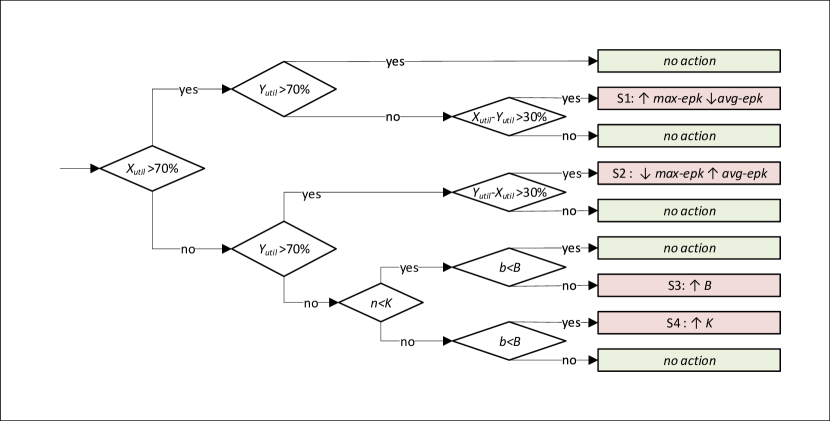
(a) memory balancing

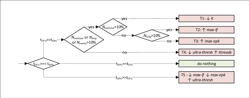
(b) load balancing

Figure 5.8: Decision trees for resource optimisation

Fig. 5.8(a) shows the decision tree that detects any imbalance in the proportions $X$ and $Y$ associated with GPU arrays allocation ($X$ and $Y$ derived in equations 5.3 and 5.4). The objective of this decision tree is to detect any GPU memory wastage and to increase the number of reads which the GPU gets to process in parallel.

As shown in Fig. 5.8(a), if both $X_{util}$ and $Y_{util}$ (rs as a percentage of $X$ and es as a percentage of $Y$ in Algorithm 17) are more than 70%, the utilisation of GPU arrays is considered reasonable. Note that 70% is an empirically determined value that provides adequate performance. If $X_{util}$ is reasonable (>70%) and $Y_{util}$ is unreasonable (<70%), we inspect for any significant imbalance between $X_{util}$ and $Y_{util}$ ($X_{util}$-$Y_{util}$>30%). Such a significant gap suggests an under-utilisation, which should be remedied through the increase of max-epk (the threshold at which over-segmented reads are offloaded to the CPU) or reducing Y by decreasing average-epk (node S1 in Fig. 5.8(a)). In contrast, if $Y_{util}$ is reasonable and the $X_{util}$ is unreasonable, the strategy is the opposite, i.e, either decrease max-epk or increase average-epk (follow up to the node S2 in Fig. 5.8(a)).

If both $X_{util}$ and $Y_{util}$ are less than 70%, a likely cause is an inadequate batch size to fill the GPU memory. The actual batch size ($n$,$b$) is determined by both $K$ and $B$ as stated previously. As shown in Fig. 5.8(a), we check which limit out of $K$ and $B$ was reached first. If both $n<K$ and $b<K$, the currently processed batch being the last batch in the dataset (end of input data reached) is the likely cause. Thus, no parameter tuning action is necessary. If $B$ was reached first ($n<K$ and not $b<B$), $B$ is the limitation and should be increased (S3 in Fig. 5.8(a)). If $K$ was reached first (not $n<K$ and $b<B$), $K$ should be increased (S4 in Fig. 5.8(a)).

Fig. 5.8(b) shows the decision tree for CPU-GPU workload balancing. For a particular batch, if the CPU takes significantly more time than the GPU, the decision tree first inspects whether the CPU is assigned with an excessive workload. An excessive workload on the CPU can be attributed by: an extensively over-sized batch size (in comparison to the available GPU memory), which results in a majority of the reads being assigned to the CPU (N_memout>10%); excessive number of very long reads assigned to the CPU (N_long>10%); and, excessive number of over-segmented reads events assigned to the CPU (N_events>10%). If N_memout>10%, $K$ is reduced (node T1 in Fig. 5.8(b)); if N_long>10%, max-lf is increased (T2 in Fig. 5.8(b)); and, if N_events>10%, max-epk is increased (T3 in Fig. 5.8(b)).

If the cause for higher CPU time is not the aforementioned excessive workload, a likely cause is ultra long reads, where a single ultra long reads processed on the CPU taking more time than the time taken by GPU for the whole batch. In such an event, ultra-thresh threshold is reduced so that more ultra long reads are skipped. Another likely cause is that the program was executed with inadequate threads (if the CPU had more hardware threads than the program was launched), which is to be remedied by increasing the number of CPU threads. Another cause might be that the CPU is not sufficiently powerful to match with the GPU and thus no action can be taken (except upgrading the CPU). These actions are denoted by T4 in Fig. 5.8(b).

The ideal case is when the CPU and GPU take similar times which requires no intervention.

Conversely, if the GPU takes significant time than the CPU, the likely causes are very long reads or over-segmented reads. In such event, the thresholds max-lf and max-epk are decreased so that more very long reads and over-segmented reads are assigned to the CPU. Another likely cause is the ultra long read which can be remedied by increasing ultra-thresh threshold. Another cause might be an insufficiently powerful GPU (less compute cores or less memory) compared to the CPU and no action is taken (except to upgrade the GPU).

To reduce false positives due to incidental under utilisation, a suggestion is provided to the user, only if the same condition (condition that led to the decision in the decision tree, S1 to S4 T1 in Fig. 5.8(a) and T1 to T4 in Fig. 5.8(b)) consecutively repeats more than a few times (eg: >3 times).

Note that the above mentioned strategy is to warn and suggest of potential parameter adjustments in the event of drastic performance degradation, rather than to obtain optimal performance or to determine the exact parameter values.

5.5 Results

Experimental setup is given in Section 5.5.1. In Section 5.5.2, we present experimental evidence that justify the selection of steps presented in Section 5.4. Next in Section 5.5.3, we compare the GPU implementation of the Adaptive Banded Event Alignment (ABEA) algorithm to its CPU implementation. Finally, we show the overall speedup of the GPU implementation when incorporated into an actual work-flow (i.e. detection of methylated bases).

5.5.1 Experimental setup

We re-engineered the Nanopolish methylation calling tool (existing methylation detection tool discussed in Section 5.2) to: one, load a batch of n reads from disk to RAM at a time, instead of on-demand loading; two, synchronise CPU threads prior to GPU kernel invocation (Nanopolish assigns a thread dynamically to a particular thread, thus each read follows its own code path); and three, optimise the CPU implementation which otherwise would result in an apparent un-fair speedup (when the optimised GPU version is compared to an un-optimised CPU version). Re-engineered Nanopolish employs a fork-join multi-threading model (with work stealing) implemented using C POSIX threads. ABEA algorithm for the GPU was implemented using CUDA C. This re-engineered Nanopolish will be hitherto referred to as f5c.

We used publicly available NA12878 (human genome) Nanopore WGS Consortium sequencing data [56] for the experiments. The datasets used for the experiments, their statistics (number of reads, total bases, mean read length and maximum read length) and their source are listed in Table 5.5. D_small which is a small subset, is used for running on a wide range of systems (all systems in Table 5.6: embedded system, low-end and high-end laptops, workstation and high-performance server). Two complete MinION data sets (D_ligation and D_rapid) are only tested on three systems due to large run-time and incidental access to the other two systems. D_ligation and D_rapid represent the two existing nanopore sample preparation methods (ligation and rapid [199]) that affects the read length distribution.

Table 5.5: Information of the datasets

Dataset	Number of reads	Number of bases (Gbases)	Mean read length (Kbases)	Max read length (Kbases)	Source / SRA accession
Dsmall	19275	0.15	7.7	196	[200]
Dligation	451020	3.62	8.0	1500	ERR2184733
Drapid	270189	2.73	10.0	386	ERR2184734

Table 5.6: Different systems used for experiments

System Name	Info	CPU	CPU cores / threads	RAM (GB)	GPU	GPU mem (GB)	GPU arch
SoC	NVIDIA Jetson TX2 embedded module	ARMv8 Cortex-A57 + NVIDIA Denver2	6 / 6	8	Tegra	shared with RAM	Pascal / 6.2
lapL	Acer F5-573G laptop	i7-7500U	2/4	8	Gefore 940M	4	Maxwell / 5.0
lapH	Dell XPS 15 laptop	i7-8750H	6/12	16	Gefore 1050 Ti	4	Pascal / 6.1
ws	HP Z640 workstation	Xeon E5-1630	4/8	32	Tesla K40	12	Kepler / 3.5
HPC	Dell PowerEdge C4140	Xeon Silver 4114	20/40	376	Tesla V100	16	Volta / 7.0

D_small dataset was used for experiments under Sections 5.5.2.2, 5.5.2.1 and 5.5.3.1. For experiments under Sections 5.5.3.2 and 5.5.4, the datasets D_rapid and D_ligation were used.

To obtain the results for Section 5.5.2.3, first we grouped the reads in dataset D_rapid based on their read lengths. We grouped the read into 10 Kbases bins (i.e., 0K-10K,10K-20K…90K-100K). Reads with >100 Kbases were grouped into larger bins (100K bin sizes; 100K-200K, 200K-300K and 200K-300K) as the read count is very little in the range that certain 10K bins would contain no reads at all. Then, we ran f5c with only CPU and f5c with GPU acceleration on each group of the reads separately. Then, we computed the speedup of ABEA for each group of reads: the kernel only speedup (GPU kernel time / time on CPU); and, the speedup with overheads (overheads such as memory copy, data structure serialisation). This experiment was performed on the system lapH.

For Sections 5.5.2 and 5.5.3, time measurements were obtained by inserting gettimeofday function invocations directly into the C source code. Total execution time and the peak RAM usage in Section 5.5.4 were measured by running the GNU time utility with the verbose option.

5.5.2 Effect of individual optimisations

5.5.2.1 Compute optimisations

Fig. 5.9(a) shows the time consumed by the three GPU kernels after applying the compute optimisation techniques discussed in Section 5.4.1. Time taken by each of the three GPU kernels (pre-kernel, core-kernel and post-kernel) is plotted for each different GPU. It is observed that the core-kernel, which computes the dynamic programming table (compute-intensive portion), still consumes the majority of the GPU compute time. The pre-kernel which performs data structure initialisation consumes much lesser time and shows that there is no need to further parallelise the loop in Algorithm 12 (explained in Section 5.4.1). Despite the lack of fine-grained parallelism in post-kernel (which performs backtracking), the elapsed time is still considerably lesser than the core-kernel. Thus, any future optimisations should still mainly focus on the core-kernel, followed by the post-kernel.

The efficacy of our compute optimisations on the compute intensive core-kernel can be elaborated using the reported statistics from the NVIDIA profiler (instruction level profiling—PC sampling in NVIDIA visual profiler [201]). The profiler reports the percentage distribution of reasons that caused the thread warps to stall, based on the number of clock cycles. The percentage of the number of clock cycles that a warp was stalled due to a memory dependency (waiting for a previous memory accesses to complete), improved from 59.10% to 44.81% after the use of GPU shared memory. After exploiting the kcache for improving memory coalescing, this percentage further improved to 28.62%.

5.5.2.2 Memory optimisations

As stated in Section 5.4.2.1, the data array serialisation technique eliminated all memory allocations inside GPU kernels (malloc); still, required memory allocations per each batch of reads (cudaMalloc). The overhead due to these cudaMalloc calls are plotted in Fig. 5.9(b) along with the time for kernel execution and data transfer to/from the GPU (using cudaMemcpy). Observe that on certain GPUs (Jetson TX2, GeForce 940M and Tesla K40), the overheads due to cudaMalloc operations are significant in comparison to the compute kernels (even higher than the compute kernels in Jetson TX2). Such significant overheads justify why we proposed a heuristic based memory pre-allocation technique (Section 5.4.2.2) which completely eliminates this overhead.

Interestingly, Tesla K40 and Gefore 940M which incurred high cudaMalloc overheads are of relatively older GPU architectures in comparison to GeForce 1050 and Tesla V100, where the overheads were minimal. This is probably due to hardware supported memory allocation in latest GPU architectures. However, the aforementioned observation seems to be valid only for GeForce GPUs (targeted for gaming on PC/laptops) and Tesla GPUs (targeted for high performance computing). On Tegra GPUs (SoC targeted for embedded devices) the overhead seems to be significant in spite of the latest architectures (Jetson TX2 is the same Pascal architecture as GeForce 1050). We additionally tested on a Jetson AGX Xavier (the most recent Tegra GPU based SoC — Volta architecture) and cudaMalloc was yet expensive (40s on GPU kernels and 44s on cudaMalloc, not shown in figure). Thus, our memory pre-allocation strategy (in Section 5.4.2.2) which totally eliminates this cudaMalloc overhead is specifically beneficial for GPU on SoCs.

5.5.2.3 Heterogeneous processing

We stated in Section 5.4.3 that very long reads if processed on the GPU, limits the GPU occupancy. Fig. 5.9(c) provides experimental evidence and shows the need to process very long reads on CPU (explained in Section 5.4.3). Fig. 5.9(c) plots the variation of the speedup (GPU compared to CPU for ABEA) as the read length varies. The x-axis labels the range of the read length for which the speedup was computed (explained in the experimental setup). For instance, 0-10 on the x-axis refers to the group of reads with read length 0-10Kbases. Note that in Fig. 5.9(c) the bins are 100K wide from 100K-200K on-wards, due to less number of reads of those lengths (explained in the experimental setup). The speedup of computations (GPU kernel time / CPU time) and the speedup including overheads (GPU kernel time + overheads such as memory copy, data structure serialisation) are plotted in Fig. 5.9(c). Speedup of more than 4X was observed for smaller read lengths (0-10K). speedup drops with increasing read-length and is less than 3X from 50K-60K. The longer the reads are, the lesser number of reads can be processed in the GPU in parallel (reduced occupancy), thus the reduced speedup. Hence, very long reads that significantly affects the performance should be performed on the CPU while the GPU is processing the rest.

Fig. 5.9(d) shows the need for processing ultra long reads separately (explained in Section 5.4.3). The x-axis in the figure is the read-length (similar to Fig. 5.9(c)). The blue bars (with reference to the right y-axis) denote the average time consumed by the GPU to process a batch of reads (1.5 Mbases), for each group of read lengths from 0 bases to 50Kbases. The orange bars (with reference to the right y-axis) denote the average time consumed by the CPU (1 thread) to process a single read in the particular group of reads. The read length distribution (left y-axis) is shown shaded in green colour to depict the abundance of reads in each read length. Observe that CPU takes >1.6s for a single read of 300K-400K length while the GPU completes a whole 40K-50K batch in <0.4s. Thus, the GPU would idle for >1.2s until the CPU completes processing. Hence, such ultra long reads (eg : >100 Kbases) must be skipped and processed separately at the end. Note that such ultra long reads are very few (green coloured read length distribution in Fig. 5.9(d)).

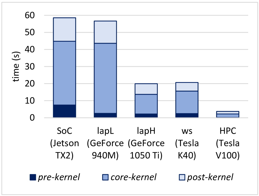
(a) Distribution of GPU kernel execution time

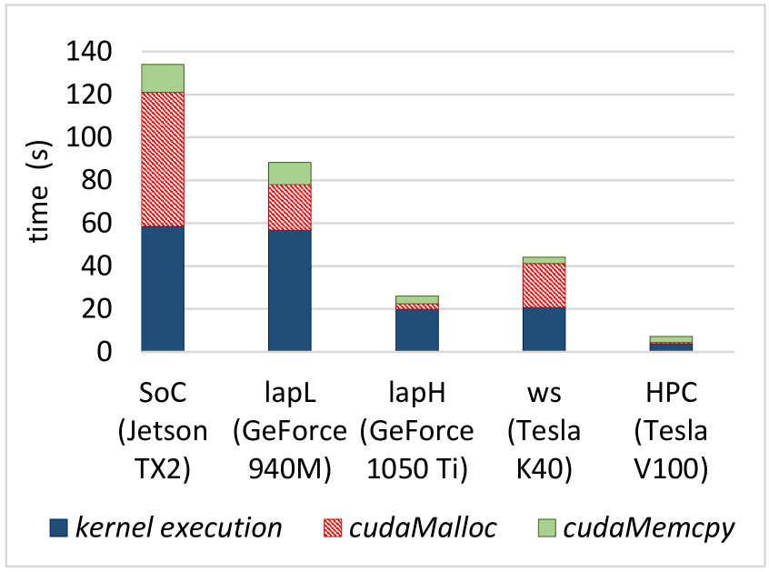
(b) Time for GPU kernels compared cudaMalloc

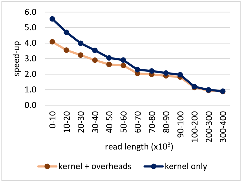
(c) Effect of the read length on the speedup

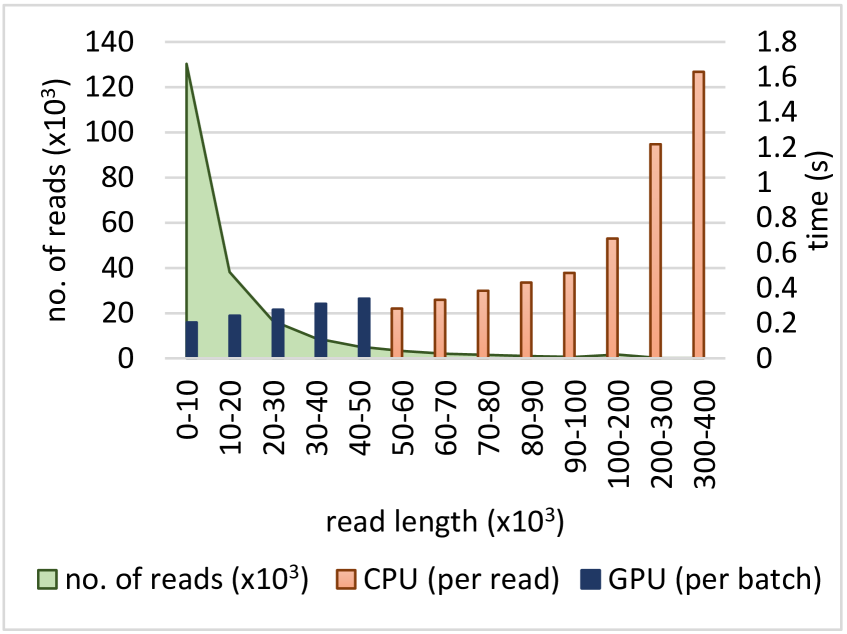
(d) need for load-balancing based on read lengths

Figure 5.9: Effect of individual optimisations

5.5.3 Speedup of Adaptive Banded Event Alignment

In this subsection, we present the performance of the GPU ABEA implementation when all the optimisations in Section 5.4 are applied together. Note that we compare this optimised GPU version with optimised CPU version in f5c (not the CPU version in original Nanopolish). The CPU version was run with maximum supported threads on the system. The optimised CPU version will be hitherto referred to as CPU-opti and the optimised GPU version will be referred to as GPU-opti. First, we compare the run-time of CPU-opti and GPU-opti on a wide range of different computer systems in Section 5.5.3.1, and then on the two big datasets in Section 5.5.3.2.

5.5.3.1 Across different devices

Fig. 5.10(a) shows the time for CPU-opti (left bars) and the GPU-opti (right bars) for the Dataset D_small, for each system listed in Table 5.6. The run-time for the GPU has been broken down in to: compute kernel time; different overheads (memory copying to/from the GPU, data serialisation time); and, the extra CPU time due to reads processed in the CPU. The compute kernel time includes the sum of time for all the three kernels (pre-kernel, core-kernel and post-kernel). The extra CPU time is the additional time spent by the CPU to process the reads assigned to the CPU (excluding the processing time that overlaps with the GPU execution, i.e. only the extra time which the GPU has to wait after the execution is included). Note that the ultra long reads were not separately processed on the CPU as the D_small contains a minuscule number of ultra long reads.

Speedups (including all the overheads) observed for CPU-opti compared to GPU-opti are: ~4.5$\times$ on the low-end-laptop and the workstation; ~4$\times$ on Jetson TX2 SoC; and ~3$\times$ on high-end-laptop and HPC. Note that only ~3$\times$ speedup on high-end-laptop and HPC (in comparison to >=4$\times$ on other systems) is due to the CPU on those particular systems having comparatively a higher number of CPU threads (12 and 40 respectively).

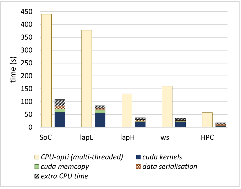
(a) Performance comparison of ABEA on CPU vs GPU for D_small over a wide range of systems

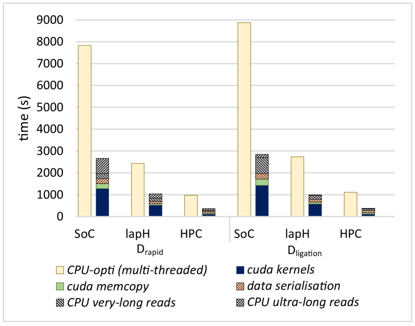
(b) Performance comparison of ABEA on CPU vs GPU across full datasets

Figure 5.10: Speedup of ABEA on GPU compared to CPU

5.5.3.2 Benchmark on big datasets

Time taken for CPU-opti compared to GPU-opti for the two big datasets (D_ligation and D_rapid) is shown in Fig. 5.10(b). Experiments were performed only on three systems due to the limited availability of other devices (mentioned previously). The graph is similar to the previous Fig. 5.10(a), except the extra CPU time has been further broken down to: CPU very-long reads; and, CPU ultra long reads. CPU very long reads refers to the additional time spent by the CPU to process very long reads and, CPU ultra long reads refer to the ultra long reads (reads >100 Kbases) processing time performed separately on the CPU. A speedup up of ~3$\times$ was observed for all three systems. Due to more ultra long reads in D_ligation and D_rapid than in D_small, the overall speedup for SoC is limited to around ~3$\times$ compared to ~4$\times$ for D_small.

5.5.4 Total run-time of f5c compared with original Nanopolish

In this section, we demonstrate the overall performance when the GPU accelerated ABEA is incorporated into an actual methylation detection work-flow. As stated in the experimental setup, we re-engineered Nanopolish to overcome the limitations of original Nanopolish. We compare the total run-time for methylation calling using original Nanopolish against f5c (both CPU only and GPU accelerated versions).

We refer to original Nanopolish (version 0.9) as nanopolish-unopti, f5c run only on the CPU as f5c-cpu-opti and GPU accelerated f5c as f5c-gpu-opti. We executed nanopolish-unopti, f5c-cpu-opti and f5c-gpu-opti for the full datasets D_rapid and D_ligation. Note that all the executions were performed with the maximum number of CPU threads supported on each system.

The run-time results are shown in Fig. 5.11. The reported run-times are for the whole methylation calling (all steps mentioned in Section 5.2.2) and also includes disk I/O time. As each read executes on its own code path in original Nanopolish (as mentioned in the experimental setup) the time for individual components (eg: ABEA) cannot be accurately measured, thus we only compare the total run-times.

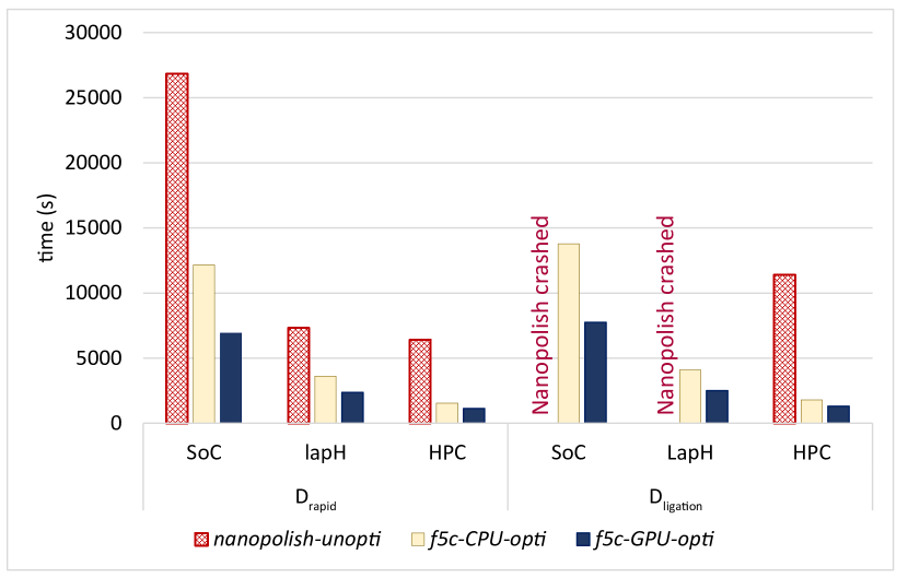
Figure 5.11: Comparison of f5c to Nanopolish

f5c-cpu-opti for D_rapid dataset was: ~2$\times$ faster on SoC and lapH; and, ~4$\times$ faster on HPC. nanopolish-unopti crashed on SoC (8GB RAM) and lapH (16GB RAM) when run for D_ligation dataset due to Linux Out Of Memory (OOM) killer [202]. When run for D_ligation on HPC, f5c-cpu-opti was not only 6$\times$ faster than original Nanopolish, but also consumed only ~15 GB RAM opposed to >100 GB by original Nanopolish (both run with 40 threads). Hence, it is evident that CPU optimisations alone can do significant improvements.

As per Fig. 5.11 for the whole methylation-calling process (including disk I/O), f5c-gpu-opti (only ABEA is performed on GPU) compared to f5c-cpu-opti was 1.7$\times$ faster on SoC, 1.5-1.6$\times$ on the lapH and <1.4$\times$ on HPC. On HPC the speedup was limited to <1.4$\times$ due to file I/O being the bottleneck.

When the execution time of f5c-gpu-opti for D_rapid is compared with original Nanopolish, it is ~4$\times$, ~3$\times$ and ~6$\times$ faster on SoC, laptop and HPC, respectively. On HPC for D_ligation, f5c-gpu-opti was ~9$\times$ faster.

Note that we used Nanopolish v0.9 for comparison as the re-engineering was done on this particular version. As we incorporated a number of CPU optimisations identified during the re-engineering into the subsequent version of Nanopolish (only those that did not require major code refactoring), latest Nanopolish v0.11 should be faster than v0.9 used in this paper.

5.6 Discussion

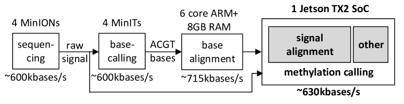
Figure 5.12: Human genome processing on-the-fly

With the method discussed in this paper, the complete methylation calling of a human genome can now be performed on-the-fly (process in real-time while the nanopore sequencer is operating) on an embedded system (e.g., an SoC equipped with ARM processor and an NVIDIA GPU) as shown in Fig. 5.12 (four Oxford Nanopore MinION devices sequencing in parallel or a single Oxford Nanopore GridION, is capable of sequencing a human genome at an adequate coverage). f5c powered by GPU accelerated ABEA can process the output from the rest of the pipeline on a single NVIDIA TX2 SoC, at a speed of (>600 Kbases per second) to keep up with the sequencing output (~600 Kbases per second [196]) as shown in Fig. 5.12. Conversely, if the original Nanopolish was executed on the NVIDIA TX2 SoC, the processing speed is limited to ~256 Kbases per second. Our work will not only reduce the associated costs of Nanopore data processing and data transfer, but will also improve turnaround time of the final test outcome.

In addition to embedded systems, our work benefits systems with or without GPU. Due to reduced peak memory usage, methylation calling can be performed on laptops with <16GB of RAM. Furthermore, post sequencing methylation calling execution on high performance computers also benefit from a significant speedup in processing.

A limitation of our implementation is that the parameter tuning cannot be performed automatically, which instead prompts the user when an un-optimal parameter is detected. This limitation is expected to be addressed in a future version by automatically tuning the parameters at run-time; or, by the use of pre-set parameter profiles for different types of datasets and/or computer systems.

The documentation of f5c is in appendix B. Supplementary material on the design, development and deployment of f5c is available in appendix C and appendix D.

5.7 Summary

Adaptive Banded Event Alignment algorithm is one of the key components in nanopore data analysis. Despite this algorithm being not embarrassingly parallel, we presented an approach that makes this algorithm efficiently execute on GPUs. The high variability of the read lengths was one of the main challenges, which was remedied through a number of memory optimisations and a heterogeneous processing strategy that uses both CPU and GPU. Our optimisations yield around 3-5$\times$ performance improvement on a CPU-GPU system when compared to a CPU. We incorporated the optimised Adaptive Banded Event Alignment algorithm into a methylation detection workflow and demonstrated that an embedded SoC equipped with an ARM processor (with six cores) and NVIDIA GPU (256 cores) is adequate to process data from a portable nanopore sequencer in real-time.

This work not only benefits embedded SoC, but also a wide range of systems equipped with GPUs from laptops to servers. The re-engineered version of the Nanopolish methylation detection module, f5c that employs the GPU accelerated Adaptive Banded Event Alignment was not only around 9$\times$ faster on an HPC, but also reduced the peak RAM by around 6$\times$ times. The source code of f5c is made available at https://github.com/hasindu2008/f5c.

Chapter 6 System Integration

6.1 Introduction

This chapter presents how the different optimisations proposed in previous chapters are integrated to construct different prototype embedded systems that perform end-to-end DNA analysis workflows.

In collaboration with two other PhD candidates in the research group, an embedded system called SWARAM was constructed for performing a variant calling pipeline for second-generation sequencing. SWARAM consisted of 16 Odroid XU4 single board computers (SBC) interconnected through Ethernet. The optimisations to the Platypus variant caller presented in chapter 3 are applied in SWARAM to facilitate fast variant calling. However, the integration details and the architecture of SWARAM have been generously shared to be used in another PhD candidate’s thesis and thus not discussed or claimed under this thesis. Refer to the published article at [27] for those details.

Inspired by SWARAM, another embedded system called the nanopore-cluster was constructed, now in a different architecture to SWARAM, to process third-generation nanopore sequencing data. The optimisations proposed in chapter 4 and 5 were used in this nanopore-cluster to enable a real-time workflow for nanopore sequencing data. As mentioned in section 2.1.2.3, nanopore is a highly portable technology. Thus, an embedded like the nanopore-cluster system is harmonious with the ultimate goal of such ultra-portable sequencers to enable complete DNA sequencing in-the-field. Further, unlike second generation Illumina sequencers, third-generation nanopore sequencers allows streaming and thus the processing can be performed while sequencing. This streaming capability can be exploited in an embedded system like the nanopore-cluster, to perform data analysis on-the-fly while the sequencer is operating, intending to produce the result soon after the sequencing run is completed.

6.2 System Architecture of Nanopore-cluster

6.2.1 Hardware Architecture

The hardware architecture of the proposed system is in Fig. 6.1. The system comprised of the DNA Sequencer and the base-caller, Network Attached Storage (NAS) and the computational nodes (head node and the worker nodes) are interconnected using Ethernet via a layer 2 Switch. The system is interfaced with the Internet or the Intranet through a router (layer 3 switch) supporting Network Address Translation (NAT). The function and details of individual components are elaborated below:

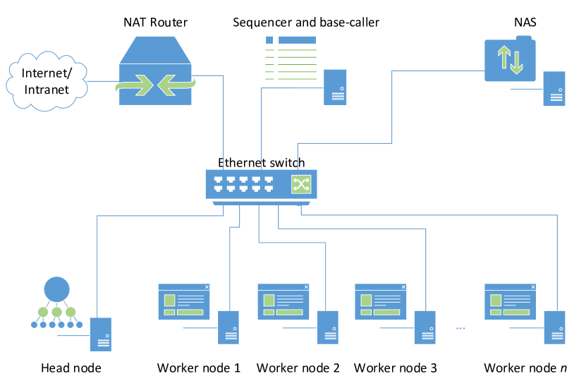
Figure 6.1: Hardware architecture of the proposed system

Sequencer and base-caller: The sequencer can be one of the available nanopore sequencers - MinION, GridION or PromethION (Fig. 2.10). If the sequencer is a MinION or a PromethION, it must be connected to the corresponding base-calling unit (to the MinIT in case of the MinION or the compute tower in case of the PromethION; see Fig. 2.11). It is this base-calling unit that is connected to the Ethernet switch through the available Ethernet interface on the case-calling unit. If the sequencer is a GridION or a MinION Mk1C, then the base-calling unit is integrated with the sequencer and has a direct Ethernet interface.

NAS: The NAS acts as the storage buffer between the base-caller and the computational nodes (head node and the worker nodes). The sequencer and base-caller produces a batch of data every few minutes or so, which is copied to the NAS. The computational nodes fetch these batches from the NAS into their local storage and process the data. The NAS can also be used as an archive for the sequencing data in case the raw data is later required. The NAS is not necessarily a dedicated hardware NAS, alternately it can be virtual, i.e., the secondary storage of the base-caller or the head node exposed as a network drive.

Head node: The head node can be an SBC, a laptop or even a desktop. The head node monitors the NAS and assigns processing jobs to the worker nodes. The head node is also responsible for the administration of worker nodes (controlling, updating software, deploying software). Note that the head node is not expected to be on high CPU load and thus the head node is extremely unlikely to freeze.

Worker nodes: Worker nodes are SBCs. They are for processing the data and are controlled by the head node.

NAT router: A router that supports NAT is not mandatory but is recommended. The Ethernet switch can be indeed connected to the local intranet or the Internet, however, administrators of centrally managed IT infrastructure may be reluctant due to potential risk of switching loops. The NAT router streamlines the integration by hiding the Ethernet switch behind NAT. The NAT router (usually comes with a built-in firewall) has additional benefits in terms of security. It can be configured to only allow limited inbound traffic (for instance, only particular ports on the head node only) while allowing outbound traffic for Internet access.

6.2.2 Software Architecture

6.2.2.1 Overview

The NAS is mounted on the base-calling unit, head node and all worker nodes. The sequencer outputs the reads as raw signal data that are acquired by the base-calling unit. When a batch of reads are accumulated, the base-caller performs base-calling and produces two files – a multi-FAST5 file containing the raw signals (used to be a directory containing one FAST5 file per each reads last year) and a single-FASTQ containing the base-called reads. The batch size is by default 4000 as set by ONT. When the base-calling of the batch is completed, the multi-FAST5 file (if single-FAST5, a tarball of the directory containing single-FAST5 files) and the FASTQ file is copied to the NAS.

The head node monitors the NAS for the recently copied data batches. Once such a fresh data batch is found, the worker node assigns the batch to a free worker node to be processed. If multiple worker nodes are free, the assignment is done randomly. If all worker nodes are busy, it will be assigned as soon as a worker node becomes free.

A sequencing run lasts for 48 hours (MinION or GridION) or 64 hours (PromethION). The base-caller will continuously produce batches from the read data produced by the sequencer. The head node will continuously monitor and assign the work to worker nodes.

At the beginning of the sequencing run, all the pores in the flow-cell of the sequencer are functional and data batches are produced at a faster rate. With time, the pores slowly die and the rate of data batches produced will decrease. The objective of the proposed architecture is to finish processing soon after the sequencing run completes. At the beginning of the sequencing run when the sequencer outputs faster, there is no strict need for the worker nodes to keep-up processing at the same rate as the data is produced. Later when the sequencing rate decreases, the worker nodes can catch up.

6.2.2.2 Challenges

Devices tend to occasionally freeze under high load. Using an embedded system for nanopore data processing facilitates portability and is potentially cheaper due to the low cost of SBC compared to an expensive server. However, processing on such an embedded system is at the same time challenging due to the low reliability of those SBCs - i.e., they occasionally freeze when under high computational load potentially due to a bug in the operating system. Most of the time, the freeze is detected by the watchdog timer and the device reboots automatically. In rare cases, the device completely freezes until manually power reset.

Dynamic workload and scalability. Sequencing yield differs between MinION, GridION and PromethION. Library preparation techniques and the quality of the flow-cell also affects the sequencing yield. The rate of the sequencing output also varies. The embedded system for processing should support such variations. Thus, the optimal number of SBC required to process the data on-the-fly varies and the system should be scalable to add or remove SBCs based on the requirement and the budget. Thus, the scheduling of the processing jobs should dynamically scale with available resources.

Flexibility to support evolving workflows. Nanopore bioinformatics workflows evolve rapidly. The changes can be small as changing user-specified parameters to the program, moderate replacing of a particular tool with another, considerable as adding additional steps to the workflow or significant as using another workflow. The embedded system for processing should be flexible to support these imminent changes in the future.

The above challenges were overcome by the proposed strategy called f5p which is detailed below.

6.2.2.3 f5p - Lightweight Scheduler and Failure Handler

f5p is a lightweight job scheduler with integrated failure handling capability designed to overcome the above-mentioned challenges in a nanopore data processing embedded system.

f5p is composed of two components, namely, f5pd and f5pl which are explained below.

f5pd: f5pd is the daemon program that runs on worker nodes. f5pd is launched at the startup of the worker node and runs indefinitely while listening on a port. f5pd accepts connections from the head node (f5pl below) and receives job scheduling commands from the head node. Job scheduling command is the location of a shell script and the location of a data batch as the arguments. The shell script contains the commands for copying the data from the NAS to the local storage, executing the steps in the data processing workflow and copying the results back to the NAS. Once, a job scheduling command is received, f5pd executes the job on the node and once the job is completed f5pd sends the status (success or failure with an error code) back to the head node. Once the job is completed. f5pd will continue to accept another job scheduling command.

f5pl: f5pl is the launcher that is run by the user on the head node. f5pl accepts the pipeline shell script and configuration settings such as the directory path to be monitored and the IP addresses of the worker nodes to be used. First, f5pl establishes connections to the worker nodes and copy the pipeline shell script to all the nodes. Then, f5pl keeps monitoring the specified directory and when a batch of reads is available, f5pl assigns the job to a free worker node. If the rate of data batches produced by the sequencer is high, f5pl will assign until all worker nodes are occupied. Then, f5pl waits until a worker node becomes free and assigns the next waiting data batch accordingly. The process repeats until the end of the sequencing run completes. If a worker node is hung (restarted by the watchdog timer), f5pl waits until the worker node is alive and assigns the same data batch again. If N consecutive freezes occur, the worker node will be retired and will not be used for the rest of the sequencing run. In the rare case where a device is totally hung (not restarted by the watchdog), f5pl will retire the dead node and will continue with the rest of the worker nodes.

f5p is thus capable of handling failures due to unreliable SBC. Also, f5p is capable of dynamically assigning the jobs based on the available worker nodes. As f5p accepts a shell script that can be easily customised by the user, it ensures flexibility.

Administration tasks such as updating software, deployment of new software and configuration management of the worker nodes are done by an existing IT Automation software (e.g. Ansible)

6.3 Experimental Setup

6.3.1 Rock64-cluster Hardware Setup

The architecture proposed in section 6.2.1 was realised in the sequencing facility at Garvan Institute of Medical Research using 16 Rock64 SBCs as worker nodes. The cluster of these 16 SBCs is referred to as the Rock64-cluster. Rock64-cluster placed alongside the nanopore sequencers is shown in Fig. 6.2.

Figure 6.2: Rock64-cluster placed alongside the nanopore sequencers at Garvan Institute of Medical Research

Each Rock64 SBC (Fig. 6.3(a)) composed of a quad-core ARM processor, 4GB of RAM and 64 GB eMMC storage [203] was running Ubuntu 16.04 LTS as the operating system. The 16 SBCs were stacked using M2.5 Copper Cylinders (Fig. 6.3(b)) and were connected using Ethernet on to an HPE OfficeConnect 1950 24G switch (Fig. 6.3(c)). A Synology DS3617xs system with 5 TB storage was used as the NAS and a Ubiquiti 10G SFP+ EdgeRouter Infinity was used as the NAT router. A desktop computer with an Intel i7-4790 processor and 16 GB of RAM running Ubuntu 16.04 was used as the head node. Refer to appendix E for a step by step guide on building the Rock64-cluster.

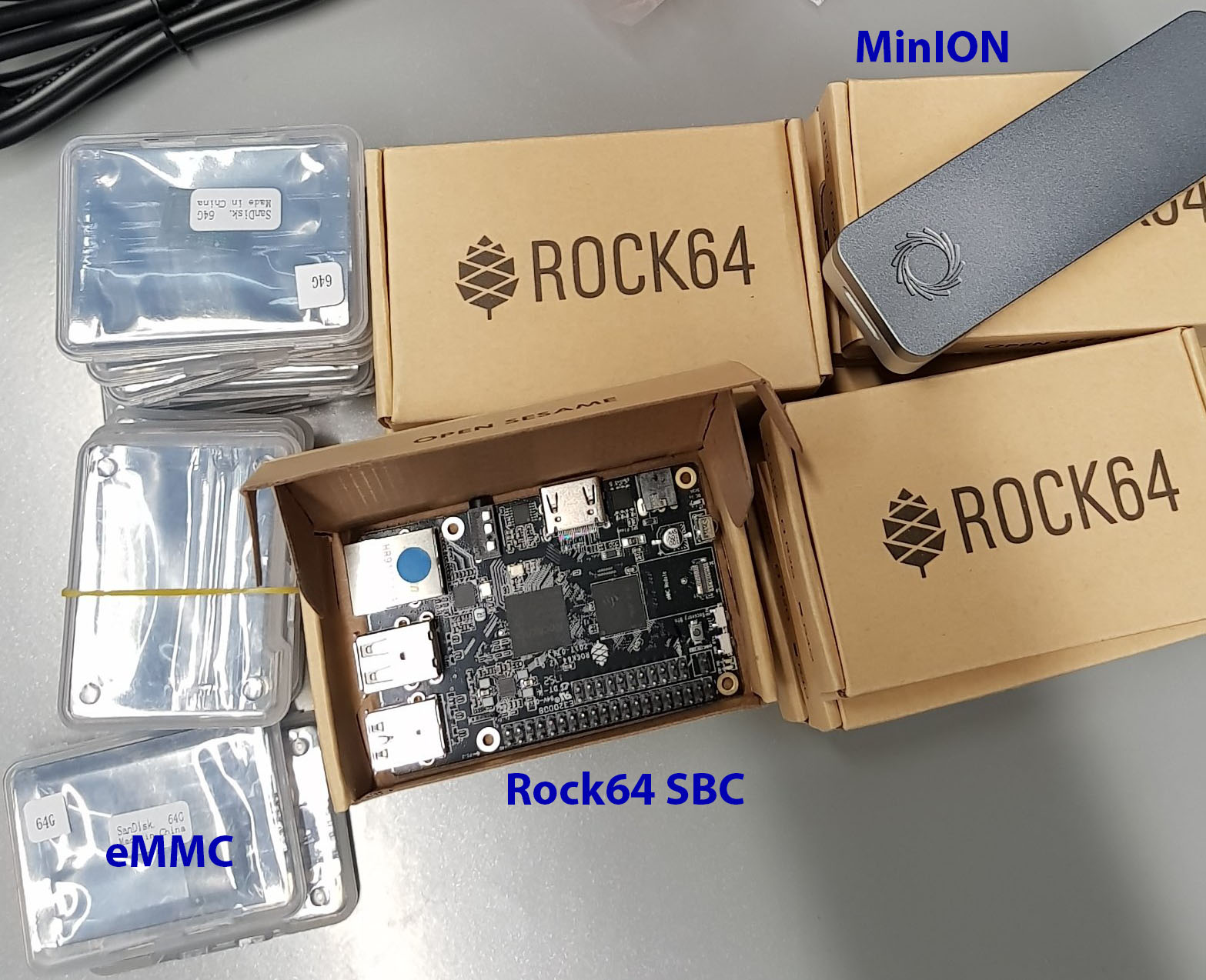
(a) A newly opened Rock64 SBC. Photograph credit: Martin A. Smith.

(b) Rock64 SBCs stacked using M2.5 cylinders. Photograph credits: Martin A. Smith.

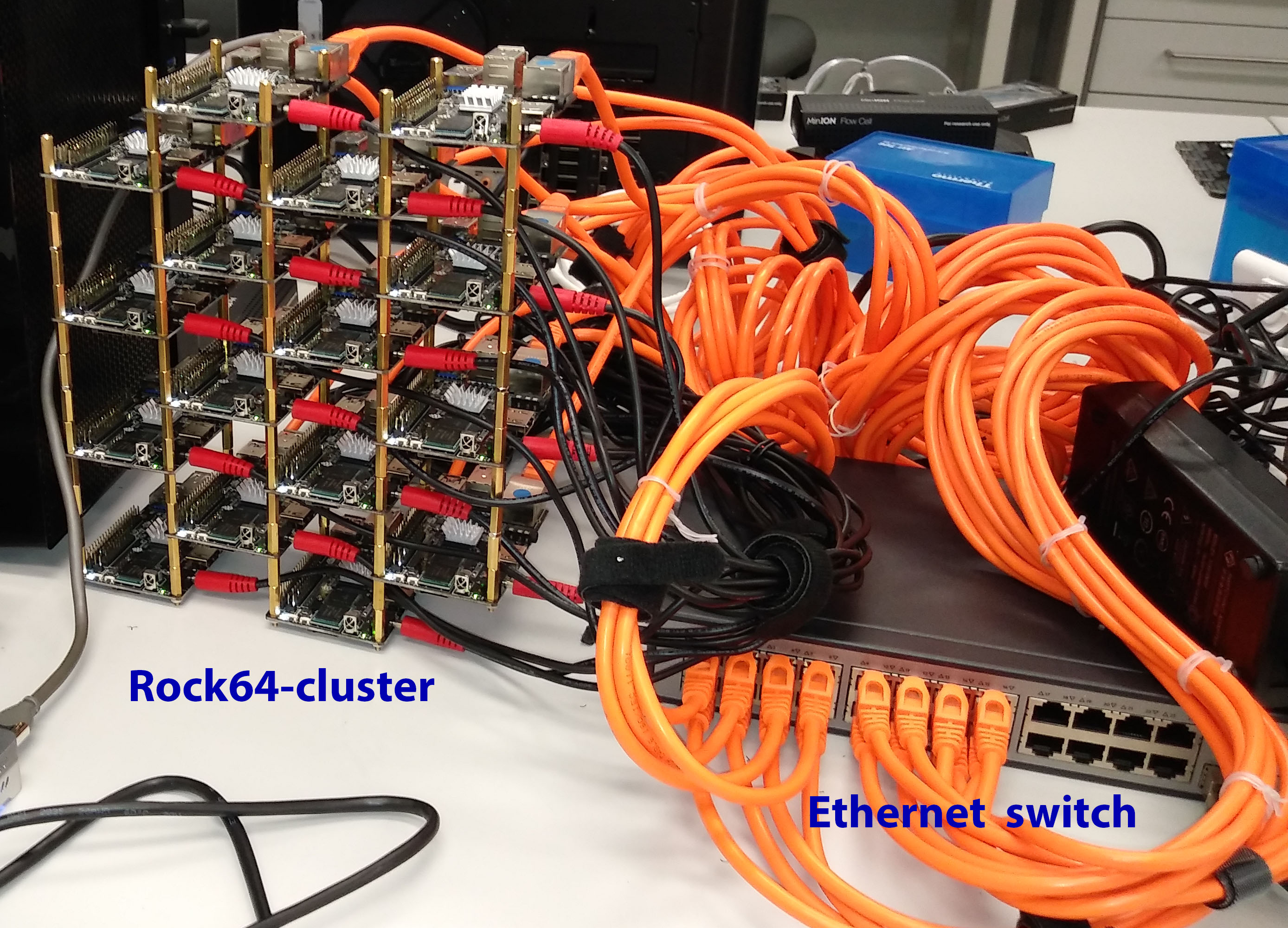
(c) Rock64 SBCs connected using Ethernet

Figure 6.3: Construction of the Rock64-cluster.

6.3.2 Rock64-cluster Software Setup

f5pd and f5pl proposed in section 6.2.2.3 were implemented in C programming language. TCP sockets were used for communication between f5pd and f5pl. Multiple worker nodes were handled in f5pl using multiple threads implemented with pthreads. f5pd was launched at the startup of each worker node and was ensured for continuous running using systemd. TCP keepalive feature in the Linux kernel [204] was used to detect hung worker nodes (by determining if the connection is still up and running or if it has broken).

The Rock-64 cluster was evaluated using a state-of-the-art nanopore methylation calling workflow (presented previously in Fig. 6.4) consisting of software tools Minimap2, Nanopolish and Samtools. The optimised version of Minimap2 for efficient memory capacity under chapter 4 is used on the Rock64-cluster where the original Minimap2 cannot run due to limited RAM on each node. Samtools was compiled for ARM architecture. A modified version of Nanopolish was initially used on the Rock-64 cluster, which was eventually replaced with f5c developed in chapter 5. Original Nanopolish which did not compile on ARM due to Intel specific SSE instructions had to be modified and a bug that affected ARM architecture had to be fixed to successfully run on ARM architecture. These fixes are now on the original Nanopolish repository, see appendix G. Later Nanopolish was replaced with f5c as f5c for faster performance and memory efficiency. Despite, Rock64 devices not having a GPU, f5c was around twice faster compared to Nanopolish.

The aforementioned workflow was implemented as a shell script. This pipeline shell script runs on each worker node for each data as mentioned in section 6.2.2.3. The shell script first copies data from NAS to local eMMC storage and (extract if a single-fast5 tarball), performs the commands of the aforementioned pipeline in the order presented in Fig. 6.4 and finally copies the result back to the NAS.

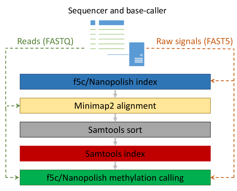
Figure 6.4: Methylation calling workflow and its software tools

Ansible was used to automate administration task such as deploying software updates across worker node, configuring settings across all worker nodes, performing maintenance operations etc. Ansible installed on the head node accesses worker nodes through password-less key-based SSH. the ganglia monitoring system [205] was set up on the nodes to centrally observe the state and the utilisation of worker nodes from the head node (screenshot in Fig. 6.5). Also, rsyslog coupled with loganalyzer [206] was configured to centrally view the worker node logs from the head node (screenshot in Fig. 6.6).

The detailed steps to install and manage the Rock64-cluster are in E and the associated scripts are in the GitHub repository at https://github.com/hasindu2008/nanopore-cluster. Source code of f5p is available at the GitHub repository https://github.com/hasindu2008/f5p and more details are in appendix E.2.

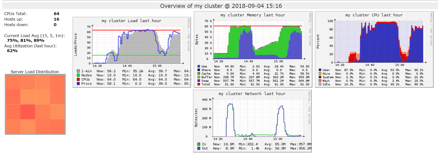
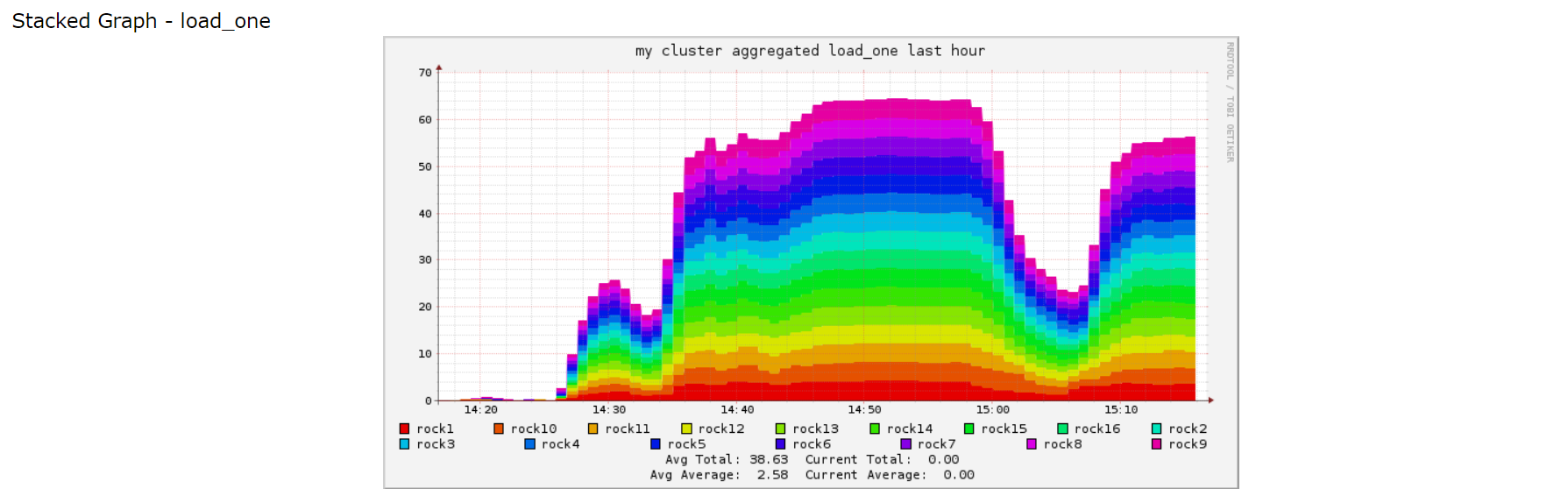
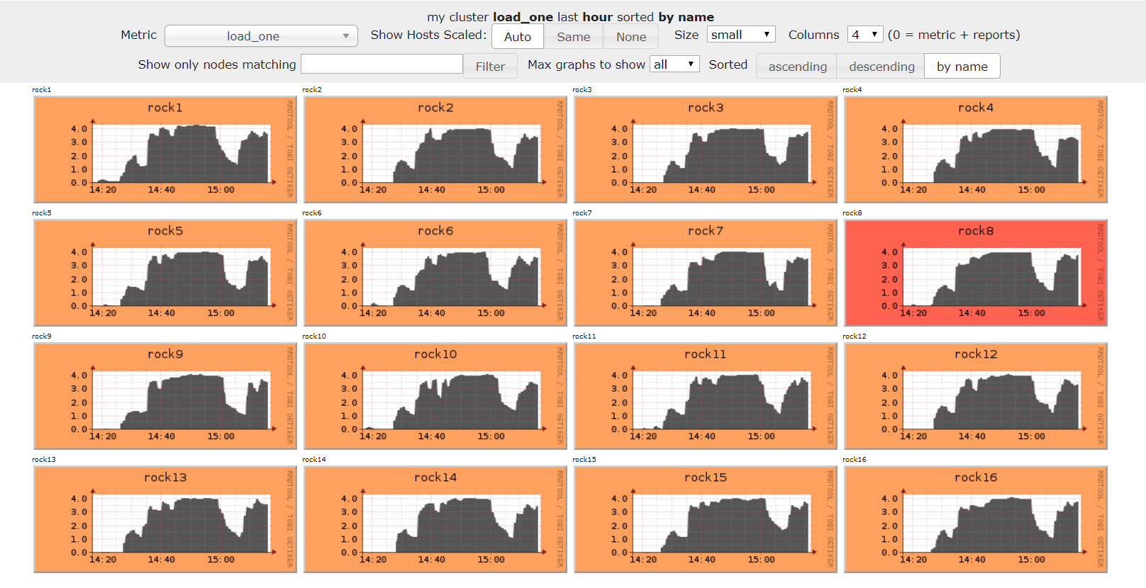
Figure 6.5: Screenshot from Ganglia monitoring system

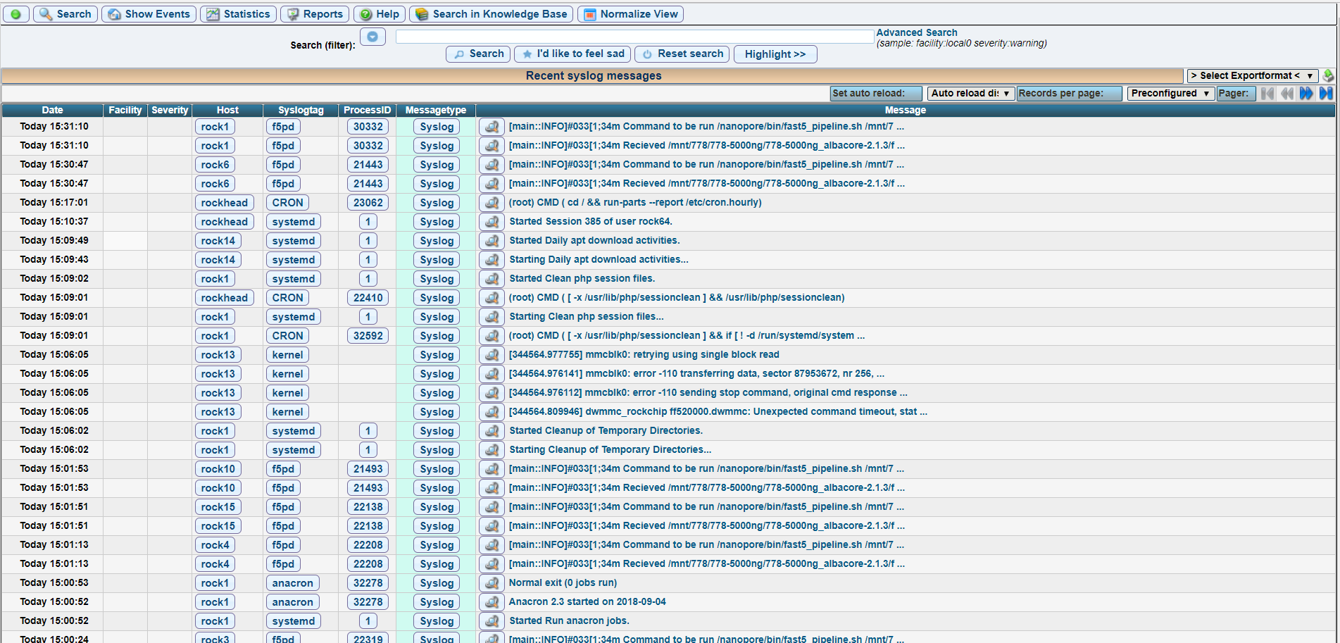
Figure 6.6: Screenshot from LogAnalyzer

6.3.3 NVIDIA Jetson SBCs

The architecture presented in section 6.2.1 is not limited to Rock64 devices, instead can be any other SBC. Two other SBCs, namely Jetson TX and Jetson Nano from NVIDIA, were evaluated as an alternative to Rock64. However, due to prohibitive cost of building a complete cluster of the Jetson SBCs, this evaluation was performed only using a single worker node, which is adequate as the multi-node architecture was already verified using Rock64 SBCs.

Jetson TX2 development board (Fig. 6.7(a)) is composed of a hexa-core ARM processor, 256 GPU cores, 8GB of memory (shared RAM for CPU and GPU) and 32 GB eMMC integrated storage. A Samsung 1TB SSD drive was connected to the Jetson TX2 development board using the SATA interface. The system was running on Ubuntu 16.04.

Jetson Nano development (Fig. 6.7(b)) is composed of a quad-core ARM processor, 128 GPU cores and 4GB of memory (shared RAM for CPU and GPU). A Sandisk Extreme 64GB microSD (A2 rating) and a Samsung 512 GB external SSD USB drive were used as the storage. This system was running on Ubuntu 18.04.

The evaluation was performed using the same methylation workflow used for the Rock64-cluster in section 6.3.2, with the use of f5c CPU-GPU version instead of the CPU-only version being the only difference.

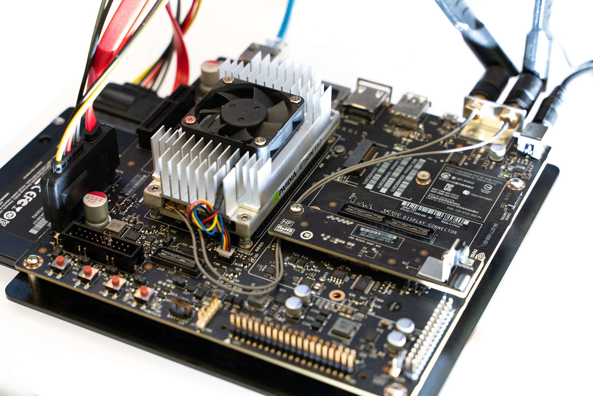
(a) Jetson TX2 development board

(b) Jetson nano development board

Figure 6.7: NVIDIA Jetson development boards. Photograph credits: Hsu-Kang Dow.

6.3.4 Datasets

A Nanopore MinION dataset of the T778 cancer cell-line of the human genome was used for the evaluations presented in section 6.4. This dataset contained 771,325 reads with 11,393 and 194,983 as the average and maximum of read lengths. The total yield was 8.78 Gbases and total sizes of FAST5 and FASTQ files were 845GB and 17GB respectively. The FAST5 files were of the single-FAST5 format. The dataset consisted of 198 batches of reads with each batch having 4000 reads.

6.4 Results

6.4.1 Rock64-cluster

For the aforementioned T778 MinION dataset, the complete methylation calling workflow consumed 5.88 hours on the Rock64-cluster. These 5.88 hours include the total processing time (processing steps in Fig. 6.4) and all the overheads, i.e., overheads due to scheduling, file transfer to/from the NAS and tarball extraction. The tool used for methylation calling was f5c. Note that, the time for the complete analysis on the Rock64-cluster (5.88 hours) is considerably lesser than the sequencing runtime on the MinION (typically 48 hours).

During the analysis time (5.88 hours) mentioned above, five occasions of worker node freezes were recorded (worker node freezes explained in section 6.2.2.3). Four of the freezes resulted in watchdog time outs and eventually automatic restarts. However, the integrity of the analysis was not affected due to the failure handling mechanism of f5p that reassigned the data batch once the worker node became alive (detailed in section 6.2.2.3). One freeze led to a totally dead device (not restarted by the watchdog), however, the analysis was continued with the remaining devices by f5p as mentioned in section 6.2.2.3. Note that, the 5.88-hour analysis time includes the time lost due to these freezes and dead devices.

The summary of execution details discussed above for the T778 MinION dataset is listed in the first row of Table 6.1. In Table 6.1, the first column describes the sample that is sequenced, the second column indicates the nanopore sequencer used (whether MinION, GrdION or PromethION), the third column lists the number of data batches in the dataset, the fourth column gives the typical sequencing runtime (48h for MinION/GridION and 64h for PromethION), the fifth column indicates the software used for methylation calling (f5c or nanopolish), the sixth column gives the total time for the execution of the methylation calling workflow on the Rock64-cluster, the seventh column gives the number of worker node freezes that were detected by the watchdog timer leading to automatic restarts and the eighth column gives the number of worker nodes retired due to complete freezes or consecutive failures.

While the above T778 dataset was used for performing thorough evaluation and benchmarks, several other nanopore datasets were processed on the Rock64-cluster and their execution details are summarised in Table 6.1 from the second row onwards. These details were collected while using the Rock64-cluster for in-house data processing of research data samples. Some datasets in Table 6.1 have been processed using Nanopolish instead of f5c because those were processed before the development of f5c as mentioned in section 6.3. The last two rows of Table 6.1 are for the same dataset where one execution was using f5c and the other using nanopolish. Observe that f5c performance is superior (45.08 hours for the complete workflow) compared to Nanopolish (61.58 hours for the complete workflow), in spite of 3 worker nodes being retired in the f5c execution compared to only 2 retired worker nodes in the Nanopolish execution. Therefore, the processing time observed for the datasets processed using nanopolish would be improved if executed using f5c.

Table 6.1: Execution results of several nanopore datasets of the human genome on the Rock64-cluster

Sample	Sequencer	Data batches	Sequencing run time (h)	f5c or Nanopolish	Processing time (h)	Node resets	Node retires
T778 - lipsarcoma	MinION	198	48	f5c	5.88	4	1
MCF7 - breast cancer	GridION	727	48	Nanopolish	18.08	1	0
MCF7 - breast cancer	GridION	447	48	Nanopolish	11.47	1	1
NA12878	PromethION	2954	64	f5c	50.27	5	1
HCT116A - colon cancer	PromethION	1613	64	Nanopolish	47.58	5	1
Dk01 - prostate cancer	PromethION	2659	64	Nanopolish	85.28	5	2
LNCap - prostate cancer	PromethION	2858	64	Nanopolish	65.70	1	2
PrEC - Prostate Epithelial	PromethION	1256	64	Nanopolish	45.52	5	0
T778 - lipsarcoma	PromethION	1210	64	Nanopolish	35.63	1	0
HBB20 PBMC	PromethION	2145	64	f5c	45.08	3	3
HBB20 PBMC	PromethION	2145	64	Nanopolish	61.58	4	2

6.4.2 On NVIDIA Jetson SBCs

The architecture proposed in section 6.2 is generic, i.e., worker nodes are not limited to Rock64 SBCs. Two alternative SBCs to Rock64 were benchmarked, namely, Jetson TX2 and Jetson Nano. Both Jetson SBCs are from NVIDIA and are equipped with GPUs making it possible to fully harness the GPU accelerated component of f5c. The benchmarking was performed only on a single Jetson TX2 and a single Jetson Nano due to prohibitive costs. The performance of the methylation calling workflow on each of these SBcs is compared to the performance on a single Rock64 SBC in Fig. 6.8.

The x-axis of the horizontal bar chart in Fig. 6.8 denotes the time in hours. The bars denote the sum of execution times for all the 198 batches of the T778 MinION dataset and different colours denote the breakdown of the execution time for each step in the workflow. Jetson TX2 was the fastest, consuming 12.27 hours, followed by Jetson Nano consuming 31.44 hours. Rock64 was the slowest consuming 60.31 hours. Thus, a single Jetson TX2 was around 5 times faster when compared to a single Rock64 SBC and a single Jetson Nano was around 2 times faster than a single Rock64 SBC.

On each SBC, the major portion of the time was contributed by the Minimap2 alignment step (49%-60%) followed by the methylation calling step (33%-43%). Methylation calling was performed using f5c, the CPU-only version on Rock64 and the CPU-GPU version on the Jetson SBCs. f5c index contributed less than 7% of the total time and the times for Samtools sort and Samtools index were very small (around 1%).

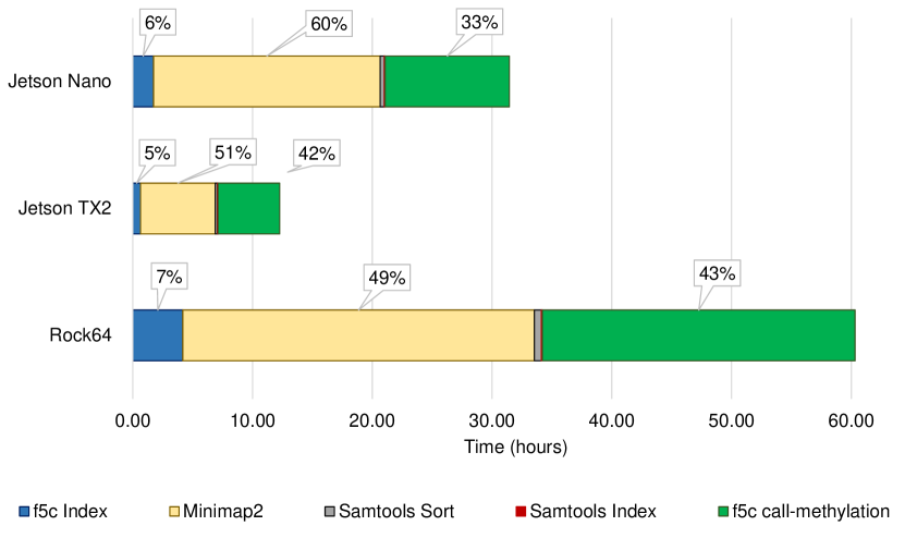
Figure 6.8: Comparison of Jetson TX2, Jetson Nano and Rock64 based on the single SBC execution times for the whole dataset

Fig. 6.9 shows the workflow execution time spent on each data batch of the 198 data batches of the T778 dataset. Fig. 6.9(a) is for a single Rock64, Fig. 6.9(b) is for a single Jetson TX2 and Fig. 6.9(c) is for a single Jetson Nano. The x-axis of each bar chart denotes the data batch number ranging from 1 to 198. The y-axis is the time in minutes where the bars represent the time spent on each data batch for the methylation calling workflow. Different colours in bars denote the breakdown of the time for different steps in the workflow. The average time for processing a data batch was 18.35 minutes for the Rock64 SBC, 3.72 minutes for the Jetson TX2 and 6.39 minutes for the Jetson Nano. Out of the 18.35 minutes for the Rock64, the major portion was consumed by Minimap2 alignment (8.95 minutes) followed by f5c methylation calling (7.90 minutes). Similarly, 1.89 and 1.56 minutes for Jetson TX2 and 5.73 and 3.14 minutes for Jetson Nano were recorded for Minimap2 and f5c, respectively.

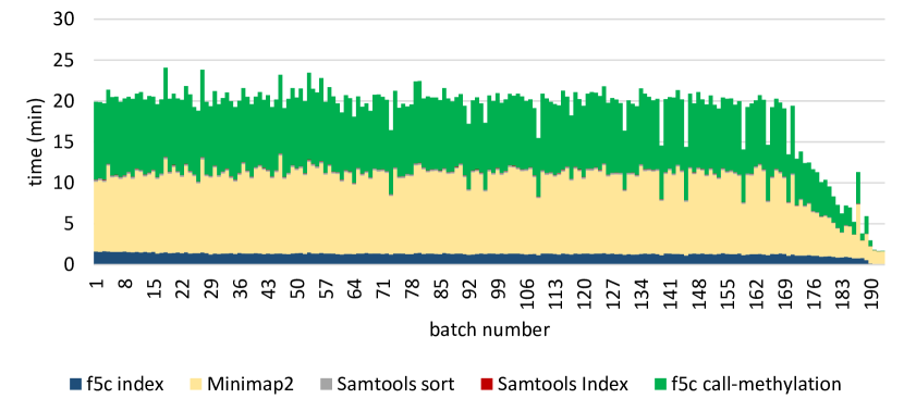
(a) On a single Rock64 development board

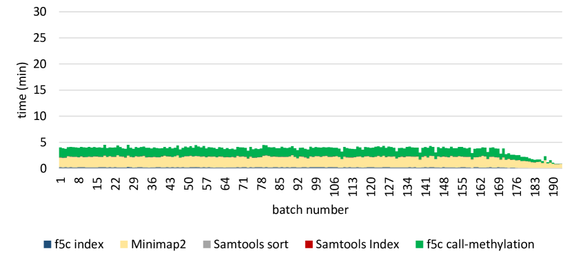
(b) On a single Jetson TX2 development board

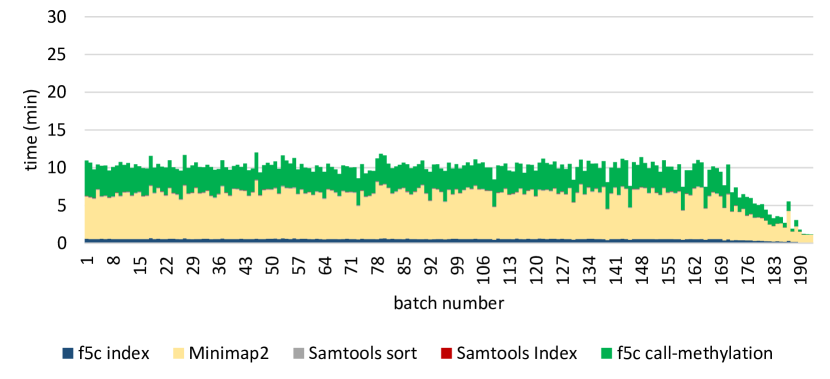
(c) On a single Jetson nano development board

Figure 6.9: Execution time on individual SBCs per each batch in the dataset

6.4.3 Real-time Processing Capability

As mentioned in section 6.1, nanopore sequencers are capable of streaming the sequencing data and thus it is possible to process data on-the-fly. This section demonstrates the proof of concept of performing data analysis on-the-fly (real-time) using the architecture presented in section 6.2.

How the sequencing rate varies over time is shown in Fig. 6.10 for MinION (blue curve), GridION (orange curve) and PromethION (yellow curve). The x-axis denotes the time in hours and the y-axis denotes the cumulative number of bases sequenced (in Gbases) over time. Observe how the sequencing rate (gradient of the curve) is high at the beginning, when then slowly reduces and eventually becomes zero.

Fig. 6.10 also plots the cumulative number of bases possible to be processed using a single Rock-64 SBC (purple dashed line), a single Jetson TX2 (blue dashed line) and a single Jetson Nano (green dashed line). For these plots, the y-axis is now the number of gigabases analysed. The gradient of each plot is calculated by dividing the total workflow execution time in Fig. 6.8 for the corresponding SBC by the total number of bases in the dataset. Observe that a single Rock64 device is barely adequate to keep up with the MinION curve. At first, the analysis lags when the sequencing rate is high, which then catches up when the sequencing rate drops. Observe that, a single Jetson Nano can easily keep up with a MinION and a Jetson TX2 is barely adequate to keep up with the GridION curve. Fig. 6.10 also plots the cumulative number of bases possible to be processed using clusters made of each SBC., i.e., 16 Rock64 devices (purple dotted line), 4 Jetson TX2s (green dotted line) and 8 Jetson Nanos (blue dotted line). The gradients of these lines are equal to the product of the gradient for a single SBC and the number of devices. The number of SBCs in a cluster has been selected so that the cluster can more than adequately keep up with a PromethION flowcell. Such an extra margin between the analysis and the sequencing yield curves will smooth on-the-fly processing while allowing for disruptions such as device freezes.

Note that the x-axis in Fig. 6.10 shows only the first 45 hours of the sequencing run as the curve is almost flat by this time, despite the sequence run of a MinION/GridION being 48 hours and PromethION being 64 hours. Also, the curves for the sequencers in Fig. 6.10 are based on typical average values. The exact curve can vary based on factors such as the quality of the sample and flow cell and also will change with technology improvements. Nevertheless, the presented proof of concept technique for estimating the number of SBCs for analysing data on-the-fly remains unaffected.

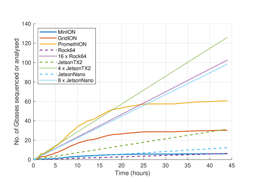
Figure 6.10: The comparison of the sequencing rate with the data analysis rate over the duration of the sequencing run

6.4.4 Comparison with HPC

The performance of the Rock64-cluster is compared to the performance of an HPC in Fig. 6.11. The Rock64-cluster performed the methylation calling pipeline using f5p as explained in section 6.3. The HPC was a server with 28 Xeon E5-2680 cores, 512GB RAM and 10 NVMe SSD drives in RAID configuration. The HPC executed the same methylation calling workflow as in Fig. 6.4 with original Minimap2 and original Nanopolish. Observe that the time spent on the Rock64-cluster (5.88 hours) is comparable to the time consumed on HPC (4.81 hours). Importantly, the time for Rock64-cluster includes the overheads for copying to/from the NAS and extracting tarballs whereas the HPC processed the dataset that was already placed on the fast local SSD RAID drives.

Comparing the cost and size of the Rock64-cluster with that of the server (about 10 times approximately), it is surprising that the performance is similar. Further analysis of this surprising phenomenon is in chapter 7.

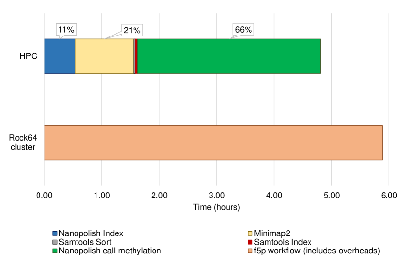
Figure 6.11: Comparison of proposed architecture on the Rock64-cluster with the original pipeline running on an HPC

6.5 Discussion

6.5.1 Implementation for On-the-fly Processing

The evaluation results presented on this chapter were based on datasets that were already residing on the NAS (datasets of previously sequenced samples), i.e., the whole dataset (all data batches) was available on the NAS when the workflow execution was started on the Rock64-cluster. While being adequate to demonstrate the proof of concept for on-the-fly (real-time) data processing, the future work could focus on implementing the scripts that automates the data transfer in real-time from the sequencer to the NAS. In fact, this implementation work is currently under progress as an undergraduate student project (https://github.com/sashajenner/realf5p) and is not claimed as a part of this thesis.

6.5.2 Mobile Phone Cluster

The proposed architecture in this chapter can also applicable to a cluster of mobile phones connected through Wi-Fi. The feasibility of performing the methylation calling workflow on an Android mobile phone was evaluated in an experimental environment (Fig. 6.12) as described in Appendix F. The development of a proper Android Application was undertaken by an undergraduate project group and is described in the pre-print at [28]. Also, the Wi-Fi cluster implementation is under progress by the same group. The development of the Android application or the Wi-Fi cluster is not claimed under the thesis.

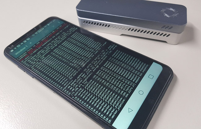
Figure 6.12: Methylation calling workflow on an Android mobile phone

6.5.3 Potential Diagnostic Applications

The proposed architecture that realises portable real-time nanopore-based methylation detection systems has potential applications such as tissue classification, diagnostic tests, environment, age, etc. The basis for such an application is in Fig. 6.13 that shows how the methylation frequency changes with the number of bases sequenced for five different loci on the human genome (TP53, MGMT, BRCA1 and BRCA2 that are genes and chromosome 22). The number of bases sequenced (x-axis) is indicative of the time. As observed in the left plot in Fig. 6.13, most of the CpG sites in the genomic locus are covered after around 2 gigabases of sequencing data (the gradient of the curves decreases). The right plot in Fig. 6.13 shows that the methylation frequency across various loci stabilises after around 2 Gbases of sequencing data.

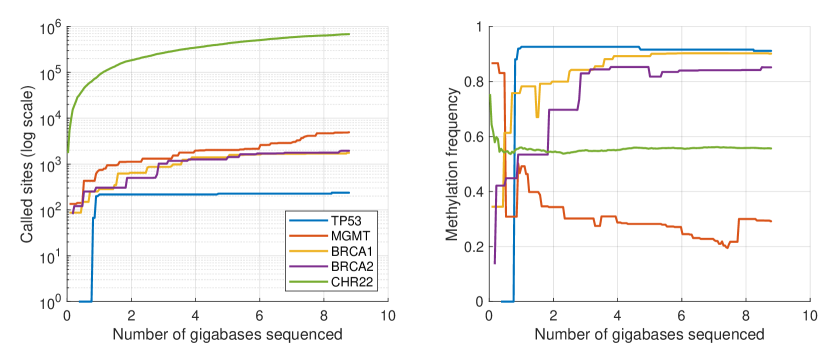
Figure 6.13: Potential applications of real-time methylation calling. Left graph - the variation of the number of called sites and the methylation frequency over the number of gigabases sequenced

6.6 Summary

A system architecture was proposed for performing a popular DNA methylation detection workflow on a prototype embedded system. The workflow was realised on the proposed architecture by integrating the optimised software versions from previous chapters. The proposed architecture was evaluated using off-the-shelf single-board computers and was demonstrated that performing real-time analysis of nanopore sequencing is possible on an embedded system. Also, it was shown that the performance of the prototype embedded system is surprisingly similar to the performance on an HPC. The prototype system is fully functional and is integrated into the nanopore sequencing facility at the Garvan Institute of Medical research for performing methylation calling of the samples. The system architecture and the associated software for building a replica of the prototype are open-sourced at https://github.com/hasindu2008/nanopore-cluster and https://github.com/hasindu2008/f5p.

Chapter 7 Optimisation of Nanopore Sequence Analysis for Many-core CPUs

  This chapter is prepared to be submitted as a publication in an ACM/IEEE journal/conference: H. Gamaarachchi, H. Saadat, S. Parameswaran, "Optimisation of Nanopore Sequence Analysis Software for Many-core CPUs", to be submitted [in progress], 2020.
 

Nanopore sequencing is a third generation (the latest) genome sequencing technology. These modern advances in computational genomics are reshaping healthcare through life-saving applications in medicine and epidemiology, where quick turn-around time of results is critical. Nanopore sequence analysis software tools are inefficient in utilising the computing power offered by modern High Performance Computing systems equipped with many-core CPUs and RAID systems. In this chapter, we present a systematic experimental analysis to identify the potential bottlenecks, which reveals that the primary bottleneck is the thread-inefficient HDF5 library used to load nanopore data. We propose multiple optimisation strategies suitable for different practical scenarios to alleviate the bottleneck: 1) a new file format that offers up to ${\sim}42\times$ I/O performance improvement; and, 2) a multi-process based solution for the scenario when using a new file format is not possible, that offers up to ${\sim}32\times$ I/O performance improvement.

We demonstrate the efficacy of our optimisations by integrating them to the popular Nanopolish toolkit. Our experiments using a representative nanopore dataset demonstrate that the proposed optimisations enable improved scaling of overall-performance with the number of threads (${\sim}6.5\times$ for 4 vs. 32 threads). Moreover, they also lead to overall-performance improvement (${\sim}2\times$ for 4 threads and ${\sim}6.5\times$ for 32 threads) and improved CPU utilisation (from 69% to 99% for 4 cores and from 22% to 85% for 32 threads) for a given number of threads, when compared to the original Nanopolish.

7.1 Introduction

Computational genomics has turned a new chapter in medical sciences and epidemiology [207, 208]. It enables promising applications such as accurate disease diagnosis, identifying genetic predisposition, and precision medicine [209]. Genome sequencing converts the genetic and biological information encoded in DNA molecules into computer readable data, which is typically hundreds or thousands of gigabytes in size. Nanopore sequencing is a leading third-generation (the latest) genome sequencing technology [189]. Computational genomics software tools analyse the huge amount of data generated by genome sequencing to extract meaningful information for the above applications.

Quick turn-around time of results in such applications is highly desirable. For instance, quick diagnostics can instantiate immediate treatments. Moreover, rapid results would enable faster tracking of disease spreading in epidemiological applications such as the ongoing Corona virus outbreak [210]. However, to analyse the enormous amount of data with high speed, genomic computation software tools demand massive computing time. Thus, scientists typically use High Performance Computing (HPC) systems to run these software tools [211].

A modern HPC system offers significant computational power through many-core CPUs that are to be exploited through parallelism. The major advantage in such systems when compared to an ordinary personal computer is the availability of number of cores in the CPUs. Moreover, HPC systems have RAID storage composed of many disks for higher I/O throughput with the added benefit of reliability [212]. Unfortunately, the existing software tools for nanopore sequencing are generally not capable of efficiently utilising the large number of cores available in many-core HPC systems, and thus fail to take maximal advantage of the available computing power. Consequently, the overall execution time of the applications on an expensive HPC system may not improve significantly when compared to its execution on a less expensive workstation or a personal computer (refer to chapter 6). In this chapter, we present software optimisations in nanopore software tools to enable them to take maximal advantage of the computing power offered by modern many-core HPC systems.

To demonstrate the problem mentioned above, we present a motivational example using Nanopolish [104], which is a popular state-of-the-art nanopore raw data analysis toolkit [213].

Motivational Example: We executed the call-methylation tool in Nanopolish toolkit on a representative dataset. The experiment was performed on a high-end HPC system with 36 Intel Xeon cores using different number of threads. The graph in Fig. 7.1a plots the execution time (y-axis) for Nanopolish against the number of threads (x-axis). We observe that when the tool is executed with four threads, the execution-time is nearly 10 hours. The execution-time does not improve significantly with increasing number of threads, and there is little improvement beyond 16 threads.

To analyse further, Fig. 7.1b plots the CPU utilisation (left y-axis) and the core-hours (right y-axis) for each case in the above experiment. The CPU utilisation, for execution with four threads, is less than ideal (69%). Moreover, as the number of threads increase, the CPU utilisation decreases significantly. Specifically, when executed with 32 threads, the CPU utilisation is as low as 22%. We also observe that the core-hours (which should be constant with the number of threads in an ideal case) increase significantly, and hence depicting that employing greater number of threads is inefficient and not highly beneficial.

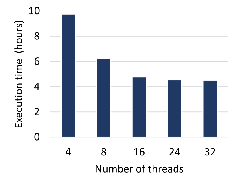
(a) Execution time

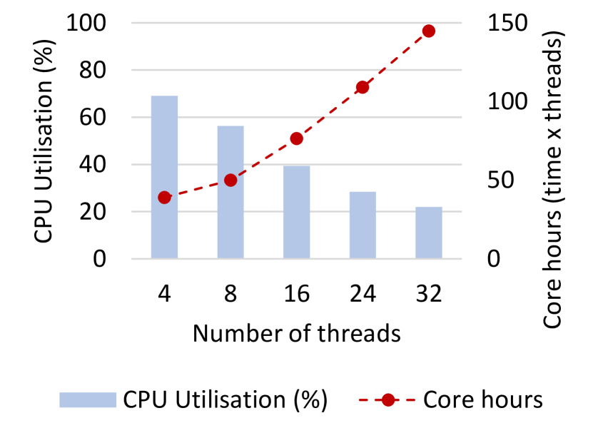
(b) CPU utilisation & core-hours

Figure 7.1: Variation of (a) execution time, (b) CPU utilisation and core-hours in original Nanopolish with the number of data processing threads.

Thus, procuring an HPC system with a higher number of CPU cores might not be beneficial for achieving quick turn-around time of results for nanopore software tools, and there is a need for software optimisations in nanopore software tools to exploit the available resources in HPC systems. To this end, in this chapter, we first present a systematic experimental analysis to identify the potential bottlenecks that hinder the efficient utilisation of CPU resources in nanopore software tools. Then we present multiple optimisations–suitable for different practical scenarios–to overcome these bottlenecks and enable performance improvements. Our experiments using the state-of-the-art Nanopolish toolkit on HPC systems demonstrate that our proposed optimisations enable improved CPU utilisation and hence improved performance scaling with the number of threads (Fig. 7.9 and 7.11). Moreover, they also enable improved performance for a given number of threads with respect to the original Nanopolish. For example, for 32 threads, the CPU utilisation increases up to ${\sim}$85% (which was 22%), and a ${\sim}6.5\times$ speed up is achieved when compared to the original Nanopolish. We believe that such improved performance will facilitate fast diagnostics and rapid epidemic response.

Contributions: The key novel contributions of this chapter can be summarised as follows.

• We, for the first time, present a systematic analysis to identify the potential bottlenecks in nanopore software tools. The analysis reveals that the primary bottleneck is caused by a limitation in an underlying library (HDF5) that serialises disk accesses from multiple threads (Section 7.3).

• We propose an alternate file format (SLOW5) that alleviates the bottleneck by allowing random accesses from multiple parallel threads. The proposed file format is designed by exploiting the domain knowledge of nanopore sequencing (Section 7.4.1).

• In some scenarios, it may not be practically possible to use a new file format. Therefore, we present a second solution based on multi-processes. This solution alleviates the bottleneck without requiring any modification to the existing file format (Section 7.4.2).

• We demonstrate that the new multi-FAST5 file format–which is projected as a replacement of the existing FAST5 file format by the research community–also suffers from the same bottleneck, thus our proposed SLOW5 format is superior. Moreover, our multi-process based solution is also effective in alleviating the bottleneck in multi-FAST5 (Section 7.5.5).

chapter Organisation: Section 7.2 discusses the background and related work. Section 7.3 elaborates our analysis for identifying bottlenecks and its explanation. Our proposed optimisations and solutions are presented in Section 7.4. Section 7.5 presents our experimental setup and results. Finally, Section 7.6 is the discussion and the chapter is concluded in Section 7.7.

7.2 Background

7.2.1 I/O

Two types of I/O: synchronous I/O (blocking I/O) and asynchronous I/O (non-blocking I/O) are in the context of random accesses (opposed to sequential/streaming access) are discussed in subsections 7.2.1.1 and 7.2.1.2, respectively.

7.2.1.1 Synchronous I/O

Synchronous I/O is convenient to be programmed, and such programmed code are legible. Thus synchronous I/O is the most popular and predominantly used amongst typical programmers. Following is a simplified account of how random disk requests are served in a modern operating system.

Consider a single-threaded program that requests I/O using standard read or write system calls (buffered read/write API calls such as fwrite, fread, fprintf, getline, etc are eventually mapped to these system calls). These system calls are synchronous calls which return when the requested data is read from the disk.

In Fig. 7.2, the user-space thread is performing a synchronous I/O request. The operating system receives the system call and queues the disk request in its disk request queue. Momentarily, the user-space thread is put to sleep by the operating system, since a disk request is expected to take hundreds of thousands of CPU clock cycles. The operating system will schedule the disk request (assign to the disk controller) based on policies and priority levels imposed. The disk controller will perform the operation and the operating system will wake up the thread, once requested data reading is completed. If the disk system has a single disk, effectively one request can be served at a time. If the disk system has $K$ disks, up to $K$ requests may be served simultaneously, depending on the RAID level; i.e. $K$ simultaneous parallel reads are possible on a RAID 0 system with $K$ disks.

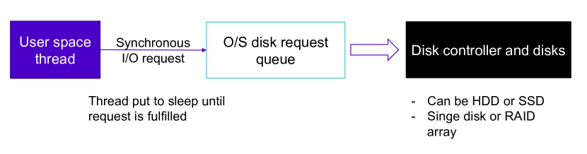
Figure 7.2: Elaboration of synchronous I/O

Consider a program with a single thread requesting I/O as shown in Fig. 7.2. Let $t$ be the average disk request service time (from the time of the system call to when the thread is woken up). Let a single thread be requesting $n$ synchronous disk reads sequentially. Despite the number of requests $n$, the total time spent on disk reading $T$ is : $T=t\times n$.

Now consider a program with multiple threads requesting I/O (I/O threads) as shown in Fig. 7.3. One thread put to sleep due to an I/O request, does not limit other threads from requesting I/O . Thus, if we launch $K$ I/O threads and if the disk controller can serve $K$ requests in parallel, the total time for disk reading is $T^{\prime}$ : $T^{\prime}=t\times\frac{n}{K}$

The scenario in Fig. 7.3 is achieved by programs where threads are having an independent code path - where each processing thread independently performs disk accesses on demand. However, in programs that perform data processing batch by batch, where one single thread reads a batch of data from the disk and assigns to multiple processing threads to be processed in parallel, it is the scenario in Fig. 7.2.

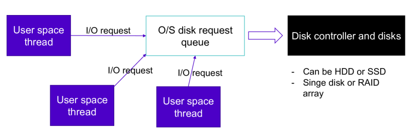
Figure 7.3: Elaboration of multi threaded synchronous I/O

7.2.1.2 Asynchronous I/O

Asynchronous I/O is pertinent to highly responsive applications like web servers and database servers. In asynchronous I/O, the system call that requests I/O will return immediately. The user-space thread won’t be put to sleep and this can continue to submit another I/O request or execute some other task while the disk request is being served.

Consider the asynchronous I/O example in Fig. 7.4 where a single thread submits multiple I/O requests to the operating system simultaneously. In Fig. 7.4, the single user space thread submits K I/O requests in parallel. Then the thread can either poll or wait for a notification from the operating system for I/O request completion. Assume we have $n$ total disk requests to be performed. If the disk system can perform $K$ accesses in parallel and if the time for a single disk accesses is $t$ ($K$ parallel accesses take $t$ as well), the total time $T^{\prime}=t\times\frac{n}{K}$. Note that the time is the same as for Fig. 7.3.

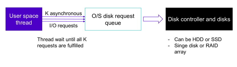
Figure 7.4: Elaboration of asynchronous I/O

This type of asynchronous I/O is suitable when a program performs reading data and processing batch by batch where one thread performs I/O and then assigns multiple threads or to an accelerator card (eg: GPU to be processed). This is in contrast to independently processing threads we discussed under synchronous I/O above, as threads need to converge in this case.

Asynchronous I/O can be performed by: (1) native synchronous I/O system calls in the operating system or (2) a library that emulates asynchronous I/O through a thread pool that use synchronous I/O system calls in the operating system.

From the two methods above, (1) allows ‘real’ asynchronous I/O, but only if supported by the operating system. Early Linux kernels (before version 2.5) did not have native asynchronous I/O systems calls, however, they are available in modern Linux kernels starting from version 2.5 onwards [215]. Despite that, asynchronous I/O implementation in the Linux kernel has been a controversial topic amongst Linux developers [216], is complicated [215], have various drawbacks [217, 215] and does not support certain file systems such as NFS [218]. GNU C Library (Glibc) does not provide wrapper functions for asynchronous I/O system calls [219]. Instead the programmers must use low-level system calls which are not easy and non-portable (Architecture specific). Third party libraries such as libaio [220] which uses Linux native asynchronous I/O system calls have attempted to provide an abstract interface.

An example of the method (2) above is the current Portable Operating System Interface (POSIX) compatible asynchronous I/O (AIO) library provided by Glibc. POSIX AIO implementation in GlibC is provided in the user-space and uses multiple threads [221]. The developer of POSIX AIO have admitted that their approach is expensive and have scalability issues which are expected to be fixed in the future through a state-machine-based implementation of asynchronous I/O [221]. Further, POSIX AIO is not implemented in all systems (eg: Windows subsystem for Linux)

While the POSIX AIO is suitable for typical I/O loads, the programmers can also spawn multiple I/O threads per batch and assign the disk accesses amongst them. This is suitable if the batch size is big and the thread spawning time is small compared to the I/O time of the batch.

7.2.2 Nanopore raw data analysis

Genomics: DNA is a molecule composed of a long strand of millions of units called nucleotide bases (or simply called bases). Genome sequencers read a DNA strand in relatively smaller fragments (around 10,000 bases long in nanopore) and converts them into digitised data, termed as reads[189] in the domain of bioinformatics. In this chapter we refer to them explicitly as genomic reads to avoid confusion with disk reads.

Nanopore Sequence Analysis: Nanopore sequencing is a leading third-generation (the latest) sequencing technology [189]. Oxford Nanopore Technologies (ONT) is the company that produces nanopore sequencers. A nanopore sequencer is composed of an array of pico-ampere range current sensors that measure the ionic current disruptions when DNA fragments pass through nanometer scale protein pores [189, 222]. The raw sensor output for a genomic read is a time series current signal and is referred to as raw signal or raw data. ONT stores the raw signal and other metadata (e.g., sampling frequency) in a file format called FAST5 [223]. FAST5 is essentially a Hierarchical Data Formats 5 (HDF5) [95] file with a specific schema defined by ONT. The only existing library for accessing HDF5 format is the official library developed and maintained by the non-profit organisation HDF Group [224, 225].

Nanopolish: Raw data analysis toolkits analyse the sequencer outputs using complex algorithms and extract meaningful information. Nanopolish is currently a popular state-of-the-art nanopore raw data analysis toolkit. Nanopolish is used in a number of genomic workflows such as methylation detection [104], variant detection [226], draft genome polishing [103, 56] and real-time molecular epidemiology for the ongoing Corona Virus outbreak [210]. Nanopolish is written in C/C++ and supports multi-threaded execution through OpenMP. It is an open-source toolkit with a large and complex codebase [104, 227].

Previous Work on Optimising Nanopolish: Nanopore sequence analysis is a relatively new field that only emerged in the last decade. Thus, optimisation efforts to improve performance of nanopore software tools are rare. In Nanopolish, calculation of log likelihood ratio is a predominantly used CPU intensive computation kernel [104]. To reduce CPU time for log likelihood computation, Nanopolish authors have already employed a fast table-driven log-sum implementation established elsewhere in [228]. However, none of the existing works have focused on improving the overall performance of Nanopolish on HPC systems with many-cores and Redundant Array of Independent Disks (RAID). Our proposed optimisations are orthogonal to the methods discussed above.

Previous Work on Optimising Sequence Analysis: Several optimisation efforts exist for the second generation sequencing software (also known as Next Generation Sequencing)  [229, 230, 231, 232, 24, 233]. However, software used for nanopore sequencing (third-generation) is distinct from the first and second generations [234]. Nanopore technology involves processing raw signal data, which is not the case for first and second generation.

In this chapter, we for this first time, identify the major causes behind the inefficient resource-utilisation by nanopore software tools and present multiple optimisations to alleviate those issues.

7.3 Identification and Explanation of bottleneck

The motivational example in Section 7.1 revealed that Nanopolish is unable to efficiently utilise multiple cores in the system. There can be two reasons for an application to be unable to utilise parallel resources. These are: 1) data processing bottleneck; and/or 2) I/O bottleneck. In this section, we identify and explain that the primary reason of the under-utilisation is I/O bottleneck.

7.3.1 Identification of the Bottleneck

We employed performance monitoring and profiling tools in the motivational example setup, to hypothesise the causes of inefficient resource-utilisation and performance.

Hypothesis-1: The performance of the software tool is bounded by file I/O. We observed through htop utility in Linux that majority of Nanopolish threads are in the ‘D’ state. The ‘D’ state is defined as the ‘state of the process for disk sleep (uninterruptible)’ [235]. This leads to our first hypothesis that the software tool is bounded by file I/O. In fact, Nanopolish incurs a large number of random disk accesses when reading millions of FAST5 files (based on HDF5) in a nanopore dataset.

Hypothesis-2: The file I/O bottleneck is caused by the HDF5 library and not by the limitation of physical disks. We observed the disk usage statistics through the iostat utility to find that disk system is not fully utilised (i.e., the observed number of disk reads per second was around 100, while the particular disk system could handle more than 1000 IOPS). This implies that I/O bottleneck is not due to the limitation of physical disks to serve data fast enough to saturate the processor. To investigate further, we profiled Nanopolish with Intel Vtune under concurrency profiling. It reveals that the majority of the ‘wait time’ is due to a conditional variable (synchronisation primitive) in the underlying library called HDF5 library (Hierarchical Data Format 5–used to access raw nanopore data stored in FAST5 file). A closer look into the HDF5 library revealed that the thread-safe version of the HDF5 library serialises the calls for disk read requests [236]. Thus, we hypothesise that the reduced CPU utilisation is caused by the disk requests being serialised by the HDF5 library, consequently causing the bottleneck and limiting the utility of a multi-disk RAID system.

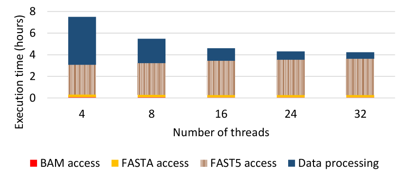
Figure 7.5: Decomposition of time for individual components in restructured Nanopolish.

7.3.2 Verification of the Identified Bottleneck

To verify the above identified cause of the bottleneck, we performed a deeper analysis. For this, we first restructured Nanopolish such that wall-clock time spent on I/O operations and data processing can be separately measured to determine the time spent on individual components in the program.

We run the restructured Nanopolish with various number of threads (for FAST5 access and data processing). The results are presented in Fig. 7.5. The x-axis in the figure represents the number of threads used and the y-axis represents the total execution time. Different colours in the bars (see legend) denotes the decomposition of the total execution time into different components.

We observe from Fig. 7.5 that: 1) the contribution by the BAM access and FASTA access to the overall execution time is negligible; 2) a major portion of the time is consumed by FAST5 access (patterned brown); 3) time consumption of FAST5 access (patterned brown) does not improve with increasing number of threads; and, 4) data processing time improves with increasing number of threads (solid blue). This confirms that the bottleneck is caused by file I/O and not because of any data processing bottlenecks.

7.3.3 Detailed Explanation of the Identified Bottleneck

In this subsection, we explain the major limitation in HDF5 library that prevents efficient parallel accesses, consequently causing the bottleneck.

HDF5 Library and its Limitations in Thread Efficiency: HDF5 library uses synchronous I/O calls and even the latest HDF5 implementation (HDF5-1.10) does not support asynchronous I/O. This, by itself, is not an issue as multiple synchronous I/O operations can be performed in parallel using multiple I/O threads to exploit the high throughput of RAID systems in HPC systems. Fig. 7.3 demonstrates how multiple I/O threads can be used to perform parallel disk accesses using synchronous I/O. Suppose the disk system has $K$ disks, up to $K$ requests may be served simultaneously depending on the RAID level; i.e., $K$ simultaneous parallel reads are possible on a RAID 0 system with $K$ disks. Let $t$ be the average disk request service time (from the time of the system call to when the thread is woken up). For a program that launches $K$ I/O threads and if the disk controller can serve $K$ requests in parallel, the total time for $n$ disk reads is $T^{\prime}=t\times\frac{n}{K}$.

However, the HDF group (that maintains the HDF5 library) mentions that the thread-safe version of the HDF5 library is not thread efficient and that it effectively serialises the calls for disk read requests [236]. The global lock in the thread safe version of the HDF5 library creates limitations. Following is an extract from the FAQ section of the HDF web site [236]. “Users are often surprised to learn that (1) concurrent access to different datasets in a single HDF5 file and (2) concurrent access to different HDF5 files both require a thread-safe version of the HDF5 library. Although each thread in these examples is accessing different data, the HDF5 library modifies global data structures that are independent of a particular HDF5 dataset or HDF5 file. HDF5 relies on a semaphore around the library API calls in the thread-safe version of the library to protect the data structure from corruption by simultaneous manipulation from different threads. Examples of HDF5 library global data structures that must be protected are the freespace manager and open file lists.”

Thus, in spite of having multiple I/O threads, I/O requests for HDF5 files have to go through the HDF5 library. Fig. 7.6 demonstrates this, where $K$ I/O threads are requesting I/O from the HDF5 library in parallel. However, the lock inside the HDF5 serialises the parallel requests, effectively issuing only one request at a time to the operating system disk request queue. The operating system will put the thread to sleep and this is equivalent to a single I/O thread. Thus, the total time spent on disk accesses $T$ will be $T=t\times n$, and essentially, the high throughput capability of multiple disks in a RAID configuration is under-utilised.

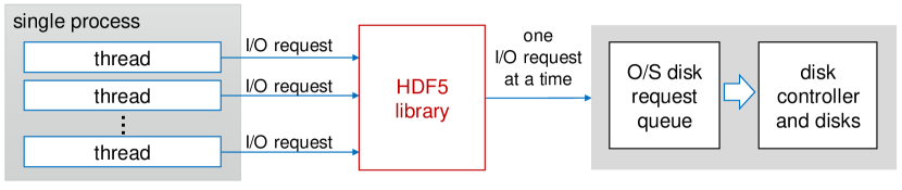
Figure 7.6: Elaboration of the limitation in HDF library.

7.4 Proposed Optimisations

In this section, we present two types of solutions to overcome the bottleneck in nanopore software tools. The first approach is to use an alternate file format (Section 7.4.1). However, current nanopore software tools have been developed on top of the FAST5 (HDF5) format because of its adoption by Oxford Nanopore technologies as the file format for storing the raw signal. Thus, using a new file format may not always be practical. For such scenarios, we present a second solution that uses multi-processes instead of multi-threads for I/O operations (Section 7.4.2). This second solution does not require any changes to FAST5 format or the HDF5 library. Furthermore, we also present a few more optimisations to Nanopolish that enable further speed-up (Section 7.4.3).

7.4.1 Alternate File Format (SLOW5)

We propose a new file format called SLOW5 for storing nanopore raw signal data as an alternate to FAST5. We considered the domain knowledge from nanopore sequence analysis and the characteristics of disk accesses to design the new file format.

SLOW5 File Format: We design our proposed SLOW5 file format by extending the simple and well-known tab-separated values (TSV) format, using inspiration from the gold standard genomic file formats such as SAM [57] and VCF [237]. An example of the proposed file format is shown in Table 7.1. The structure of the file is explained below.

The first set of lines of the SLOW5 file comprises the file header. Each header line starts with the character $\#$. Generic metadata such as the file version and global metadata of the sequenced genome sample are also stored in the header. The global metadata is common to all the genomic reads and contains information such as the sequencing flow-cell identifier, and sequencing run identifier, etc. The last line in the header gives the column names of the upcoming data, which are tab-separated. Note that, not all metadata and data fields are depicted in Table 7.1 for the sake of brevity.

The header is followed by data where each line (row) represents a single genomic read. In other words, for N genomic reads, there are N data lines in the file. The genomic read information fields (e.g., read-identifier, number of signal samples, and the raw signal) are tab separated and are in the same order as defined in the last line of the header. The raw_signal column contains the current signal values separated by commas. Note that all data corresponding to a single genomic read are placed contiguously in the same row, thus facilitating locality in disk accesses.

Working Explanation: Random accesses to the genomic read records in a SLOW5 file are facilitated by an index called the SLOW5 index. The SLOW5 index is another tab-separated file as shown in Table 7.2. Each line corresponds (except the first header line) to a genomic read. The first column is the read-identifier of the genomic read, the second column is the file offset to the corresponding SLOW5 record, and the third column is the size of the corresponding SLOW5 record in bytes (including the new line character). For performing random disk accesses to SLOW5, the SLOW5 index is first loaded to a hash table in RAM where the read-identifier serves as the hash table key and the rest of the data is used as hash table values. For a given read-identifier, the file offset and the record length is obtained from this hash table and the program can move the file pointer to the offset (i.e. using lseek) and load the record to the memory. Multiple random accesses to SLOW5 can be performed in parallel either through synchronous I/O calls with multiple threads, or through asynchronous I/O if supported by the operating system. Note that the raw signal data is read-only during nanopore sequence analysis. Thus, SLOW5 is inherently thread-safe without any need of global locks.

7.4.2 Multi-process based Solution

The original Nanopolish runs a single process with multiple threads. We propose a multi-process based solution for scenarios where the existing FAST5 cannot be replaced. Multiple threads in a single process share same address space and thus the lock in HDF5 library affects multiple threads. Multiple threads are typically used to run sub-tasks in parallel while conveniently sharing data amongst the threads. In contrast, multiple processes have their own independent address spaces and are typically used to run isolated tasks in parallel. We exploit the presence of independent address spaces in multiple processes to circumvent the lock in HDF5 library.

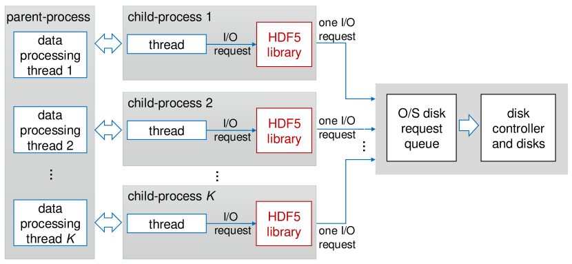
Figure 7.7: The proposed multi-process based solution.

Overview: Our proposed multi-process based solution is elaborated in  Fig. 7.7. We use multi-threads in the single parent-process for data processing and multiple child-processes for I/O. The parent-process performs data processing using multiple threads in parallel. Each child-process has its own instance of the HDF5 library, as a consequence of independent address spaces. Moreover, each child-process has only a single thread that requests I/O. Thus, a single instance of the HDF5 library gets only one request at a time. In effect, there are multiple instances of the HDF5 library that can submit multiple I/O requests in parallel to the operating system (as opposed to the situation in Fig. 7.6), thus benefiting from the high throughput offered by the RAID configuration. Formally, if there are $K$ processes and if the disk controller can serve $K$ requests in parallel, the total time spent on I/O operations will be $T^{\prime}=t\times\frac{n}{K}$ (similar to the case in Fig. 7.3).

Details: The proposed multi-process based solution can be adopted for Nanopore data processing using a pool of processes that performs FAST5 I/O. Multiple processes are spawned at the beginning of the program using the fork system call. These forked child-processes form a pool of processes that exist until the lifetime of the parent-process, solely performing I/O of FAST5 files. The data processing can be performed by multiple threads spawned by the parent-process as usual. The parent-process when it requires to load signal data of $N$ reads (FAST5 accesses), first splits the list of reads to $K$ parts where $K$ is the number of child-processes. Then, each part is assigned to each child-process, which performs the assigned FAST5 accesses. When data is loaded, the child-processes send data to the parent-process. The communication (data transfer) between the parent-process and child-processes can be implemented relatively easily using unnamed pipes out of the available Inter Process Communication (IPC) techniques (still not easy as threads that share the same memory space).

Note-1: A fork-join model for multi-processes (as could be done for the multi-threading) is unsuitable to be used instead of the process pool model presented above. Firstly, creating a process can be very expensive and could easily become the biggest bottleneck than the file reading itself. Secondly, forking in the middle of a program could double the memory usage and is usually problematic.

Note-2: We propose the use of multi-threads in the single parent-process for data processing and multiple child-processes for I/O. The possibility of using separate processes for both data processing and I/O is discussed in Section 7.6.1 with its caveats.

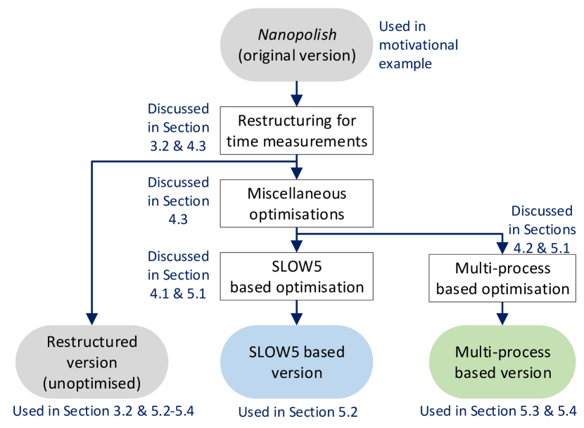
Figure 7.8: Flow diagram depicting modifications to Nanopolish

7.4.3 Restructuring & Miscellaneous Optimisations

In addition to the above I/O related optimisations, we also performed restructuring and a few other software optimisations with respect to multi-threading and memory. Our restructuring allows us to measure the execution time separately for I/O (including the execution time breakdown for different file formats) and data processing, without significant effect on performance, whereas, the software optimisation improve the processing time.

The original Nanopolish implementation uses openMP for multi-threading. We restructured Nanopolish to perform multi-threading using a lightweight fork-join model with work-stealing implemented using POSIX Threads (pthreads). Moreover, the restructured Nanopolish performs I/O operations and data processing batch by batch (batch of genomic reads), i.e., a batch of genomic reads are loaded from the disk and the batch is then processed, subsequently, results of the batch are written to disk. I/O operations are interleaved with data processing, i.e. when the first batch is being processed, the second batch will be loaded from the disk.

The restructured Nanopolish was further optimised with strategies such as: reducing the number of memory allocations (malloc) for dynamic 2D arrays by allocating a 1D array, an appropriate batch size that fits the available RAM, and a better load-balancing between multi-threads, etc. While space limits our ability to explain each of these optimisations, the details can be found in the open sourced code of this research project. For the sake of clarity, the overview of our restructuring and optimisations to original Nanopolish and various resulting versions with their usage, are shown in Fig. 7.8.

Table 7.1: Example of SLOW5 file format

SLOW5 file format
#fileformat: slow5v1.0
#exp_start_time: 2020-01-01T00:00:00Z
#run_id: 855cdb4b26948
#flow_cell_id: FAH00000
#read_id	n_samples	digitisation	offset	range	sampling_rate	raw_signal
read-0	123456	8192	6	1467.6	100000	498,492,501,508,503,505,509,…
read-1	2000	8192	5	1467.6	4000	400,401,500,403,407,478,510,…
.	.	.	.	.	.	.
.	.	.	.	.	.	.
.	.	.	.	.	.	.
read-N	10000	8192	3	1467.6	4000	559,545,560,551,550,565,701,…

Table 7.2: Example of SLOW5 index

SLOW5 index
#read_id	file_offset	rec_length
read-0	67	500000
read-1	500001	1000000
.	.	.
.	.	.
.	.	.
read-N	364459005610	1580072

7.5 Experiment and Results

7.5.1 Experimental Setup

Implementation of the Alternate File Format: We implemented a C program to convert FAST5 (HDF5) files into our SLOW5 format. The program also constructs a SLOW5 index as per the description in section 7.4.1. The restructured and optimised Nanopolish (discussed in section 7.4.3) was modified to support reading from SLOW5 format (Fig. 7.8). At the beginning of the program, the SLOW5 index is loaded onto a hash table that resides in RAM. For each genomic read in a batch, the start position of the corresponding SLOW5 record (file offset) and size of the record (in bytes) is obtained from the index. Then, that information for all the genomic reads in the batch are submitted as I/O requests. The POSIX AIO library in glibc is used for performing asynchronous I/O.

Implementation of the Multi-process Pool: The restructured and optimised Nanopolish was modified such that FAST5 files are loaded using a multi-process pool as per the description in Section 7.4.2 (Fig. 7.8). At the beginning of the program, $K$ child-processes are spawned using fork system call. Then, during the execution of the program, the parent-process divides the batch of genomic reads into $K$ parts and assigns each part to a child-process. Child-processes performs FAST5 file reading (through HDF5 library) in parallel. After completion of reading by the child-processes, the data is collected by the parent-process. The inter-process communication is implemented using unnamed pipes in Linux.

Datasets and Computer Systems:

A representative nanopore dataset of the human genome was used for the evaluation and the details are in Table 7.3. This dataset is a complete nanopore MinION dataset of the T778 cancer cell-line [238, 173]. The computer systems used for the experiments and their specification are given in Table 7.4. Unless otherwise stated, the experiments in the chapter have been performed on system S1. System S2 was used for limited number of experiments due to the limited availability. For the experiments associated with Network File System (NFS), the NFS storage on system S3 was mounted on system S1. For NFS, default parameters for the NFS server and client in Linux were used. Note that the operating system disk cache on S3 was also cleared before any NFS experiment.

Table 7.3: Dataset

ID	Sample	No. of Gbases	No. of reads	Average read length	Max read length	FAST5 file size
D1	T778	8.787	771 325	11 393	194 983	845GB

Measurements and Calculations: The measurement and calculations for our results are performed as follows.

1) The Overall execution time (wall-clock time) and the CPU time (user mode + kernel mode) of the program (all version shown in Fig. 7.8) were measured by running the program through GNU time utility in Linux.

2) The CPU utilisation percentage is computed as in equation 7.1. Note that this CPU utilisation percentage is a normalised value based on the number of data processing threads that which the program was executed with.

$$CPU\>utilisation=\frac{CPU\>time}{execution\>time\times number\>of\>threads}\times 100\%$$ (7.1)

Table 7.4: Computer systems

System ID	S1	S2	S3
Description	HPC with HDD RAID	HPC with SSD RAID	NFS server
CPU	2 $\times$ Intel Xeon Gold 6154	2 $\times$ Intel Xeon Gold 6148	4 $\times$ Intel Xeon X7560
CPU cores	36	40	32
RAM	384 GB	768 GB	256 GB
Disk System	12$\times$10TB HDD drives	6$\times$4TB NVMe drives	10$\times$3TB HDD drives
File System	ext4	ext4	ext4
RAID config.	RAID6	RAID0	RAID5
OS	Ubuntu 18.04.3 LTS	CentOS 7.6.1810	Ubuntu 14.04.6 LTS

3) Execution time for individual components (I/O operations and data processing) in the restructured and/or optimised Nanopolish (three versions at the bottom of Fig. 7.8) was measured by inserting gettimeofday function calls into appropriate locations in the software source code. To prevent the operating system disk cache affecting the accuracy of I/O results, we cleared the disk cache (pagecache, dentries and inodes) each time before a program execution. Despite the effect of the hardware disk controller cache (${\sim}$8GB) being negligible due to the large dataset size (${\sim}$850GB), we still executed a mock program run prior to each experiment. Note that the operating system disk cache on S3 was also cleared before any NFS experiment.

4) Core-hours is calculated as the product of the number of processing threads employed and the number of hours (wall-clock time) spent on the job. This metric is inspired by the metric man-hours used in labour industry and is used in Cloud Computing domain to calculate the data processing cost [214]. In an ideally parallel program, this metric remains constant with the number of cores/threads.

7.5.2 Results: Alternate File Format (SLOW5)

Overall Execution Time and CPU Utilisation: The overall execution time when our proposed SLOW5 file format is used in the restructured and optimised Nanopolish is shown in Fig. 7.9a, while the CPU utilisation and the core-hours are depicted in Fig. 7.9b. The x-axis represents the number of data processing threads which the program was executed with. The number of I/O threads for glibc POSIX AIO was also set to the same number of threads as the number of data processing threads.

Observation-1: Performance has improved w.r.t original Nanopolish for a given number of threads. To observe this, we compare Fig. 7.1a with Fig. 7.9a. At 4 threads, execution time improved by ${\sim}$2$\times$ compared to original Nanopolish. At 8, 16, and 24 threads speedups of ${\sim}$2.5$\times$, ${\sim}$4$\times$, ${\sim}$5.5$\times$ can be observed, respectively. At 32 threads, ${\sim}6.5\times$ speedup is observed. In other words, speedup of our optimised version over original Nanopolish increases with the number of threads.

Observation-2: CPU Utilisation has improved with the number of threads when compared with original Nanopolish. Comparing Fig. 7.1b with Fig. 7.9b reveals that CPU utilisation at 4 threads improved to 99% which was 69% for original Nanopolish. The CPU utilisation increases to 99% from 56%, 97% from 39%, and 92% from 28%, at 8, 16 and 24 threads, respectively w.r.t original Nanopolish. At 32 threads, an improvement of CPU utilisation to 85% was observed which was as low as 22% for original Nanopolish.

Observation-3: Performance scaling with number of threads is improved. This is evident by the core-hours plot in Fig. 7.9b, whose values are much smaller and almost constant when compared with its counter-part in Fig. 7.1b. For the original Nanopolish, the execution time with 32 threads improved only by ${\sim}$2.1$\times$ compared to running with 4 threads (from 9.7h to ${\sim}$4.5h). Our optimised version improved by ${\sim}$6.5$\times$ at 32 threads compared to 4 threads (${\sim}$4.5h to ${\sim}$0.7h).

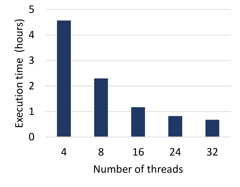
(a) Execution time

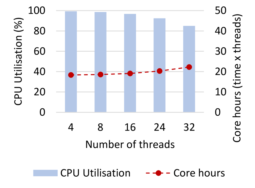
(b) CPU utilisation

Figure 7.9: Overall execution time and CPU utilisation when SLOW5 format is used

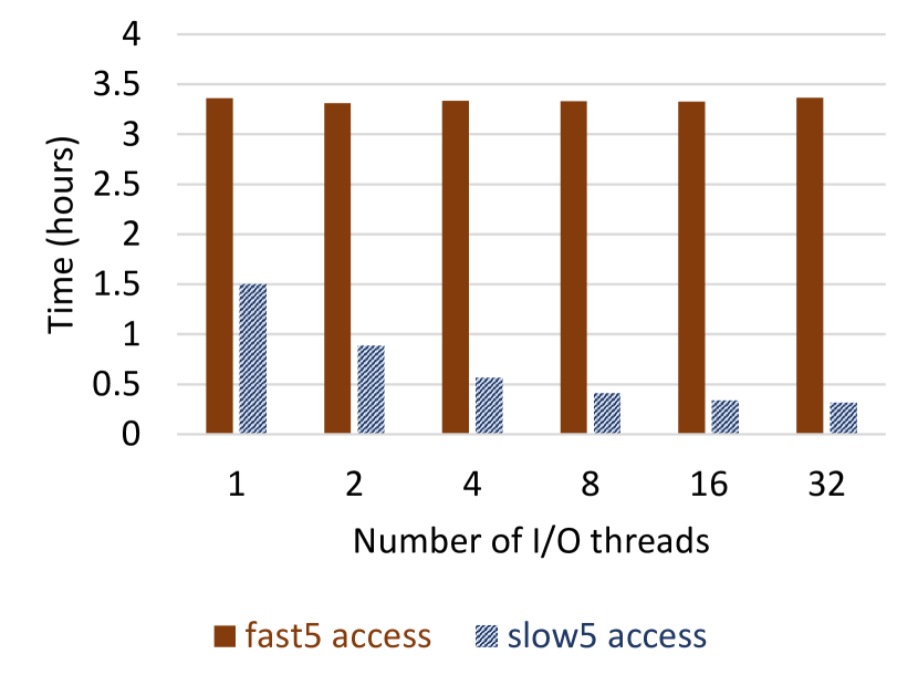
(a) On system S1: HDD RAID

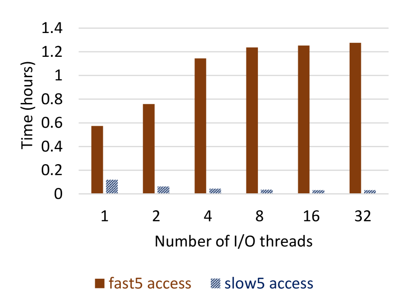
(b) On system S2: SSD RAID

Figure 7.10: Comparison of FAST5 vs SLOW5 access

I/O Time Consumption:

It was discussed previously that the identified bottleneck is due to I/O. Therefore, to get more insight into the effectiveness of our proposed solution, we plot and compare the time spent in I/O operations. Specifically, the time spent for reading nanopore raw signal data on system S1 when using SLOW5 format is compared to when using FAST5 format in Fig. 7.10(a). We make the following observations from the figure: 1) there is no improvement in FAST5 access time (brown bars) despite increasing the number of threads used (due to the lock in HDF5 library); 2) in contrast, there is a significant improvement for the proposed SLOW5 access time (blue bars) with the increased number of threads; and, 3) even at a single thread, the proposed SLOW5 is ${\sim}2\times$ times faster than FAST5, and at 32 threads the improvement of SLOW5 compared to FAST5 is ${\sim}10\times$. The speed-up in I/O time for the single thread is contributed by the exploitation of locality (discussed in Section 7.4.1) and our lightweight SLOW5 access implementation.

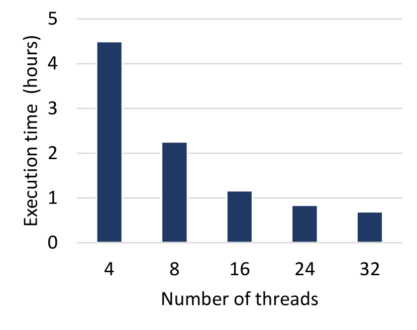
(a) Execution time

(b) CPU utilisation

Figure 7.11: Overall results for multi-process pool

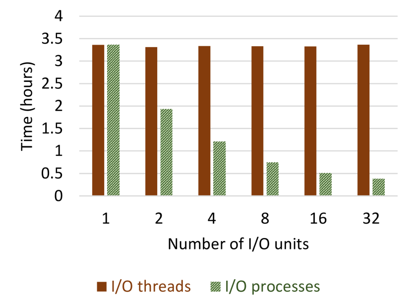
(a) On system S1: HDD RAID

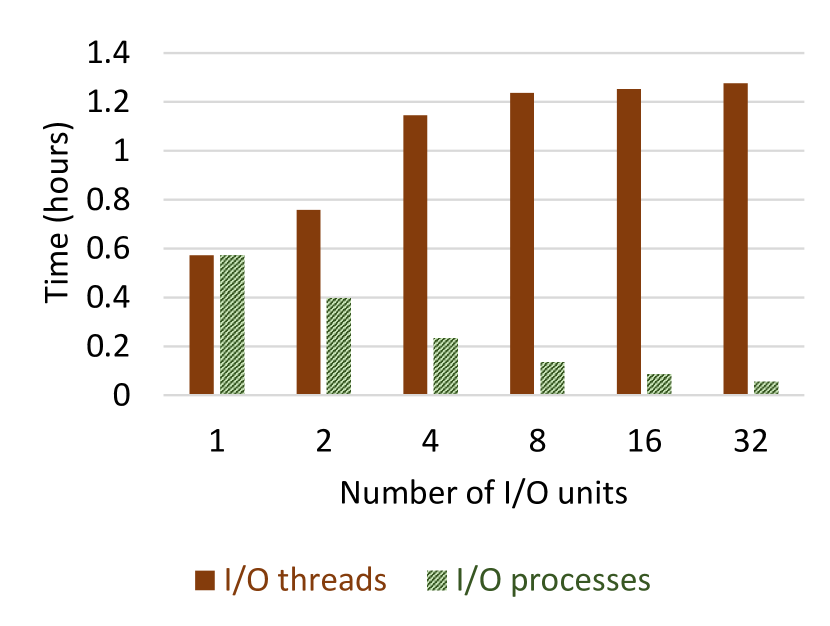
(b) On system S2: SSD RAID

Figure 7.12: FAST5 file access using multiple I/O threads vs I/O processes

Above experiments on system S1 demonstrated that our proposed solution effectively improves performance of Nanopolish. The S1 system consists of HDD RAID. Now, we demonstrate that our solution is also effective on SSD RAID using experiments on system S2. As discussed above, the I/O decomposition results are more insightful, therefore we present the I/O decomposition results on S2 system (SSD RAID based) for the sake of brevity of the manuscript. Fig. 7.10(b) shows the comparison of FAST5 access time to SLOW5 access time, where similar observations can be made. In fact, FAST5 access time (brown bars) got worse with the number of threads, whereas SLOW5 access time (blue bars) improved with the number of threads. At 32 threads SLOW5 was ${\sim}42\times$ faster than FAST5 on SSD RAID. Thus, our proposed solution is effective for the HDD based RAIDs as well as the SSD based RAIDs.

Note: The file sizes of the new SLOW5 format are comparable to the existing FAST5 format. Specifically, the dataset which was 845 GB in FAST5 format (Table 7.3), reduced to 340 GB when converted to SLOW5. The reduced size when converted to SLOW5 is due to storing global metadata in the header in SLOW5, instead of redundantly storing those for each read. SLOW5 index is quite small (47 MB) compared to gigabytes of RAM available on an HPC.

7.5.3 Results: Multi-process Pool

Overall Execution Time and CPU Utilisation: Overall execution time for the restructured and optimised Nanopolish when a multi-process pool is used for FAST5 access is shown in Fig. 7.11(a), whereas the CPU utilisation and the core-hours are depicted in Fig. 7.11(b). The x-axis of the figure corresponds to the number of data processing threads which is also equal to the number of I/O processes. The results in Fig. 7.11 are similar to that of the SLOW5 solution discussed in previous subsection. The key observations in Fig. 7.11 compared to original Nanopolish are also similar to the first solution. These are: 1) improved performance w.r.t. the original Nanopolish for a given number of threads; 2) improved CPU Utilisation; and, 3) better performance scaling with increasing number of threads, as depicted by the near-flat core-hour plot.

I/O Time Consumption: Similar to the previous section, we evaluate the time spent in I/O operations. We compare the results for the multi-threaded and the multi-process based versions. The plots are presented in Fig. 7.12, with the x-axis denoting the number of processes/threads used. On HDD RAID (Fig. 7.12(a)), the FAST5 access time does not improve with increased I/O threads (brown bars), while it significantly improves with increased I/O processes (green bars). At 32 threads/processes the improvement was ${\sim}9\times$. On SSD RAID (Fig. 7.12(b)), the FAST5 access time gets worse with increased I/O threads. In contrast, it significantly improves with increased I/O processes. Using 32 I/O processes is ${\sim}23\times$ faster than using 32 I/O threads on SSD RAID.

In summary, using processes instead of threads for I/O operations alleviates the I/O bottleneck, while using multiple-threads for data processing in a single parent-process avoids introduction of any additional significant bottlenecks, as depicted by the above results.

7.5.4 Comparison of SLOW5 to FAST5 with Multi-process Pool

Comparing the time for SLOW5 access in Fig. 7.10 with I/O process based pool for FAST5 (Fig. 7.12) shows that SLOW5 outperforms FAST5 even when multiple I/O processes are used especially at lower number of threads/processes.

7.5.5 Comparison with Multi-FAST5 Format

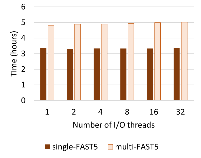
(a) On system S1: HDD RAID

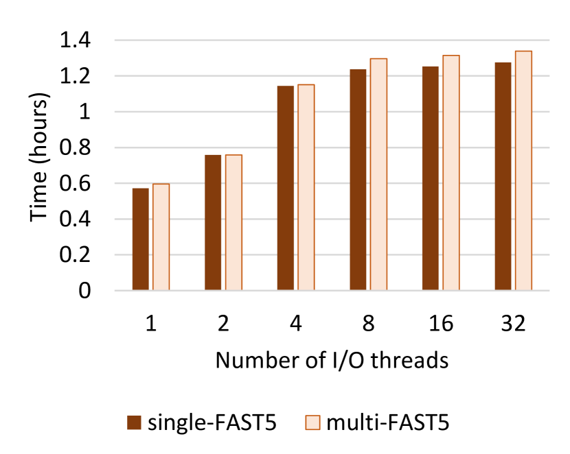
(b) On system S2: SSD RAID

Figure 7.13: Single-FAST5 vs Multi-FAST5 using I/O threads

ONT is recently working on a new file format: known as multi-FAST5. It is projected to replace the existing FAST5 format in near future. The raw signals from multiple genomic reads (by default 4000 genomic reads) are packed into a FAST5 file and such files are termed as multi-FAST5. Multi-FAST5 reduces the gigantic amount of small single-FAST5 files generated from a sequencing run, easing the file management (eg: copying/moving files, listing files). Multi-FAST5 files are also HDF5 files where the schema is an extended version for that of single-FAST5. Next, we demonstrate that multi-FAST5 suffers from a similar bottleneck, and thus our proposed SLOW5 is superior to the new multi-FAST5 format. Moreover, our multi-process based solution is also applicable and effective for multi-FAST5 format.

Performance Bottleneck in Multi-FAST5: First, we compare the file access time in multi-FAST5 to single-FAST5 in Fig. 7.13. Unfortunately, the access time does not improve by the use of multiple I/O threads on HDD RAID, similar to single-FAST5 (Fig. 7.13(a)). In fact, multi-FAST5 performance is actually worse than that of single-FAST5. On SSD RAID (Fig. 7.13(b)), the performance of multi-FAST5 and single-FAST5 are almost the same and gets gradually worse with the number of threads.

Proposed Multi-process Solution on Multi-FAST5: Now we demonstrate that our multi-process based solution is also applicable and effectively improves the performance for the new multi-FAST5 format. The access time for Multi-FAST5 and single-FAST5 with our multi-process solution for different number of threads are in Fig. 7.14. With our solution, the trend of multi-FAST5 access time is similar to that of single-FAST5 files (on both HDD RAID and SSD RAID), that is, it gets significantly better with the number of I/O processes used. Note that when the time with single-FAST5 is compared, multi-FAST5 takes more time than single FAST5, visibly in the HDD RAID.

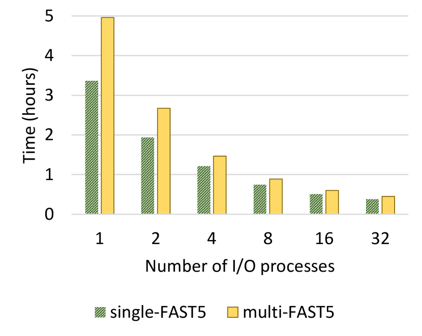
(a) On system S1: HDD RAID

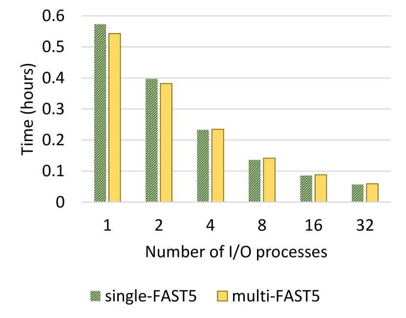
(b) On system S2: SSD RAID

Figure 7.14: Single-FAST5 vs Multi-FAST5 using I/O processes

7.5.6 On NFS

Our proposed optimisations has the potential to benefit direct execution of nanopore data analysis tools on data residing on a network attached storage. HPC cluster environments predominantly use such network attached storage in addition to local RAID systems. We demonstrate the performance of our proposed methods on NFS in Fig. 7.15.

Fig. 7.15(a) compares our SLOW5 format with FAST5 on NFS over multiple I/O threads. Use of multiple I/O threads for accessing FAST5 files on NFS (brown bars), slightly improves the performance up to around 4 threads (unlike previously on local RAID), which then saturates. SLOW5 access (blue bars) is much faster than FAST5. SLOW5 access time improves up to around 8 threads which then saturates.

Fig. 7.15(b) compares our proposed process pool based method to using multiple I/O threads. Use of multiple I/O processes (green bars) considerably improves the FAST5 access performance up to around 8 processes, which then slowly saturates, a similar trend to that with SLOW5. Comparing SLOW5 (blue bars in Fig. 7.15(a)) to FAST5 access using multiple I/O processes (Fig. 7.15(b)) shows that SLOW5 performance is superior.

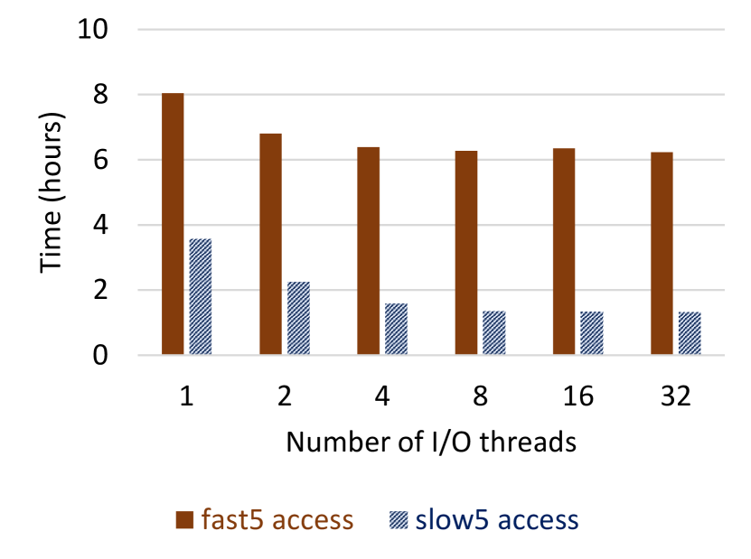
(a) SLOW5 performance on NFS

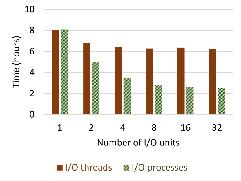
(b) FAST5 performance on NFS

Figure 7.15: Performance on NFS

Refer to appendix H for supplementary results and analyses.

7.6 Discussion

7.6.1 Other Possible Solutions

In this chapter, we presented two solutions to overcome the I/O bottleneck caused by the FAST5 file format and demonstrated their efficacy using experiments. Additionally, there are few other possible solutions to the problem, as discussed below.

Fixing HDF5 Library: As discussed above, using a new file format may not always be practical and we presented a multi-process based solution in such a scenario. Another candidate solution is to fix (optimise) the HDF5 library to be thread efficient. However, HDF5 library is a complicated library with a large code base of $>$300,000 lines of C code and such a fix has to be potentially done by the HDF Group [224, 225]. The HDF5 Group mentions that the future plan to implement efficient multi-threaded access is currently hindered by inadequate resources [236]. Therefore, such a fix is unlikely to happen in the near future. Moreover, there is no other alternate library to read HDF5 files[224, 225].

Naive Approaches of Multi-processing: Instead of using a process pool solely for FAST5 I/O and multi-threads for parallel data processing (as proposed in Section 7.4.2), programmers may use multi-processes for both the I/O operations and parallel data processing. This would be easier than implementing a pool of processes, however, this is only suitable for trivially parallel cases. If the application needs to share data among multiple processing units, processes are unsuitable due to the complexity that arise when performing inter-process communication.

Alternatively, the programmer may let users manually split data and launch multiple processes. Unfortunately, this method exerts additional burden on the user, i.e., custom scripts must be written for data splitting, launching data processing and concatenating the result. Moreover, this is only suitable for trivially parallel applications where data can be easily split. Also, an expensive HPC system with dozens of cores is superfluous as the user could use a cluster of low cost networked computers (as shown in chapter 6).

In summary, using processes instead of threads potentially solves the I/O bottleneck as we demonstrated in results. However, it is important to note that processes in an operating system are meant for isolation whereas threads are for sharing data. Inter-process communication requires system calls, while inter-thread communication involves sharing the same memory space. Further, processes are expensive to be spawned and are not lightweight (unlike threads). Thus, using processes as a replacement to threads makes the code relatively complicated. Therefore, we suggest that using the SLOW5 format is a superior solution than the multi-processes based solution.

7.6.2 Future Directions

As shown in section 7.5.2, SLOW5 file size is smaller than FAST5 due to the efficient storage of metadata. SLOW5 file size can potentially be further reduced by using a binary encoding instead of ASCII and/or by applying block compression techniques such as BGZF that still allows random access [239]. Having both ASCII and binary formats is useful, where the former is human readable and the latter is space efficient. In fact, gold standard file formats in genomics such as SAM and VCF that are in ASCII have their binary counterparts BAM and BCF.

After applying our proposed optimisations proposed in this chapter, the next bottleneck in Nanopolish could be the FASTA access (random access to reference genome) which is performed using the faidx component in htslib library. This faidx is not currently thread-safe and thus only single threaded access is possible. However, FASTA is a simple ASCII based format and thus extending faidx for thread efficiency is feasible as future work.

7.6.3 Potential Impact on other Toolkits and Domains

It is likely that the identified limitation in HDF5 libary is a primary bottleneck in several other nanopore software toolkits, which also use the HDF5 library such as Tombo [240], NanoMod [241] and SquiggleKit [242]. Thus, our proposed optimisations are potentially useful in such toolkits. Our work may also guide nanopore software developers to avoid the identified bottleneck in future. Furthermore, HDF5 is also used in other engineering domains such as physics, astronomy, weather forecasting [243]. Therefore, we believe that our work will inspire optimisations in those domains.

7.7 Summary

In this chapter, we demonstrated with an example that nanopore software fail to take maximal advantage of the computing power offered by many-core processors in HPC systems, despite multi-threaded implementation. To address this problem, we presented a systematic experimental analysis to identify potential performance bottlenecks in nanopore software tools for running on many-core CPUs. We identified that the bottleneck is caused by inefficient file I/O associated with the HDF5 library used for loading nanopore raw data. The inefficiency in file I/O in HDF5 is due to a global lock which limits multiple threads requesting file accesses in parallel. Then, we proposed multiple optimisations to alleviate the bottleneck. We proposed a new file format that facilitates efficient file access using multiple threads. For the scenarios where the original format must be used, we presented a multi-process based solution. Thus, our proposed optimisations can be used as an alternative, or alongside the existing file-format. Our experiments demonstrated that our optimisations not only enable improved performance for a given number of threads (${\sim}2\times$ for 4 threads and ${\sim}6.5\times$ for 32 threads), but also enable improved CPU utilisation (from 69% to 99% for 4 cores and from 22% to 85% for 32 threads) when compared to original Nanopolish. Consequently, improved performance scaling with the number of threads was also achieved (${\sim}6.5\times$ for 4 vs. 32 threads).

Chapter 8 Conclusion and Future Directions

DNA sequencing is a revolutionary technology that is reshaping the field of medicine and healthcare. In addition, DNA sequencing has important applications in other fields such as epidemiology and forensics. Over the last two decades, the size of DNA sequencers has shrunk from the size of a fridge to that of a mobile phone and sequencing cost per genome has remarkably reduced by more than 1000 times. These remarkable improvements are expected to continue further. Unfortunately, hundreds to thousands of gigabytes of data output from today’s ultra-portable sequencers is analysed on non-portable high-performance computers or cloud computers, which was the case even a couple of decades ago.

This thesis moved the DNA sequence analysis from high-performance computers to portable computing devices, a timely need for enhancing the use of ultra-portable sequencers in point-of-care or in-the-field. The objective was achieved using computer architecture-aware optimisation of complex DNA analysis workflows. Such optimisations enabled efficient mapping of the software to exploit complex features of modern computer hardware. Domain knowledge of both computer architecture and DNA sequence analysis was simultaneously used to achieve the twin goals of achieving efficient compute resource utilisation with no impact on accuracy. Therefore, this thesis is an attempt to bridge the two domains, DNA sequencing and computer architecture.

In this thesis, gold-standard DNA sequence analysis software tools were systematically examined for bottlenecks and architecture-aware optimisations were performed at I/O level, processor level, RAM level, cache level and at the register level. The optimised software tools were used to perform complete end-to-end analysis workflows on prototype embedded systems composed of single-board computers. The performance and accuracy were evaluated using real and representative datasets. The resultant embedded systems were fully functional with performance comparable to an unoptimised workflow on a high-performance computer. The constructed prototype embedded systems are currently being used for in-house data analysis at Garvan Institute of Medical Research, Sydney. Such low cost, energy-efficient, sufficiently fast and portable embedded system enables complete DNA analysis in point-of-care or in-the-field.

In addition to prototype embedded systems composed of single board computers, this thesis has also made it possible to run DNA analysis workflows on commodity portable computing devices such as laptops, tablets and mobile phones. The optimisations proposed in this thesis also benefit running DNA analysis workflows on high-performance computers through a magnitude of times faster performance. Optimised versions of software produced under the thesis are released as open-source software. The prototype embedded systems constructed under this thesis are fully functional that they are currently being used for in-house nanopore sequence data processing at Garvan Institute of Medical Research, Sydney. The open-source software produced under the thesis is being used by several research centres globally and users have surprised by the significant speedup achieved compared to existing software. The conclusion from each chapter of this thesis is given below.

A popular variant calling software for second-generation sequence data called Platypus was optimised for efficient usage of the memory hierarchy. Systematically examining the steps in variant calling revealed that 60% of the total variant calling time is consumed by de Bruijn graph construction during the local re-assembly step. After carefully inspecting the data access patterns, optimisations were proposed to improve the locality of memory accesses both at cache level and register level. The existing algorithm was modified to integrate the proposed optimisations, which in turn improved the efficient usage of faster cache memories and registers. The results showed that these changes improve the performance of de Bruijn graph construction by a factor of around two when implemented on a general-purpose processor. The modified algorithm opens the door to a much higher acceleration of local re-assembly on GPU, FPGA and ASIP. The implementation of the algorithm which is integrated into the Platypus Variant Caller is publicly available at https://github.com/hasindu2008/platycflr.

The gold standard software for aligning long reads generated from third-generation high-throughput sequencers called Minimap2 was optimised for removed memory capacity. Minimap2 relies on a large hash table data structure (constructed out of the reference genome) stored in RAM for the alignment process. Large reference genomes such as the human genome require 11GB for the hash table alone. Mere parameter optimisation in Minimap2 cannot substantially reduce memory usage without considerably sacrificing alignment quality. Memory capacity optimisations were proposed to substantially reduce memory usage. Memory capacity optimisations included partitioning an alignment index, saving the internal state, and merging the output a posteriori. This strategy reduced the memory requirements for aligning long reads to the human reference genome from 11GB to less than 2GB, with minimal impact on accuracy. This work made it possible to perform read alignment to large reference genomes using computers with limited volatile memory. The optimised version of Minimap2 is available as open-source at https://github.com/hasindu2008/minimap2-arm and is also integrated into the original Minimap2 software.

A popular signal analysis toolkit for analysing nanopore raw signal data called Nanopolish was optimised for CPU-GPU heterogeneous systems. Examining the methylation calling tool in the Nanopolish toolkit revealed that around 70% of the runtime is consumed by an algorithm called Adaptive Banded Event Alignment (ABEA). Despite this algorithm being not embarrassingly parallel, an approach was proposed that made this algorithm efficiently execute on GPUs. The high variability of the read lengths was one of the main challenges, which was remedied through a number of memory optimisations and a heterogeneous processing strategy that uses both CPU and GPU. Proposed optimisations yielded around 3-5$\times$ performance improvement on a CPU-GPU system when compared to a CPU. CPU-GPU optimised ABEA was integrated back into a completely re-engineered version of the Nanopolish methylation calling tool and this resultant new software was named f5c. It was demonstrated that f5c is adequately capable of processing data from a portable nanopore sequencer in real-time using an embedded SoC equipped with an ARM processor (with six cores) and NVIDIA GPU (256 cores). f5c not only benefits embedded SoC but also a wide range of systems equipped with GPUs from laptops to servers. f5c was not only around 9$\times$ faster on an HPC but also reduced the peak RAM by around 6$\times$ times. The source code of f5c is made available at https://github.com/hasindu2008/f5c.

A system architecture was proposed for performing a popular DNA methylation detection workflow on a prototype embedded system. The workflow was realised on the proposed architecture by integrating the optimised software versions from previous chapters. The proposed architecture was evaluated using off-the-shelf single-board computers and was demonstrated that performing real-time analysis of nanopore sequencing is possible on an embedded system. It was further demonstrated that the performance of the prototype embedded system is surprisingly similar to the performance on an HPC. The system architecture and the associated software for building a replica of the prototype are released and the open-source code is available at https://github.com/hasindu2008/nanopore-cluster and https://github.com/hasindu2008/f5p.

The cause behind the unexpected slow performance on an HPC was identified to be the Nanopore software failing to take maximal advantage of the computing power offered by many-core processors in HPC systems, despite its multi-threaded implementation. A systematic experimental analysis was conducted to identify potential performance bottlenecks in nanopore software tools for running on many-core CPUs. This analysis revealed that the bottleneck is caused by inefficient file I/O associated with the HDF5 library used for loading nanopore raw data. The inefficiency in file I/O in HDF5 was identified to be due to a global lock which limits multiple threads requesting file accesses in parallel. Multiple optimisations were proposed to alleviate the bottleneck: a new file format that facilitates efficient file access using multiple threads; and, a multi-process-based solution for the scenarios where the original format must be used. Thus, the proposed optimisations can be used as an alternative, or alongside the existing file-format. The experiments demonstrated that the optimisations not only enable improved performance for a given number of threads (${\sim}2\times$ for 4 threads and ${\sim}6.5\times$ for 32 threads) but also enable improved CPU utilisation (from 69% to 99% for 4 cores and from 22% to 85% for 32 threads) when compared to the original Nanopolish. Consequently, improved performance scaling with the number of threads was also achieved (${\sim}6.5\times$ for 4 vs. 32 threads).

Conclusively, the architecture-aware optimisations presented in this are significant contributions that result in an ultra-portable DNA analysis system which additionally benefit the performance of DNA analysis workflow on an HPC.

8.1 Future Directions

In the upcoming decades, DNA sequencers will further miniaturise and the sequencing cost will be increasingly affordable. Consequently, DNA tests have the potential to be routine and decentralised as are today’s blood tests. The realisation of this prospect requires sequence analysis devices also to be further miniaturised. This thesis has put the foundation by demonstrating functional complex DNA sequence analysis workflows on prototypical embedded systems constructed out of over-the-shelf embedded computing device. The goal was archived through architecture-aware optimisation of the analysis software, and with the future goal of building domain-specific architectures for DNA sequence analysis in mind.

The proposed architecture in this thesis was evaluated by a prototype constructed out of multiple single-board computers interconnected using Ethernet. The prototype is bulky, mainly due to many cables. However, designing a custom carrier board that can accommodate multiple off-the-shelf system-on-modules with integrated Ethernet and power delivery will produce a system that is many times smaller than the prototype. Besides, the proposed system can be miniaturised into a single chip by designing a multiprocessor system on a chip (MPSoC) composed of application-specific instruction-set processors (ASIP). Such an MPSoC will be a magnitude of times smaller, with superior performance and lower energy when compared to the current prototype. Such an MPSoC integrated into an ultra-portable sequencer will enable complete DNA analysis on the palmtop.

Orthogonal to the above directions, the currently developed embedded system can be extended to an end-to-end application of direct biological significance such as a diagnostic test. However, such a direction would require strong collaboration with biologists and clinicians. Furthermore, there are other branches in genomics that can be explored, for instance, Ribonucleic acid (RNA) workflows, meta-genomic analyses and de-novo assembly. As exemplified in this thesis for two DNA analysis workflows (genetic variant detection using second-generation sequencing and epigenetic modification detection using third-generation sequencing), the other workflows also will have significant room for improvement through architecture-aware optimisation alone. Increased collaboration between researchers from the two domains—computer architecture and DNA sequencing—will be favourable to efficiently reduce the gap between DNA sequencing analysis.

Appendix A Supplementary Materials - Featherweight Long Read Alignment using Partitioned Reference Indexes

  This appendix is published as supplementary material of [25] in Nature Scientific Reports under Creative Commons CC BY license.
 

A.1 Supplementary Note 1 - Detailed Methodology of the merging

This supplementary note elaborates the merging method in detail together with some implementation details.

A.1.1 Serialising (dumping) of the internal state

For each part of the partitioned index, a separate intermediate file (which we refer to as a dump) is created in the binary format [refer line 36-44 in https://github.com/hasindu2008/minimap2-arm/blob/v0.1-alpha/merge.c]. After a read is aligned to the partition of the index currently in memory, all the intermediate states for its alignments are dumped into this binary file [line 501-506 in https://github.com/hasindu2008/minimap2-arm/blob/v0.1-alpha/map.c]. Binary format was preferred as it reduces the file size compared to ASCII. When the last read is mapped to the current partition of the index in memory, the dump will contain the intermediate state of the mappings for all the reads, in the same order as the reads in the input read set. If the partitioned index had n partitions, at the end of the n^th partitions we will have n such dumps.

The dumped internal state includes; fifteen 32-bit unsigned integers (such as the reference ID, chaining scores, query and reference start and end), two 32-bit signed integers and one floating point value. All these information are inside a single structure in Minimap2 (called mm_reg1_t in minimap.h) which made the dumping convenient. The size required for a single alignment is around 80 bytes.

If the user has requested Minimap2 to generate the base-level alignment, then the internal state for base-level alignment are also dumped. Base-level alignment information include; six 32-bit integers (such as the base level alignment score, number of CIGAR operations and a variable size flexible integer array for storing CIGAR operations. These information are stored inside another structure in Minimap2 (called mm_extra_t), which is only allocated if the base level alignment has been requested. The memory address to this structure is stored as a pointer in the previously mentioned mm_reg1_t structure. When dumping, we flatten the information linearly (eliminate memory pointers) to the file.

In addition to the above, a quantity called replen (sum of lengths of regions in the read that are covered by highly repetitive k-mers) is dumped. This is a per read quantity. We save the replen to the same dump file that we discussed above, just after the information for each mapping. For each read there will be a replen for each part of the index, that is saved in the dump for that particular part of the partitioned index [line 495 of https://github.com/hasindu2008/minimap2-arm/blob/v0.1-alpha/map.c].

A.1.2 Merging operation

When alignment of all reads to all parts of the index completes, the merging operation is invoked [merge function in https://github.com/hasindu2008/minimap2-arm/blob/v0.1-alpha/merge.c]. We simultaneous open the read file and the dump files for all parts of the partitioned index. Reads are sequentially loaded while loading all the internal states for the alignments of that read. This includes the internal state for all its alignments (includes the base-level information if it had been requested) as well as the replen from each dump file. The flattened data in the files are restored to their original structures when loading to the memory.

If no base-level alignments had been requested, the alignments are sorted based on the chaining score in descending order [function mm_hit_sort_by_score in https://github.com/hasindu2008/minimap2-arm/blob/v0.1-alpha/merge.c]. If base-level alignment had been requested, they are sorted based on the base-level DP alignment score. Categorisation of primary and secondary chains is performed on the sorted alignments according to the same method done on Minimap2 (using mm_set_parent function). This fixes the issue with the primary vs secondary flag. Then the alignment entries are filtered based on the user requested number of secondary alignments and the priority ratio (using mm_select_sub function). This eliminates the issue of outputting secondary alignments for each part of the index that makes the output size huge. If the output has been requested in form of a SAM file, the best primary alignment is set to the primary flag while all other primary alignments are set to supplementary (using mm_set_sam_pri function).

The mapping quality (MAPQ) estimation depends on the length of the read covered by repeat regions in the genome. To compute a perfect value for this quantity, the whole index needs to be in the memory which is the case for a single reference index. However, we estimate this quantity by taking the maximum out of the replen values that were dumped for the particular read. The Spearman correlation of this estimated value to the perfect replen was 0.9961. As the mapping quality is anyway an estimation, computing the mapping quality based on the estimated replen does not affect the final results significantly.

A.1.3 Emulated single reference index

For memory efficiency, Minimap2 stores meta-data of reference sequences (such as the sequence name and sequence length) only in the reference index (refer to mm_idx_t struct in minimap.h). The order in which the sequences reside in the struct array forms a unique numeric identifier for each reference sequence.

In the internal state for mappings only this numeric identifier is stored. The meta-data for the reference sequence are resolved using these numeric identifiers, only during the output printing. However, during merging we do not have the reference indexes in memory and the numeric identifiers cannot be resolved. Hence, we construct an emulated single reference index. For this, we save the meta-data of the reference sequences when each part of the partitioned index is loaded [line 47-54 in https://github.com/hasindu2008/minimap2-arm/blob/v0.1-alpha/merge.c]. These meta-data go to the beginning of the dump file for the particular part of the index. At the beginning of the merging, the meta-data is loaded back to form an emulated single reference index [line 164-173 in https://github.com/hasindu2008/minimap2-arm/blob/v0.1-alpha/merge.c]. However, the numeric identifiers in the internal states from the dump files are incorrect (as numeric the identifier is an independent incrementing index for each part of the index). These are corrected to be compatible with the numeric identifiers in the emulated single reference index by adding the correct offset [line 254 in https://github.com/hasindu2008/minimap2-arm/blob/v0.1-alpha/merge.c].

As a side effect of this emulated single reference index, a correct SAM header can be output even in the partitioned mode. Further, the merging process which merges the mappings for a read at a time, outputs the mappings for a particular read ID adjacently. Hence, no additional sorting is required for any downstream analysis tools that require so.

A.2 Supplementary Note 2 - Detailed Methodology of the chromosome balancing

A.2.1 Memory efficiency for references with unbalanced lengths

The existing partitioned index construction method in Minimap2, does not balance the size of index partitions when the reference genome has sequences (chromosomes) with highly varying lengths. This existing index construction method puts the reference sequences to the index in the order they exist in the reference genome. When constructing a partitioned index, it moves to the next part of of the index only when the user specified number of bases per index (by default 4 Gbases) is exceeded. When building a partitioned index for overlap finding, the parts would be approximately equal in size as the length of the longest read would be a few mega bases. However, in case of a reference genomes like the human genome where the chromosomes are of highly variable lengths, the size of the parts are unbalanced. The largest part of the index determines the peak memory. Hence, an unbalance will hinder the maximum efficiency for systems with limited memory. For instance, consider a hypothetical genome (total length 700M) with following chromosomes and lengths in the order chr1 (300M), chr2 (320M), chr3 (60M), chr4 (20M). Providing a value of 350M as the number of bases in a partition (with the intention of splitting into 2 parts), will create an unbalanced index as follows.

• part1 : chr1, chr2 : total length - 620M

• part2 : chr3, chr4 : total length - 80M

We follow a simple partitioning approach to balance this out. Instead of the number of bases per partition, the number of partitions is taken as a user input. The reference sequences are first sorted in descending order based on the sequence length (length without the ambiguous N bases). The sum of bases in each partition is initialised to 0. The, the sorted list in traversed in order while assigning the current sequence into the partition with the minimum sum of bases. The sum of bases in that partition is updated accordingly. Using this strategy, we get a distribution as follows.

• part1 : 300M, 60M : total length - 360M

• part2 : 320M, 20M : total length - 340M

A.3 Supplementary Note 3 - Instructions to run the tools

A.3.1 Example

1. Download and compile minimap2 that supports partitioned indexes and merging

   ⬇

   1wget https://github.com/hasindu2008/minimap2-arm/archive/v0.1.tar.gz

   2tar xvf v0.1.tar.gz && cd minimap2-arm-0.1 && make

2. Download the human reference genome and create a partitioned index with 4 partitions

   ⬇

   1wget -O hg38noAlt.fa.gz http://bit.ly/hg38noAlt && gunzip hg38noAlt.fa.gz

   2./misc/idxtools/divide_and_index.sh hg38noAlt.fa 4 hg38noAlt.idx ./minimap2 map-ont

   Note : http://bit.ly/hg38noAlt redirects to
   ftp://ftp.ncbi.nlm.nih.gov/genomes/all/GCA/000/001/405/GCA_000001405.15_GRCh38/seqs_for_alignment_pipelines.ucsc_ids/GCA_000001405.15_GRCh38_no_alt_analysis_set.fna.gz

3. Download a Nanopore NA12878 dataset and run Minimap2 with merging

   ⬇

   1wget -O na12878.fq.gz http://bit.ly/NA12878

   2./minimap2 -a -x map-ont hg38noAlt.idx na12878.fq.gz --multi-prefix tmp > out.sam

   Note : http://bit.ly/NA12878 redirects to
   http://s3.amazonaws.com/nanopore-human-wgs/rel3-nanopore-wgs-84868110-FAF01132.fastq.gz

Notes :

• To perform mapping without base-level alignment use:

  ⬇

  1./minimap2 -x map-ont hg38noAlt.idx na12878.fq.gz --multi-prefix tmp > out.paf

• From Minimap2 version 2.12-r827 [https://github.com/lh3/minimap2/blob/master/NEWS.md#release-212-r827-6-august-2018] onwards, the merging functionality has been integrated into the main repository. This version additionally supports paired-end short reads and the merging operation is multi-threaded. Use --split-prefix option instead of --multi-prefix.

A.3.2 Index construction with chromosome size balancing

divide_and_index.sh is the wrapper script for balanced index construction. It takes the reference genome and outputs a partitioned index optimised for reduced peak memory. Its usage is as follows:

⬇

1usage : ./divide_and_index.sh <reference.fa> <num_parts> <out.idx> <minimap2_exe>

2<minimap2_profile>

3

4reference.fa - path to the fasta file containing the reference genome

5num_parts - number of partitions in the index

6out.idx - path to the file to which the index should be dumped

7minimap2_exe - path to the minimap2 executable

8minimap2_profile - minimap2 pre-set for indexing (map-pb or map-ont)

9

10Example : ./divide_and_index.sh hg19.fa 4 hg19.idx minimap2 map-ont

Functionality of divide_and_index.sh is as follows.

1. Compiling divide.c using gcc to produce divide.

2. Calling the compiled binary divide to split the reference genome into partitions such that the total length of chromosomes in each partition are approximately equal.

3. Calling the minimap2 binary separately on each reference partition to produce a separate index file for each partition.

4. Combining all the index files to produce a single partitioned index file.

A.3.3 Running Minimap2 on a partitioned index with merging

To run minimap2 on an index created using the above method :

⬇

1minimap2 -x <profile> <partioned_index.idx> <reads.fastq> --multi-prefix <tmp-prefix>

--multi-prefix which takes a prefix for temporary files, enables the merging of the outputs generated through iterative mapping to index partitions.

Appendix B Appendix: f5c Documentation

  This appendix is based on the f5c documentation available at https://hasindu2008.github.io/f5c associated with the GitHub repository at https://github.com/hasindu2008/f5c.
 

B.1 Readme

f5c is an optimised re-implementation of the call-methylation and eventalign modules in Nanopolish. Given a set of basecalled Nanopore reads and the raw signals, f5c call-methylation detects the methylated cytosine and f5c eventalign aligns raw nanopore DNA signals (events) to the base-called read. f5c can optionally utilise NVIDIA graphics cards for acceleration.

First, the reads have to be indexed using f5c index. Then, invoke f5c call-methylation to detect methylated cytosine bases. Finally, you may use f5c meth-freq to obtain methylation frequencies. Alternatively, invoke f5c eventalign to perform event alignment. The results are almost the same as from nanopolish except for a few differences due to floating point approximations.

Full Documentation : https://hasindu2008.github.io/f5c/docs/overview

Pre-print : https://doi.org/10.1101/756122

B.1.1 Quick start

If you are a Linux user and want to quickly try out, download the compiled binaries from the latest release. For example:

⬇

1VERSION=v0.4

2wget "https://github.com/hasindu2008/f5c/releases/download/$VERSION/f5c-$VERSION-binaries.tar.gz" && tar xvf f5c-$VERSION-binaries.tar.gz && cd f5c-$VERSION/

3./f5c_x86_64_linux # CPU version

4./f5c_x86_64_linux_cuda # cuda supported version

Binaries should work on most Linux distributions and the only dependency is zlib which is available by default on most distros.

B.1.2 Building

Users are recommended to build from the latest release tar ball. You need a compiler that supports C++11. Quick example for Ubuntu :

⬇

1sudo apt-get install libhdf5-dev zlib1g-dev #install HDF5 and zlib development libraries

2VERSION=v0.4

3wget "https://github.com/hasindu2008/f5c/releases/download/$VERSION/f5c-$VERSION-release.tar.gz" && tar xvf f5c-$VERSION-release.tar.gz && cd f5c-$VERSION/

4scripts/install-hts.sh # download and compile the htslib

5./configure

6make # make cuda=1 to enable CUDA support

The commands to install hdf5 (and zlib) development libraries on some popular distributions :

⬇

1On Debian/Ubuntu : sudo apt-get install libhdf5-dev zlib1g-dev

2On Fedora/CentOS : sudo dnf/yum install hdf5-devel zlib-devel

3On Arch Linux: sudo pacman -S hdf5

4On OS X : brew install hdf5

If you skip scripts/install-hts.sh and ./configure hdf5 will be compiled locally. It is a good option if you cannot install hdf5 library system wide. However, building hdf5 takes ages.

Building from the Github repository additionally requires autoreconf which can be installed on Ubuntu using sudo apt-get install autoconf automake.

Other building options are detailed in section B.2.Instructions to build a docker image is detailed section B.2.4.

B.1.2.1 NVIDIA CUDA support

To build for the GPU, you need to have the CUDA toolkit installed. Make sure nvcc (NVIDIA C Compiler) is in your PATH.

The building instructions are the same as above, except that you should call make as :

⬇

1make cuda=1

Optionally you can provide the CUDA architecture as :

⬇

1make cuda=1 CUDA_ARCH=-arch=sm_xy

If your CUDA library is not in the default location /usr/local/cuda/lib64, point to the correct location as:

⬇

1make cuda=1 CUDA_LIB=/path/to/cuda/library/

Refer to section B.2.5 for troubleshooting CUDA related problems.

B.1.3 Usage

⬇

1f5c index -d [fast5_folder] [read.fastq|fasta]

2f5c call-methylation -b [reads.sorted.bam] -g [ref.fa] -r [reads.fastq|fasta] > [meth.tsv]

3f5c meth-freq -i [meth.tsv] > [freq.tsv]

4f5c eventalign -b [reads.sorted.bam] -g [ref.fa] -r [reads.fastq|fasta] > [events.tsv]

Refer to section B.2.8 for all the commands and options.

B.1.3.1 Example

Follow the same steps as in Nanopolish tutorial while replacing nanopolish with f5c. If you only want to perform a quick test of f5c :

⬇

1#download and extract the dataset including sorted alignments

2wget -O f5c_na12878_test.tgz "https://f5c.page.link/f5c_na12878_test"

3tar xf f5c_na12878_test.tgz

4

5#index, call methylation and get methylation frequencies

6f5c index -d chr22_meth_example/fast5_files chr22_meth_example/reads.fastq

7f5c call-methylation -b chr22_meth_example/reads.sorted.bam -g chr22_meth_example/humangenome.fa -r chr22_meth_example/reads.fastq > chr22_meth_example/result.tsv

8f5c meth-freq -i chr22_meth_example/result.tsv > chr22_meth_example/freq.tsv

9#event alignment

10f5c eventalign -b chr22_meth_example/reads.sorted.bam -g chr22_meth_example/humangenome.fa -r chr22_meth_example/reads.fastq > chr22_meth_example/events.tsv

B.1.4 Acknowledgement

This repository reuses code and methods from Nanopolish. The event detection code is from Oxford Nanopore’s Scrappie basecaller. Some code snippets have been taken from Minimap2 and Samtools.

B.2 Building f5c

Note : Building from the Github repository requires autoreconf which can be installed on Ubuntu using sudo apt-get install autoconf automake.

Clone the git repository.

⬇

1git clone https://github.com/hasindu2008/f5c && cd f5c

Alternatively, download the latest release tarball and extract. eg :

⬇

1VERSION=v0.4

2wget "https://github.com/hasindu2008/f5c/releases/download/$VERSION/f5c-$VERSION-release.tar.gz" && tar xvf f5c-$VERSION-release.tar.gz && cd f5c-$VERSION/

While we have tried hard to avoid the dependency hell, three dependencies (zlib, HDF5 and HTS) could not be avoided.

Currently 3 building methods are supported.

1. Locally compiled HTS library and system wide HDF5 library (recommended).

2. Locally compiled HTS and HDF5 libraries (HDF5 local compilation - takes a bit of time).

3. System wide HTS and HDF5 libraries (not recommended as HTS versions can be old).

B.2.1 Method 1 (recommended)

Dependencies : Install the HDF5 (and zlib development libraries).

⬇

1On Debian/Ubuntu : sudo apt-get install libhdf5-dev zlib1g-dev

2On Fedora/CentOS : sudo dnf/yum install hdf5-devel zlib-devel

3On Arch Linux: sudo pacman -S hdf5

4On OS X : brew install hdf5

Now build f5c.

⬇

1autoreconf # skip if compiling a release, only required when building from github

2scripts/install-hts.sh # download and compiles htslib in the current folder

3./configure

4make # or make cuda=1 if compiling for CUDA

B.2.2 Method 2 (time consuming)

Dependencies : Install the zlib development libraries.

⬇

1On Debian/Ubuntu : sudo apt-get install zlib1g-dev

2On Fedora/CentOS : sudo dnf/yum install zlib-devel

Now build f5c.

⬇

1autoreconf # skip if compiling a release, only required when building from github

2scripts/install-hts.sh # download and compiles htslib in the current folder

3scripts/install-hdf5.sh # download and compiles HDF5 in the current folder

4./configure --enable-localhdf5

5make # or make cuda=1 if compiling for CUDA

B.2.3 Method 3 (not recommended)

Dependencies : Install HDF5 and hts.

⬇

1On Debian/Ubuntu : sudo apt-get install libhdf5-dev zlib1g-dev libhts1

Now build f5c.

⬇

1autoreconf # skip if compiling a release, only required when building from github

2./configure --enable-systemhts

3make # or make cuda=1 if compiling for CUDA

B.2.4 Docker Image

To build a docker image:

⬇

1git clone https://github.com/hasindu2008/f5c && cd f5c

2docker build .

Note down the image uuid and run f5c as:

⬇

1docker run -v /path/to/local/data/data/:/data/ -it :image_id ./f5c call-methylation -r /data/reads.fa -b /data/alignments.sorted.bam -g /data/ref.fa

B.2.5 CUDA Troubleshooting

B.2.6 Compiling Issues

B.2.6.1 make: nvcc: Command not found error when I compile with make cuda=1

Make sure that the NVIDIA CUDA toolkit is installed. See instruction at the official installation guide. If you still get this error after the toolkit installation, then nvcc is probably not in your PATH. In that case, either add the nvcc location to your PATH or manually specify the nvcc location through a Makefile variable.

Example:

If you installed the CUDA toolkit through apt in Ubuntu,

⬇

1make cuda=1 NVCC=/usr/local/cuda/bin/nvcc

If you did the Runfile installation on Ubuntu,

⬇

1make cuda=1 NVCC=/usr/local/cuda-<toolkit-version>/bin/nvcc

Note that the location of nvcc might be different depending on your distribution and the installation method.

B.2.6.2 Cannot find -lcudart_static error.

The default CUDA library path in the Makefile is set to be /usr/local/cuda/lib64.

While this is the default path for an Ubuntu 64-bit system with the CUDA toolkit installed using the package manager apt, it might be different on your system. You can manually specify the path to the cuda library when compiling.

Example:

If you did the Runfile installation on Ubuntu,

⬇

1make cuda=1 CUDA_LIB=/usr/local/cuda-<toolkit-version>/lib64/

If you are using Ubuntu 32-bit,

⬇

1make cuda=1 CUDA_LIB=/usr/local/cuda/lib/

Note that the location of the CUDA library path might be different depending on your distribution and the installation method.

B.2.6.3 memcpy was not declared in this scope error

If you get an error like this:

⬇

1$ make cuda=1

2nvcc -x cu -g -O2 -std=c++11 -lineinfo -Xcompiler -Wall -I./htslib -DHAVE_CUDA=1 -rdc=true -c src/f5c.cu -o build/f5c_cuda.o

3/usr/include/string.h: In function ’void* __mempcpy_inline(void*, const void*, size_t)’:

4/usr/include/string.h:652:42: error: ’memcpy’ was not declared in this scope

5return (char *) memcpy (__dest, __src, __n) + __n;

6^

7Makefile:76: recipe for target ’build/f5c_cuda.o’ failed

8make: *** [build/f5c_cuda.o] Error 1

Compile with -D_FORCE_INLINES appended to CUDA_CFLAGS when calling make:

⬇

1CUDA_CFLAGS+="-D_FORCE_INLINES" make cuda=1

The issue is reported in #36. And this fix is suggested in opencv/opencv#6500.

B.2.7 Runtime Errors

B.2.7.1 CUDA driver version is insufficient for CUDA runtime version

Check the following in order:

1. Do you have an NVIDIA GPU / is your NVIDIA GPU recognised by the system?
   On most distributions you can use the following command to verify:

   ⬇

   1lspci | grep -i "vga\|3d\|display"

   It should list the NVIDIA GPU:

   ⬇

   101:00.0 3D controller: NVIDIA Corporation GP107M [GeForce GTX 1050 Ti Mobile] (rev a1)

2. Have you installed the NVIDIA driver (not the open source nouveau driver)?
   On most distributions you can check your graphics card driver using

   ⬇

   1lspci -nnk | grep -iA2 "vga\|3d\|display"

   If the kernel driver output contains nvidia, then you are using the correct driver.

   ⬇

   101:00.0 3D controller [0302]: NVIDIA Corporation GP107M [GeForce GTX 1050 Ti Mobile] [10de:1c8c] (rev a1)

   2 Kernel driver in use: nvidia

   3 Kernel modules: nvidiafb, nouveau, nvidia_396, nvidia_396_drm

3. If you are using a Tegra GPU (e.g. Jetson TX2), does the current user belong to the “video” user group?
   Check the current group names with group [user].
   

4. Is the CUDA driver version too old for the toolkit that is used to compile with?
   See the cuda binary compatibility guide.
   The release CUDA binary that we provide is compiled using CUDA toolkit 6.5. The CUDA runtime library is statically linked and therefore release CUDA binaries work on driver version >= 340.21.
   Use nvidia-smi to check your driver version.

   ⬇

   1$ nvidia-smi

   2+-----------------------------------------------------------------------------+

   3| NVIDIA-SMI 396.44 Driver Version: 396.44 |

   If you compiled the binary yourself, see the cuda binary compatibility guide to check if your toolkit version and driver version match.

B.2.8 Commands and options

B.2.9 Available f5c tools

⬇

1Usage: f5c <command> [options]

2

3command:

4 index Build an index mapping from basecalled reads to the signals measured by the sequencer (same as nanopolish index)

5 call-methylation Classify nucleotides as methylated or not (optimised nanopolish call-methylation)

6 meth-freq Calculate methylation frequency at genomic CpG sites (optimised nanopolish calculate_methylation_frequency.py)

7 eventalign Align nanopore events to reference k-mers (optimised nanopolish eventalign)

B.2.9.1 Indexing

⬇

1Usage: f5c index [OPTIONS] -d nanopore_raw_file_directory reads.fastq

2Build an index mapping from basecalled reads to the signals measured by the sequencer

3f5c index is equivalent to nanopolish index by Jared Simpson

4

5 -h, --help display this help and exit

6 -v, --verbose display verbose output

7 -d, --directory path to the directory containing the raw ONT signal files. This option can be given multiple times.

8 -s, --sequencing-summary the sequencing summary file from albacore, providing this option will make indexing much faster

9 -f, --summary-fofn file containing the paths to the sequencing summary files (one per line)

B.2.9.2 Calling methylation

⬇

1Usage: f5c call-methylation [OPTIONS] -r reads.fa -b alignments.bam -g genome.fa

2 -r FILE fastq/fasta read file

3 -b FILE sorted bam file

4 -g FILE reference genome

5 -w STR[chr:start-end] limit processing to genomic region STR

6 -t INT number of threads [8]

7 -K INT batch size (max number of reads loaded at once) [512]

8 -B FLOAT[K/M/G] max number of bases loaded at once [2.0M]

9 -h help

10 -o FILE output to file [stdout]

11 --iop INT number of I/O processes to read fast5 files [1]

12 --min-mapq INT minimum mapping quality [30]

13 --secondary=yes|no consider secondary mappings or not [no]

14 --verbose INT verbosity level [0]

15 --version print version

16 --disable-cuda=yes|no disable running on CUDA [no]

17 --cuda-dev-id INT CUDA device ID to run kernels on [0]

18 --cuda-max-lf FLOAT reads with length <= cuda-max-lf*avg_readlen on GPU, rest on CPU [3.0]

19 --cuda-avg-epk FLOAT average number of events per kmer - for allocating GPU arrays [2.0]

20 --cuda-max-epk FLOAT reads with events per kmer <= cuda_max_epk on GPU, rest on CPU [5.0]

21 -x STRING profile to be used for optimal CUDA parameter selection. user-specified parameters will override profile values

22advanced options:

23 --kmer-model FILE custom k-mer model file

24 --skip-unreadable=yes|no skip any unreadable fast5 or terminate program [yes]

25 --print-events=yes|no prints the event table

26 --print-banded-aln=yes|no prints the event alignment

27 --print-scaling=yes|no prints the estimated scalings

28 --print-raw=yes|no prints the raw signal

29 --debug-break [INT] break after processing the specified batch

30 --profile-cpu=yes|no process section by section (used for profiling on CPU)

31 --skip-ultra FILE skip ultra long reads and write those entries to the bam file provided as the argument

32 --ultra-thresh [INT] threshold to skip ultra long reads [100000]

33 --write-dump=yes|no write the fast5 dump to a file or not

34 --read-dump=yes|no read from a fast5 dump file or not

35 --meth-out-version [INT] methylation tsv output version (set 2 to print the strand column) [1]

36 --cuda-mem-frac FLOAT Fraction of free GPU memory to allocate [0.9 (0.7 for tegra)]

B.2.9.3 Calculate methylation frequency

⬇

1Usage: meth-freq [options...]

2

3 -c [float] Call threshold. Default is 2.5.

4 -i [file] Input file. Read from stdin if not specified.

5 -o [file] Output file. Write to stdout if not specified.

6 -s Split groups

B.2.9.4 Aligning events

⬇

1Usage: f5c eventalign [OPTIONS] -r reads.fa -b alignments.bam -g genome.fa

2 -r FILE fastq/fasta read file

3 -b FILE sorted bam file

4 -g FILE reference genome

5 -w STR[chr:start-end] limit processing to genomic region STR

6 -t INT number of threads [8]

7 -K INT batch size (max number of reads loaded at once) [512]

8 -B FLOAT[K/M/G] max number of bases loaded at once [2.0M]

9 -h help

10 -o FILE output to file [stdout]

11 --iop INT number of I/O processes to read fast5 files [1]

12 --min-mapq INT minimum mapping quality [30]

13 --secondary=yes|no consider secondary mappings or not [no]

14 --verbose INT verbosity level [0]

15 --version print version

16 --disable-cuda=yes|no disable running on CUDA [no]

17 --cuda-dev-id INT CUDA device ID to run kernels on [0]

18 --cuda-max-lf FLOAT reads with length <= cuda-max-lf*avg_readlen on GPU, rest on CPU [3.0]

19 --cuda-avg-epk FLOAT average number of events per kmer - for allocating GPU arrays [2.0]

20 --cuda-max-epk FLOAT reads with events per kmer <= cuda_max_epk on GPU, rest on CPU [5.0]

21 -x STRING profile to be used for optimal CUDA parameter selection. user-specified parameters will override profile values

22advanced options:

23 --kmer-model FILE custom k-mer model file

24 --skip-unreadable=yes|no skip any unreadable fast5 or terminate program [yes]

25 --print-events=yes|no prints the event table

26 --print-banded-aln=yes|no prints the event alignment

27 --print-scaling=yes|no prints the estimated scalings

28 --print-raw=yes|no prints the raw signal

29 --debug-break [INT] break after processing the specified batch

30 --profile-cpu=yes|no process section by section (used for profiling on CPU)

31 --skip-ultra FILE skip ultra long reads and write those entries to the bam file provided as the argument

32 --ultra-thresh [INT] threshold to skip ultra long reads [100000]

33 --write-dump=yes|no write the fast5 dump to a file or not

34 --read-dump=yes|no read from a fast5 dump file or not

35 --summary FILE summarise the alignment of each read/strand in FILE

36 --sam write output in SAM format

37 --print-read-names print read names instead of indexes

38 --scale-events scale events to the model, rather than vice-versa

39 --samples write the raw samples for the event to the tsv output

40 --cuda-mem-frac FLOAT Fraction of free GPU memory to allocate [0.9 (0.7 for tegra)]

Appendix C Supplementary Materials - f5c

C.1 Why Nanopolish had to be re-engineered?

There are three reasons why Nanopolish had to be completely re-engineered into f5c for a successful GPU implementation.

• Nanopolish performs on-demand loading of signal data from file (a CPU thread assigned to the particular read invokes a file access just prior to signal alignment). However, transferring read by read to the GPU will incur a massive penalty and thus a batch of reads have to be transferred at once. Thus, we had to re-write the Nanopolish processing framework in such a way that loading and processing of a batch are performed batch wise. In f5c, we read a batch of data to the RAM and then bulk transfer to GPU memory, a batch of n reads at a time.

• Nanopolish thread model un-suitable for GPU acceleration—a thread is dynamically assigned to a read using openMP, thus each read has its own code path. However, offloading a batch of reads to the GPU for signal alignment requires code paths of all the reads in the batch to have converged before the GPU kernel is invoked. In addition, accurately measuring time, benchmarking and profiling of individual algorithmic components is hindered by such divergent code paths. pthread based approach that interleaves input reading, processing and output.

• Nanopolish is not optimised for efficient resource utilisation (eg: marginal performance improvement beyond 16 threads on servers and heavy-weight for embedded systems due to spurious malloc calls). A comparison of such a version with the GPU would result in an apparent high speedup, which is unfair.

C.2 Additional advantages of f5c over Nanopolish

In addition to the GPU acceleration of ABEA, f5c has many additional advantages over original Nanopolish.

• I/O and processing are interleaved in f5c: the I/O latency is considerably minimised.

• Our CPU version alone is around 1.5X-2X faster than the Nanopolish call methylation implementation and is very lightweight - suitable for embedded systems due to the careful use of data structures and algorithms.

• f5c is capable of detecting load balance problems between CPU and GPU, and report user with suggestion for appropriate parameters.

• f5c works with package manager’s system wide installations of HDF5 (no need of thread-safe build of HDF5), hence no need locally compile HDF5.

• Dependency hell has been minimised for both CPU and GPU versions. Compatible with g++ 4.8 or higher, and CUDA toolkit 6.5 or higher.

• f5c has suggestive error message for troubleshooting, especially the issues with respect to GPU.

• Pthread based thread framework written in C that interleaves I/O with processing is very lightweight and can be a starting point for future Nanopore tools.

• f5c allows benchmarking section by section to identify the bottlenecks in performance.

• f5c framework is suitable for the acceleration of core kernels through other methods such as FPGA.

Appendix D Generating portable binaries for ONT tools

  This appendix is based on a blog article published at https://hasindu2008.github.io/portable-binary.
 

Compiling software can sometimes be a nightmare due to numerous dependencies. This is specifically the case for bioinformatics tools that utilise signal level data from Oxford Nanopore (ONT) sequencers. According to my experience, the major cause behind compilation troubles in ONT tools is the Hierarchical Data Format 5 (HDF5) library. While a system admin may enjoy tedious compilations, it is not the case for users of bioinformatics tools. What if the tool developers release pre-compiled binaries? Some would object this as it is not a perfect solution. Nevertheless, I believe that it is far better than releasing an unusable tool due to users giving up at the compilation stage. Further, pre-compiled binaries are less bulky compared to docker images. Generating a “portable binary” that runs on numerous Linux distributions/version is tricky, but possible with some additional work from the developer’s side.

Explained below is a recipe (or probably some key points) to generate “portable binaries” for ONT tools. In summary, this strategy uses a combination of static linking and dynamic linking to generate a “portable binary”. Dynamically linking all libraries means that the user would have to install the exact version of the library as the developer. On the other end, statically linking everything is also not ideal. Thus, a hybrid static and dynamic linking strategy is the way to go. However, this recipe is limited to C/C++ based tools. In addition, portability here means that a binary compiled for a particular operating system would work on other distributions (and versions) of the same operating system. For example, the binary for Linux on x86_64 architecture would run despite the distribution (whether Ubuntu, Debian, Fedora or Red hat) or the version. Portability here does NOT mean that the Linux version will run on Windows or that x86_64 version will run on ARM.

D.1 Key points

The key points for a successful portable binary are:

1. Avoid unnecessary dependencies as much as possible.

2. Identify libraries which causes problems when dynamically linked. Such libraries are good candidates for linking statically. Examples are:

   • libraries which do not honour backward compatibility

   • non-mature libraries which the API frequently change

   • the name/location of the shared object (.so) file installed by the package manager is different on different distributions.

3. Identify libraries which are better to be left dynamically linked. The best example is glibc which is not recommended to be statically linked. Luckily glibc sufficiently maintains backward compatibility and can be left dynamically linked.

4. Generate the binaries on a machine (a virtual machine is sufficient) with an old Linux distribution (eg: Ubuntu 14 or even better if Ubuntu 12) installed with older libraries. For instance, glibc which we decided to be left dynamically linked is NOT forward-compatible.

5. Try to avoid package manager’s version for libraries when statically linking. Instead, compile those libraries yourself with minimal features that you require for your tool. For instance, statically linking HDF5 package manager’s version, also require linking additional libraries such as libsz (a lossless compression library for scientific data) and libaec (Adaptive Entropy Coding library). Those can be avoided if we compile HDF5 ourselves without those features (if your tool does not require those additional features).

D.2 A case study with f5c

Now let’s go through the above points with reference to f5c, a tool which we are currently developing that utilises ONT raw data.

1. We tried our best to avoid dependencies. However, three external dependencies HDF5, HTSlib (high-throughput sequencing), zlib (data compression library) and obviously standard libraries (such as glibc, pthreads) could not be avoided. We generate the binaries for f5c on Ubuntu 14.

2. HDF5 and HTSlib are statically linked. The location of the .so file of HDF5 is not consistent across distributions and even different versions in the same distribution. HTSlib that comes with the package manager is an older version and f5c required a newer version to support long reads. Thus, we statically link HDF5 and HTSlib. For the CUDA supported version of f5c, we statically link the CUDA runtime library as well, which is explained later.

3. zlib and other standard libraries are dynamically linked. Executing the command ldd on a release binary of f5c (“portable binary”) gives the list of dynamically linked libraries shown below. Note that HD5F and HTSlib were statically linked and thus not seen in the ldd output.

   ⬇

   1 $ldd ./f5c

   2 linux-vdso.so.1 => (0x00007fffc91fb000)

   3 libdl.so.2 => /lib/x86_64-linux-gnu/libdl.so.2 (0x00007f61550d0000)

   4 libpthread.so.0 => /lib/x86_64-linux-gnu/libpthread.so.0 (0x00007f6154eb0000)

   5 libz.so.1 => /lib/x86_64-linux-gnu/libz.so.1 (0x00007f6154c90000)

   6 libstdc++.so.6 => /usr/lib/x86_64-linux-gnu/libstdc++.so.6 (0x00007f61548f0000)

   7 libm.so.6 => /lib/x86_64-linux-gnu/libm.so.6 (0x00007f61545e0000)

   8 libgcc_s.so.1 => /lib/x86_64-linux-gnu/libgcc_s.so.1 (0x00007f61543c0000)

   9 libc.so.6 => /lib/x86_64-linux-gnu/libc.so.6 (0x00007f6153fe0000)

   10 /lib64/ld-linux-x86-64.so.2 (0x00007f6155400000)

4. We compile on a virtual machine with Ubuntu 14.

5. To highlight why compiling external libraries ourselves with minimal features, let us see the additional output of ldd when f5c was dynamically linked with the package managers’ HDF5 (see below). Observe that now in addition to the actual HDF5 library (libhdf5_serial.so) we have got two additional dependencies (libsz.so and libaec.so). Thus, if one is to statically link this package manager’s HDF5 version, then libsz and libaec also would have to be statically linked. Compiling HDF5 ourselves let us drop these features which we do not want.

   ⬇

   1 $ldd ./f5c

   2 ...

   3 libhdf5_serial.so.10 => /usr/lib/x86_64-linux-gnu/libhdf5_serial.so.10 (0x00007f1b21f30000)

   4 libsz.so.2 => /usr/lib/x86_64-linux-gnu/libsz.so.2 (0x00007f1b20c30000)

   5 libaec.so.0 => /usr/lib/x86_64-linux-gnu/libaec.so.0 (0x00007f1b20800000)

   6 ...

D.2.1 Note on CUDA libraries

CUDA runtime is not both forward and backward compatible and requires the exact version to be installed. Hence dynamically linked CUDA runtime is of no much use. Luckily CUDA runtime library has been designed to support static linking. In fact, NVIDIA recommends statically compiling the CUDA runtime library (refer the CUDA best practices guide) and the default behaviour of the CUDA C compiler (nvcc) 5.5 or is to statically link the CUDA runtime. However, CUDA runtimes are coupled with CUDA driver versions. NVIDIA states that CUDA Driver API is backward compatible but not forward compatible (see here) and thus CUDA Runtime compiled against a particular Driver will work on later driver releases, but may not work on earlier driver versions. As a result, generating the binary should better be done with an old CUDA toolkit version. Otherwise, the users will have to install the latest drivers to run this binary. For f5c we installed the CUDA 6.5 toolkit version on the Ubuntu 14 virtual machine to generate CUDA binaries.

D.2.2 Example commands

Assume we have HDF5 and HTSlib locally compiled and the static libraries (libhdf5.a and libhts.a) are located in ./build/lib/. These libraries are statically linked as :

⬇

1<gcc/g++> [options] <object1.o> <object2.o> <...> build/lib/libhdf5.a -ldl build/lib/libhts.a -lpthread -lz -o binary

To statically link the CUDA runtime when using gcc or g++:

⬇

1<gcc/g++> [options] <object1.o> <object2.o> <...> build/lib/libhdf5.a build/lib/libhts.a -L/usr/local/cuda/lib64 -lcudart_static -lpthread -lz -lrt -ldl -o binary

Alternatively if CUDA toolkit 5.5 higher NVIDIA C compiler nvcc links the CUDA runtime statically by default:

⬇

1nvcc [options] <object1.o> <object2.o> <...> build/lib/libhdf5.a build/lib/libhts.a -lpthread -lz -lrt -ldl -o binary

After generating the binary issue the ldd command to verify if the intended ones are statically linked. The output of ldd lists the dynamically linked libraries and the statically linked libraries should NOT appear in this output.

⬇

1ldd ./binary

Appendix E Appendix: Rock64-cluster and f5p

  This appendix is based on the documentation associated with the GitHub repositories at https://github.com/hasindu2008/nanopore-cluster and
https://github.com/hasindu2008/f5p.
 

E.1 Rock64-cluster

E.1.1 Required Hardware

A cluster of computers connected to each other using Gigabit Ethernet. We built our cluster using 16 Rock64 single board computers and the list of items we used are:

• Rock64 single board computers (4GB RAM)

• Rock64 heat sinks

• 64 GB eMMC modules

• USB to type H barrel 5V DC power cables

• Orico DUB-8P-BK USB charging stations (as power supplies for Rock64 devices)

• Copper Cylinders for Raspberry Pi

• HPE OfficeConnect 1950 24G 2SFP+ 2XGT switch

• Ethernet cables

• USB adaptor for eMMC modules (to flash eMMC)

E.1.2 Connecting nodes together

• Build the cluster.

• Connect the nuts and bolts (using copper cylinders).

• Flash Linux distributions onto eMMCs (we flashed Ubuntu).

• Plug eMMCs and heat sinks to the Rock64s.

• Connect Rock64s onto the switch and power supplies.

• Configure the switch.

• Assign IP addresses to the Rock64 devices.

• Provide Internet to the Rock64 devices.

E.1.3 Setting up the head node

The node which will be used to control, connect and assign work to the other worker nodes is referred to as the head node. This head node can be a Rock64 itself or any other computer. We used an old PC as the head node. On the head node you may want to do the following.

• Install and configure ansible. Ansible will be used to launch commands on all worker nodes, centrally from the head node.

• Install ansible. On Ubuntu:

  ⬇

  1 sudo apt-add-repository ppa:ansible/ansible

  2 sudo apt update

  3 sudo apt install ansible

• Configure ansible. You need to edit your /etc/ansible/ansible.cfg and
  /etc/ansible/hosts. Our sample config files are at scripts/sample_config/ansible.

• Create an SSH key on the head node. You can use the command ssh-keygen. This key is needed for password-less access to the worker nodes.

• Mount the network attached storage. You can add an entry to the /etc/fstab for persist across reboots.

• Optionally, you can install ganglia to monitor various metrics of the nodes. In Ubuntu you may use:

  ⬇

  1 sudo apt-get install ganglia-monitor rrdtool gmetad ganglia-webfrontend

  2 sudo cp /etc/ganglia-webfrontend/apache.conf /etc/apache2/sites-enabled/ganglia.conf

You have to edit the configuration files /etc/ganglia/gmetad.conf and
/etc/ganglia/gmond.conf. Our sample configuration files are at scripts/sample_config/ganglia. In summary, commands are:

You may refer to the tutorial [here] on installing and configuring ganglia.

• Optionally, you can configure rsyslog and LogAnalyzer to centrally view the logs through a web browser.

• Add path of scripts/system to PATH.

E.1.4 Compiling software and preparing the folder structure

On one of your nodes (rock64 devices):

• Compile the software. We compiled minimap2, nanopolish, samtools and f5c for ARM architecture.

• Create folder named nanopore under /.

• Put compiled binaries to a folder named /nanopore/bin.

• Put the reference genome and a minimap2 index under /nanopore/reference.

• Create a folder named /nanopore/scratch for later use.

The directory structure should look like bellow :

⬇

1 nanopore

2 |__ bin

3 | |__ f5c

4 | |__ minimap2-arm

5 | |__ nanopolish

6 | |__ samtools

7 |__ reference

8 | |__ hg38noAlt.fa

9 | |__ hg38noAlt.fa.fai

10 | |__ hg38noAlt.idx

11 |__ scratch

E.1.5 Setting up woker nodes

On the worker node:

• Change device name.

• Change the time zone (and configure ntp).

• Perform apt update and package installation eg: nfs-common ganglia-monitor.

• Mount the network attached storage.

• Create a swap space.

• Copy the binaries and the folder structure we constructed before.

A shell script that perform the above is available at scripts/new_workernode_setup/run_on_workernode.sh.

On the head node:

• Copy ssh-key to the worker node.

• Copy ganglia configuration files to the worker node.

• Copy rsyslog configuration files to the worker node.

A shell script that perform the above is available at scripts/new_workernode_setup/run_on_headnode.sh.

E.2 f5p

f5p is a lightweight job scheduler and daemon for nanopore data processing on a nanopore mini-cluster.

E.2.1 Pre-requisites

• A compute-cluster composed of devices running Linux connected to each other preferably using Ethernet.

• One of the devices will act as the head node to issue commands to other worker nodes.

• A shared network mounted storage for storing data.

• SSH key based access from head node to worker nodes.

• Optionally you may configure ansible to automate configuration tasks.

E.2.2 Getting started

E.2.3 Building and initial configuration

1. First build the scheduling daemon (f5pd) and client (f5pl).

   ⬇

   1make

2. Scheduling client (f5pl) is destined for the head node. Copy the scheduling daemon (f5pd) to all worker nodes. If you have configured ansible, you adapt the following command.

   ⬇

   1ansible all -m copy -a "src=./f5pd dest=/nanopore/bin/f5pd mode=0755"

3. Run the scheduling daemon (f5pd) on all worker nodes. You may want to add (f5pd) as a systemd service that runs on the start-up. See scripts/f5pd.service for an example systemd configuration and scripts/install_f5pd_service.sh for an example script.

4. On the head node create a file containing the list of IP addresses of the worker nodes, one IP address per line. An example is in data/ip_list.cfg.

5. Optionally, you may install a web server on the head node and host the scripts under scripts/front to view the log on a web-browser. You will need to edit the paths in these scripts to point to the log location. Note that these scripts are not probably safe to be hosted on a public server.

E.2.4 Running for a dataset

1. Modify the shell script scripts/fast5_pipeline.sh for your use-case. This script is to be called on worker nodes by (f5pd), each time a data unit is assigned. The example script:

   • takes a location of a tar file on the network mount (which contains a batch of fast5 files) as the argument;

   • deduce the location of fastq file on the network mount associated to the tar file;

   • copy the tar file and fastq file to the local storage;

   • runs a methylation-calling pipeline that uses the tools minimap2, samtools and nanopolish; and,

   • copy the results back to the network mount.

   Note that this scripts should exit with a non zero status if any thing went wrong. After modifying the script, copy it to the worker nodes to the location
   /nanopore/bin/fast5_pipeline.sh

2. On the head node create a file containing the list of tar files (each tar file contains a fast5 batch), one tar file per line. An example is in data/file_list.cfg.

3. Launch the f5pl with the IP list and the tar file list you previously created as the arguments.

⬇

1./f5pl data/ip_list.cfg data/file_list.cfg

You may adapt the script scripts/run.sh which performs a run discussed above.

Appendix F Getting Command line Bioinformatics Tools Working on Android

  This appendix is based on the blog articles published at https://hasindu2008.github.io/linux-tools-on-phone and https://hasindu2008.github.io/linux-tools-on-phone2.
 

This is a very hacky method and is solely for testing out. In summary, we generate a completely statically linked binary on an ARM based single board computer running Linux. The method is only for tools written in C/C++. I will show steps for four examples, namely minimap2, samtools, f5c and nanopolish.

Then statically linked binaries which we generated can be downloaded from http://bit.ly/2INNeRv. The sample data for the following examples can be downloaded from http://bit.ly/2XOK1Yg

F.1 Requirements

• A mobile phone running Android. Does not require rooting. My phone used for testing was a cheap LG Q6 phone running Android 7.

• An ARM based single board computer (will call it SBC here onwards) running Linux. We used an Odroid XU4 running Ubuntu 16.04.4 LTS.

• A USB cable to connect your phone. Optionally a host computer (laptop or a desktop) to connect the phone. Even the SBC can be used as the host.

You might wonder if the mobile phone and the SBC) should have the same ARM architecture (i.e. ARMv7 or ARMv8). Not necessarily. The LG Q6 mobile phone had an ARMv8 (Octa-core 1.4 GHz Cortex-A53) processor architecture while the Odroid XU4 had ARMv7 (Cortex-A15 2Ghz and Cortex-A7 Octa core). However, the mobile phone despite its ARMv8 64-bit processor, was still running a 32-bit version of the OS, thus running ‘cat /proc/cpu’ on the phone through Android Debug Bridge (ADB) output the following (a similar outcome to that on a latest Raspberry Pi with ARMv8 processor running the 32-bit Raspbian).

⬇

1mh:/data/local/tmp $ cat /proc/cpuinfo

2processor : 0

3model name : ARMv7 Processor rev 4 (v7l)

4BogoMIPS : 38.40

5Features : half thumb fastmult vfp edsp neon vfpv3 tls vfpv4 idiva idivt vfpd32 lpae evtstrm aes pmull sha1 sha2 crc32

6CPU implementer : 0x41

7CPU architecture: 7

8CPU variant : 0x0

9CPU part : 0xd03

10CPU revision : 4

In case your mobile is running a 64-bit OS, you might need an SBC running 64-bit as well.

F.2 Steps

1. Setup the Android Debug Bridge (ADB)

   You have to setup your host computer to be able to connect to your phone through ADB. There are a number of tutorials for this on the Internet which you can follow. For example see https://devsjournal.com/download-minimal-adb-fastboot-tool.html. Note that this step might slightly vary for different Android phones. This is the summary of what we did:

   • Installed the minimal version of ADB. The ADB command line tool comes with the Android SDK, but we preferred the minimal version of ADB as it is light weight. For Windows, you can download minimal ADB from https://forum.xda-developers.com/showthread.php?t=2317790. For Linux, you may use the package manager (eg : ‘sudo apt-get install android-tools-adb android-tools-fastboot’).

   • Installed the USB drivers for the phone. We used the OEM version (through the manufacturer website given at https://developer.android.com/studio/run/oem-usb#Drivers. Even the Universal ADB driver should work for most phones.

   • Enabled developer options on Android and then allowed USB debugging.

   • Connected the phone through USB to the computer. Opened a command line on the computer and issued ‘adb devices’ command. If everything is successful, the phone connected to the computer should be listed.

     ⬇

     1 C:\Program Files (x86)\Minimal ADB and Fastboot>adb devices

     2 List of devices attached

     3 LGM70059258dab device

     If your phone is not listed (usually it happens to me most of the time due to incompatible driver or ADB versions etc) you will have to do a bit of playing around with some patience.

2. Download the source code of the tool onto the SBC and compile with ‘-static’ option to generate a statically linked binary. See examples in the next section.

3. Copy the static binary to the location ‘/data/local/tmp’ of the mobile phone using the ‘adb push‘ command. This location ‘/data/local/tmp’ allows us setting executable permissions and running a binary through ADB. This location works up till Android 8.1.0 version. Hopefully will not be restricted in the future versions.

   ⬇

   1 C:\Program Files (x86)\Minimal ADB and Fastboot>adb push "/path/to/binary" /data/local/tmp/

4. Launch an ‘adb shell’ (will give us a shell on the phone) and set executable permission to the binary we just copied. Then you can execute the binary on the phone.

   ⬇

   1 C:\Program Files (x86)\Minimal ADB and Fastboot>adb shell

   2 mh:/ $ cd /data/local/tmp

   3 mh:/data/local/tmp $ chmod +x binaryname

   4 mh:/data/local/tmp $ ./binaryname

F.3 Examples

F.3.1 minimap2

1. First, download the minimap2 source code on to the SBC. This example uses my fork of minimap2 which was patched to support ARM. You may also use version 2.7 or higher from the original minimap2 repository at https://github.com/lh3/minimap2 which supports ARM.

   ⬇

   1 wget -O minimap2-arm.tar.gz "https://github.com/hasindu2008/minimap2-arm/archive/v0.1.tar.gz" && tar xvf minimap2-arm.tar.gz && cd minimap2-arm-0.1/

2. Open the Makefile (located inside the extracted source code directory) using a text editor and get rid of getopt.o by changing line 35 and 36 in Makefile from:

   ⬇

   1 make

   2 minimap2:main.o getopt.o libminimap2.a

   3 $(CC) $(CFLAGS) main.o getopt.o -o $@ -L. -lminimap2 $(LIBS)

   to

   ⬇

   1 make

   2 minimap2:main.o libminimap2.a

   3 $(CC) $(CFLAGS) main.o -o $@ -L. -lminimap2 $(LIBS)

   This is to prevent the potential compilation error in the next step (i.e. multiple definition of ‘getopt’ due to that in getopt.c in current folder and the one in libc). Note that in latest minimap2 versions, getopt.c has been changed to ketopt.c and this step is not required.

3. Compile with the ‘-static’ option by passing the ‘CC’ variable in Make as ‘gcc -static’. You will need to have the dependency zlib development files installed (package manager can be used, eg: ‘sudo apt-get install zlib1g-dev’).

   ⬇

   1 $ make arm_neon=1 CC="gcc -static"

4. Make sure that the generated binary is statically linked.

   ⬇

   1 $ ldd ./minimap2

   2 not a dynamic executable

5. Copy this binary to your mobile phone through ADB. We first copied the binary from the SBC to the laptop and then issued:

   ⬇

   1 C:\Program Files (x86)\Minimal ADB and Fastboot>adb push "C:\Users\hasindu\Desktop\minimap2" /data/local/tmp/

   2 C:\Users\hasindu\Desktop\minimap2: 1 file pushed. 14.0 MB/s (1470676 bytes in 0.100s)

6. Provide executable permissions and launch minimap2 without arguments on your phone to see the usage message.

   ⬇

   1 C:\Program Files (x86)\Minimal ADB and Fastboot>adb shell

   2 mh:/ $ cd /data/local/tmp

   3 mh:/data/local/tmp $ ls -l minimap2

   4 -rw-rw-rw- 1 shell shell 1470676 2019-06-15 17:31 minimap2

   5 mh:/data/local/tmp $ chmod +x minimap2

   6 mh:/data/local/tmp $ ./minimap2

   7 Usage: minimap2 [options] <target.fa>|<target.idx> [query.fa] [...]

   8 ....

7. Copy a reference genome and set of reads on to the storage of your mobile phone. We copied chr22 and a set of nanopore reads file onto /sdcard/genome/ on my phone (chr22.fa and 740475-67.fastq in our test dataset (available at http://bit.ly/2XOK1Yg). You can use ‘adb push’ or the Windows Explorer based phone browser.

8. Now align some reads to the reference. We ran with 4 threads instead of 8 threads as the phone otherwise got laggy. The ‘-K5M’ option to limit the batch size to cap the peak memory (my phone had only 3GB of RAM). Note that chr22 reference is small and fits adequately to 2GB RAM. If you want to align to a full human genome on a limited memory system see chapter 4 and appendix A.

   ⬇

   1 127|mh:/data/local/tmp $ ./minimap2 -x map-ont -a /sdcard/genome/chr22.fa /sdcard/genome/740475-67.fastq -t4 -K5M > /sdcard/genome/reads.sam

   2 [M::mm_idx_gen::8.923*0.99] collected minimizers

   3 [M::mm_idx_gen::10.035*1.27] sorted minimizers

   4 [M::main::10.035*1.27] loaded/built the index for 1 target sequence(s)

   5 [M::mm_mapopt_update::10.394*1.26] mid_occ = 136

   6 [M::mm_idx_stat] kmer size: 15; skip: 10; is_hpc: 0; #seq: 1

   7 [M::mm_idx_stat::10.617*1.26] distinct minimizers: 4817802 (89.47% are singletons); average occurrences: 1.368; average spacing: 7.784

   8 [M::worker_pipeline::18.912*2.37] mapped 493 sequences

   9 [M::worker_pipeline::52.854*2.01] mapped 413 sequences

   10 [M::worker_pipeline::64.470*2.33] mapped 443 sequences

   11 [M::worker_pipeline::109.708*2.07] mapped 457 sequences

   12 [M::worker_pipeline::151.487*2.32] mapped 454 sequences

   13 [M::worker_pipeline::162.448*2.42] mapped 317 sequences

   14 [M::worker_pipeline::174.190*2.52] mapped 410 sequences

   15 [M::worker_pipeline::183.692*2.59] mapped 496 sequences

   16 [M::worker_pipeline::190.814*2.63] mapped 301 sequences

   17 [M::main] Version: 2.11-r797

   18 [M::main] CMD: ./minimap2 -x map-ont -a -t4 -K5M /sdcard/genome/chr22.fa /sdcard/genome/740475-67.fastq

   19 [M::main] Real time: 190.969 sec; CPU: 501.840 sec

9. Optionally, observe the CPU and RAM usage by installing a system monitor application on your phone (Fig. F.1). We used simple system monitor.

10. When everything is done, check the output file.

    ⬇

    1 mh:/data/local/tmp $ ls -l /sdcard/genome/740475-67.fastq

    2 -rw-rw---- 1 root sdcard_rw 85784776 2018-06-29 19:39 /sdcard/genome/740475-67.fastq

(a) CPU Usage

(b) RAM usage

Figure F.1: CPU and RAM usage

F.3.2 Samtools

1. Download samtools source code.

   ⬇

   1 wget -O samtools.tar.gz "https://github.com/samtools/samtools/releases/download/1.9/samtools-1.9.tar.bz2" && tar -xvf samtools.tar.gz && cd samtools-1.9/

2. Compile with ‘-static’. You need to have dependencies installed or else disable unwanted components through flags to ./configure. See official Samtools installation documentation at http://www.htslib.org/download.

   ⬇

   1 ./configure CC="gcc -static" --without-curses

   2 make

3. Verify if statically linked.

   ⬇

   1 $ ldd ./samtools

   2 not a dynamic executable

4. Copy the binary to your phone.

   ⬇

   1 C:\Program Files (x86)\Minimal ADB and Fastboot>adb push "C:\Users\hasindu\Desktop\samtools" /data/local/tmp/

   2 C:\Users\hasindu\Desktop\samtools: 1 file pushed. 9.3 MB/s (4859024 bytes in 0.496s)

5. Set executable permissions and run. Output from minimap2 above (reads.sam) is sorted and then indexed in the example below.

   ⬇

   1 C:\Program Files (x86)\Minimal ADB and Fastboot>adb shell

   2 mh:/ $ cd /data/local/tmp/

   3 mh:/data/local/tmp $ chmod +x samtools

   4 mh:/data/local/tmp $ ./samtools sort /sdcard/genome/reads.sam > /sdcard/genome/reads.bam

   5 mh:/data/local/tmp $ ./samtools index /sdcard/genome/reads.bam

F.3.3 F5C

1. Download the source code and compile statically as follows. Library compilation will take time, bare with patience.

   ⬇

   1 wget -O f5c.tar.gz https://github.com/hasindu2008/f5c/releases/download/v0.1-beta/f5c-v0.1-beta-release.tar.gz && tar xvf f5c.tar.gz && cd f5c-v0.1-beta/

   2 scripts/install-hts.sh # download and compiles htslib in the current folder

   3 scripts/install-hdf5.sh # download and compiles HDF5 in the current folder

   4 ./configure --enable-localhdf5

   5 make CXX="g++ -static"

2. Copy the binary to the phone as in previous examples. Also, copy a set of Nanopore data including fast5 files (ecoli_2kb_region in our test dataset available at http://bit.ly/2XOK1Yg). Then index and perform methylation calling using f5c as below.

   ⬇

   1 #indexing

   2 1|mh:/data/local/tmp $ ./f5c index -d /sdcard/genome/ecoli_2kb_region/fast5_files/ /sdcard/genome/ecoli_2kb_region/reads.fasta

   3 [readdb] indexing /sdcard/genome/ecoli_2kb_region/fast5_files/

   4 [readdb] num reads: 112, num reads with path to fast5: 112

   5

   6 #f5c for mthylation calling

   7 1|mh:/data/local/tmp $./f5c call-methylation -r /sdcard/genome/ecoli_2kb_region/reads.fasta -g /sdcard/genome/ecoli_2kb_region/draft.fa -b /sdcard/genome/ecoli_2kb_region/reads.bam > /sdcard/genome/ecoli_2kb_region/ref.tsv

   8

   9 [meth_main::1.595*0.98] 125 Entries (0.7M bases) loaded

   10 [pthread_processor::11.151*6.09] 125 Entries (0.7M bases) processed

   11

   12 [meth_main] total entries: 125, qc fail: 0, could not calibrate: 0, no alignment: 0, bad fast5: 0

   13 [meth_main] total bases: 0.7 Mbases

   14 [meth_main] Data loading time: 1.419 sec

   15 [meth_main] - bam load time: 0.021 sec

   16 [meth_main] - fasta load time: 0.353 sec

   17 [meth_main] - fast5 load time: 1.041 sec

   18 [meth_main] - fast5 open time: 0.195 sec

   19 [meth_main] - fast5 read time: 0.818 sec

   20 [meth_main] Data processing time: 9.555 sec

   21

   22 [main] CMD: ./f5c call-methylation -r /sdcard/genome/ecoli_2kb_region/reads.fasta -g /sdcard/genome/ecoli_2kb_region/draft.fa -b /sdcard/genome/ecoli_2kb_region/reads.bam

   23 [main] Real time: 11.417 sec; CPU time: 68.170 sec; Peak RAM: 0.143 GB

F.3.4 Nanopolish

1. Download the source code and compile statically as follows. Library compilation will take time, bare with patience. This example uses my fork of nanopolish patched for ARM support. You may also use v0.11.0 or higher from the original nanopolish repository at https://github.com/jts/nanopolish that supports ARM.

   ⬇

   1 git clone --recursive https://github.com/hasindu2008/nanopolish-arm && cd nanopolish-arm

   2 git checkout v0.1

   3 make -j8 #let HDF5 and htslib compile

   4 make clean #clean only the nanopolish related object files (leaving compiled HDF5 and htslib instact)

   5 make CC="gcc -static" CXX="g++ -static"

2. Copy the binary to the phone as in previous examples. The launch nanopolish.

   ⬇

   1

   2 #indexing

   3 1|mh:/data/local/tmp $ ./nanopolish index -d /sdcard/genome/ecoli_2kb_region/fast5_files/ /sdcard/genome/ecoli_2kb_region/reads.fasta

   4

   5 #variant calling

   6 1|mh:/data/local/tmp $ ./nanopolish variants -r /sdcard/genome/ecoli_2kb_region/reads.fasta -b /sdcard/genome/ecoli_2kb_region/reads.bam -g /sdcard/genome/ecoli_2kb_region/draft.fa -t4 -w "tig00000001:200000-202000" -p1 > /sdcard/genome/ecoli_2kb_region/variants.vcf

   7 [post-run summary] total reads: 101, unparseable: 0, qc fail: 0, could not calibrate: 0, no alignment: 0, bad fast5: 0

   8

   9 #methylation calling

   10 1|mh:/data/local/tmp $ ./nanopolish call-methylation -r /sdcard/genome/ecoli_2kb_region/reads.fasta -g /sdcard/genome/ecoli_2kb_region/draft.fa -b /sdcard/genome/ecoli_2kb_region/reads.bam > /sdcard/genome/ecoli_2kb_region/ref.tsv

   11 [post-run summary] total reads: 143, unparseable: 0, qc fail: 0, could not calibrate: 0, no alignment: 0, bad fast5: 0

F.4 Running Directly on Phone

The section above shows how Linux command line bioinformatics tools (such as minimap2) can be run on an Android mobile phone through Android Debug Bridge. That method required us to issue commands to the phone from the host PC via USB. This section shows how we can make it a bit fancier, by issuing commands directly from the mobile phone. In summary, we will install a virtual terminal app to the phone and issue commands from there.

This post assumes that the binaries have been already copied to ‘/data/local/tmp’ on your mobile phone by following the steps in the previous section.

F.4.1 On Android 7.0 or before

• Install a terminal emulator on your Android phone, for instance, Terminal Emulator for Android.

• Launch the terminal emulator app.

• On the terminal emulator append ‘/system/xbin’ to ‘PATH’ (the location of tools such as ‘cp’ - might vary on your phone). Then change the current directory to the home, copy the binary, give executable permission and then launch the tool. An example for minimap2 is below (and Fig. F.2).

  ⬇

  1 export PATH=/system/xbin:$PATH && cd ~

  2 cp /data/local/tmp/minimap2 .

  3 chmod +x minimap2

  4 ./minimap2

(a) Entering Commands

(b) Minimap2 execution

(c) SAM output

Figure F.2: Executing Minimap2 using terminal emulator

F.4.2 On Android 8.x

The Above method, unfortunately, will not work on the latest Android 8. You may get a “Bad System Call” error when you attempt to run a binary using the terminal emulator. This is due to the seccom filter introduced in Android 8.0. If you have a rooted phone surely you can get over this by running as sudo. But luckily, still there is a way for non rooted phones - use an app that emulates the ADB client, for instance, Android Remote Debugger. Limitation of this method is you need a host PC (with ADB configured) to initially launch ADB server on the phone.

1. Install Android Remote Debugger on your phone

2. Connect the phone through USB to the host computer (need to have ADB configured as we did in the previous section and on a command prompt issue the following.

   ⬇

   1 C:\Program Files (x86)\Minimal ADB and Fastboot>adb tcpip 5555

   2 restarting in TCP mode port: 5555

   You can disconnect from the computer after launching the server as above. However, you will need to perform this step every time you reboot your phone.

3. Launch the Android Remote Debugger app and connect to the localhost (127.0.0.1) on port 5555 (Fig. F.3).

4. Now change directory to ‘/data/local/tmp’ and execute the binary (Fig. F.4).

Figure F.3: Remote ADB

Figure F.4: Execution using remote ADB

F.4.3 Is there a proper way?

All the methods above are hacky and suitable only in a development environment. While I have not myself investigated proper ways, here are some thoughts.

• Compile the binaries and link against bionic, the standard C library for Android (opposed to static linking). We have to use a cross compiler for this, i.e. gcc-arm-linux-androideabi. however the dependencies (such as zlib) have to be compiled ourselves using the cross compiler (cannot use the versions from apt). However, additional requirements such as mandated position independent executables and restrictions on text relocations will further complicate the compilation. After getting it compiled, you would make an Android application that acts as a wrapper that calls the compiled binaries, for instance, what is suggested at https://stackoverflow.com/questions/5583487/hosting-an-executable-within-android-application.

• The most proper way (but a lot of work for sure) would be to use the Android NDK to compile the C codes into native libraries (might require a restructuring of the source code) which then can be called through an Android app through JNI.

Appendix G Appendix: Open-source Contributions

G.0.1 User comments for f5c

“I have just had the first sample finish after placing them on faster storage. I have to say the speed has left me speechless and in shock. I was expecting an improvement in speed, but this is something much more than an "improvement". With iops at 16 and the drives on faster disks it took just 13 hours for a 40x human sample. That is really impressive!” — a f5c user

G.0.2 Contributions to Minimap2

G.0.3 Contributions to Nanopolish

Appendix H Supplementary Materials - Optimisation of Nanopore Sequence Analysis for Many-core CPUs

H.1 Extended Motivational Example on another System

To further demonstrate that the resource usage inefficiency, we executed the methylation calling tool Nanopolish [104] on another high-end server with 28 Intel Xeon cores (56 logical cores or hyperthreads) and a Redundant Array of Independent Disks (RAID) storage composed of multiple Non-Volatile Memory Express (NVMe) Solid-State Drives (SSD). See system S4 in Table H.2 for full information of the server used. The graph in Fig. H.1 plots the runtime for Nanopolish (left y-axis) when run with a different number of threads (x-axis). The graph in Fig. H.1 also plots the CPU usage for each case under the right y-axis, where CPU utilisation is calculated as explained in experimental setup:

At four threads, the CPU utilisation was closer to 100%, meaning that 4 CPU cores were fully used. However, when called with 56 threads, the CPU utilisation was 30% meaning that out of the 56 CPU cores, only around 20 CPU cores were really used. This observation confirms that procuring a server with a higher number of CPU cores would not be beneficial for similar cases.

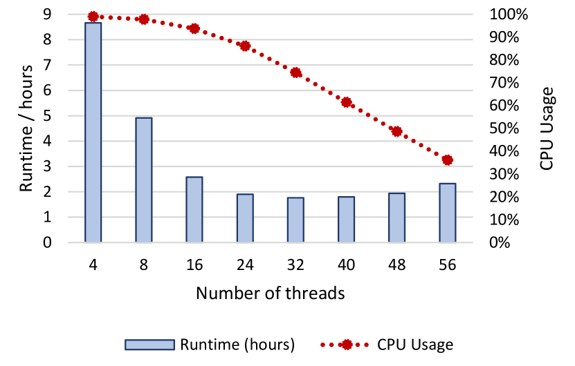
Figure H.1: Variation of runtime of original Nanopolish with the number of threads

To verify the above mentioned limitation of the HDF5 library, we manually split the dataset into 14 roughly equal parts and then separately (but in parallel) launched 14 Nanopolish processes. Each process was launched with 4 threads, thus the 56 threads are expected to be active to be able to fully utilise all 56 cores. This 4 thread and 14 process configuration was selected since at 4 threads the CPU utilisation was around $\sim$100% (Fig. H.1). Since each process has its own address space and a synchronisation primitives in one process does not affect the other processes. How the CPU utilisation (calculated as in equation 7.1 out of all 56 CPU threads) varied with the time is in Fig. H.2.

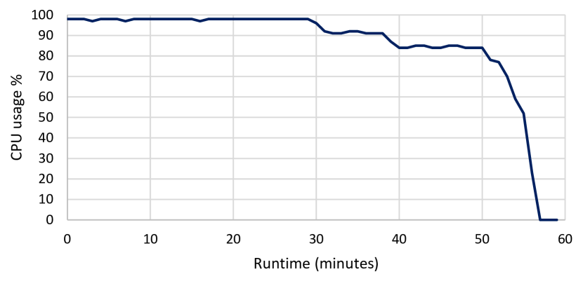
Figure H.2: CPU utilisation with the runtime

Observe that the CPU utilisation is closer to 100% up to around 30 minutes. After 30 minutes the drop in CPU utilisation is due to certain processors finishing earlier than the others. Nevertheless, this plot shows that the underlying disk system could service faster than the CPU could process and confirms that the low CPU utilisation when running one Nanopolish process with 56 threads was due to the limitation of underlying software (HDF5 library in this case).

H.2 Extended Deeper analysis of the Bottleneck using Another Dataset

We restructured Nanopolish such that time spent on I/O and processing can be separately measured. It is such that a batch of reads (several thousand) are read from the disk using a single thread (to mimic the behaviours of the lock in HDF5) and the batch is assigned to multiple threads equal to the maximum number of cores to be processed. This repeats until all reads are processed. On system S1 (Table 7.4) for the dataset D2 (Table H.1), the execution time was 72.19 hours (3 days!). Data loading ridiculously contributed took 95.96% of the total time (69.27) and only 4.04% for processing (2.92 h). Out of the time for data loading, reading of FAST5 files (HDF5) ridiculously contributed to 90.54% (62.72h). Random access to FASTQ/FASTA files performed using faidx in htslib took 8.58% (5.95) and sequential access to the BAM file performed through htslib took only 0.88% (0.58h).

Instead of a single thread performing FAST5 reading, now we ran the experiment with multiple threads to further consolidate our explanation of the HDF5 bottleneck. Dataset D1 (manageable runtime than D2 for extensive testing) was used and the experiment was conducted on two systems, S1 that contains an HDD RAID and S2 with an SSD RAID (refer to Tables 7.4, 7.3 and H.1 for detailed information of the systems and the datasets). As expected, the time for reading FAST5 did not improve with the number of I/O threads as shown in the Fig. H.3. On the system with SSD RAID FAST5 access time even got worse with multiple threads. Similar to the dataset D2 above, processing time (performed using all available cores), FASTA access and BAM access (performed using 1 thread) took significantly lower time compared to FAST5 access for D1 as exemplified in Fig. H.3.

(a) on system S1 comprising HDD RAID

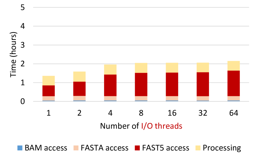
(b) on system S2 comprising SSD RAID

Figure H.3: Inefficiency of multi-threaded I/O to the HDF5 library

H.3 Extended Results

Table H.1: Dataset D2. D2 is an Oxford Nanopore PromethION dataset. D2 was only used for a limited number of experiments due to the massive execution time (up to 72 hours).

ID	Sample	No. of Gbases	No. of reads	average read length	max read length	FASTQ file size	FAST5 file size
D2	NA12878	66.093	23 654 340	2794.13	1 034 523	127GB	1.6TB

Table H.2: System used for experiment in section H.1

ID	Description	CPU	CPU cores	RAM	Disk System	RAID configuration	OS
S4	server with SSD RAID array	Intel Xeon CPU E5-2680	28	512 GB	10 NVMe drives	RAID10	Centos 7

H.3.1 Results from Alternate File Format (SLOW5) for Another Dataset

For the large D2 dataset we ran with all cores available on server S1 and the overall execution time improved to 22.04 hours for restructured Nanopolish with SLOW5 which was 69.29 hours previously for FAST (mentioned in section H.2). The FAST5 access time which was around 62 hours earlier (mentioned in section H.2) improved to around 6 hours when our SLOW5 format was used.

H.3.2 Impact of Proposed Solutions on Disk IOPS

System resource utilisation statistics for original Nanopolish, optimised Nanopolish with SLOW5 format and optimised Nanopolish with FAST5 multi-process pool are in Fig. H.4, Fig. H.5 and Fig. H.6, respectively. The statistics were collected using the collectl utility in Linux while each application was executing with 32 threads on System S1.

Observe that disk Input/output operations per second (IOPS) for SLOW5 format is lesser than that for the FAST5 multi-process pool while the disk I/O (amount of data read per second) for SLOW5 format is larger than for the FAST5 multi-process pool. This observation demonstrates the efficacy of SLOW5 format that exploits the locality in data for efficient disk access. Storing all the data and metadata associated with a genomic-read in a single contiguous record reduces the random disk access operations (IOPS) while increasing the amount of data read per second.

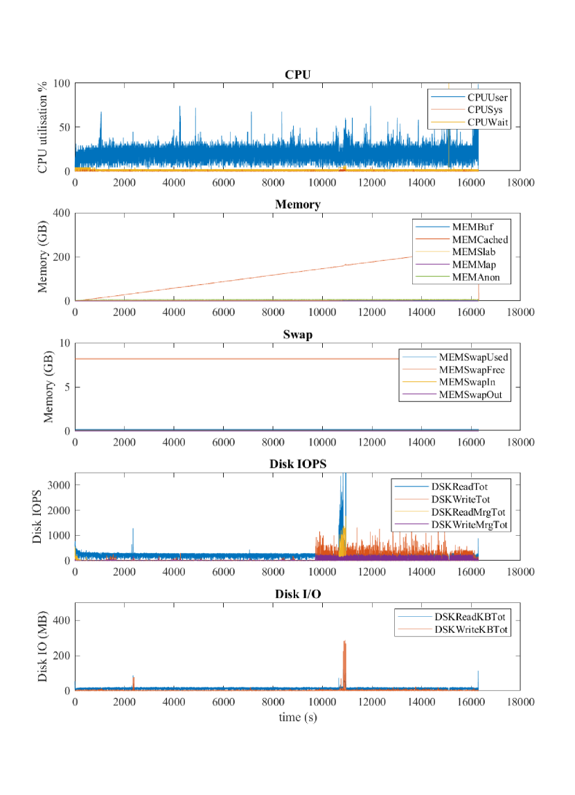
Figure H.4: Statistics collected using collectl for Nanopolish

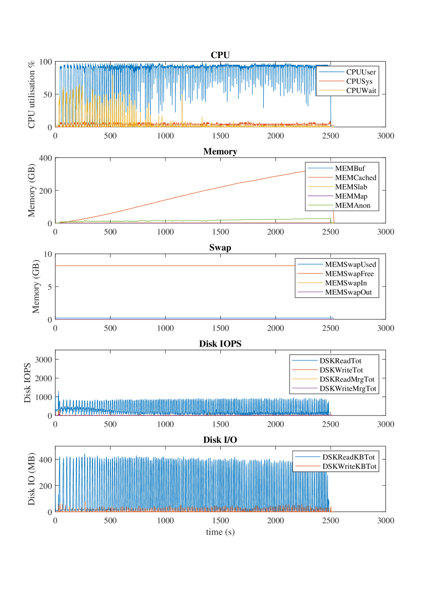
Figure H.5: Statistics collected using collectl for SLOW5

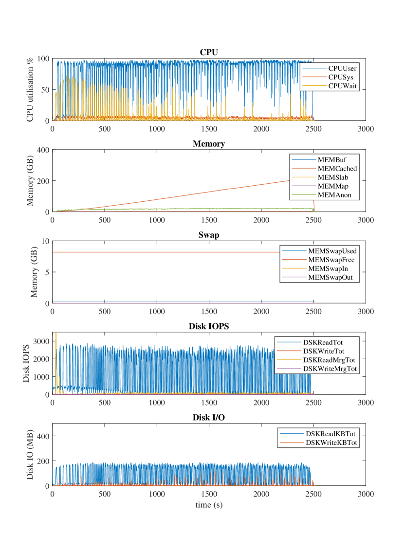
Figure H.6: Statistics collected using collectl for FAST5 multi-process pool

Appendix I Poster Presentations

The poster presented at Australasian Genomic Technologies Association (AGTA) Conference 2019 that attracted the best student poster award is in Fig. I.1

The poster presented at ACM SRC at ESWEEK 2019 that was shortlisted to the next level in the competition is in Fig. I.2

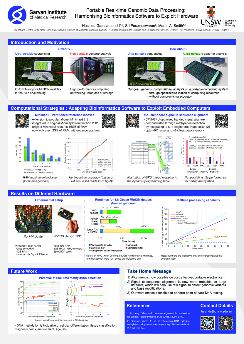
Figure I.1: Poster presented at AGTA 2019

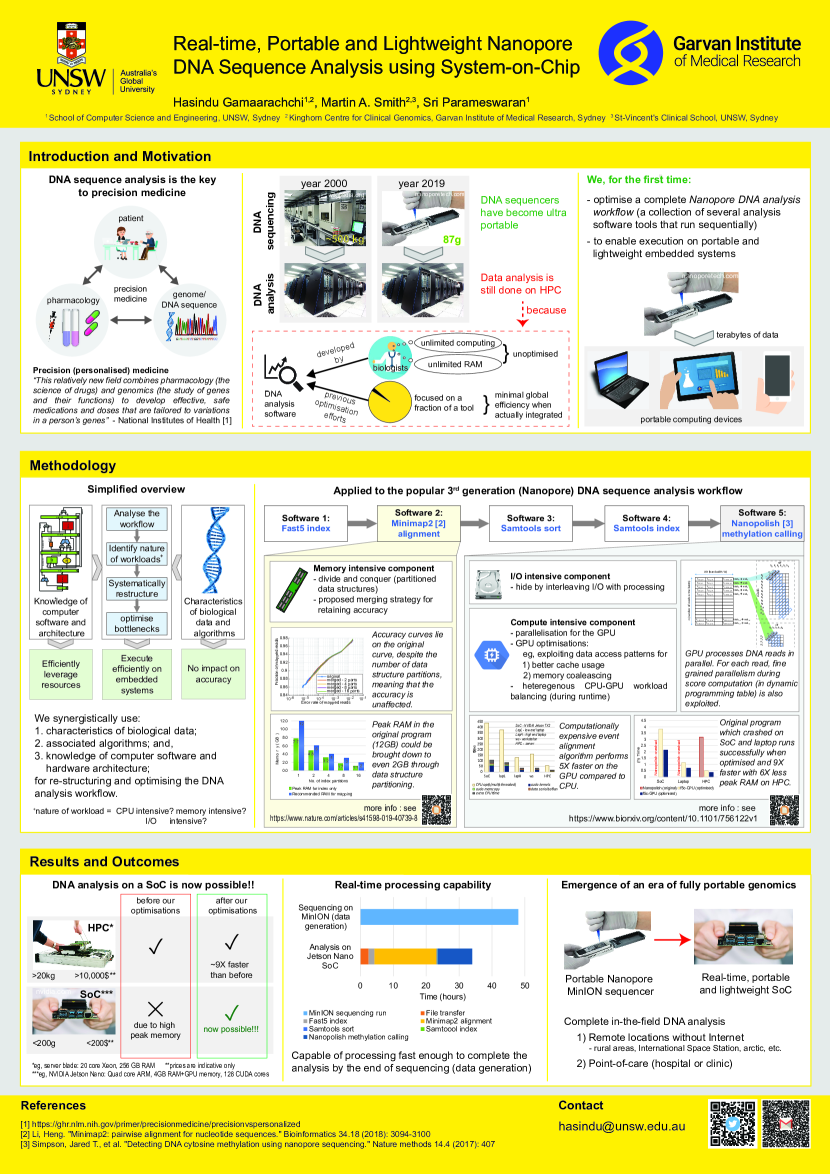
Figure I.2: Poster presented at ACM SRC at ESWEEK 2019

References

- [1] H. Chial, “DNA sequencing technologies key to the Human Genome Project,” Nature Education, vol. 1, no. 1, p. 219, 2008.
- [2] NIH, “The human genome project completion: Frequently asked questions,” 2010, Accessed: Jul 28, 2020. [Online]. Available: https://www.genome.gov/11006943/human-genome-project-completion-frequently-asked-questions
- [3] Garvan Institute, “The future of genomic medicine has arrived in Australia,” 2014, Accessed: Jul 28, 2020. [Online]. Available: {https://www.garvan.org.au/news-events/news/the-future-of-genomic-medicine-has-arrived-in-australia}
- [4] B. J. Fikes, “New machines can sequence human genome in one hour, Illumina announces,” 2017, Accessed: Jul 28, 2020. [Online]. Available: http://www.sandiegouniontribune.com/business/biotech/sd-me-illumina-novaseq-20170109-story.html
- [5] Illumina, “Illumina Introduces the NovaSeq Series - a New Architecture Designed to Usher in the 100$ Genome,” 2017, Accessed: Jul 28, 2020. [Online]. Available: {https://sapac.illumina.com/company/news-center/press-releases/2017/2236383.html}
- [6] National Institutes of Health, “Precision medicine,” 2020, Accessed: Jul 30, 2020. [Online]. Available: https://ghr.nlm.nih.gov/primer/precisionmedicine.pdf
- [7] E. A. Ashley, “Towards precision medicine,” Nature Reviews Genetics, vol. 17, no. 9, p. 507, 2016.
- [8] N. J. Schork, “Personalized medicine: time for one-person trials,” Nature, vol. 520, no. 7549, pp. 609–611, 2015.
- [9] G. S. Ginsburg and J. J. McCarthy, “Personalized medicine: revolutionizing drug discovery and patient care,” TRENDS in Biotechnology, vol. 19, no. 12, pp. 491–496, 2001.
- [10] A. T. Shaw, B. Solomon, and M. M. Kenudson, “Crizotinib and testing for ALK,” Journal of the National Comprehensive Cancer Network, vol. 9, no. 12, pp. 1335–1341, 2011.
- [11] B. Souffreau, “The human genome,” Jan 2009, Accessed: Jul 28, 2020. [Online]. Available: https://www.flickr.com/photos/bram_souffreau/3199664383
- [12] S. Levy, G. Sutton, P. C. Ng, L. Feuk, A. L. Halpern, B. P. Walenz, N. Axelrod, J. Huang, E. F. Kirkness, G. Denisov et al., “The diploid genome sequence of an individual human,” PLoS biology, vol. 5, no. 10, p. e254, 2007.
- [13] A. J. de Koning, W. Gu, T. A. Castoe, M. A. Batzer, and D. D. Pollock, “Repetitive elements may comprise over two-thirds of the human genome,” PLoS Genet, vol. 7, no. 12, p. e1002384, 2011.
- [14] T. J. Treangen and S. L. Salzberg, “Repetitive DNA and next-generation sequencing: computational challenges and solutions,” Nature Reviews Genetics, vol. 13, no. 1, pp. 36–46, 2012.
- [15] K. A. Wetterstrand, “Dna sequencing costs: Data from the nhgri genome sequencing program (gsp),” 2019, Accessed: Jul 28, 2020. [Online]. Available: https://www.genome.gov/about-genomics/fact-sheets/DNA-Sequencing-Costs-Data
- [16] J. Quick, N. J. Loman, S. Duraffour, J. T. Simpson, E. Severi, L. Cowley, J. A. Bore, R. Koundouno, G. Dudas, A. Mikhail, and others, “Real-time, portable genome sequencing for Ebola surveillance,” Nature, vol. 530, no. 7589, p. 228, 2016.
- [17] N. R. Faria, E. C. Sabino, M. R. T. Nunes, L. C. J. Alcantara, N. J. Loman, and O. G. Pybus, “Mobile real-time surveillance of Zika virus in Brazil,” Genome Medicine, vol. 8, no. 1, p. 97, 9 2016. [Online]. Available: https://doi.org/10.1186/s13073-016-0356-2
- [18] J. Goordial, I. Altshuler, K. Hindson, K. Chan-Yam, E. Marcolefas, and L. G. Whyte, “In situ field sequencing and life detection in remote (79 26’ N) Canadian high arctic permafrost ice wedge microbial communities,” Frontiers in microbiology, vol. 8, p. 2594, 2017.
- [19] S. L. Castro-Wallace, C. Y. Chiu, K. K. John, S. E. Stahl, K. H. Rubins, A. B. R. McIntyre, J. P. Dworkin, M. L. Lupisella, D. J. Smith, D. J. Botkin, and others, “Nanopore DNA sequencing and genome assembly on the International Space Station,” Scientific reports, vol. 7, no. 1, p. 18022, 2017.
- [20] NanoporeTech, “Novel Coronavirus (COVID-19) Overview,” 2020, Accessed: Jul 28, 2020. [Online]. Available: https://nanoporetech.com/covid-19/overview
- [21] J. L. Hennessy and D. A. Patterson, “A new golden age for computer architecture: Domain-specific hardware/software co-design, enhanced security, open instruction sets, and agile chip development,” Turing Lecture, 2018.
- [22] J. Jurka, W. Bao, K. Kojima, and V. V. Kapitonov, “Repetitive elements: bioinformatic identification, classification and analysis,” eLS, 2011.
- [23] K. H. Miga, S. Koren, A. Rhie, M. R. Vollger, A. Gershman, A. Bzikadze, S. Brooks, E. Howe, D. Porubsky, G. A. Logsdon et al., “Telomere-to-telomere assembly of a complete human x chromosome,” BioRxiv, p. 735928, 2019.
- [24] H. Gamaarachchi, A. Bayat, B. Gaeta, and S. Parameswaran, “Cache Friendly Optimisation of de Bruijn Graph based Local Re-assembly in Variant Calling,” IEEE/ACM transactions on computational biology and bioinformatics, 2018.
- [25] H. Gamaarachchi, S. Parameswaran, and M. A. Smith, “Featherweight long read alignment using partitioned reference indexes,” Scientific Reports, vol. 9, no. 1, p. 4318, 2019.
- [26] H. Gamaarachchi, C. W. Lam, G. Jayatilaka, H. Samarakoon, J. T. Simpson, M. A. Smith, and S. Parameswaran, “GPU Accelerated Adaptive Banded Event Alignment for Rapid Comparative Nanopore Signal Analysis,” bioRxiv, 2019.
- [27] R. P. Mohanty, H. Gamaarachchi, A. Lambert, and S. Parameswaran, “SWARAM: Portable Energy and Cost Efficient Embedded System for Genomic Processing,” ACM Transactions on Embedded Computing Systems (TECS), vol. 18, no. 5s, pp. 1–24, 2019.
- [28] H. Samarakoon, S. Punchihewa, A. Senanayake, R. Ragel, and H. Gamaarachchi, “F5N: Nanopore Sequence Analysis Toolkit for Android Smartphones,” bioRxiv, 2020.
- [29] A. Bayat, H. Gamaarachchi, N. P. Deshpande, M. R. Wilkins, and S. Parameswaran, “Methods for de-novo genome assembly,” Preprints 2020, 2020.
- [30] G. Felsenfeld, “DNA.” Scientific American, vol. 253, no. 4, pp. 58–67, 1985.
- [31] Ensembl, “Repeats,” 2020, Accessed: Jul 28, 2020. [Online]. Available: https://asia.ensembl.org/info/genome/genebuild/assembly_repeats.html
- [32] A. S. Kondrashov and I. B. Rogozin, “Context of deletions and insertions in human coding sequences,” Human mutation, vol. 23, no. 2, pp. 177–185, 2004.
- [33] M. Mahmoud, N. Gobet, D. I. Cruz-Dávalos, N. Mounier, C. Dessimoz, and F. J. Sedlazeck, “Structural variant calling: the long and the short of it,” Genome biology, vol. 20, no. 1, p. 246, 2019.
- [34] V. Ingram, “A specific chemical difference between the globins of normal human and sickle cell anemia hemoglobin,” Nature, vol. 178, no. Oct 13, pp. 792–794, 1956.
- [35] J. C. Chang and Y. W. Kan, “beta 0 thalassemia, a nonsense mutation in man,” Proceedings of the National Academy of Sciences, vol. 76, no. 6, pp. 2886–2889, 1979.
- [36] C. Ober and T.-C. Yao, “The genetics of asthma and allergic disease: a 21st century perspective,” Immunological reviews, vol. 242, no. 1, pp. 10–30, 2011.
- [37] M. J. Landrum, J. M. Lee, G. R. Riley, W. Jang, W. S. Rubinstein, D. M. Church, and D. R. Maglott, “Clinvar: public archive of relationships among sequence variation and human phenotype,” Nucleic acids research, vol. 42, no. D1, pp. D980–D985, 2013.
- [38] Samtools organisation, “The Variant Call Format (VCF) Version 4.2 Specification,” 2020, Accessed: Jul 28, 2020. [Online]. Available: https://samtools.github.io/hts-specs/VCFv4.2.pdf
- [39] L. Xu and M. Seki, “Recent advances in the detection of base modifications using the nanopore sequencer,” Journal of human genetics, pp. 1–9, 2019.
- [40] J. M. Heather and B. Chain, “The sequence of sequencers: the history of sequencing dna,” Genomics, vol. 107, no. 1, pp. 1–8, 2016.
- [41] P. J. Cock, C. J. Fields, N. Goto, M. L. Heuer, and P. M. Rice, “The Sanger FASTQ file format for sequences with quality scores, and the Solexa/Illumina FASTQ variants,” Nucleic acids research, vol. 38, no. 6, pp. 1767–1771, 2009.
- [42] B. Ewing and P. Green, “Base-calling of automated sequencer traces using phred. ii. error probabilities,” Genome research, vol. 8, no. 3, pp. 186–194, 1998.
- [43] F. Sanger, G. M. Air, B. G. Barrell, N. L. Brown, A. R. Coulson, J. C. Fiddes, C. Hutchison, P. M. Slocombe, and M. Smith, “Nucleotide sequence of bacteriophage X174 DNA,” nature, vol. 265, no. 5596, pp. 687–695, 1977.
- [44] F. Sanger, S. Nicklen, and A. R. Coulson, “DNA sequencing with chain-terminating inhibitors,” Proceedings of the national academy of sciences, vol. 74, no. 12, pp. 5463–5467, 1977.
- [45] L. Liu, Y. Li, S. Li, N. Hu, Y. He, R. Pong, D. Lin, L. Lu, and M. Law, “Comparison of next-generation sequencing systems,” BioMed research international, vol. 2012, 2012.
- [46] J. C. Venter, M. D. Adams, E. W. Myers, P. W. Li, R. J. Mural, G. G. Sutton, H. O. Smith, M. Yandell, C. A. Evans, R. A. Holt et al., “The sequence of the human genome,” science, vol. 291, no. 5507, pp. 1304–1351, 2001.
- [47] S. Jurvetson, “Riding shotgun,” 2005, Accessed: Jul 28, 2020. [Online]. Available: https://www.flickr.com/photos/jurvetson/57080968
- [48] Applied Biosystems, “3730xl DNA Analyzer,” Accessed: Jul 28, 2020. [Online]. Available: https://www.thermofisher.com/order/catalog/product/3730XL#/3730XL
- [49] P. Nyrén and A. Lundin, “Enzymatic method for continuous monitoring of inorganic pyrophosphate synthesis,” Analytical biochemistry, vol. 151, no. 2, pp. 504–509, 1985.
- [50] HiSeqX Series of Sequencing Systems, Illumina, 2016.
- [51] D. I. Lou, J. A. Hussmann, R. M. McBee, A. Acevedo, R. Andino, W. H. Press, and S. L. Sawyer, “High-throughput dna sequencing errors are reduced by orders of magnitude using circle sequencing,” Proceedings of the National Academy of Sciences, vol. 110, no. 49, pp. 19 872–19 877, 2013.
- [52] E. C. Hayden, “Genome sequencing: the third generation,” Nature, vol. 457, no. 7231, pp. 768–9, 2009.
- [53] E. E. Schadt, S. Turner, and A. Kasarskis, “A window into third-generation sequencing,” Human molecular genetics, vol. 19, no. R2, pp. R227–R240, 2010.
- [54] Z.-G. Wei and S.-W. Zhang, “NPBSS: a new PacBio sequencing simulator for generating the continuous long reads with an empirical model,” BMC bioinformatics, vol. 19, no. 1, p. 177, 2018.
- [55] R. R. Wick, L. M. Judd, and K. E. Holt, “Performance of neural network basecalling tools for oxford nanopore sequencing,” Genome biology, vol. 20, no. 1, p. 129, 2019.
- [56] M. Jain, S. Koren, K. H. Miga, J. Quick, A. C. Rand, T. A. Sasani, J. R. Tyson, A. D. Beggs, A. T. Dilthey, I. T. Fiddes, and others, “Nanopore sequencing and assembly of a human genome with ultra-long reads,” Nature biotechnology, vol. 36, no. 4, p. 338, 2018.
- [57] H. Li, B. Handsaker, A. Wysoker, T. Fennell, J. Ruan, N. Homer, G. Marth, G. Abecasis, and R. Durbin, “The sequence alignment/map format and SAMtools,” Bioinformatics, vol. 25, no. 16, pp. 2078–2079, 2009.
- [58] Broad Institute, “Picard,” 2018, Accessed: Jul 28, 2020. [Online]. Available: http://broadinstitute.github.io/picard/
- [59] A. Tarasov, A. J. Vilella, E. Cuppen, I. J. Nijman, and P. Prins, “Sambamba: fast processing of NGS alignment formats,” Bioinformatics, vol. 31, no. 12, pp. 2032–2034, 2015.
- [60] D. Sims, I. Sudbery, N. E. Ilott, A. Heger, and C. P. Ponting, “Sequencing depth and coverage: key considerations in genomic analyses,” Nature Reviews Genetics, vol. 15, no. 2, pp. 121–132, 2014.
- [61] S.-M. Ahn, T.-H. Kim, S. Lee, D. Kim, H. Ghang, D.-S. Kim, B.-C. Kim, S.-Y. Kim, W.-Y. Kim, C. Kim et al., “The first korean genome sequence and analysis: full genome sequencing for a socio-ethnic group,” Genome research, vol. 19, no. 9, pp. 1622–1629, 2009.
- [62] P. Flicek and E. Birney, “Sense from sequence reads: methods for alignment and assembly,” Nature methods, vol. 6, pp. S6–S12, 2009.
- [63] M. Burrows and D. J. Wheeler, “A block-sorting lossless data compression algorithm,” Digital SRC Research Report, 1994.
- [64] H. Li, J. Ruan, and R. Durbin, “Mapping short DNA sequencing reads and calling variants using mapping quality scores,” Genome research, vol. 18, no. 11, pp. 1851–1858, 2008.
- [65] R. Li, Y. Li, K. Kristiansen, and J. Wang, “SOAP: short oligonucleotide alignment program,” Bioinformatics, vol. 24, no. 5, pp. 713–714, 2008.
- [66] N. Homer, B. Merriman, and S. F. Nelson, “BFAST: an alignment tool for large scale genome resequencing,” PloS one, vol. 4, no. 11, p. e7767, 2009.
- [67] P. Ferragina and G. Manzini, “Opportunistic data structures with applications,” in Foundations of Computer Science, 2000. Proceedings. 41st Annual Symposium on. IEEE, 2000, pp. 390–398.
- [68] B. Langmead, C. Trapnell, M. Pop, and S. L. Salzberg, “Ultrafast and memory-efficient alignment of short DNA sequences to the human genome,” Genome biology, vol. 10, no. 3, p. R25, 2009.
- [69] B. Langmead and S. L. Salzberg, “Fast gapped-read alignment with bowtie 2,” Nature methods, vol. 9, no. 4, p. 357, 2012.
- [70] H. Li and R. Durbin, “Fast and accurate short read alignment with Burrows–Wheeler transform,” Bioinformatics, vol. 25, no. 14, pp. 1754–1760, 2009.
- [71] ——, “Fast and accurate long-read alignment with Burrows–Wheeler transform,” Bioinformatics, vol. 26, no. 5, pp. 589–595, 2010.
- [72] H. Li, “Aligning sequence reads, clone sequences and assembly contigs with BWA-MEM,” arXiv preprint arXiv:1303.3997, 2013.
- [73] R. Li, C. Yu, Y. Li, T.-W. Lam, S.-M. Yiu, K. Kristiansen, and J. Wang, “SOAP2: an improved ultrafast tool for short read alignment,” Bioinformatics, vol. 25, no. 15, pp. 1966–1967, 2009.
- [74] S. B. Needleman and C. D. Wunsch, “A general method applicable to the search for similarities in the amino acid sequence of two proteins,” Journal of molecular biology, vol. 48, no. 3, pp. 443–453, 1970.
- [75] T. F. Smith and M. S. Waterman, “Identification of common molecular subsequences,” Journal of molecular biology, vol. 147, no. 1, pp. 195–197, 1981.
- [76] R. Durbin, S. R. Eddy, A. Krogh, and G. Mitchison, Biological sequence analysis: probabilistic models of proteins and nucleic acids. Cambridge university press, 1998.
- [77] K.-M. Chao, W. R. Pearson, and W. Miller, “Aligning two sequences within a specified diagonal band,” Bioinformatics, vol. 8, no. 5, pp. 481–487, 1992.
- [78] S. F. Altschul, T. L. Madden, A. A. Schäffer, J. Zhang, Z. Zhang, W. Miller, and D. J. Lipman, “Gapped BLAST and PSI-BLAST: a new generation of protein database search programs,” Nucleic acids research, vol. 25, no. 17, pp. 3389–3402, 1997.
- [79] S. Sandmann, A. O. De Graaf, M. Karimi, B. A. Van Der Reijden, E. Hellström-Lindberg, J. H. Jansen, and M. Dugas, “Evaluating variant calling tools for non-matched next-generation sequencing data,” Scientific Reports, vol. 7, p. 43169, 2017.
- [80] M. A. DePristo, E. Banks, R. Poplin, K. V. Garimella, J. R. Maguire, C. Hartl, A. A. Philippakis, G. Del Angel, M. A. Rivas, M. Hanna et al., “A framework for variation discovery and genotyping using next-generation DNA sequencing data,” Nature genetics, vol. 43, no. 5, pp. 491–498, 2011.
- [81] R. Poplin, V. Ruano-Rubio, M. A. DePristo, T. J. Fennell, M. O. Carneiro, G. A. Van der Auwera, D. E. Kling, L. D. Gauthier, A. Levy-Moonshine, D. Roazen et al., “Scaling accurate genetic variant discovery to tens of thousands of samples,” BioRxiv, p. 201178, 2018.
- [82] E. Garrison and G. Marth, “Haplotype-based variant detection from short-read sequencing,” arXiv preprint arXiv:1207.3907, 2012.
- [83] H. Li, “A statistical framework for SNP calling, mutation discovery, association mapping and population genetical parameter estimation from sequencing data,” Bioinformatics, vol. 27, no. 21, pp. 2987–2993, 2011.
- [84] A. Rimmer, H. Phan, I. Mathieson, Z. Iqbal, S. R. Twigg, A. O. Wilkie, G. McVean, G. Lunter, W. Consortium et al., “Integrating mapping-, assembly-and haplotype-based approaches for calling variants in clinical sequencing applications,” Nature genetics, vol. 46, no. 8, pp. 912–918, 2014.
- [85] Z. Wei, W. Wang, P. Hu, G. J. Lyon, and H. Hakonarson, “SNVer: a statistical tool for variant calling in analysis of pooled or individual next-generation sequencing data,” Nucleic acids research, vol. 39, no. 19, pp. e132–e132, 2011.
- [86] D. C. Koboldt, Q. Zhang, D. E. Larson, D. Shen, M. D. McLellan, L. Lin, C. A. Miller, E. R. Mardis, L. Ding, and R. K. Wilson, “VarScan 2: somatic mutation and copy number alteration discovery in cancer by exome sequencing,” Genome research, vol. 22, no. 3, pp. 568–576, 2012.
- [87] C. Alkan, B. P. Coe, and E. E. Eichler, “Genome structural variation discovery and genotyping,” Nature reviews. Genetics, vol. 12, no. 5, p. 363, 2011.
- [88] N. Homer and S. F. Nelson, “Improved variant discovery through local re-alignment of short-read next-generation sequencing data using SRMA,” Genome biology, vol. 11, no. 10, p. R99, 2010.
- [89] Z. Iqbal, M. Caccamo, I. Turner, P. Flicek, and G. McVean, “De novo assembly and genotyping of variants using colored de Bruijn graphs,” Nature Genetics, vol. 44, no. 2, pp. 226–232, 2012. [Online]. Available: http://dx.doi.org/10.1038/ng.1028
- [90] G. VdAuwera, “Hc overview: How the haplotypecaller works,” 2014, Accessed: July 8, 2017. [Online]. Available: https://gatkforums.broadinstitute.org/gatk/discussion/4148/hc-overview-how-the-haplotypecaller-works
- [91] L. Pachter, M. Alexandersson, and S. Cawley, “Applications of generalized pair hidden markov models to alignment and gene finding problems,” Journal of Computational Biology, vol. 9, no. 2, pp. 389–399, 2002.
- [92] 1000 Genomes Project Consortium and others, “A map of human genome variation from population scale sequencing,” Nature, vol. 467, no. 7319, p. 1061, 2010.
- [93] Z. Lai, A. Markovets, M. Ahdesmaki, B. Chapman, O. Hofmann, R. McEwen, J. Johnson, B. Dougherty, J. C. Barrett, and J. R. Dry, “VarDict: a novel and versatile variant caller for next-generation sequencing in cancer research,” Nucleic acids research, vol. 44, no. 11, pp. e108–e108, 2016.
- [94] Broad Institute, “Haplotypecaller,” 2020, Accessed: Jul 28, 2020. [Online]. Available: https://gatk.broadinstitute.org/hc/en-us/articles/360037225632-HaplotypeCaller
- [95] HDF Group, “HDF5 Specifications,” 2014, Accessed: Jul 28, 2020. [Online]. Available: https://support.hdfgroup.org/HDF5/doc/Specs.html
- [96] M. J. Chaisson and G. Tesler, “Mapping single molecule sequencing reads using basic local alignment with successive refinement (BLASR): application and theory,” BMC bioinformatics, vol. 13, no. 1, p. 238, 2012.
- [97] I. Sović, M. Šikić, A. Wilm, S. N. Fenlon, S. Chen, and N. Nagarajan, “Fast and sensitive mapping of nanopore sequencing reads with GraphMap,” Nature communications, vol. 7, p. 11307, 2016.
- [98] H.-N. Lin and W.-L. Hsu, “Kart: a divide-and-conquer algorithm for NGS read alignment,” Bioinformatics, vol. 33, no. 15, pp. 2281–2287, 2017.
- [99] F. J. Sedlazeck, P. Rescheneder, M. Smolka, H. Fang, M. Nattestad, A. von Haeseler, and M. C. Schatz, “Accurate detection of complex structural variations using single-molecule sequencing,” Nature Methods, vol. 15, no. 6, pp. 461–468, 2018. [Online]. Available: https://doi.org/10.1038/s41592-018-0001-7
- [100] B. Liu, Y. Gao, and Y. Wang, “LAMSA: fast split read alignment with long approximate matches,” Bioinformatics, vol. 33, no. 2, pp. 192–201, 2017.
- [101] H. Li, “Minimap2: pairwise alignment for nucleotide sequences,” Bioinformatics, p. bty191, 2018. [Online]. Available: http://dx.doi.org/10.1093/bioinformatics/bty191
- [102] H. Suzuki and M. Kasahara, “Introducing difference recurrence relations for faster semi-global alignment of long sequences,” BMC bioinformatics, vol. 19, no. 1, p. 45, 2018.
- [103] N. J. Loman, J. Quick, and J. T. Simpson, “A complete bacterial genome assembled de novo using only nanopore sequencing data,” Nature methods, vol. 12, no. 8, p. 733, 2015.
- [104] J. T. Simpson, R. E. Workman, P. Zuzarte, M. David, L. Dursi, and W. Timp, “Detecting DNA cytosine methylation using nanopore sequencing,” Nature methods, vol. 14, no. 4, p. 407, 2017.
- [105] NanoporeTech, “Medaka,” Accessed: Jul 28, 2020. [Online]. Available: https://github.com/nanoporetech/medaka
- [106] R. Luo, F. J. Sedlazeck, T.-W. Lam, and M. C. Schatz, “A multi-task convolutional deep neural network for variant calling in single molecule sequencing,” Nature communications, vol. 10, no. 1, pp. 1–11, 2019.
- [107] R. Luo, C.-L. Wong, Y.-S. Wong, C.-I. Tang, C.-M. Liu, C.-M. Leung, and T.-W. Lam, “Exploring the limit of using a deep neural network on pileup data for germline variant calling,” Nature Machine Intelligence, pp. 1–8, 2020.
- [108] H. Peltola, H. Söderlund, and E. Ukkonen, “SEQAID: A DNA sequence assembling program based on a mathematical model,” Nucleic Acids Research, 1984.
- [109] D. R. Zerbino and E. Birney, “Velvet: algorithms for de novo short read assembly using de bruijn graphs,” Genome research, vol. 18, no. 5, pp. 821–829, 2008.
- [110] J. T. Simpson, K. Wong, S. D. Jackman, J. E. Schein, S. J. Jones, and I. Birol, “ABySS: a parallel assembler for short read sequence data,” Genome research, vol. 19, no. 6, pp. 1117–1123, 2009.
- [111] A. Bankevich, S. Nurk, D. Antipov, A. A. Gurevich, M. Dvorkin, A. S. Kulikov, V. M. Lesin, S. I. Nikolenko, S. Pham, A. D. Prjibelski et al., “SPAdes: a new genome assembly algorithm and its applications to single-cell sequencing,” Journal of computational biology, vol. 19, no. 5, pp. 455–477, 2012.
- [112] Z. Iqbal, M. Caccamo, I. Turner, P. Flicek, and G. McVean, “De novo assembly and genotyping of variants using colored de bruijn graphs,” Nature genetics, vol. 44, no. 2, pp. 226–232, 2012.
- [113] J. T. Simpson and R. Durbin, “Efficient de novo assembly of large genomes using compressed data structures,” Genome research, vol. 22, no. 3, pp. 549–556, 2012.
- [114] E. W. Myers, “The fragment assembly string graph,” Bioinformatics, vol. 21, no. suppl_2, pp. ii79–ii85, 2005.
- [115] H. Li, “Minimap and miniasm: fast mapping and de novo assembly for noisy long sequences,” Bioinformatics, vol. 32, no. 14, pp. 2103–2110, 2016.
- [116] M. Kolmogorov, J. Yuan, Y. Lin, and P. A. Pevzner, “Assembly of long, error-prone reads using repeat graphs,” Nature biotechnology, vol. 37, no. 5, pp. 540–546, 2019.
- [117] S. Koren, B. P. Walenz, K. Berlin, J. R. Miller, N. H. Bergman, and A. M. Phillippy, “Canu: scalable and accurate long-read assembly via adaptive k-mer weighting and repeat separation,” Genome research, vol. 27, no. 5, pp. 722–736, 2017.
- [118] J. Ruan and H. Li, “Fast and accurate long-read assembly with wtdbg2,” Nature Methods, vol. 17, no. 2, pp. 155–158, 2020.
- [119] T. Rognes, “Faster smith-waterman database searches with inter-sequence simd parallelisation,” BMC bioinformatics, vol. 12, no. 1, p. 221, 2011.
- [120] J. Daily, “Parasail: SIMD C library for global, semi-global, and local pairwise sequence alignments,” BMC bioinformatics, vol. 17, no. 1, p. 81, 2016.
- [121] K. Reinert, T. H. Dadi, M. Ehrhardt, H. Hauswedell, S. Mehringer, R. Rahn, J. Kim, C. Pockrandt, J. Winkler, E. Siragusa et al., “The SeqAn C++ template library for efficient sequence analysis: A resource for programmers,” Journal of biotechnology, vol. 261, pp. 157–168, 2017.
- [122] M. Zhao, W.-P. Lee, E. P. Garrison, and G. T. Marth, “SSW library: an SIMD Smith-Waterman C/C++ library for use in genomic applications,” PloS one, vol. 8, no. 12, 2013.
- [123] A. Szalkowski, C. Ledergerber, P. Krähenbühl, and C. Dessimoz, “SWPS3–fast multi-threaded vectorized Smith-Waterman for IBM Cell/BE and 86/SSE2,” BMC research notes, vol. 1, no. 1, p. 107, 2008.
- [124] M. Vasimuddin, S. Misra, H. Li, and S. Aluru, “Efficient architecture-aware acceleration of BWA-MEM for multicore systems,” in 2019 IEEE International Parallel and Distributed Processing Symposium (IPDPS). IEEE, 2019, pp. 314–324.
- [125] S. S. Banerjee, A. P. Athreya, L. S. Mainzer, C. V. Jongeneel, W.-M. Hwu, Z. T. Kalbarczyk, and R. K. Iyer, “Efficient and scalable workflows for genomic analyses,” in Proceedings of the ACM International Workshop on Data-Intensive Distributed Computing, 2016, pp. 27–36.
- [126] M. Massie, F. Nothaft, C. Hartl, C. Kozanitis, A. Schumacher, A. D. Joseph, and D. A. Patterson, “ADAM: Genomics formats and processing patterns for cloud scale computing,” UCB/EECS-2013-207, EECS Department, University of California, Berkeley, Tech. Rep., 2013.
- [127] F. A. Nothaft, M. Massie, T. Danford, Z. Zhang, U. Laserson, C. Yeksigian, J. Kottalam, A. Ahuja, J. Hammerbacher, M. Linderman, M. Franklin, A. D. Joseph, and D. A. Patterson, “Rethinking data-intensive science using scalable analytics systems,” in Proceedings of the 2015 International Conference on Management of Data (SIGMOD ’15). ACM, 2015.
- [128] B. Langmead, M. C. Schatz, J. Lin, M. Pop, and S. L. Salzberg, “Searching for SNPs with cloud computing,” Genome biology, vol. 10, no. 11, p. R134, 2009.
- [129] M. C. Schatz, “CloudBurst: highly sensitive read mapping with mapreduce,” Bioinformatics, vol. 25, no. 11, pp. 1363–1369, 2009.
- [130] A. O’Driscoll, J. Daugelaite, and R. D. Sleator, “‘Big data’, Hadoop and cloud computing in genomics,” Journal of biomedical informatics, vol. 46, no. 5, pp. 774–781, 2013.
- [131] M. C. Schatz, B. Langmead, and S. L. Salzberg, “Cloud computing and the DNA data race,” Nature biotechnology, vol. 28, no. 7, pp. 691–693, 2010.
- [132] Y. Liu, W. Huang, J. Johnson, and S. Vaidya, “Gpu accelerated smith-waterman,” in International Conference on Computational Science. Springer, 2006, pp. 188–195.
- [133] S. A. Manavski and G. Valle, “CUDA compatible GPU cards as efficient hardware accelerators for Smith-Waterman sequence alignment,” BMC bioinformatics, vol. 9, no. 2, p. S10, 2008.
- [134] Y. Liu, D. L. Maskell, and B. Schmidt, “CUDASW++: optimizing Smith-Waterman sequence database searches for CUDA-enabled graphics processing units,” BMC Research Notes, vol. 2, no. 1, p. 73, 5 2009. [Online]. Available: http://bmcresnotes.biomedcentral.com/articles/10.1186/1756-0500-2-73
- [135] C.-M. Liu, T. Wong, E. Wu, R. Luo, S.-M. Yiu, Y. Li, B. Wang, C. Yu, X. Chu, K. Zhao et al., “SOAP3: ultra-fast GPU-based parallel alignment tool for short reads,” Bioinformatics, vol. 28, no. 6, pp. 878–879, 2012.
- [136] P. Klus, S. Lam, D. Lyberg, M. S. Cheung, G. Pullan, I. McFarlane, G. S. Yeo, and B. Y. Lam, “BarraCUDA - a fast short read sequence aligner using graphics processing units,” BMC research notes, vol. 5, no. 1, p. 27, 2012.
- [137] M. C. Schatz, C. Trapnell, A. L. Delcher, and A. Varshney, “High-throughput sequence alignment using graphics processing units,” BMC bioinformatics, vol. 8, no. 1, p. 474, 2007.
- [138] R. Luo, Y.-L. Wong, W.-C. Law, L.-K. Lee, J. Cheung, C.-M. Liu, and T.-W. Lam, “BALSA: integrated secondary analysis for whole-genome and whole-exome sequencing, accelerated by GPU,” PeerJ, vol. 2, p. e421, 2014.
- [139] Z. Feng, S. Qiu, L. Wang, and Q. Luo, “Accelerating long read alignment on three processors,” in Proceedings of the 48th International Conference on Parallel Processing. ACM, 2019, p. 71.
- [140] NVIDIA, “Clara genomics,” 2020, Accessed: Jan 06, 2020. [Online]. Available: https://developer.nvidia.com/Clara-Genomics
- [141] K. Benkrid, Y. Liu, and A. Benkrid, “A highly parameterized and efficient FPGA-based skeleton for pairwise biological sequence alignment,” IEEE Transactions on Very Large Scale Integration (VLSI) Systems, vol. 17, no. 4, pp. 561–570, 2009.
- [142] E. Houtgast, V.-M. Sima, and Z. Al-Ars, “High performance streaming Smith-Waterman implementation with implicit synchronization on intel FPGA using OpenCL,” in 2017 IEEE 17th International Conference on Bioinformatics and Bioengineering (BIBE). IEEE, 2017, pp. 492–496.
- [143] S. S. Banerjee, M. El-Hadedy, J. B. Lim, Z. T. Kalbarczyk, D. Chen, S. S. Lumetta, and R. K. Iyer, “Asap: Accelerated short-read alignment on programmable hardware,” IEEE Transactions on Computers, vol. 68, no. 3, pp. 331–346, 2018.
- [144] S. Huang, G. J. Manikandan, A. Ramachandran, K. Rupnow, W.-m. W. Hwu, and D. Chen, “Hardware Acceleration of the Pair-HMM Algorithm for DNA Variant Calling,” in Proceedings of the 2017 ACM/SIGDA International Symposium on Field-Programmable Gate Arrays. ACM, 2017, pp. 275–284.
- [145] S. S. Banerjee, M. El-Hadedy, C. Y. Tan, Z. T. Kalbarczyk, S. Lumetta, and R. K. Iyer, “On accelerating pair-HMM computations in programmable hardware,” in 2017 27th International Conference on Field Programmable Logic and Applications (FPL). IEEE, 2017, pp. 1–8.
- [146] Timelogic. (2017) DeCypher FPGA Biocomputing Systems. Accessed: Jul 28, 2020. [Online]. Available: http://www.timelogic.com/catalog/752/biocomputing-platforms
- [147] EdicoGenome, “The DRAGEN Engine,” 2017, Accessed: July 19, 2017. [Online]. Available: http://www.edicogenome.com/dragen-bioit-platform/the-dragen-engine-2/
- [148] ——, “Genome Pipeline,” 2017, Accessed: July 19, 2017. [Online]. Available: http://www.edicogenome.com/pipelines/dragen-genome-pipeline/
- [149] E. Rucci, C. Garcia, G. Botella, A. De Giusti, M. Naiouf, and M. Prieto-Matias, “SWIFOLD: Smith-Waterman implementation on FPGA with OpenCL for long DNA sequences,” BMC systems biology, vol. 12, no. 5, p. 96, 2018.
- [150] ——, “Accelerating smith-waterman alignment of long DNA sequences with OpenCL on FPGA,” in International Conference on Bioinformatics and Biomedical Engineering. Springer, 2017, pp. 500–511.
- [151] V. Gnanasambandapillai, A. Bayat, and S. Parameswaran, “Mesga: An mpsoc based embedded system solution for short read genome alignment,” in 2018 23rd Asia and South Pacific Design Automation Conference (ASP-DAC). IEEE, 2018, pp. 52–57.
- [152] Y. Turakhia, G. Bejerano, and W. J. Dally, “Darwin: A genomics co-processor provides up to 15,000x acceleration on long read assembly,” ACM SIGPLAN Notices, vol. 53, no. 2, pp. 199–213, 2018.
- [153] Reuters Events, “Celera’s paracel unit introduces genematcher 2,” 2001, Accessed: Jul 28, 2020. [Online]. Available: http://social.eyeforpharma.com/uncategorised/celeras-paracel-unit-introduces-genematcher-2
- [154] P. Muir, S. Li, S. Lou, D. Wang, D. J. Spakowicz, L. Salichos, J. Zhang, G. M. Weinstock, F. Isaacs, J. Rozowsky, and M. Gerstein, “The real cost of sequencing: scaling computation to keep pace with data generation,” Genome Biology, vol. 17, no. 1, p. 53, Mar 2016. [Online]. Available: https://doi.org/10.1186/s13059-016-0917-0
- [155] R. Nielsen, J. S. Paul, A. Albrechtsen, and Y. S. Song, “Genotype and SNP calling from next-generation sequencing data,” Nature Reviews Genetics, vol. 12, no. 6, pp. 443–451, 2011.
- [156] S. Li, R. Li, H. Li, J. Lu, Y. Li, L. Bolund, M. H. Schierup, and J. Wang, “SOAPindel: efficient identification of indels from short paired reads,” Genome research, vol. 23, no. 1, pp. 195–200, 2013.
- [157] G. Narzisi, J. A. O’rawe, I. Iossifov, H. Fang, Y.-h. Lee, Z. Wang, Y. Wu, G. J. Lyon, M. Wigler, and M. C. Schatz, “Accurate de novo and transmitted indel detection in exome-capture data using microassembly,” Nature methods, vol. 11, no. 10, pp. 1033–1036, 2014.
- [158] P. A. Pevzner, H. Tang, and M. S. Waterman, “An Eulerian path approach to DNA fragment assembly,” Proceedings of the National Academy of Sciences, vol. 98, no. 17, pp. 9748–9753, 2001.
- [159] H. Gamaarachchi, “Cache Optimised Platypus Variant Caller,” Accessed: Jul 28, 2020. [Online]. Available: https://github.com/hasindu2008/platycflr
- [160] C. Rauer and N. F. Jr, “Accelerating Genomics Research with OpenCL and FPGAs,” Altera Corporation, Tech. Rep. WP-01262-1.0, Mar. 2016.
- [161] G. VdAuwera, “Version highlights for GATK version 3.8,” 2017, Accessed: Jul 28, 2020. [Online]. Available: https://github.com/broadinstitute/gatk-docs/blob/master/blog-2012-to-2019/2017-07-29-Version_highlights_for_GATK_version_3.8.md?id=1006
- [162] F. Nothaft, “Scalable Genome Resequencing with ADAM and avocado,” Tech. Report No.: UCB/EECS-2015–65, 2015.
- [163] M. S. Hasan, X. Wu, and L. Zhang, “Performance evaluation of indel calling tools using real short-read data,” Human genomics, vol. 9, no. 1, p. 20, 2015.
- [164] R. Luo, B. Liu, Y. Xie, Z. Li, W. Huang, J. Yuan, G. He, Y. Chen, Q. Pan, Y. Liu et al., “SOAPdenovo2: an empirically improved memory-efficient short-read de novo assembler,” Gigascience, vol. 1, no. 1, p. 18, 2012.
- [165] R. Chikhi and G. Rizk, “Space-efficient and exact de bruijn graph representation based on a bloom filter,” Algorithms for Molecular Biology, vol. 8, no. 1, p. 22, 2013.
- [166] E. Georganas, A. Buluç, J. Chapman, L. Oliker, D. Rokhsar, and K. Yelick, “Parallel de bruijn graph construction and traversal for de novo genome assembly,” in Proceedings of the International Conference for High Performance Computing, Networking, Storage and Analysis. IEEE Press, 2014, pp. 437–448.
- [167] A. Rimmer, “Platypus Variant Caller,” Accessed: Jul 30, 2020. [Online]. Available: https://github.com/andyrimmer/Platypus
- [168] 1000genomes, “20120117_ceu_trio_b37_decoy,” 2012, Accessed: Jul 30, 2020. [Online]. Available: ftp://ftp.1000genomes.ebi.ac.uk/vol1/ftp/technical/working/20120117_ceu_trio_b37_decoy/
- [169] H. Mohamadi, B. P. Vandervalk, A. Raymond, S. D. Jackman, J. Chu, C. P. Breshears, and I. Birol, “DIDA: Distributed Indexing Dispatched Alignment,” PloS one, vol. 10, no. 4, p. e0126409, 2015.
- [170] T. H. Dadi, E. Siragusa, V. C. Piro, A. Andrusch, E. Seiler, B. Y. Renard, and K. Reinert, “DREAM-Yara: an exact read mapper for very large databases with short update time,” Bioinformatics, vol. 34, no. 17, pp. i766–i772, 2018. [Online]. Available: http://dx.doi.org/10.1093/bioinformatics/bty567
- [171] I. W. Deveson, W. Y. Chen, T. Wong, S. A. Hardwick, S. B. Andersen, L. K. Nielsen, J. S. Mattick, and T. R. Mercer, “Representing genetic variation with synthetic DNA standards,” Nature methods, vol. 13, no. 9, p. 784, 2016.
- [172] H. Li, “minimap,” 2015, Accessed: Jul 30, 2020. [Online]. Available: https://github.com/lh3/minimap/blob/master/README.md
- [173] D. W. Garsed, O. J. Marshall, V. D. Corbin, A. Hsu, L. Di Stefano, J. Schröder, J. Li, Z.-P. Feng, B. W. Kim, M. Kowarsky et al., “The architecture and evolution of cancer neochromosomes,” Cancer Cell, vol. 26, no. 5, pp. 653–667, 2014.
- [174] H. Li, H. Gamaarachchi, M. van den Beek, I. Kolpakov, J. Guo, martinghunt, …, and C. de Lannoy., “hasindu2008/minimap2-arm: long read alignment using partitioned reference indexes (version v0.1),” github http://doi.org/10.5281/zenodo.2011136, Dec 2018.
- [175] Y. Ono, K. Asai, and M. Hamada, “PBSIM: PacBio reads simulator—toward accurate genome assembly,” Bioinformatics, vol. 29, no. 1, pp. 119–121, 2012.
- [176] H. Li, “Paftools,” 2018, Accessed: Jul 30, 2020. [Online]. Available: https://github.com/lh3/minimap2/blob/master/misc/README.md
- [177] Y. Li, R. Han, C. Bi, M. Li, S. Wang, and X. Gao, “DeepSimulator: a deep simulator for Nanopore sequencing,” Bioinformatics, p. bty223, 2018. [Online]. Available: http://dx.doi.org/10.1093/bioinformatics/bty223
- [178] C. Yang, J. Chu, R. L. Warren, and I. Birol, “NanoSim: nanopore sequence read simulator based on statistical characterization,” GigaScience, vol. 6, no. 4, pp. 1–6, 2017.
- [179] P. C. Faucon, P. Balachandran, and S. Crook, “SNaReSim: Synthetic Nanopore Read Simulator,” in Healthcare Informatics (ICHI), 2017 IEEE International Conference on. IEEE, 2017, pp. 338–344.
- [180] AdamaJava, “Adamajava,” 2018, Accessed: Jul 30, 2020. [Online]. Available: https://github.com/AdamaJava/adamajava
- [181] A. R. Quinlan and I. M. Hall, “Bedtools: a flexible suite of utilities for comparing genomic features,” Bioinformatics, vol. 26, no. 6, pp. 841–842, 2010.
- [182] H. Gamaarachchi, S. Parasemwaran, and M. Smith, “Datasets and experiment data of long read alignment using partitioned reference indexes,” figshare https://doi.org/10.6084/m9.figshare.6964805.v1, Dec 2018.
- [183] V. Liyanage, J. Jarmasz, N. Murugeshan, M. Del Bigio, M. Rastegar, and J. Davie, “DNA modifications: function and applications in normal and disease states,” Biology, vol. 3, no. 4, pp. 670–723, 2014.
- [184] J. Lewandowska and A. Bartoszek, “Dna methylation in cancer development, diagnosis and therapy—multiple opportunities for genotoxic agents to act as methylome disruptors or remediators,” Mutagenesis, vol. 26, no. 4, pp. 475–487, 2011.
- [185] M. Fraser, V. Y. Sabelnykova, T. N. Yamaguchi, L. E. Heisler, J. Livingstone, V. Huang, Y.-J. Shiah, F. Yousif, X. Lin, A. P. Masella et al., “Genomic hallmarks of localized, non-indolent prostate cancer,” Nature, vol. 541, no. 7637, p. 359, 2017.
- [186] S. Saxonov, P. Berg, and D. L. Brutlag, “A genome-wide analysis of CpG dinucleotides in the human genome distinguishes two distinct classes of promoters,” Proceedings of the National Academy of Sciences, vol. 103, no. 5, pp. 1412–1417, 2006.
- [187] A. Bird, “DNA methylation patterns and epigenetic memory,” Genes & development, vol. 16, no. 1, pp. 6–21, 2002.
- [188] S. Gonzalo, “Epigenetic alterations in aging,” Journal of applied physiology, vol. 109, no. 2, pp. 586–597, 2010.
- [189] H. Lu, F. Giordano, and Z. Ning, “Oxford nanopore minion sequencing and genome assembly,” Genomics, proteomics & bioinformatics, vol. 14, no. 5, pp. 265–279, 2016.
- [190] F. J. Rang, W. P. Kloosterman, and J. de Ridder, “From squiggle to basepair: computational approaches for improving nanopore sequencing read accuracy,” Genome biology, vol. 19, no. 1, p. 90, 2018.
- [191] M. David, L. J. Dursi, D. Yao, P. C. Boutros, and J. T. Simpson, “Nanocall: an open source basecaller for oxford nanopore sequencing data,” Bioinformatics, vol. 33, no. 1, pp. 49–55, 2016.
- [192] NVIDIA, CUDA C Programming guide, September 2018, pG-02829-001_v10.0.
- [193] ——, CUDA C best practices guide, October 2018, dG-05603-001_v10.0.
- [194] Y. Liu, B. Schmidt, and D. L. Maskell, “CUDASW++2.0: enhanced Smith-Waterman protein database search on CUDA-enabled GPUs based on SIMT and virtualized SIMD abstractions,” BMC Research Notes, vol. 3, no. 1, p. 93, 4 2010. [Online]. Available: http://bmcresnotes.biomedcentral.com/articles/10.1186/1756-0500-3-93
- [195] Y. Liu, A. Wirawan, and B. Schmidt, “CUDASW++ 3.0: accelerating Smith-Waterman protein database search by coupling CPU and GPU SIMD instructions,” BMC Bioinformatics, vol. 14, no. 1, p. 117, 4 2013. [Online]. Available: http://bmcbioinformatics.biomedcentral.com/articles/10.1186/1471-2105-14-117
- [196] Oxford Nanopore Technologies, “MinIT is out - an analysis and device control accessory to enable powerful, real-time DNA/RNA sequencing by anyone, anywhere,” 2018, Accessed: Jul 30, 2020. [Online]. Available: https://nanoporetech.com/about-us/news/minit-launch
- [197] I. Huismann, M. Lieber, J. Stiller, and J. Fröhlich, “Load balancing for CPU-GPU coupling in computational fluid dynamics,” in International Conference on Parallel Processing and Applied Mathematics. Springer, 2017, pp. 337–347.
- [198] J. Lang and G. Rünger, “Dynamic distribution of workload between CPU and GPU for a parallel conjugate gradient method in an adaptive fem,” Procedia Computer Science, vol. 18, pp. 299–308, 2013.
- [199] Oxford Nanopore Technologies, “Ligation Sequencing Kit 1D or Rapid Sequencing Kit,” 2017, Accessed: Jul 30, 2020. [Online]. Available: https://store.nanoporetech.com/media/Ligation_Sequencing_Kit_1D_or_Rapid_Sequencing_Kit_v5_Feb2017.pdf
- [200] J. Simpson, “Stats and analysis,” 2017, Accessed: Jul 30, 2020. [Online]. Available: https://nanopolish.readthedocs.io/en/latest/quickstart_call_methylation.html
- [201] NVIDIA, Profiler user’s guide, March 2019, dU-05982-001_v10.1.
- [202] R. Chase, “How to configure the linux out-of-memory killer,” 2013, Accessed: Jul 30, 2020. [Online]. Available: https://www.oracle.com/technical-resources/articles/it-infrastructure/dev-oom-killer.html
- [203] Pine64, “ROCK64,” 2020, Accessed: Jul 30, 2020. [Online]. Available: https://wiki.pine64.org/index.php/ROCK64
- [204] F. Busatto, “TCP Keepalive HOWTO,” 2007, Accessed: Jul 30, 2020. [Online]. Available: http://tldp.org/HOWTO/TCP-Keepalive-HOWTO/programming.html
- [205] M. L. Massie, B. N. Chun, and D. E. Culler, “The ganglia distributed monitoring system: design, implementation, and experience,” Parallel Computing, vol. 30, no. 7, pp. 817–840, 2004.
- [206] Adiscon, “LogAnalyzer,” Accessed: Jul 30, 2020. [Online]. Available: https://loganalyzer.adiscon.com
- [207] M. Scholz, D. V. Ward, E. Pasolli, T. Tolio, M. Zolfo, F. Asnicar, D. T. Truong, A. Tett, A. L. Morrow, and N. Segata, “Strain-level microbial epidemiology and population genomics from shotgun metagenomics,” Nature methods, vol. 13, no. 5, pp. 435–438, 2016.
- [208] M. Riba, C. Sala, D. Toniolo, and G. Tonon, “Big data in medicine, the present and hopefully the future,” Frontiers in Medicine, vol. 6, 2019.
- [209] L. Schmitt, “From computational genomics to precision medicine,” 2016, Accessed: Jul 30, 2020. [Online]. Available: https://cs.illinois.edu/news/computational-genomics-precision-medicine
- [210] J. de Jesus, C. I. SC, F. Salles, E. Manulli, D. da Silva, T. de Paiva, M. Pinho, A. Afonso, A. Mathias, L. Prado et al., “First cases of coronavirus disease (covid-19) in brazil,” South America (2 genomes, 3rd March 2020)( http://virological. org/t/first-cases-ofcoronavirus-disease-covid-19-in-brazil-south-america-2-genomes-3rd-march-2020/409, Virological, 2020), 2020.
- [211] B. Schmidt and A. Hildebrandt, “Next-generation sequencing: big data meets high performance computing,” Drug discovery today, vol. 22, no. 4, pp. 712–717, 2017.
- [212] A. S. Bland, W. Joubert, D. E. Maxwell, N. Podhorszki, J. H. Rogers, and A. N. Tharrington, “Contemporary high performance computing from petascale toward exascale,” Oak Ridge National Lab.(ORNL), Oak Ridge, TN (United States); Center for …, Tech. Rep., 2013.
- [213] NanoporeTech, “Jared Simpson: Signal analysis using nanopolish,” 2019, Accessed: Jul 30, 2020. [Online]. Available: https://nanoporetech.com/resource-centre/jared-simpson-signal-analysis-using-nanopolish
- [214] K. Chan, “What are core-hours? how are they estimated?” 2019, Accessed: Jul 30, 2020. [Online]. Available: https://support.onscale.com/hc/en-us/articles/360013402431-What-are-Core-Hours-How-are-they-estimated-
- [215] J. Corbet, “Fixing asynchronous I/O, again,” Jan. 2016, Accessed: Jul 30, 2020. [Online]. Available: https://lwn.net/Articles/671649/
- [216] L. Torvalds, “Re: [PATCH 09/13] aio: add support for async openat(),” Jan. 2016, Accessed: Jul 30, 2020. [Online]. Available: https://lwn.net/Articles/671657/
- [217] M. Majkowski, “io_submit: The epoll alternative you’ve never heard about,” Jan. 2019, Accessed: Jul 30, 2020. [Online]. Available: https://blog.cloudflare.com/io_submit-the-epoll-alternative-youve-never-heard-about/
- [218] J. Corbet, “Toward non-blocking asynchronous I/O,” May 2017, Accessed: Jul 30, 2020. [Online]. Available: https://lwn.net/Articles/724198/
- [219] man7.org, “IO_SETUP(2) Linux Programmer’s Manual,” Sep. 2019, Accessed: Jul 30, 2020. [Online]. Available: http://man7.org/linux/man-pages/man2/io_setup.2.html
- [220] J. E. Moyer, “libaio,” Accessed: Jul 30, 2020. [Online]. Available: https://pagure.io/libaio
- [221] M. Kerrisk, “AIO(7) Linux Programmer’s Manual,” Mar. 2019, Accessed: Jul 30, 2020. [Online]. Available: http://man7.org/linux/man-pages/man7/aio.7.html
- [222] M. Jain, H. E. Olsen, B. Paten, and M. Akeson, “The oxford nanopore minion: delivery of nanopore sequencing to the genomics community,” Genome biology, vol. 17, no. 1, p. 239, 2016.
- [223] NanoporeTech, “Oxford Nanopore Technologies fast5 API software,” 2019, Accessed: Jul 30, 2020. [Online]. Available: https://github.com/nanoporetech/ont_fast5_api
- [224] C. Rossant, “Moving away from HDF5,” 2016, Accessed: Jul 28, 2020. [Online]. Available: https://cyrille.rossant.net/moving-away-hdf5/
- [225] ——, “Should you use HDF5?” 2016, Accessed: Jul 28, 2020. [Online]. Available: https://cyrille.rossant.net/should-you-use-hdf5/
- [226] M. Leija-Salazar, F. J. Sedlazeck, M. Toffoli, S. Mullin, K. Mokretar, M. Athanasopoulou, A. Donald, R. Sharma, D. Hughes, A. H. Schapira et al., “Evaluation of the detection of GBA missense mutations and other variants using the Oxford Nanopore MinION,” Molecular genetics & genomic medicine, vol. 7, no. 3, p. e564, 2019.
- [227] J. Simpson, “Nanopolish,” 2016, Accessed: Jul 30, 2020. [Online]. Available: https://github.com/jts/nanopolish/
- [228] S. R. Eddy, “Accelerated profile HMM searches,” PLoS computational biology, vol. 7, no. 10, 2011.
- [229] R. Al-Ali, N. Kathiresan, M. El Anbari, E. R. Schendel, and T. A. Zaid, “Workflow optimization of performance and quality of service for bioinformatics application in high performance computing,” Journal of Computational Science, vol. 15, pp. 3–10, 2016.
- [230] A. Kawalia, S. Motameny, S. Wonczak, H. Thiele, L. Nieroda, K. Jabbari, S. Borowski, V. Sinha, W. Gunia, U. Lang et al., “Leveraging the power of high performance computing for next generation sequencing data analysis: tricks and twists from a high throughput exome workflow,” PloS one, vol. 10, no. 5, p. e0126321, 2015.
- [231] N. Kathiresan, R. Al-Ali, P. V. Jithesh, T. AbuZaid, R. Temanni, and A. Ptitsyn, “Optimization of data-intensive next generation sequencing in high performance computing,” in 2015 IEEE 15th International Conference on Bioinformatics and Bioengineering (BIBE). IEEE, 2015, pp. 1–6.
- [232] N. Kathiresan, R. Temanni, H. Almabrazi, N. Syed, P. V. Jithesh, and R. Al-Ali, “Accelerating next generation sequencing data analysis with system level optimizations,” Scientific reports, vol. 7, no. 1, pp. 1–11, 2017.
- [233] M. H.-Y. Fritz, R. Leinonen, G. Cochrane, and E. Birney, “Efficient storage of high throughput DNA sequencing data using reference-based compression,” Genome research, vol. 21, no. 5, pp. 734–740, 2011.
- [234] S. L. Amarasinghe, S. Su, X. Dong, L. Zappia, M. E. Ritchie, and Q. Gouil, “Opportunities and challenges in long-read sequencing data analysis,” Genome biology, vol. 21, no. 1, pp. 1–16, 2020.
- [235] B. Fenski, “htop(1) - linux man page,” Accessed: Jul 30, 2020. [Online]. Available: https://linux.die.net/man/1/htop
- [236] hdfgroup.org, “Questions about thread-safety and concurrent access,” Accessed: Jul 30, 2020. [Online]. Available: https://portal.hdfgroup.org/display/knowledge/Questions+about+thread-safety+and+concurrent+access
- [237] P. Danecek, A. Auton, G. Abecasis, C. A. Albers, E. Banks, M. A. DePristo, R. E. Handsaker, G. Lunter, G. T. Marth, S. T. Sherry et al., “The variant call format and vcftools,” Bioinformatics, vol. 27, no. 15, pp. 2156–2158, 2011.
- [238] E. W. Stratford, R. Castro, J. Daffinrud, M. Skårn, S. Lauvrak, E. Munthe, and O. Myklebost, “Characterization of liposarcoma cell lines for preclinical and biological studies,” Sarcoma, vol. 2012, 2012.
- [239] H. Li, “Tabix: fast retrieval of sequence features from generic tab-delimited files,” Bioinformatics, vol. 27, no. 5, pp. 718–719, 2011.
- [240] M. H. Stoiber, J. Quick, R. Egan, J. E. Lee, S. E. Celniker, R. Neely, N. Loman, L. Pennacchio, and J. B. Brown, “De novo identification of DNA modifications enabled by genome-guided nanopore signal processing,” BioRxiv, p. 094672, 2016.
- [241] Q. Liu, D. C. Georgieva, D. Egli, and K. Wang, “Nanomod: a computational tool to detect dna modifications using nanopore long-read sequencing data,” BMC genomics, vol. 20, no. 1, p. 78, 2019.
- [242] J. M. Ferguson and M. A. Smith, “Squigglekit: A toolkit for manipulating nanopore signal data,” Bioinformatics, vol. 35, no. 24, pp. 5372–5373, 2019.
- [243] M. Folk, G. Heber, Q. Koziol, E. Pourmal, and D. Robinson, “An overview of the HDF5 technology suite and its applications,” in Proceedings of the EDBT/ICDT 2011 Workshop on Array Databases, 2011, pp. 36–47.