Contrast-independent partially explicit time discretizations for multiscale flow problems.

Abstract

Many multiscale problems have a high contrast, which is expressed as a very large ratio between the media properties. The contrast is known to introduce many challenges in the design of multiscale methods and domain decomposition approaches. These issues to some extend are analyzed in the design of spatial multiscale and domain decomposition approaches. However, some of these issues remain open for time dependent problems as the contrast affects the time scales, particularly, for explicit methods. For example, in parabolic equations, the time step is $dt=H^{2}/\kappa_{max}$, where $\kappa_{max}$ is the largest diffusivity. In this paper, we address this issue in the context of parabolic equation by designing a splitting algorithm. The proposed splitting algorithm treats dominant multiscale modes in the implicit fashion, while the rest in the explicit fashion. The unconditional stability of these algorithms require a special multiscale space design, which is the main purpose of the paper. We show that with an appropriate choice of multiscale spaces we can achieve an unconditional stability with respect to the contrast. This could provide computational savings as the time step in explicit methods is adversely affected by the contrast. We discuss some theoretical aspects of the proposed algorithms. Numerical results are presented.

1 Introduction

Many problems have multiple scales and high contrast. Examples include flows in porous media, composite materials, and so on. In these problems, one typically observes a large jump in media properties, which is usually referred as a high contrast, where the contrast is the ratio between largest and smallest media property values, e.g., diffusivity in the case of isotropic diffusion in the media. These problems pose challenges in numerical simulations. Some of these challenges in the context of spatial treatments have been addressed (e.g., [10, 13]).

It is known that the high contrast requires special treatment in multiscale methods by introducing additional multiscale basis functions [10, 13]. The high contrast introduces challenges in temporal discretization, in particular, for explicit methods. The high contrast in media properties introduces stiffness for the systems and requires small time stepping, particularly, for explicit methods. For example, for the parabolic equation with the diffusion coefficients $\kappa(x)$, the time stepping for explicit methods needs to be $H^{2}/\kappa_{max}$, where $\kappa_{max}$ is the largest diffusion coefficient. To overcome this difficulty, we introduce a splitting method, which splits the space and time in an appropriate way. The resulting discretization’s stability is independent of contrast. This provides a computational savings since the contrast can be very large.

Next, we give some overview of multiscale methods, in particular, their treatment of the contrast in the context of steady state problems. Multiscale spatial algorithms have been studied in the literature. In previous findings, the algorithms, such as homogenization-based approaches [16, 26], multiscale finite element methods [16, 21, 25], generalized multiscale finite element methods (GMsFEM) [6, 7, 8, 12, 15], constraint energy minimizing GMsFEM (CEM-GMsFEM) [10, 11], nonlocal multi-continua (NLMC) approaches [13], metric-based upscaling [30], heterogeneous multiscale method [14], localized orthogonal decomposition (LOD) [20], equation-free approaches [31, 32], multiscale stochastic approaches [23, 24, 22], and hierarchical multiscale method [5], are developed to address spatial heterogeneities. For high-contrast problems, approaches such as GMsFEM and NLMC, are proposed. As we mentioned earlier, in porous media applications, the spatial heterogeneities are too complex and have high contrast. For this reason, for GMsFEM and related approaches [10], multiple basis functions or continua are designed to capture the multiscale features due to high contrast [11, 13]. These approaches require a careful design of multiscale dominant modes. The contrast, as it is known, introduces a stiffness in the dynamical systems. When treating explicitly, one needs to take very small time steps. In this paper, we will propose an approach that allows taking the time step to be independent of the contrast.

Our approaches take their origin in splitting algorithms [29, 35], which are initially designed to split various physics. For example, for convection-diffusion equations, these approaches are often used to split convection and diffusion. In these cases, the operator is decomposed based on physical processes. In our recent works, we have proposed several approaches for temporal splitting that uses multiscale spaces [18, 17]. In [18], a general framework is proposed where the transition to simpler problems is carried out based on spatial decomposition of the solution. In [17], we combine the temporal splitting algorithms and spatial multiscale methods. We divide the spatial space into various components and use these subspaces in the temporal splitting. As a result, smaller systems are inverted in each time step, which reduces the computational cost. These algorithms are implicit, and we prove that they are unconditionally stable. These approaches share some common concepts with IMEX methods (e.g., [4]). There are many approaches for treating multiscale stiff systems (e.g., [28, 1, 19, 3]). Our proposed approaches differ from these approaches Our goal is to use splitting concepts and treat implicitly and explicitly some parts of the solution in order to make the time step contrast independent.

In the paper, we introduce a special multiscale decomposition and a temporal splitting, which provides a contrast-independent time discretization for multiscale flow problems. We consider a parabolic equation with multiscale and high contrast coefficients. As in our previous CEM-GMsFEM approaches, we select dominant basis functions which capture important degrees of freedom and it is known to give contrast-independent convergence that scales with the mesh size. We design and introduce an additional space in the complement space and these degrees of freedom are treated explicitly. In typical situations, one has very few degrees of freedom in dominant basis functions that are treated implicitly. Thus, the resulting implicit-explicit schemes has very small implicit part. We show that with our specially designed spaces the proposed temporal discretization is stable with the time stepping that is independent of the contrast. We propose several choices for multiscale space decomposition. We note that a special decomposition is needed to remove the contrast in the time stepping, which is shown in this paper.

We remark several important observations. First, we note that the use of additional degrees of freedom (basis functions beyond CEM-GMsFEM basis functions) is needed for dynamic problems, in general, to handle missing information. This is even though CEM-GMsFEM can provide accurate solution for some parabolic equations, the basis functions are computed based on steady-state information and additional degrees of freedom are needed to improve solution adaptively. Secondly, our approaches share some similarities with online methods (e.g., [9]), where additional basis functions are added and iterations are performed. The main difference is that our focus is to find spaces that can provide the time step to be independent of the contrast for explicit methods. Finally, we note that restrictive time step (e.g., $dt=H^{2}$) scales as the coarse mesh size and thus much coarser.

We present several representative numerical results. We compare various methods and show that the proposed methods provide a good approximation with the time step that is independent of the contrast. We select examples where additional basis functions provide an improvement by choosing “singular” source terms.

The paper is organized as follows. In the next section, we present Preliminaries. In section 3, we present a general construction of partially explicit methods. Section 4 is devoted to the construction of multiscale spaces. We present numerical results in Section 5. The conclusions are presented in Section 6.

2 Preliminaries

We consider the following problem. Find $u$ such that

$$u_{t}=\nabla\cdot(\kappa\nabla u)\;\text{in }\Omega,$$ (2.1)

where $\kappa\in L^{\infty}(\Omega)$ is a high contrast parameter. We can write the problem in the weak formulation: find $u(t,\cdot)\in V$ such that

$$(u_{t},v)+a(u,v)=0\;\forall v\in V.$$ (2.2)

In our case $V=H^{1}_{0}(\Omega)$,

$$(u,v)=\int_{\Omega}uv,\quad\|u\|=(u,u)^{1/2}.$$

The bilinear form $a(\cdot,\cdot)$ is given

$$a(u,v)=\int_{\Omega}\kappa\nabla u\cdot\nabla v,$$

where $0<\kappa_{min}\leq\kappa(x)\leq\kappa_{max},\ x\in\Omega$. For energy norm, we have $\|u\|_{a}=a(u,u)^{1/2}$.

Cauchy problem consists of finding $w(t)$ in $\mathcal{V}$ and $0<t\leq T$, such that

$$\frac{d}{dt}(w(t),v)+a(w,v)=0\quad\forall v\in\mathcal{V},\quad 0<t\leq T,$$ (2.3)

and initial condition

$$w(0)=w^{0}.$$ (2.4)

Semi-discretization in space of $u(t)\in V$, where $V$ is a finite dimensional subspace of $\mathcal{V}$ ($V\subset\mathcal{V}$), such that

$$\frac{d}{dt}(u(t),v)+a(u,v)=0\quad\forall v\in V,\quad 0<t\leq T,$$ (2.5)

$$u(0)=u^{0}.$$ (2.6)

Taking $v=du/dt$ in (2.5) we get

$$\|u(t)\|_{a}\leq\|u^{0}\|_{a},\quad 0<t\leq T.$$ (2.7)

For simplicity, we consider a fixed time step, $\tau$ and $t^{n}=n\tau,\ n=0,\ldots,N,\ N\tau=T$, $u^{n}=u(t^{n})$. It is known that (e.g., [33, 34]), in the class of two-level schemes, implicit methods (backward Euler) is unconditionally stable, and a forward method (forward Euler) conditionally stable.

When using implicit method, $u_{H}^{n+1}\approx u(t^{n})$ ($H$ is the coarse mesh size)

$$\left(\frac{u_{H}^{n+1}-u_{H}^{n}}{\tau},v\right)+a(u_{H}^{n+1},v)=0\quad\forall v\in V,\quad n=0,\ldots,N-1.$$ (2.8)

We take in (2.8), $v=2(u_{H}^{n+1}-u_{H}^{n})$ and into account the symmetry in the bilinear form $a(\cdot,\cdot)$, we have

$$\frac{2}{\tau}\|u_{H}^{n+1}-u_{H}^{n+1}\|^{2}+\|u_{H}^{n+1}-u_{H}^{n+1}\|_{a}^{2}+\|u_{H}^{n+1}\|_{a}^{2}-\|u_{H}^{n}\|_{a}^{2}=0.$$

Thus,

$$\|u_{H}^{n}\|_{a}\leq\|u_{H}^{0}\|_{a},\quad n=1,\ldots,N,$$ (2.9)

which is a discrete version of (2.7). The estimate (2.9) guarantees the unconditional stability.

The stability condition for the explicit scheme

$$\left(\frac{u_{H}^{n+1}-u_{H}^{n}}{\tau},v\right)+a(u_{H}^{n},v)=0\quad\forall v\in V,\quad n=0,\ldots,N-1$$ (2.10)

is carried out by taking into account $v=2(u_{H}^{n+1}-u_{H}^{n})$ in (2.10) and after some manipulations, we have

$$\frac{2}{\tau}\|u_{H}^{n+1}-u_{H}^{n}\|^{2}-\|u_{H}^{n+1}-u_{H}^{n}\|_{a}^{2}+\|u_{H}^{n+1}\|_{a}^{2}-\|u_{H}^{n}\|_{a}^{2}=0.$$

Thus, the stability (the estimate (2.9)) will take the place if

$$\|v\|^{2}\geq\frac{\tau}{2}\|v\|_{a}^{2}\quad\forall v\in V.$$ (2.11)

3 Partially Explicit Temporal Splitting Scheme

In this section, we first introduce a general partial splitting algorithm for $u_{H}$ of problem (2.1) defined as

$$(u_{H,t},v) +a(u_{H},v)=0\;\forall v\in V_{H},$$

where $V_{H}$ is a coarse grid finite element space. We consider $V_{H}$ can be decomposed into two subspaces $V_{H,1}$ and $V_{H,2}$, namely,

$$V_{H}=V_{H,1}+V_{H,2}.$$

We will use a time discretization scheme: finding $\{u_{H,1}^{n}\}_{n=1}^{N}\in V_{1,H},\;\{u_{H,2}^{n}\}_{n=1}^{N}\in V_{H,2}$

$$\begin{split}(u_{H,1}^{n+1}-u_{H,1}^{n},v)+\mu(u_{H,2}^{n+1}-u_{H,2}^{n},v)+(1-\mu)(u_{H,1}^{n}-u_{H,1}^{n-1},v)=\\ -\tau a(u_{H,1}^{n+1}+u_{H,2}^{n},v),\;v\in V_{1,H}\\ (u_{H,2}^{n+1}-u_{H,2}^{n},v)+\mu(u_{H,1}^{n+1}-u_{H,1}^{n},v)+(1-\mu)(u_{H,2}^{n}-u_{H,2}^{n-1},v)=\\ -\tau a((1-\omega)u_{H,1}^{n}+\omega u_{H,1}^{n+1}+u_{H,2}^{n},v),\;v\in V_{2,H}.\end{split}$$ (3.1)

Here, we will consider some options for $\mu$ and $\omega$ in $[0,1]$ and spaces $V_{H,1}$ and $V_{H,2}$. We note that if $\mu=0$ and $\omega=0$, the second equation does not require $u_{H,1}^{n+1}$ and is totally decoupled. When $\mu=0$ and $\omega=1$, the equations can be solved sequentially (the second equation is solved after solving the first equation). When $\mu=1$, equations need to be solved together at each new time step.

As a first case, we briefly consider a case $\mu=1$ and $\omega=1$ and $V_{H,1}$ and $V_{H,2}$ as two orthogonal spaces such that

$$(v_{1},v_{2})=0\quad\forall v_{1}\in V_{1},\ \forall v_{2}\in V_{2}.$$

The scheme can be simplified as

$$\begin{split}\left(\frac{u_{H,1}^{n+1}-u_{H,1}^{n}}{\tau},v_{1}\right)&+a(u_{H,1}^{n+1}+u_{H,2}^{n},v_{1})=0\quad\forall v_{1}\in V_{1},\\ \left(\frac{u_{H,2}^{n+1}-u_{H,2}^{n}}{\tau},v_{2}\right)&+a(u_{H,1}^{n+1}+u_{H,2}^{n},v_{2})=0\quad\forall v_{2}\in V_{2},\\ &\quad n=0,\ldots,N-1.\end{split}$$ (3.2)

Initial conditions are mapped in corresponding spaces accordingly.

Theorem 3.1.

The partial explicit scheme (3.2) is stable if

$$\|v_{2}\|^{2}\geq\frac{\tau}{2}\|v_{2}\|_{a}^{2}\quad\forall v_{2}\in V_{2}.$$ (3.3)

Under these conditions, we have

$$\|u_{H}^{n}\|_{a}\leq\|u_{H}^{0}\|_{a},\quad u_{H}^{n}=u_{H,1}^{n}+u_{H,2}^{n},\quad n=1,\ldots,N.$$ (3.4)

Proof.

We have the following identity

$$u_{H,1}^{n+1}+u_{H,1}^{n}=\frac{1}{2}(u_{H}^{n+1}+u_{H}^{n})+\frac{1}{2}(u_{H,1}^{n+1}-u_{H,1}^{n})-\frac{1}{2}(u_{H,2}^{n+1}-u_{H,2}^{n}).$$

We take in (3.2)

$$v_{1}=2(u_{H,1}^{n+1}-u_{H,1}^{n}),\quad v_{2}=2(u_{H,2}^{n+1}-u_{H,2}^{n}).$$

Summing two equations, we have

$$\begin{split}\frac{2}{\tau}\|u_{H,1}^{n+1}-u_{H,1}^{n}\|^{2}&+\frac{2}{\tau}\|u_{H,2}^{n+1}-u_{H,2}^{n}\|^{2}+a(u_{H}^{n+1}+u_{H}^{n},u_{H}^{n+1}-u_{H}^{n})\\ &+\|u_{H,1}^{n+1}-u_{H,1}^{n}\|_{a}^{2}-\|u_{H,2}^{n+1}-u_{H,2}^{n}\|_{a}^{2}=0.\end{split}$$ (3.5)

If (3.3) holds, we get the estimate (3.4). Note that the main finding consists of the constraint on the time step that is due to the explicit part of the scheme. ∎

Next, we assume that the spaces $V_{H,1}$ and $V_{H,2}$ are not necessarily orthogonal and take $\mu=0$. We thus obtain the following time discretization scheme: finding $\{u_{H,1}^{n}\}_{n=1}^{N}\in V_{1,H},\;\{u_{H,2}^{n}\}_{n=1}^{N}\in V_{H,2}$

$$(u_{H,1}^{n+1},v) =(u_{H,1}^{n},v)-(u_{H,2}^{n}-u_{H,2}^{n-1},v)-\tau a(u_{H,1}^{n+1}+u_{H,2}^{n},v),\;v\in V_{1,H}$$ (3.6)

$$(u_{H,2}^{n+1},v) =(u_{H,2}^{n},v)-(u_{H,1}^{n}-u_{H,1}^{n-1},v)-\tau a((1-\omega)u_{H,1}^{n}+\omega u_{H,1}^{n+1}+u_{H,2}^{n},v),\;v\in V_{2,H}.$$ (3.7)

The numerical solution $u_{H}\in V_{H}$ is the sum of $u_{H,1}$ and $u_{H,2}$, $u_{H}=u_{H,1}+u_{H,2}$, as before.

Now, we will prove stability of the scheme (3.6)-(3.7). To do so, we recall the strengthened Cauchy Schwarz inequality [2]. Let $S_{1}$ and $S_{2}$ be finite dimensional spaces with $S_{1}\cap S_{2}=\{0\}$. Then there is a constant $0<\beta_{0}<1$ such that

$$(s_{1},s_{2})\leq\beta_{0}\|s_{1}\|\|s_{2}\|$$

where $\beta_{0}$ depends on $S_{1}$ and $S_{2}$. So, there is a constant $\gamma$, depending on $V_{H,1}$ and $V_{H,2}$, such that

$$\gamma:=\sup_{v_{1}\in V_{H,1},v_{2}\in V_{H,2}}\cfrac{(v_{1},v_{2})}{\|v_{1}\|\|v_{2}\|}<1.$$ (3.8)

Theorem 3.2.

The partially explicit scheme (3.6)-(3.7) is stable if

$$\tau\sup_{v\in V_{H,2}}\cfrac{\|v\|_{a}^{2}}{\|v\|^{2}}\leq\cfrac{1-\gamma^{2}}{(2-\omega)}.$$ (3.9)

where $\gamma$ is defined in (3.8). Moreover, we have the following stability estimate

$$\cfrac{\gamma^{2}}{2}\sum_{i=1,2}\|u_{H,i}^{n+1}-u_{H,i}^{n}\|^{2}+\cfrac{\tau}{2}\|u_{H}^{n+1}\|_{a}^{2}\leq\cfrac{\gamma^{2}}{2}\sum_{i=1,2}\|u_{H,i}^{n}-u_{H,i}^{n-1}\|^{2}+\cfrac{\tau}{2}\|u_{H}^{n}\|_{a}^{2},\;\text{for }n\geq 1.$$

Proof.

By (3.6) and (3.7), we have

$$(u_{H,1}^{n+1}-u_{H,1}^{n}+u_{H,2}^{n}-u_{H,2}^{n-1},v) =-\tau a(u_{H,1}^{n+1}+u_{H,2}^{n},v),\;v\in V_{1,H}$$ (3.10)

$$(u_{H,2}^{n+1}-u_{H,2}^{n}+u_{H,1}^{n}-u_{H,1}^{n-1},v) =-\tau a((1-\omega)u_{H,1}^{n}+\omega u_{H,1}^{n+1}+u_{H,2}^{n},v),\;v\in V_{2,H}.$$ (3.11)

Taking $v=u_{H,1}^{n+1}-u_{H,1}^{n}$ in (3.10) and $v=u_{H,2}^{n+1}-u_{H,2}^{n}$ in (3.11), we obtain

$$(u_{H,1}^{n+1}-u_{H,1}^{n}+u_{H,2}^{n}-u_{H,2}^{n-1},u_{H,1}^{n+1}-u_{H,1}^{n}) =-\tau a(u_{H,1}^{n+1}+u_{H,2}^{n},u_{H,1}^{n+1}-u_{H,1}^{n}),$$ (3.12)

$$(u_{H,2}^{n+1}-u_{H,2}^{n}+u_{H,1}^{n}-u_{H,1}^{n-1},u_{H,2}^{n+1}-u_{H,2}^{n}) =-\tau a((1-\omega)u_{H,1}^{n}+\omega u_{H,1}^{n+1}+u_{H,2}^{n},u_{H,2}^{n+1}-u_{H,2}^{n}).$$ (3.13)

The left hand side of the equation (3.12) can be estimated in the following way

$$(u_{H,1}^{n+1}-u_{H,1}^{n}+u_{H,2}^{n}-u_{H,2}^{n-1},u_{H,1}^{n+1}-u_{H,1}^{n}) =\|u_{H,1}^{n+1}-u_{H,1}^{n}\|^{2}+(u_{H,2}^{n}-u_{H,2}^{n-1},u_{H,1}^{n+1}-u_{H,1}^{n})$$

$$\geq\|u_{H,1}^{n+1}-u_{H,1}^{n}\|^{2}-\gamma\|u_{H,2}^{n}-u_{H,2}^{n-1}\|\|u_{H,1}^{n+1}-u_{H,1}^{n}\|$$

$$\geq\cfrac{1}{2}\|u_{H,1}^{n+1}-u_{H,1}^{n}\|^{2}-\cfrac{\gamma^{2}}{2}\|u_{H,2}^{n}-u_{H,2}^{n-1}\|^{2}.$$

Similarly, the left hand side of the equation (3.13) can be estimated as follows

$$(u_{H,2}^{n+1}-u_{H,2}^{n}+u_{H,1}^{n}-u_{H,1}^{n-1},u_{H,2}^{n+1}-u_{H,2}^{n}) \geq\cfrac{1}{2}\|u_{H,2}^{n+1}-u_{H,2}^{n}\|^{2}-\cfrac{\gamma^{2}}{2}\|u_{H,1}^{n}-u_{H,1}^{n-1}\|^{2}.$$

To compute the sum of the right hand sides of (3.12) and (3.13), we notice that

$$-a(u_{H,1}^{n+1}+u_{H,2}^{n},u_{H,1}^{n+1}-u_{H,1}^{n})-a((1-\omega)u_{H,1}^{n}+\omega u_{H,1}^{n+1}+u_{H,2}^{n},u_{H,2}^{n+1}-u_{H,2}^{n})$$

$$= -\omega a(u_{H,1}^{n+1}+u_{H,2}^{n},u_{H}^{n+1}-u_{H}^{n})-(1-\omega)\Big{(}a(u_{H,1}^{n+1},u_{H,1}^{n+1}-u_{H,1}^{n})+a(u_{H,2}^{n},u_{H,2}^{n+1}-u_{H,2}^{n})\Big{)}$$

$$-(1-\omega)\Big{(}a(u_{H,1}^{n},u_{H,2}^{n+1}-u_{H,2}^{n})+a(u_{H,2}^{n},u_{H,1}^{n+1}-u_{H,1}^{n})\Big{)}.$$

We will first estimate the term $-\omega a(u_{H,1}^{n+1}+u_{H,2}^{n},u_{H}^{n+1}-u_{H}^{n})$ as follows:

$$-a(u_{H,1}^{n+1}+u_{H,2}^{n},u_{H}^{n+1}-u_{H}^{n})=-a(u_{H}^{n+1},u_{H}^{n+1}-u_{H}^{n})+a(u_{H,2}^{n+1}-u_{H,2}^{n},u_{H}^{n+1}-u_{H}^{n}).$$ (3.14)

We then have

$$-a(u_{H}^{n+1},u_{H}^{n+1}-u_{H}^{n})=\cfrac{1}{2}\Big{(}\|u_{H}^{n}\|_{a}^{2}-\|u_{H}^{n+1}-u_{H}^{n}\|_{a}^{2}-\|u_{H}^{n+1}\|_{a}^{2}\Big{)}$$

and

$$a(u_{H,2}^{n+1}-u_{H,2}^{n},u_{H}^{n+1}-u_{H}^{n})\leq\cfrac{1}{2}\|u_{H}^{n+1}-u_{H}^{n}\|_{a}^{2}+\cfrac{1}{2}\|u_{H,2}^{n+1}-u_{H,2}^{n}\|_{a}^{2}$$

$$-\tau\omega a(u_{H,1}^{n+1}+u_{H,2}^{n},u_{H}^{n+1}-u_{H}^{n})\leq\cfrac{\tau\omega}{2}\Big{(}\|u_{H}^{n}\|_{a}^{2}-\|u_{H}^{n+1}\|_{a}^{2}+\|u_{H,2}^{n+1}-u_{H,2}^{n}\|_{a}^{2}\Big{)}.$$

Next, we have

$$-\tau(1-\omega)a(u_{H,1}^{n+1},u_{H,1}^{n+1}-u_{H,1}^{n})=\cfrac{\tau(1-\omega)}{2}\Big{(}\|u_{H,1}^{n}\|_{a}^{2}-\|u_{H,1}^{n+1}-u_{H,1}^{n}\|_{a}^{2}-\|u_{H,1}^{n+1}\|_{a}^{2}\Big{)}$$

and

$$-\tau(1-\omega)a(u_{H,2}^{n},u_{H,2}^{n+1}-u_{H,2}^{n})=\cfrac{\tau(1-\omega)}{2}\Big{(}\|u_{H,2}^{n}\|_{a}^{2}+\|u_{H,2}^{n+1}-u_{H,2}^{n}\|_{a}^{2}-\|u_{H,2}^{n+1}\|_{a}^{2}\Big{)}.$$

So, the right hand side of (3.14) becomes

$$-a(u_{H,1}^{n},u_{H,2}^{n+1}-u_{H,2}^{n})-a(u_{H,2}^{n},u_{H,1}^{n+1}-u_{H,1}^{n})$$

$$= -a(u_{H,1}^{n},u_{H,2}^{n+1})-a(u_{H,2}^{n},u_{H,1}^{n+1})+2a(u_{H,2}^{n},u_{H,1}^{n})$$

$$= a(u_{H,1}^{n+1}-u_{H,1}^{n},u_{H,2}^{n+1}-u_{H,2}^{n})-a(u_{H,1}^{n+1},u_{H,2}^{n+1})+a(u_{H,2}^{n},u_{H,1}^{n}).$$

Note that,

$$a(u_{H,1}^{n+1}-u_{H,1}^{n},u_{H,2}^{n+1}-u_{H,2}^{n}) \leq\|u_{H,1}^{n+1}-u_{H,1}^{n}\|_{a}\|u_{H,2}^{n+1}-u_{H,2}^{n}\|_{a}$$

$$\leq\cfrac{1}{2}\|u_{H,1}^{n+1}-u_{H,1}^{n}\|_{a}^{2}+\cfrac{1}{2}\|u_{H,2}^{n+1}-u_{H,2}^{n}\|_{a}^{2}$$

Hence, we have

$$-\tau(1-\omega)\Big{(}a(u_{H,1}^{n+1},u_{H,1}^{n+1}-u_{H,1}^{n})+a(u_{H,2}^{n},u_{H,2}^{n+1}-u_{H,2}^{n})+a(u_{H,1}^{n},u_{H,2}^{n+1}-u_{H,2}^{n})+a(u_{H,2}^{n},u_{H,1}^{n+1}-u_{H,1}^{n})\Big{)}$$

$$\leq \cfrac{\tau(1-\omega)}{2}\Big{(}\|u_{H,1}^{n}\|_{a}^{2}+\|u_{H,2}^{n}\|_{a}^{2}-\|u_{H,1}^{n+1}\|_{a}^{2}-\|u_{H,2}^{n+1}\|_{a}^{2}+2\|u_{H,2}^{n+1}-u_{H,2}^{n}\|_{a}^{2}-2a(u_{H,1}^{n+1},u_{H,2}^{n+1})+2a(u_{H,2}^{n},u_{H,1}^{n})\Big{)}$$

$$= \cfrac{\tau(1-\omega)}{2}\Big{(}\|u_{H}^{n}\|_{a}^{2}-\|u_{H}^{n+1}\|_{a}^{2}+2\|u_{H,2}^{n+1}-u_{H,2}^{n}\|_{a}^{2}\Big{)}.$$

Combining the above results,

$$\cfrac{\gamma^{2}}{2}\sum_{i=1,2}\|u_{H,i}^{n+1}-u_{H,i}^{n}\|_{L^{2}}^{2}+\cfrac{1-\gamma^{2}}{2}\sum_{i=1,2}\|u_{H,i}^{n+1}-u_{H,i}^{n}\|_{L^{2}}^{2}+\cfrac{\tau}{2}\|u_{H}^{n+1}\|_{a}^{2}$$

$$\leq \cfrac{\gamma^{2}}{2}\sum_{i=1,2}\|u_{H,i}^{n}-u_{H,i}^{n-1}\|_{L^{2}}^{2}+\cfrac{\tau}{2}(2-\omega)\|u_{H,2}^{n+1}-u_{H,2}^{n}\|_{a}^{2}+\cfrac{\tau}{2}\|u_{H}^{n}\|_{a}^{2}+\cfrac{\tau(1-\omega)}{2}\|u_{H,2}^{n}\|_{a}^{2}.$$

Using the stability condition (3.9), we have

$$\cfrac{\gamma^{2}}{2}\sum_{i=1,2}\|u_{H,i}^{n+1}-u_{H,i}^{n}\|^{2}+\cfrac{\tau}{2}\|u_{H}^{n+1}\|_{a}^{2}\leq\cfrac{\gamma^{2}}{2}\sum_{i=1,2}\|u_{H,i}^{n}-u_{H,i}^{n-1}\|^{2}+\cfrac{\tau}{2}\|u_{H}^{n}\|_{a}^{2}.$$

∎

We present a generalized version of the above theorem. We further assume that the space $V_{H,2}$ can be decomposed as

$$V_{H,2}=\sum_{j=1}^{J}V_{H,2,j}.$$ (3.15)

By using the strengthened Cauchy-Schwarz inequality, there is a constant $0<\beta_{j,m}<1$ such that

$$\beta_{j,m}:=\sup_{v_{j}\in V_{H,2,j},v_{m}\in V_{H,2,m}}\cfrac{(v_{j},v_{m})}{\|v_{j}\|\|v_{m}\|},\quad\forall j,m=1,\cdots,J,\;j\neq m.$$ (3.16)

Using this, we have for any $j,m$ with $j\neq m$,

$$\|v_{j}\|^{2}+\|v_{m}\|^{2}\leq\cfrac{1}{1-\beta^{2}_{j,m}}\|v_{j}+v_{m}\|^{2}.$$ (3.17)

Let $\beta=\max\beta_{j,m}$. Then we have

$$\sum_{j=1}^{J}\|v_{j}\|^{2}\leq(\cfrac{1}{1-\beta^{2}})^{\ell}\|v\|^{2},\quad v=\sum_{j=1}^{J}v_{j}$$ (3.18)

where $\ell$ is the smallest integer greater than or equal to $\log_{2}J$.

Lemma 3.1.

Assume that $V_{H,2}$ has the decomposition defined in (3.15). Then we have

$$\sup_{v\in V_{H,2}}\cfrac{\|v\|^{2}_{a}}{\|v\|^{2}}\leq J^{2}(1-\beta^{2})^{-\ell}\sup_{1\leq j\leq J}\sup_{v_{j}\in V_{H,2,j}}\cfrac{\|v_{j}\|^{2}_{a}}{\|v_{j}\|^{2}}$$

where $\ell$ is the smallest integer greater than or equal to $\log_{2}J$.

Proof.

Let $v\in V_{H,2}$. Using the decomposition (3.15),

$$v=\sum^{J}_{j=1}v_{j},\quad\text{ where }v_{j}\in V_{H,2,j}.$$

Since $\|v\|_{a}\leq\sum^{J}_{j=1}\|v_{j}\|_{a}$, we have

$$\|v\|^{2}_{a}\leq J^{2}\sum^{J}_{j=1}\|v_{j}\|^{2}_{a}.$$

Since $\|v_{j}\|^{2}_{a}\leq\sup_{v_{j}\in V_{H,2,j}}\cfrac{\|v_{j}\|^{2}_{a}}{\|v_{j}\|^{2}}\|v_{j}\|^{2}$, we have

$$\|v\|^{2}_{a}\leq J^{2}\sup_{1\leq j\leq J}\sup_{v_{j}\in V_{H,2,j}}\cfrac{\|v_{j}\|^{2}_{a}}{\|v_{j}\|^{2}}\sum^{J}_{j=1}\|v_{j}\|^{2}.$$

Using (3.18), we then obtain

$$\|v\|^{2}_{a}\leq J^{2}\sup_{1\leq j\leq J}\sup_{v_{j}\in V_{H,2,j}}\cfrac{\|v_{j}\|^{2}_{a}}{\|v_{j}\|^{2}}(1-\beta^{2})^{-\ell}\|v\|^{2}.$$

∎

Theorem 3.3.

The partially explicit scheme (3.6)-(3.7) is stable if

$$\tau\sup_{v\in V_{H,2,j}}\cfrac{\|v\|_{a}^{2}}{\|v\|^{2}}\leq J^{-2}\cfrac{(1-\gamma^{2})}{2-\omega}(1-\beta^{2})^{\ell},\quad\forall j=1,2,\cdots,J,$$ (3.19)

where $\ell$ is the smallest integer greater than or equal to $\log_{2}J$. Moreover, we have the following stability estiamte

$$\cfrac{\gamma^{2}}{2}\sum_{i=1,2}\|u_{H,i}^{n+1}-u_{H,i}^{n}\|^{2}+\cfrac{\tau}{2}\|u_{H}^{n+1}\|_{a}^{2}\leq\cfrac{\gamma^{2}}{2}\sum_{i=1,2}\|u_{H,i}^{n}-u_{H,i}^{n-1}\|^{2}+\cfrac{\tau}{2}\|u_{H}^{n}\|_{a}^{2},\;\text{for }n\geq 1.$$

Proof.

By Lemma 3.1, we have

$$\sup_{v\in V_{H,2}}\cfrac{\|v\|^{2}_{a}}{\|v\|^{2}}\leq J^{2}(1-\beta^{2})^{-\ell}\sup_{1\leq j\leq J}\sup_{v_{j}\in V_{H,2,j}}\cfrac{\|v_{j}\|^{2}_{a}}{\|v_{j}\|^{2}}.$$

Thus, if

$$\tau\sup_{v\in V_{H,2,j}}\cfrac{\|v\|_{a}^{2}}{\|v\|^{2}}\leq J^{-2}\cfrac{(1-\beta_{0}^{2})}{2-\omega}(1-\beta^{2})^{\ell},\quad\forall j=1,2,\cdots,J,$$

we have

$$\tau\sup_{v\in V_{H,2}}\cfrac{\|v\|^{2}_{a}}{\|v\|^{2}}\leq\tau J^{2}(1-\beta^{2})^{-\ell}\sup_{v_{j}\in V_{H,2,j}}\cfrac{\|v_{j}\|^{2}_{a}}{\|v_{j}\|^{2}}\leq\cfrac{1-\beta_{0}^{2}}{(2-\omega)}.$$

The required result is obtained by using Theorem 3.2. ∎

Theorem 3.3 is a generalization of Theorem 3.2 in a sense that it only requires a stability condition in each subspace.

4 Spaces construction

In this section, we will introduce one of the possible ways to construct the spaces satisfying (3.9) or (3.19). We will show that the constrained energy minimization finite element space [10] is a good choice of $V_{H,1}$ since the CEM basis functions are constructed such that they are almost orthogonal to a space $\tilde{V}$ which can be easily defined. To obtain a $V_{H,2}$ satisfying the condition (3.9) or (3.19), one of the possible ways is using an eigenvalue problem to construct the local basis function. Before, discussing the construction of $V_{H,2}$, we will first introduce the CEM finite element space $V_{H,1}$.

4.1 The CEM-GMsFEM method

In this section, we will discuss the CEM method [10] for solving the problem (2.2). The CEM method follows the framework of finite element methods. We will construct the finite element space by solving a constrained energy minimization problem. We let $\mathcal{T}_{H}$ be a coarse grid partition of $\Omega$ with $N_{e}$ elements. For each coarse element $K_{i}\in\mathcal{T}_{H}$, we consider a set of auxiliary basis functions $\{\psi_{j}^{(i)}\}_{j=1}^{L_{i}}\in V(K_{i})$ by solving

$$\int_{K_{i}}\kappa\nabla\psi_{j}^{(i)}\cdot\nabla v=\lambda_{j}^{(i)}s_{i}(\psi_{j}^{(i)},v),\quad\forall v\in V(K_{i})$$ (4.1)

and collecting the first $L_{i}$ eigenfunctions corresponding to the first $L_{i}$ smallest eigenvalues with

$$s_{i}(u,v)=\int_{K_{i}}\tilde{\kappa}uv,$$ (4.2)

and $\tilde{\kappa}=\kappa H^{-2}$ or $\tilde{\kappa}=\kappa\sum_{i}|\nabla\chi_{i}|^{2}$, where $\{\chi_{i}\}$ is a set of partition of unity functions corresponding to an overlapping partition of the domain.

We define a projection operator $\Pi_{{i}}:L^{2}(K_{i})\mapsto V_{aux}^{(i)}\subset L^{2}(K_{i})$ such that

$$s_{i}(\Pi_{i}u,v)=s_{i}(u,v),\;\forall v\in V_{aux}^{(i)}:=\text{span}\{\psi_{j}^{(i)}:\;1\leq j\leq L_{i}\}.$$

We next define a global projection operator by $\Pi:L^{2}(\Omega)\mapsto V_{aux}\subset L^{2}(\Omega)$

$$s(\Pi u,v)=s(u,v),\;\forall v\in V_{aux}:=\sum_{i=1}^{N_{e}}V^{(i)}_{aux}$$

where $s(u,v):=\sum_{i=1}^{N_{e}}s_{i}(u|_{K_{i}},v|_{K_{i}})$.

For each auxiliary basis functions $\psi_{j}^{(i)}$, we can define a global basis function $\phi_{glo,j}^{(i)}$ by

$$\phi_{glo,j}^{(i)}=\arg\min_{v\in V,\Pi v=\psi_{j}^{(i)}}\{a(v,v)\}.$$

We can see that $\phi_{glo,j}^{(i)}$ will satisfy

$$a(\phi_{glo,j}^{(i)},v)+s(\mu_{glo,j}^{(i)},v) =0,\;\forall v\in V,$$

$$s(\phi_{glo,j}^{(i)},\nu) =0,\;\forall\nu\in V_{aux},$$

for some $\mu_{glo,j}^{(i)}\in V_{aux}$. To localize the basis function, we will define the basis function $\phi_{j}^{(i)}\in V(K_{i}^{+})$ such that

$$a(\phi_{j}^{(i)},v)+s(\mu_{j}^{(i)},v) =0,\;\forall v\in V(K_{i}^{+}),$$

$$s(\phi_{j}^{(i)},\nu) =s(\psi_{j}^{(i)},\nu),\;\forall\nu\in V_{aux}(K_{i}^{+}),$$

where $K_{i}^{+}$ is an oversampling domain of $K_{i}$ obtained by enlarging $K_{i}$ by a few coarse grid layers.

We then define the spaces $V_{glo}$ and $V_{cem}$ as

$$V_{glo} :=\text{span}\{\phi_{glo,j}^{(i)}:\;1\leq i\leq N_{e},1\leq j\leq L_{i}\},$$ (4.3)

$$V_{cem} :=\text{span}\{\phi_{j}^{(i)}:\;1\leq i\leq N_{e},1\leq j\leq L_{i}\}.$$ (4.4)

The global solution $u_{glo}\in V_{glo}$ and the CEM solution $u_{cem}\in V_{cem}$ are respectively defined as

$$(u_{glo,t},v) +a(u_{glo},v)=0,\;\forall v\in V_{glo},$$

$$(u_{cem,t},v) +a(u_{cem},v)=0,\;\forall v\in V_{cem}$$

where $u_{glo,t}$ and $u_{cem,t}$ are the time derivatives of $u_{glo}$ and $u_{cem}$ respectively. We note that $u_{cem}$ is a multiscale approximation of $u$, and its convergence is analyzed in [27].

We remark that the $V_{glo}$ is $a-$orthogonal to a space $\tilde{V}:=\{v\in V:\;\Pi(v)=0\}$. We also know that $V_{cem}$ is closed to $V_{glo}$ and therefore it is almost orthogonal to $\tilde{V}$. Thus, we can choice $V_{cem}$ to be $V_{H,1}$ and construct a space $V_{H,2}$ in $\tilde{V}$.

4.2 Construction of $V_{H,2}$

In this section, we present two choices for the space $V_{H,2}$ which will give an explicit stability condition based on (3.9) or (3.19), and these choices are motivated by reducing errors (see the Appendix). Recall that $V=H^{1}_{0}(\Omega)$. For any set $S$, we let $V(S)=H^{1}(S)$ and $V_{0}(S)=H^{1}_{0}(S)$.

4.2.1 First choice

We will define basis functions for each coarse neighborhood $\omega_{i}$, which is the union of all coarse elements having the $i$-th coarse grid node. For each coarse neighborhood $\omega_{i}$, we consider the following eigenvalue problem: find $(\xi_{j}^{(i)},\gamma_{j}^{(i)})\in(V_{0}(\omega_{i})\cap\tilde{V})\times\mathbb{R}$,

$$\int_{\omega_{i}}\kappa\nabla\xi_{j}^{(i)}\cdot\nabla v =\cfrac{\gamma_{j}^{(i)}}{H^{2}}\int_{\omega_{i}}\xi_{j}^{(i)}v,\;\forall v\in V_{0}(\omega_{i})\cap\tilde{V}.$$ (4.5)

We arrange the eigenvalues by $\gamma_{1}^{(i)}\leq\gamma_{2}^{(i)}\geq\cdots$. In order to obtain a reduction in error, we will select the first few $J_{i}$ dominant eigenfunctions corresponding to smallest eigenvalues of (4.5). We define

$$V_{H,2}=\text{span}\{\xi_{j}^{(i)}\;|\;\forall\omega_{i},\forall 1\leq j\leq J_{i}\}.$$

We assume that the domain $\Omega$ is a square, and that the coarse grid $\mathcal{T}_{H}$ is a regular mesh. Then, we can partition the set of all coarse neighborhoods $\omega_{i}$ into $4$ subsets, such that each subset contains disjoint coarse neighborhoods, see [9] for more details. Based on this, we can subdivide $V_{H,2}$ into $4$ spaces $V_{H,2,j}$, $j=1,2,3,4$. Notice that, for each $j=1,2,3,4$, we have

$$\|v\|_{a}^{2}\leq(\max_{i}\gamma_{J_{i}+1}^{(i)})H^{-2}\|v\|^{2},\quad\forall v\in V_{H,2,j}.$$

Hence, an explicit form of the stability condition (3.19) is given by

$$\tau\leq(16)^{-1}(\max_{i}\gamma_{J_{i}+1}^{(i)})^{-1}(1-\gamma^{2})(1-\beta^{2})^{2}(2-\omega)^{-1}H^{2}.$$ (4.6)

We remark that some motivation of this choice of $V_{H,2}$ is discussed in the Appendix. We observe that there is a tradeoff in using the number of functions in $V_{H,2}$, namely, more functions in $V_{H,2}$ will lead to more severe stability condition.

4.2.2 Second choice

The second choice of $V_{H,2}$ is based on the CEM type finite element space. For each coarse element $K_{i}$, we will solve an eigenvalue problem to obtain the auxiliary basis. More precisely, we find eigenpairs $(\xi_{j}^{(i)},\gamma_{j}^{(i)})\in(V(K_{i})\cap\tilde{V})\times\mathbb{R}$ by solving

$$\int_{K_{i}}\kappa\nabla\xi_{j}^{(i)}\cdot\nabla v =\gamma_{j}^{(i)}\int_{K_{i}}\xi_{j}^{(i)}v,\;\ \forall v\in V(K_{i})\cap\tilde{V}.$$ (4.7)

For each $K_{i}$, we choose the first few $J_{i}$ eigenfunctions corresponding to the smallest $J_{i}$ eigenvalues. The resulting space is called $V_{aux,2}$. For each auxiliary basis function $\xi_{j}^{(i)}$, we define the global basis function $\zeta_{glo,j}^{(i)}\in V$ such that $\mu_{glo,j}^{(i)}\in V_{aux,1}$, $\mu_{glo,j}^{(i),2}\in V_{aux,2}$ and

$$a(\zeta_{glo,j}^{(i)},v)+s(\mu_{glo,j}^{(i),1},v)+(\mu_{glo,j}^{(i),2},v) =0,\;\forall v\in V,$$ (4.8)

$$s(\zeta_{glo,j}^{(i)},\nu) =0,\;\forall\nu\in V_{aux,1},$$ (4.9)

$$(\zeta_{glo,j}^{(i)},\nu) =(\xi_{j}^{(i)},\nu),\;\forall\nu\in V_{aux,2}.$$ (4.10)

where we use the notation $V_{aux,1}$ to denote the space $V_{aux}$ defined in Section 4.1. We recall that the basis function $\phi_{glo,j}^{(i)}$ in $V_{glo}$ constructed in Section 4.1 satisfies

$$a(\phi_{glo,j}^{(i)},v)+s(\mu_{glo,j}^{(i)},v) =0,\;\forall v\in V,$$

$$s(\phi_{glo,j}^{(i)},\nu) =s(\psi_{j}^{(i)},\nu),\;\forall\nu\in V_{aux,1}$$

where $\mu_{glo,j}^{(i)}\in V_{aux,1}$. Thus, taking $v=\zeta_{glo,l}^{(k)}$ in the above system, we have

$$a(\phi_{glo,j}^{(i)},\zeta_{glo,l}^{(k)}) =-s(\mu_{glo,j}^{(i)},\zeta_{glo,l}^{(k)})=0,\quad\;\forall i,j,k,l.$$

We define $V_{glo,2}=\text{span}\{\zeta_{glo,j}^{(i)}|\;j\leq J_{i}\}$. This is our choice of $V_{H,2}$, that is, we take $V_{H,2}=V_{glo,2}$.

Now, we will derive a more explicit stability condition based on (3.9). To do so, we define a projection operator $\tilde{\Pi}:L^{2}(\Omega)\rightarrow V_{aux,1}+V_{aux,2}$ by

$$\tilde{\Pi}(v)=v_{aux,1}+v_{aux,2}$$

where

$$v_{aux,1}=\Pi(v)$$

and

$$(v_{aux,2},w)=(v-\Pi(v),w),\;\;\forall w\in V_{aux,2}.$$

We remark that for any $v\in L^{2}(\Omega)$, we have

$$(\tilde{\Pi}(v),w)=(v_{aux,1}+v_{aux,2},w)=(v_{aux,1}+v-v_{aux,1},w)=(v,w),\;\;\forall w\in V_{aux,2}.$$ (4.11)

We assume that, for each $v\in V_{aux,2}(K_{i})$, there exist a $P(v)\in V_{0}(K_{i})$ such that

$$\tilde{\Pi}P(v)=v,\quad\|P(v)\|_{a}\leq C_{1}H^{-1}\|v\|,$$ (4.12)

where $C_{1}$ is independent of the contrast.

For any $\tilde{v}\in V_{glo,2}$, we have $s(\tilde{v},\nu)=0$ for all $\nu\in V_{aux,1}$. Thus, using (4.8), (4.9) and (4.11), there are $\mu^{(1)}\in V_{aux,1}$ and $\mu^{(2)}\in V_{aux,2}$ such that

$$a(\tilde{v},v)+s(\mu^{(1)},v)+\int_{\Omega}\mu^{(2)}v =0,\;\;\forall v\in V,$$

$$s(\tilde{v},\nu) =0,\;\;\forall\nu\in V_{aux,1},$$

$$\int_{\Omega}\tilde{v}\nu =\int_{\Omega}\tilde{\Pi}(\tilde{v})\nu,\;\;\forall\nu\in V_{aux,2}.$$

Taking $v=\tilde{v}$, we have

$$a(\tilde{v},\tilde{v}) =-\int_{\Omega}\mu^{(2)}\tilde{v}\leq\|\mu^{(2)}\|\,\|\tilde{\Pi}(\tilde{v})\|.$$

On the other hand, by (4.12), there is $P(\mu^{(2)})$ such that $\tilde{\Pi}P\mu^{(2)}=\mu^{(2)}$. By definition of $\tilde{\Pi}$, we have

$$\tilde{\Pi}(P\mu^{(2)})=\Pi(P\mu^{(2)})+v_{aux,2}$$

where $\Pi(P\mu^{(2)})\in V_{aux,1}$ and $v_{aux,2}\in V_{aux,2}$. Note that $V_{aux,1}+V_{aux,2}$ is a direct sum due to the $s$-orthogonality of the spaces $V_{aux,1}$ and $V_{aux,2}$. So, using the assumption $\mu^{(2)}=\tilde{\Pi}(P\mu^{(2)})$, we have

$$\Pi(P\mu^{(2)}) =0$$

$$\mu^{(2)} =v_{aux,2}$$

which implies

$$s(P(\mu^{(2)}),\nu) =s(\Pi(P(\mu^{(2)})),\nu)=0,\;\;\forall\nu\in V_{aux,1},$$

$$(P(\mu^{(2)}),\nu) =(\tilde{\Pi}P(\mu^{(2)}),\nu)=(\mu^{(2)},\nu),\;\;\forall\nu\in V_{aux,2}.$$

Thus, we have

$$\|\mu^{(2)}\|^{2} =\int_{\Omega}\mu^{(2)}\tilde{\Pi}P(\mu^{(2)})=\int_{\Omega}\mu^{(2)}P(\mu^{(2)})$$

$$=s(\mu^{(1)},P(\mu^{(2)}))+\int_{\Omega}\mu^{(2)}P(\mu^{(2)})=-a(\tilde{v},P(\mu^{(2)}))$$

$$\leq C_{1}H^{-1}\|\mu^{(2)}\|_{L^{2}}\|\tilde{v}\|_{a},$$

which implies

$$a(\tilde{v},\tilde{v})\leq C_{1}^{2}H^{-2}\|\tilde{\Pi}(\tilde{v})\|^{2}\leq C_{1}^{2}H^{-2}\|\tilde{v}\|^{2},\quad\forall\tilde{v}\in V_{H,2}.$$

Thus, the stability condition (3.9) becomes

$$\tau\leq C_{1}^{-2}H^{2}\cfrac{1-\gamma^{2}}{2-\omega}.$$

Therefore, we have $V_{glo},\;V_{glo,2}$ satisfy the required condition for our time-splitting method. To localize the space $V_{glo,2}$, we can use similar ideas as in the CEM method.

We can see one of the major differences of the eigenvalue problem (4.1) and the eigenvalue problem (4.7) is that the eigenvalue problem (4.7) prefers to select some basis functions representing solution in regions with low permeability. We can show that the $L_{2}$-norm of the basis functions in the high permeability regions is inversely proportional to the contrast of the permeability. Hence, it is reasonable to assume the auxiliary basis functions satisfy the condition (4.12). We will present numerical results for the constant $C_{1}$ in the next section and investigate some simplified cases analytically.

Next, we will discuss a simple case to demonstrate how the above condition can be satisfied with a contrast independent $C_{1}$. We consider

$$\kappa=\begin{cases}1&x\in\Omega\backslash\Omega_{\kappa}\\ \kappa_{\max}&x\in\Omega_{\kappa}\end{cases}$$

for some $\Omega_{\kappa}\subset\Omega$ where $\kappa_{\max}>>1$.

In this case, we can consider the auxiliary space $V_{aux,1}$with the following eigenvalue problem:

$$\int_{K_{i}}\kappa\nabla\xi_{j}^{(i)}\cdot\nabla v =\gamma_{j}^{(i)}s(\xi_{j}^{(i)},v)$$

$$=\gamma_{j}^{(i)}\int_{K_{i}}\tilde{\kappa}\xi_{j}^{(i)}v\;\forall v\in V_{\kappa}(K_{i})\cap\tilde{V},$$

where $\tilde{\kappa}=H^{-2}\kappa$ and $V_{\kappa}(K_{i})=\{v\in V(K_{i})|\;v|_{\Omega_{\kappa}}=0\}$.

We then consider the auxiliary space $V_{aux,2}$ with the following eigenvalue problem:

$$\int_{\omega_{i}}\kappa\nabla\xi_{j}^{(i)}\cdot\nabla v =\gamma_{j}^{(i)}H^{-2}\int_{\omega_{i}}\xi_{j}^{(i)}v\;\forall v\in V_{\kappa}(K_{i})\cap\tilde{V},$$

where $V_{\kappa}(K_{i})=\{v\in V(K_{i})|\;v|_{\Omega_{\kappa}}=0\}$.

For each coarse element $K_{i}$, we define a bubble function $B_{i}\in C_{0}^{\infty}(K_{i})$ such that

$$\|\nabla B_{i}\|_{L^{\infty}}\leq DH^{-1}\;\text{and }\|B_{i}\|_{L^{\infty}}=1\;\forall i.$$

We then consider a function $B\in V$ such that $B|_{K_{i}}=B_{i}$ for any $i$.

We define two constants $\gamma_{1}<1$ and $\gamma_{2}$ such that

$$\gamma_{1}:=\sup_{w_{1}\in V_{aux,1},w_{2}\in V_{aux,2}}\cfrac{\int_{\Omega}Bw_{1}w_{2}}{\|B^{\frac{1}{2}}w_{1}\|_{L^{2}}\|B^{\frac{1}{2}}w_{2}\|_{L^{2}}}$$

$$\gamma_{2}:=\sup_{w_{1}\in V_{aux,1},w_{2}\in V_{aux,2}}\cfrac{\|w_{2}\|_{L^{2}}}{\|B^{\frac{1}{2}}w_{2}\|_{L^{2}}}.$$

Lemma 4.1.

If we consider a simplified case described above, there exist a $C>0$ such that

$$\|v\|_{a}\leq CH^{-1}\|v\|_{L^{2}}\;\forall v\in V_{glo,2}.$$

Proof.

Given a $w\in V_{glo,2}$, by the definition of $V_{glo,2}$, we have

$$a(w,v)+s(\mu_{w}^{1},v)+H^{-2}(\mu_{w}^{2},v) =0\;\forall v\in V$$

$$s(w,\nu) =0\;\forall\nu\in V_{aux,1}$$

$$(w,\nu) =(\tilde{\Pi}(w),\nu)\;\forall\nu\in V_{aux,2}.$$

Thus, we have

$$a(w,w) =-s(\mu_{w}^{1},w)-H^{-2}(\mu_{w}^{2},w)$$

$$\leq H^{-2}\|\tilde{\Pi}(w)\|_{L^{2}}\|\mu_{w}^{2}\|_{L^{2}}.$$

We have

$$H^{-2}(\mu_{w}^{2},B\mu_{w}^{2}) =-a(w,B\mu_{w}^{2})-s(\mu_{w}^{1},B\mu_{w}^{2})$$

$$\leq\|w\|_{a}\|B\mu_{w}^{2}\|_{a}+\gamma_{1}H^{-2}\|B^{\frac{1}{2}}\mu_{w}^{2}\|_{L^{2}}\|B^{\frac{1}{2}}\mu_{w}^{1}\|_{L^{2}}$$

$$\leq\|w\|_{a}\|B\mu_{w}^{2}\|_{a}+\cfrac{\gamma_{1}}{2}H^{-2}\Big{(}\|B^{\frac{1}{2}}\mu_{w}^{2}\|_{L^{2}}^{2}+\|B^{\frac{1}{2}}\mu_{w}^{1}\|_{s}^{2}\Big{)}$$

$$s(\mu_{w}^{1},B\mu_{w}^{1}) =-a(w,B\mu_{w}^{1})-H^{-2}(\mu_{w}^{2},B\mu_{w}^{1})$$

$$\leq\|w\|_{a}\|B\mu_{w}^{2}\|_{a}+\cfrac{\gamma_{1}}{2}H^{-2}\Big{(}\|B^{\frac{1}{2}}\mu_{w}^{2}\|_{L^{2}}^{2}+\|B^{\frac{1}{2}}\mu_{w}^{1}\|_{s}^{2}\Big{)}.$$

Consequently,

$$(1-\gamma_{1})\Big{(}H^{-2}\|B^{\frac{1}{2}}\mu_{w}^{2}\|_{L^{2}}^{2}+\|B^{\frac{1}{2}}\mu_{w}^{1}\|_{s}^{2}\Big{)}\leq\|w\|_{a}(\|B\mu_{w}^{2}\|_{a}+\|B\mu_{w}^{1}\|_{a}).$$

We have

$$\|B\mu_{w}^{i}\|_{a}^{2} =\int\kappa|\nabla(B\mu_{w}^{k})|^{2}$$

$$\leq 2\Big{(}\int\kappa|\nabla B|^{2}|\mu_{w}^{k}|^{2}+\int\kappa|B|^{2}|\nabla\mu_{w}^{k}|^{2}\Big{)}\;\text{for }k=1,2.$$

Thus, we have

$$\|B\mu_{w}^{1}\|_{a}^{2} \leq D\|\mu_{w}^{1}\|_{s}^{2}+\int\kappa|\nabla\mu_{w}^{1}|^{2}$$

$$\leq D(1+\max_{i}\{\lambda_{L_{i}}^{(i)}\})\|\mu_{w}^{1}\|_{s}^{2}$$

and

$$\|B\mu_{w}^{2}\|_{a}^{2} \leq DH^{-2}\|\mu_{w}^{2}\|_{L^{2}}^{2}+\int\kappa|\nabla\mu_{w}^{2}|^{2}$$

$$\leq D(1+\max_{i}\{\gamma_{J_{i}}^{(i)}\})\|\mu_{w}^{2}\|_{s}^{2}.$$

We then have

$$\Big{(}H^{-2}\|B^{\frac{1}{2}}\mu_{w}^{2}\|_{L^{2}}^{2}+\|B^{\frac{1}{2}}\mu_{w}^{1}\|_{s}^{2}\Big{)}^{\frac{1}{2}}\leq C(1+M)(1-\gamma_{1})^{-1}\|w\|_{a},$$

where $E=\max_{i}\{\lambda_{L_{i}}^{(i)},\gamma_{J_{i}}^{(i)}\}$. Hence, we have

$$H^{-1}\|\mu_{w}^{2}\|_{L^{2}} \leq\gamma_{2}H^{-1}\|B^{\frac{1}{2}}\mu_{w}^{2}\|_{L^{2}}$$

$$\leq CD(1+M)(1-\gamma_{1})^{-1}\|w\|_{a}$$

and

$$\|w\|_{a} \leq CD(1+E)(1-\gamma_{1})^{-1}H^{-1}\|\tilde{\Pi}(w)\|_{L^{2}}$$

$$\leq CD(1+E)(1-\gamma_{1})^{-1}H^{-1}\|w\|_{L^{2}}.$$

∎

Since the CEM basis functions exponentially converge to the global basis functions, we conclude that the space $V_{H,2}$ also satisfies Lemma 4.1 if we use a large enough oversampling domain.

5 Numerical Result

In this section, we present representative numerical results that show that proposed approaches can select time step independent of the contrast and predict an accurate approximation for the solution. We consider the following parameters for the mesh sizes, and time steps

$$H=1/10,\;h=1/100,\;dt=10^{-4},\;T=0.05.$$

Here, $H$ is the coarse mesh size, $h$ is the fine mesh size, $dt$ is the fine time step, and $T$ is the final time step. The conductivity fields and forcing terms are chosen differently for examples and described in each part.

In our first numerical example, we choose a smooth source term. In this case, CEM-GMsFEM without additional basis functions provide results similar to those CEM-GMsFEM with additional basis functions that are treated explicitly in our method. In this paper, we do not dwell on accuracy issues related the use of additional basis functions in CEM-GMsFEM (that are treated explicitly). These basis functions are needed in many cases to capture dynamics effects, in wave equations, and so on. We will discuss this in our future works.

Numerical Example 1

The medium parameter $\kappa$, the reference solution at final time $u_{ref}$, and the source term $f$ are shown in Figure 5.1. As we see, the permeability field is heterogeneous with high contrast streaks. Due to smooth source term, the solution’s features in high conductivity field regions are smeared.

In Figure 5.2, we depict the error in $L_{2}$ and in energy norm that correspond to three methods. The blue curve denotes the error due to CEM without additional basis functions. Because of smooth source term and problem setup, this method provides an error that is comparable to the error when we consider additional basis functions. The additional degrees of freedom treated both implicitly (red curve) and explicitly (yellow curve). As we see that these two curves coincide. This indicates that the time stepping that is chosen independent of contrast provides as accurate solution as full backward Euler for our proposed partial explicit method. Consequently, this backs up our discussions. In Figure 5.2, we consider $V_{2,H}$, which is the first type, and in Figure 5.3, we consider the case with the second type $V_{2,H}$. The results are similar, which show that both spaces provide a robust partial explicit discretization.

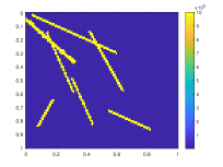
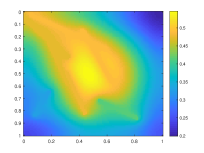
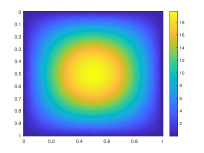
Figure 5.1: Left: $\kappa$. Middle: reference solution at the final time. Right: $f$.

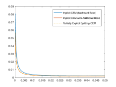
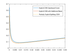
Figure 5.2: Example 1. First type of $V_{2,H}$ (CEM Dof: $300$, $V_{2,H}$ Dof: $243$). Left: $L_{2}$ error. Right: Energy error. Along $x$-axis is time, along $y$-axis is the relative error.

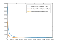
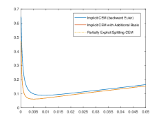
Figure 5.3: Example 1. Second type of $V_{2,H}$ (CEM Dof: $300$, $V_{2,H}$ Dof: $300$). Left: $L_{2}$ error. Right: Energy error. Along $x$-axis is time, along $y$-axis is the relative error.

Numerical Example 2

The medium parameter $\kappa$, the reference solution at final time $u_{ref}$, and the source term $f$ are shown in Figure 5.4. We note that we intentionally choose a singular source term so that CEM with additional basis functions can give a substantial improvement as original multiscale CEM basis functions do not take into account singular source term. In this case, CEM-GMsFEM errors are large. First, we numerically compute the constant $C_{1}$ from (4.12) that is assumed to be independent of the contrast. The result is shown in Table LABEL:tab:constant1 . As we see from this table that as we increase the contrast, this constant remains constant, which asserts that our assumption is true. Next, present numerical results.

In Figure 5.5, we present numerical results (the errors due to discretization), when $V_{2,H}$ is chosen as the first type. Again, we note that because of singular source term, CEM with additional basis functions will provide a visible improvement over CEM without using additional basis functions. This is clear from the figure as we compare blue line (CEM without additional basis functions) and other lines (which coincide) that indicate results obtained using CEM with additional basis functions. The two graphs that coincide correspond results using backward Euler and partially explicit CEM-GMsFEM method with additional basis functions. As we show that the errors are almost the same and thus, one can use our proposed approach with the time step independent of the contrast and with partial explicit strategy. In Figure 5.6, we present results using $V_{2,H}$ as the second type. As we see, our results confirm that this space also provides numerical accuracy as in the first type $V_{2,H}$.

$\cfrac{\max\{\kappa\}}{\min\{\kappa\}}$	$10^{5}$	$10^{6}$	$10^{7}$	$10^{8}$	$10^{9}$
$\sup_{v\in V_{1,H}}\mathcal{G}(v)$	$4.11\times 10^{5}$	$4.11\times 10^{6}$	$4.11\times 10^{7}$	$4.11\times 10^{8}$	$4.11\times 10^{9}$
First type of $V_{2,H}$. $\sup_{v\in V_{2,H}}\mathcal{G}(v)$	$1.75\times 10^{2}$	$1.75\times 10^{2}$	$1.75\times 10^{2}$	$1.75\times 10^{2}$	$1.75\times 10^{2}$
Second type of $V_{2,H}$. $\sup_{v\in V_{2,H}}\mathcal{G}(v)$	$1.40\times 10^{2}$	$1.40\times 10^{2}$	$1.40\times 10^{2}$	$1.40\times 10^{2}$	$1.40\times 10^{2}$

Table 1: Example 2. $\sup\cfrac{\|v\|_{a}^{2}}{\|v\|_{L^{2}}^{2}}$ for different $\cfrac{\max\{\kappa\}}{\min\{\kappa\}}$. Here, we denote $\mathcal{G}(v)=\cfrac{\|v\|_{a}^{2}}{H^{-2}\|v\|_{L^{2}}^{2}}$.

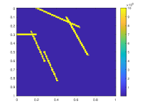
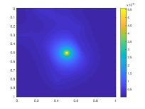
Figure 5.4: Left: $\kappa$. Middle: reference solution at the final time. Right: $f$.

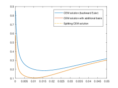
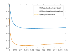
Figure 5.5: Example 2. First type of $V_{2,H}$ (CEM Dof: $300$, $V_{2,H}$ Dof: $243$). Left: $L_{2}$ error. Right: Energy error. Along $x$-axis is time, along $y$-axis is the relative error.

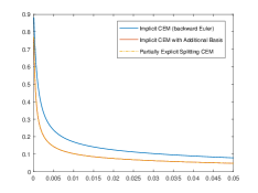
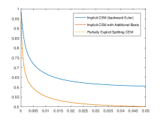
Figure 5.6: Example 2. Second type of $V_{2,H}$ (CEM Dof: $300$, $V_{2,H}$ Dof: $300$). Left: $L_{2}$ error. Right: Energy error. Along $x$-axis is time, along $y$-axis is the relative error.

Numerical Example 3

For our final numerical test, we take more complicated permeability field as shown in Figure 5.7 (more high conductivity streaks). In this figure, we also depict the reference solution at final time $u_{ref}$, and the source term $f$ are shown in the following figure. Because of a singular source term, as before, CEM-GMsFEM with additional basis functions can give a noticeable improvement as original multiscale CEM basis functions do not take into account singular source term. First, we numerically compute the constant from (4.12) that is assumed to be contrast independent. The result is shown in Table 2. As we see from this table that as we increase the contrast, the constant remains constant, which asserts that our assumption is true. Next, present numerical results.

Next, we present numerical results for two types of $V_{2,H}$, as before. We briefly describe one of them as the results are similar. In Figure 5.8 (and Figure 5.9 for second type $V_{2,H}$), we present the errors ($L_{2}$ and energy errors) for CEM without additional basis functions (blue curve) and CEM-GMsFEM with additional basis functions. We show CEM-GMsFEM with additional basis functions that use fully implicit setting and CEM-GMsFEM with those additional basis functions that use partially explicit setting coincide.

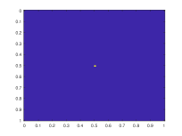
Figure 5.7: Left: $\kappa$, Middle: reference solution at the final time. Right: $f$.

$\cfrac{\max\{\kappa\}}{\min\{\kappa\}}$	$10^{5}$	$10^{6}$	$10^{7}$	$10^{8}$	$10^{9}$
$\sup_{v\in V_{1,H}}\mathcal{G}(v)$	$1.13\times 10^{6}$	$1.13\times 10^{7}$	$1.13\times 10^{8}$	$1.13\times 10^{9}$	$1.13\times 10^{10}$
First type of $V_{2,H}$. $\sup_{v\in V_{2,H}}\mathcal{G}(v)$	$1.78\times 10^{2}$	$1.78\times 10^{2}$	$1.76\times 10^{2}$	$1.76\times 10^{2}$	$1.76\times 10^{2}$
Second type of $V_{2,H}$. $\sup_{v\in V_{2,H}}\mathcal{G}(v)$	$1.35\times 10^{2}$	$1.35\times 10^{2}$	$1.35\times 10^{2}$	$1.35\times 10^{2}$	$1.35\times 10^{2}$

Table 2: Example 2. $\sup\cfrac{\|v\|_{a}^{2}}{\|v\|_{L^{2}}^{2}}$ for different $\cfrac{\max\{\kappa\}}{\min\{\kappa\}}$. Here, we denote $\mathcal{G}(v)=\cfrac{\|v\|_{a}^{2}}{H^{-2}\|v\|_{L^{2}}^{2}}$.

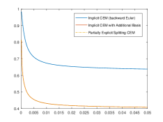
Figure 5.8: Example 3. First type of $V_{2,H}$ (CEM Dof: $300$, $V_{2,H}$ Dof: $243$). Left: $L_{2}$ error. Right: Energy error. Along $x$-axis is time, along $y$-axis is the relative error.

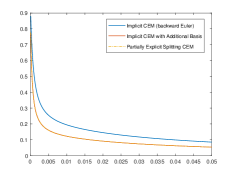
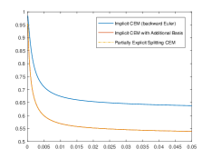
Figure 5.9: Example 2. Second type of $V_{2,H}$ (CEM Dof: $300$, $V_{2,H}$ Dof: $300$). Left: $L_{2}$ error. Right: Energy error. Along $x$-axis is time, along $y$-axis is the relative error.

6 Conclusions

In this paper, we study the development of temporal discretizations that can use time stepping independent of the contrast. We consider a parabolic equation, where the coefficient is multiscale and have high contrast features. We propose a partially explicit method, where the proposed method is stable with the time step that doesnt depend on the contrast. The development of the proposed method requires special multiscale basis construction and temporal splitting. Our coarse space consists of CEM-GMsFEM basis functions and special multiscale basis functions for the remaining degrees of freedom are constructed. The coarse-grid component of the solution (that has a few degrees of freedom) is solved implicitly with explicit contributions from the rest. The remaining part is updated in an explicit fashion within proposed splitting algorithms. We show that the resulting approach is stable with the time step is independent of the contrast. Appropriate multiscale decomposition of the space is needed for the success of the approach as shown in the paper. We formulate sufficient conditions for the decomposition and construct appropriate spatial decomposition. We present numerical results. Our numerical results show that the proposed partial explicit methods give almost the same accuracy as fully implicit method.

Appendix A Motivation for $V_{H,2}$ based on approximation errors

In this appendix, we discuss some motivations of the choices of $V_{H,2}$ based on error reduction viewpoint.

A.1 First choice

We consider the first choice presented in Section 4.2.1. For simplicity, we let $V_{H,1}=V_{glo}$, where $V_{glo}$ is the CEM space defined in (4.3). We consider the elliptic problem: find $u\in V$ such that

$$a(u,v)=(f,v),\quad\forall v\in V.$$

The corresponding multiscale problem is: find $u_{H}:=u_{H,1}+u_{H,2}\in V_{H,1}+V_{H,2}$ such that

$$a(u_{H},v)=(f,v),\quad\forall v\in V_{H,1}+V_{H,2}.$$

Subtracting the above two equations, we obtain

$$a(u-u_{H},v)=0,\quad\forall v\in V_{H,1}+V_{H,2}.$$

Recall that $V=V_{H,1}+\tilde{V}$, $V_{H,1}$ and $\tilde{V}$ are $a$-orthogonal, and that $V_{H,2}\subset\tilde{V}$. So, we have

$$a(u-u_{H,1},v)=0,\quad\forall v\in V_{H,1},$$

which implies that $u-u_{H,1}\in\tilde{V}$. Taking the test function $v\in V_{H,2}$, we obtain

$$a(u_{H,2},v)=a(u-u_{H,1},v),\quad\forall v\in V_{H,2}.$$

From this equation, we see that $V_{H,2}$ provides a correction of the solution $u_{H,1}$ based on the residual $a(u-u_{H,1},v)$.

To derive an error bound, we note that

$$\|u-u_{H,1}\|_{a}^{2}=a(u-u_{H,1},u-u_{H,1})=a(u-u_{H,1},u)=(f,u-u_{H,1}).$$

Using the definition of the $s$-norm defined in Section 4.1, we have

$$(f,u-u_{H,1})\leq CH\|\kappa^{-\frac{1}{2}}f\|\|u-u_{H,1}\|_{s}.$$

Using the fact that $u-u_{H,1}\in\tilde{V}$ and the spectral problem (4.1), we obtain

$$\|u-u_{H,1}\|_{s}^{2}\leq(\min_{i}\lambda_{L_{i}+1}^{(i)})^{-1}\|u-u_{H,1}\|_{a}^{2}.$$

Combining the results, we obtain the following energy norm error bound

$$\|u-u_{H,1}\|_{a}\leq CH(\min_{i}\lambda_{L_{i}+1}^{(i)})^{-\frac{1}{2}}\|\kappa^{-\frac{1}{2}}f\|.$$

To get a $L^{2}$ error bound, we consider the dual problem: given $g\in L^{2}(\Omega)$, find $z\in V$ such that

$$a(v,z)=(g,v),\quad\forall v\in V.$$

The corresponding multiscale problem is given by: find $z_{H}\in V_{H,1}$ such that

$$a(v,z_{H})=(g,v),\quad\forall v\in V_{H,1}.$$

Let $g=\kappa(u-u_{H,1})$. We have

$$\begin{split}\|\kappa^{\frac{1}{2}}(u-u_{H,1})\|^{2}&=(g,u-u_{H,1})=a(u-u_{H,1},z)=a(u-u_{H,1},z-z_{H})\\ &\leq\|u-u_{H,1}\|_{a}\|z-z_{H}\|_{a}\leq C^{2}H^{2}(\min_{i}\lambda_{L_{i}+1}^{(i)})^{-1}\|\kappa^{-\frac{1}{2}}f\|\|\kappa^{\frac{1}{2}}(u-u_{H,1})\|.\end{split}$$

So, we obtain

$$\|\kappa^{\frac{1}{2}}(u-u_{H,1})\|\leq C^{2}H^{2}(\min_{i}\lambda_{L_{i}+1}^{(i)})^{-1}\|\kappa^{-\frac{1}{2}}f\|.$$

Now, we derive the full error $\|u-(u_{H,1}+u_{H,2})\|_{a}$. Note that $u_{H,2}$ is the $a$-orthogonal projection of $u-u_{H,1}$ in the space $V_{H,2}$. So,

$$\|u-(u_{H,1}+u_{H,2})\|_{a}\leq\|u-u_{H,1}-v\|_{a},\quad\forall v\in V_{H,2}.$$

Assume the domain $\Omega$ is rectangular and the mesh $\mathcal{T}_{H}$ is a regular grid. Let $\{\chi_{i}\}$ be a set of smooth partition of unity functions corresponding to the overlapping partition $\cup\{\omega_{i}\}$ of $\Omega$ with $|\nabla\chi_{i}|\leq CH^{-1}$, and that each $\chi_{i}$ has zero trace on $\partial\omega_{i}$. We write

$$u-u_{H,1}=\sum_{i}\chi_{i}(u-u_{H,1})=\sum_{i}r_{i}$$

where $r_{i}=\chi_{i}(u-u_{H,1})$. We assume that the eigenfunctions of (4.5) forms a complete basis, so that each $r_{i}$ can be represented by

$$r_{i}=\sum_{j}a(r_{i},\xi_{j}^{(i)})\xi_{j}^{(i)}$$

where we also assume the normalized condition $a(\xi_{j}^{(i)},\xi_{j}^{(i)})=1$. We define

$$v:=\sum_{i}v_{i}:=\sum_{i}\sum_{j\leq J_{i}}a(r_{i},\xi_{j}^{(i)})\xi_{j}^{(i)}\in V_{H,2}.$$

So, we have

$$\|u-(u_{H,1}+u_{H,2})\|^{2}_{a}\leq 4\sum_{i}\|r_{i}-v_{i}\|_{a}^{2}.$$

Define $0\leq\theta\leq 1$ by

$$\theta=\max_{i}\cfrac{\|r_{i}-v_{i}\|_{a}}{\|r_{i}\|_{a}}$$

which represents relative reduction of error. Notice that

$$\sum_{i}\|r_{i}\|_{a}^{2}\leq 8\|u-u_{H,1}\|_{a}^{2}+8\|u-u_{H,1}\|_{s}^{2}\leq 16C^{4}H^{2}(\min_{i}\lambda_{L_{i}+1}^{(i)})^{-2}\|\kappa^{-\frac{1}{2}}f\|^{2}.$$

Combining all results, we obtain the following error bound

$$\|u-(u_{H,1}+u_{H,2})\|_{a}\leq C_{0}\theta H(\min_{i}\lambda_{L_{i}+1}^{(i)})^{-1}\|\kappa^{-\frac{1}{2}}f\|.$$

A.2 Second choice

We consider the second choice in this section. We consider an estimate of the elliptic projection of $V_{glo}+V_{glo,2}$ with second choice of $V_{glo,2}$. Specifically, we assume $u_{1}\in V_{glo}$, $u_{2}\in V_{glo,2}$ and $u\in V$ satisfy

$$a(u,v)=(f,v),\;\;\forall v\in V,$$

and

$$a(u_{1}+u_{2},v_{1}+v_{2})=(f,v_{1}+v_{2}),\;\;\forall v_{1}\in V_{glo},v_{2}\in V_{glo,2}.$$

We define $\overline{V}=\{v\in V|\;\tilde{\Pi}(v)=0\}$ and we can easy check that $\overline{V}$ is $a$-orthogonal to $V_{glo,1}+V_{glo,2}$, namely $(V_{glo}+V_{glo,2})\subset\overline{V}^{\perp_{a}}$. where $\overline{V}^{\perp_{a}}$ is the orthogonal complement of $\overline{V}$ with respect to the $a(\cdot,\cdot)$ inner product. By counting the dimension of $\overline{V}^{\perp_{a}}$ and $V_{glo}+V_{glo,2}$, we have

$$(V_{glo,1}+V_{glo,2})=\overline{V}^{\perp_{a}}\text{ and }(V_{glo}+V_{glo,2})^{\perp_{a}}=\overline{V}.$$

Since

$$a(u-u_{1}-u_{2},v)=0,\;\;\forall v\in V_{glo}+V_{glo,2},$$

we have

$$u-u_{1}-u_{2}\in(V_{glo}+V_{glo,2})^{\perp_{a}}=\overline{V}.$$

Thus, we have

$$a(u-u_{1}-u_{2},u-u_{1}-u_{2}) =a(u,u-u_{1}-u_{2})=(f,u-u_{1}-u_{2})$$

$$\leq\|f\|\|(u-u_{1}-u_{2})\|.$$

Note that $\overline{V}\subset\tilde{V}$. Since $u-u_{1}-u_{2}\in\overline{V}$, we can write $u-u_{1}-u_{2}$ in terms of the eigenfunctions of (4.7),

$$u-u_{1}-u_{2}=\sum_{i=1}\sum^{\infty}_{j=1}a^{(i)}_{j}\xi^{(i)}_{j}.$$

Since $u-u_{1}-u_{2}\in\overline{V}\subset\tilde{V}$, we have

$$a^{(i)}_{j}=0\;\forall j\leq J_{i},$$

which implies

$$u-u_{1}-u_{2}=\sum_{i=1}\sum^{\infty}_{j=J_{i}+1}a^{(i)}_{j}\xi^{(i)}_{j}.$$

So, we have

$$H^{-2}\|(u-u_{1}-u_{2})\|^{2}_{L^{2}} =\sum_{i=1}\sum^{\infty}_{j=J_{i}+1}(a^{(i)}_{j})^{2}\leq\sum_{i=1}(\gamma^{(i)}_{J_{i}+1})^{-1}\sum^{\infty}_{j=J_{i}+1}\gamma^{(i)}_{j}(a^{(i)}_{j})^{2}$$

$$\leq(\min_{i}\gamma^{(i)}_{J_{i}+1})^{-1}\sum_{i=1}\sum^{\infty}_{j=J_{i}+1}\gamma^{(i)}_{j}(a^{(i)}_{j})^{2}$$

$$\leq(\min\{\gamma_{J_{i}+1}^{(i)}\})^{-1}\|u-u_{1}-u_{2}\|^{2}_{a}$$

and

$$\|(u-u_{1}-u_{2})\|_{L^{2}} \leq\cfrac{H}{(\min\{\gamma_{J_{i}+1}^{(i)}\})^{\frac{1}{2}}}\|u-u_{1}-u_{2}\|_{a}.$$

Therefore, we have

$$\|u-u_{1}-u_{2}\|_{a}\leq\cfrac{H\|f\|_{L^{2}}}{(\min\{\gamma_{J_{i}+1}^{(i)}\})^{\frac{1}{2}}}.$$

We remark that for the standard CEM method, we have the error estimate

$$\|u-u_{1}-u_{2}\|_{a}\leq\cfrac{H\|\kappa^{-\frac{1}{2}}f\|_{L^{2}}}{(\min\{\lambda_{L_{i}+1}^{(i)}\})^{\frac{1}{2}}}.$$

By the definition of the $s$-norm, we have

$$\|v\|^{2}_{s}\geq C\kappa_{min}H^{-2}\|v\|^{2}$$

where we use the fact that $\sum_{i}|\nabla\chi_{i}|^{2}\leq CH^{-2}$. So,

$$\gamma_{J_{i}+1}^{(i)}\geq\gamma_{1}^{(i)}=\min_{v\in\tilde{V}}\cfrac{\|v\|_{a}^{2}}{H^{-2}\|v\|_{L^{2}}^{2}}\geq C\kappa_{min}\min_{v\in\tilde{V}}\cfrac{\|v\|_{a}^{2}}{\|v\|_{s}^{2}}=C\kappa_{min}\lambda_{L_{i}+1}^{(i)}.$$

Thus, the enriched space $V_{H,2}$ can improve the elliptic projection error from $O(\cfrac{H}{(\min\{\lambda_{L_{i}+1}^{(i)}\})^{\frac{1}{2}}})$ to $O(\cfrac{H}{(\min\{\gamma_{J_{i}+1}^{(i)}\})^{\frac{1}{2}}})$.

References

- [1] A. Abdulle. Explicit methods for stiff stochastic differential equations. In Numerical Analysis of Multiscale Computations, pages 1–22. Springer, 2012.
- [2] J. Aldaz. Strengthened Cauchy-Schwarz and Hölder inequalities. arXiv preprint arXiv:1302.2254, 2013.
- [3] G. Ariel, B. Engquist, and R. Tsai. A multiscale method for highly oscillatory ordinary differential equations with resonance. Mathematics of Computation, 78(266):929–956, 2009.
- [4] U. M. Ascher, S. J. Ruuth, and R. J. Spiteri. Implicit-explicit runge-kutta methods for time-dependent partial differential equations. Applied Numerical Mathematics, 25(2-3):151–167, 1997.
- [5] D. L. Brown, Y. Efendiev, and V. H. Hoang. An efficient hierarchical multiscale finite element method for stokes equations in slowly varying media. Multiscale Modeling & Simulation, 11(1):30–58, 2013.
- [6] E. T. Chung, Y. Efendiev, and T. Hou. Adaptive multiscale model reduction with generalized multiscale finite element methods. Journal of Computational Physics, 320:69–95, 2016.
- [7] E. T. Chung, Y. Efendiev, and C. Lee. Mixed generalized multiscale finite element methods and applications. SIAM Multiscale Model. Simul., 13:338–366, 2014.
- [8] E. T. Chung, Y. Efendiev, and W. T. Leung. Generalized multiscale finite element methods for wave propagation in heterogeneous media. Multiscale Modeling & Simulation, 12(4):1691–1721, 2014.
- [9] E. T. Chung, Y. Efendiev, and W. T. Leung. Residual-driven online generalized multiscale finite element methods. Journal of Computational Physics, 302:176–190, 2015.
- [10] E. T. Chung, Y. Efendiev, and W. T. Leung. Constraint energy minimizing generalized multiscale finite element method. Computer Methods in Applied Mechanics and Engineering, 339:298–319, 2018.
- [11] E. T. Chung, Y. Efendiev, and W. T. Leung. Constraint energy minimizing generalized multiscale finite element method in the mixed formulation. Computational Geosciences, 22(3):677–693, 2018.
- [12] E. T. Chung, Y. Efendiev, and W. T. Leung. Fast online generalized multiscale finite element method using constraint energy minimization. Journal of Computational Physics, 355:450–463, 2018.
- [13] E. T. Chung, Y. Efendiev, W. T. Leung, M. Vasilyeva, and Y. Wang. Non-local multi-continua upscaling for flows in heterogeneous fractured media. Journal of Computational Physics, 372:22–34, 2018.
- [14] W. E and B. Engquist. Heterogeneous multiscale methods. Comm. Math. Sci., 1(1):87–132, 2003.
- [15] Y. Efendiev, J. Galvis, and T. Hou. Generalized multiscale finite element methods (GMsFEM). Journal of Computational Physics, 251:116–135, 2013.
- [16] Y. Efendiev and T. Hou. Multiscale Finite Element Methods: Theory and Applications, volume 4 of Surveys and Tutorials in the Applied Mathematical Sciences. Springer, New York, 2009.
- [17] Y. Efendiev, S. Pun, and P. N. Vabishchevich. Temporal splitting algorithms for non-stationary multiscale problems. arXiv preprint, 2020.
- [18] Y. Efendiev and P. N. Vabishchevich. Splitting methods for solution decomposition in nonstationary problems. arXiv preprint arXiv:2008.08111, 2020.
- [19] B. Engquist and Y.-H. Tsai. Heterogeneous multiscale methods for stiff ordinary differential equations. Mathematics of computation, 74(252):1707–1742, 2005.
- [20] P. Henning, A. Målqvist, and D. Peterseim. A localized orthogonal decomposition method for semi-linear elliptic problems. ESAIM: Mathematical Modelling and Numerical Analysis, 48(5):1331–1349, 2014.
- [21] T. Hou and X. Wu. A multiscale finite element method for elliptic problems in composite materials and porous media. J. Comput. Phys., 134:169–189, 1997.
- [22] T. Y. Hou, D. Huang, K. C. Lam, and P. Zhang. An adaptive fast solver for a general class of positive definite matrices via energy decomposition. Multiscale Modeling & Simulation, 16(2):615–678, 2018.
- [23] T. Y. Hou, Q. Li, and P. Zhang. Exploring the locally low dimensional structure in solving random elliptic pdes. Multiscale Modeling & Simulation, 15(2):661–695, 2017.
- [24] T. Y. Hou, D. Ma, and Z. Zhang. A model reduction method for multiscale elliptic pdes with random coefficients using an optimization approach. Multiscale Modeling & Simulation, 17(2):826–853, 2019.
- [25] P. Jenny, S. Lee, and H. Tchelepi. Multi-scale finite volume method for elliptic problems in subsurface flow simulation. J. Comput. Phys., 187:47–67, 2003.
- [26] C. Le Bris, F. Legoll, and A. Lozinski. An MsFEM type approach for perforated domains. Multiscale Modeling & Simulation, 12(3):1046–1077, 2014.
- [27] M. Li, E. Chung, and L. Jiang. A constraint energy minimizing generalized multiscale finite element method for parabolic equations. Multiscale Modeling & Simulation, 17(3):996–1018, 2019.
- [28] T. Li, A. Abdulle, et al. Effectiveness of implicit methods for stiff stochastic differential equations. In Commun. Comput. Phys. Citeseer, 2008.
- [29] G. I. Marchuk. Splitting and alternating direction methods. Handbook of numerical analysis, 1:197–462, 1990.
- [30] H. Owhadi and L. Zhang. Metric-based upscaling. Comm. Pure. Appl. Math., 60:675–723, 2007.
- [31] A. Roberts and I. Kevrekidis. General tooth boundary conditions for equation free modeling. SIAM J. Sci. Comput., 29(4):1495–1510, 2007.
- [32] G. Samaey, I. Kevrekidis, and D. Roose. Patch dynamics with buffers for homogenization problems. J. Comput. Phys., 213(1):264–287, 2006.
- [33] A. A. Samarskii. The Theory of Difference Schemes. Marcel Dekker, New York, 2001.
- [34] A. A. Samarskii, P. P. Matus, and P. N. Vabishchevich. Difference Schemes with Operator Factors. Kluwer Academic Pub, 2002.
- [35] P. N. Vabishchevich. Additive Operator-Difference Schemes: Splitting Schemes. Walter de Gruyter GmbH, Berlin, Boston, 2013.