CQUeST-2020-0655

Shadow cast by a rotating black hole with anisotropic matter

$\mbox{Bum-Hoon Lee}^{\S{\dagger}}$,   $\mbox{Wonwoo Lee}^{\S}$,    $\mbox{Yun Soo Myung}^{\P}$

§Center for Quantum Spacetime, Sogang University, Seoul 04107, Korea
†Department of Physics, Sogang University, Seoul 04107, Korea
¶Institute of Basic Sciences and Department of Computer Simulation, Inje University,
Gimhae 50834, Korea

Abstract

We obtain the shadow cast induced by the rotating black hole with an anisotropic matter. A Killing tensor representing the hidden symmetry is derived explicitly. The existence of a separability structure implies complete integrability of the geodesic motion. We analyze an effective potential around the unstable circular photon orbits to show that one side of the black hole is brighter than the other side. Further, it is shown that the inclusion of the anisotropic matter ($Kr^{2(1-w)}$) has an effect on the observables of the shadow cast. The shadow observables include approximate shadow radius $R_{s}$, distortion parameter $\delta_{s}$, area of the shadow $A_{s}$, and oblateness $D_{os}$.

1 Introduction

It is interesting to note that a black hole is one of the fascinating and mystical objects in the universe. Its physical meaning and existence as a real object have developed over the past century [1, 2, 3, 4, 5, 6, 7, 8]. It is fair to say that black holes do not seem to be directly observed. Therefore, they have been proved by indirect observations like the deflection of light rays due to the spacetime curvature [9, 10, 11, 12], or the gravitational wave by coming from the mergers of compact binary sources [13, 14].

Interestingly, the black hole has recently gained the most attention thanks to the observational reports on the shadow cast induced by the supermassive black hole [15, 16, 17] at the center of the M87 galaxy obtained by the Event Horizon Telescope collaboration [18, 19, 20]. The shadow image indicates the bright ring surrounding a dark region in the celestial sphere. The dark area describing the black hole shadow has the boundary between capture orbits and scattering orbits by photons in which photons are coming from both the accreting disc and the light source located behind a black hole, and they reach a distant observer [21, 22, 23, 24, 25, 26, 27, 28].

Let us propose an astrophysical black hole residing in the background of matters. In this case, it is appropriate to consider a realistic black hole surrounded by a matter field or dark matter. It is well-known that dark matter [29, 30, 31, 32] makes up about $27\%$ of the universe and more than $90\%$ of the matter in the Milky Way. To model a black hole in the galaxy, it is reasonable to consider the black hole coexisting with matter field or dark matter [33, 34, 35].

Analyzing the geodesic motion of a photon outside the black hole horizon is an important matter when studying astrophysical objects exposed to observations. Theoretically, studying the geodesic motion of a photon may provide a clear picture of geometrical properties for the neighborhood of a rotating black hole [36]. One may construct astrophysical models exposed to observations by describing the geodesic motion [21]. Actually, the black hole shadow could be investigated by analyzing the null geodesics around the rotating black hole.

The black hole shadow could be used to measure physical parameters (mass, charge, angular momentum, inclination angle, structure of the accretion disk). All parameters may include the effects of the black hole surrounded with matter fields or those in modified gravity theories. For this reason, the shadow cast has been extensively investigated in gravity theory with/without matter fields [21, 23, 37, 38, 39, 40, 41, 42, 43, 44, 45, 46, 47, 48, 49, 50, 51, 52, 53, 54, 55, 56], other rotating objects [57, 58, 59, 60], and modified gravity theories [61, 62, 63, 64, 65, 66, 67, 68, 69, 70, 71, 72, 73, 74].

Recently, two of us have obtained the rotating black hole solution with an anisotropic matter [35] where the anisotropic matter with parameters $w$ and $K$ may describe both an extra U(1) field [75, 62, 76, 77, 78] and diverse dark matters. It is shown that this black hole geometry can affect the shadow when comparing with Kerr and Kerr-Newman black holes [51]. We are also interested in studying the shadow cast induced by the black hole with an anisotropic matter as a subsequent study. For this purpose, we will derive the Killing tensor and find the separability structure to guarantee the integrability of the geodesic motions. Also, we investigate an effective potential for unstable circular photon orbits to show that one side of the black hole is brighter than the other side. As additional shadow observables, we analyze the approximate shadow radius and distortion parameter. We hope that all may have a complementary relationship with one another, to describe the nature.

In this work, we wish to focus on studying the shadow cast induced by the black hole with an anisotropic matter. The paper is organized as follows. In Sec. $2$, we explore the symmetry of the rotating black hole geometry [79]. A Killing tensor representing the hidden symmetry is constructed and the separability structure exists. In Sec. $3$, we derive the geodesic equation by adopting the Hamilton-Jacobi formalism. To get the information on the boundary of the shadow cast, we study the radial null geodesic motion by making use of the effective potential. In Sec. $4$, we employ a backward ray-tracing algorithm [80, 81, 82] to analyze the shadow cast induced by a rotating black hole with an anisotropic matter field described by two parameters $w$ and $K$. We present the apparent shape of shadow and observables characterizing the shadow. We observe that the anisotropic matter field with $w$ influences on the observables. Finally, we summarize our results and discuss on relevant matters in Sec. $5$.

2 Symmetry and separability structure

First of all, we consider the action

$$I=\int d^{4}x\sqrt{-g}\Big{[}\frac{1}{16\pi}(R-F_{\mu\nu}F^{\mu\nu})+{\cal L}_{\rm am}\Big{]}+I_{b},$$ (1)

where ${\cal L}_{\rm am}$ describes effective anisotropic matter fields and $I_{b}$ is the boundary term [83, 84]. The rotating black hole solution with an anisotropic matter is obtained by applying the Newman-Janis algorithm to a static spherically symmetric solution as [35]

$$ds^{2}=-F(r,\theta)dt^{2}-2[1-F(r,\theta)]a\sin^{2}\theta dtd\phi+\frac{\Sigma}{\rho^{2}}\sin^{2}\theta d\phi^{2}+\frac{\rho^{2}}{\triangle}dr^{2}+\rho^{2}d\theta^{2}\,,$$ (2)

where

$$F(r,\theta) = 1-\frac{2Mr-Q^{2}+Kr^{2(1-w)}}{\rho^{2}},\quad a=\frac{J}{M},\quad\rho^{2}=r^{2}+a^{2}\cos^{2}\theta,$$

$$\triangle = r^{2}+a^{2}+Q^{2}-2Mr-Kr^{2(1-w)},$$

$$\Sigma = \rho^{2}(r^{2}+a^{2})+(2Mr-Q^{2}+Kr^{2(1-w)})a^{2}\sin^{2}\theta.$$ (3)

It is important to point out that the parameters $K$ and $w$ control the density and anisotropy of the fluid matter surrounding the black hole. The $K=0$ case leads to the Kerr-Newman black hole and $K=0$ with $Q=0$ corresponds to the Kerr black hole, regarding as two reference black holes. This includes the rotating version of the Reissner-Nordström black hole with the constant scalar hair [77] characterized by $K<0$, $w=1$, and $a=0$. The metric is asymptotically flat for $w>0$ only. For $0\leq w\leq 1/2$, the energy density is not localized sufficiently such that the total energy diverges [35]. Thus, we consider the case with $w>1/2$ to obtain the geometry including a finite total energy with asymptotically flat spacetime. We allow $K$ to take either sign for representing diverse matters surrounding the rotating black hole.

At this stage, we mention that the event (outer) horizon ($r_{H}$) for the spacetime (2) is located at the largest radius as a solution to $\triangle=0$, leading to the event horizon for Kerr-Newman black hole with $K=0$.

We are interested particularly in the ergosphere for later use in Sec. 3. The ergosphere is defined as a region between surface of static limit (infinite redshift) and outer horizon [85]. On the surface, the timelike Killing vector becomes null-like as $g_{tt}=0$. Let us consider a photon emitted in the $\phi$ direction at radius $r$ without $r$ and $\theta$ momentum components. From the condition of the null trajectory, one obtains two angular velocities

$$\omega_{\pm}=\frac{-g_{t\phi}\pm\sqrt{\triangle\sin^{2}\theta}}{g_{\phi\phi}}\,,$$ (4)

where $\triangle\sin^{2}\theta=g^{2}_{t\phi}-g_{tt}g_{\phi\phi}$. Outside the event horizon ($\triangle>0$), two roots $\omega_{\pm}$ are alive, while there are no real roots inside the horizon. At the static limit surface satisfying $g_{tt}=0$ and $g_{t\phi}<0$, one finds $\omega_{+}=-\frac{2g_{t\phi}}{g_{\phi\phi}}$ and $\omega_{-}=0$. Inside the ergosphere ($g_{tt}>0$), one has $\omega_{-}>0$. Therefore, all particles are necessarily corotating with the rotating black hole. On the event horizon, the two angular velocities appear the same as $\omega_{\pm}=\Omega|_{r=r_{H}}=\frac{a}{r^{2}_{H}+a^{2}}$.

Now, we examine the symmetry and separability structure of the rotating black hole geometry. There are explicit and hidden symmetries related to Killing vectors and Killing tensors, respectively [86, 79]. Killing vectors correspond to the generators of isometries for spacetime geometry. The geometry of (2) implying a stationary axisymmetry, admits two commuting Killing vectors $\xi^{\mu}_{(t)}=\delta^{\mu}_{t}$ and $\xi^{\mu}_{(\phi)}=\delta^{\mu}_{\phi}$ [87]. On the other hand, Killing tensors correspond to a symmetric generalization of Killing vectors. A hidden symmetry represents the geometric structure of spacetime encoded in Killing tensors. This implies that an additional integral of the motion is quadratic in momentum as ${\cal K}^{\mu\nu}p_{\mu}p_{\nu}$ [88]. It is known that one of the Killing tensors is the metric tensor, having the structure of $g^{\mu\nu}p_{\mu}p_{\nu}=-m^{2}$.

We consider the null tetrad [89, 90] to construct the Killing tensor. The null tetrad consists of two real null vectors $l^{\mu}$ and $n^{\mu}$ and two complex null vectors $m^{\mu}$ and ${\bar{m}}^{\mu}$. They satisfy $l^{\mu}n_{\mu}=-1$, $m^{\mu}{\bar{m}}_{\mu}=1$, and $l^{\mu}m_{\mu}=l^{\mu}{\bar{m}}_{\mu}=n^{\mu}m_{\mu}=n^{\mu}{\bar{m}}_{\mu}=0$. For our purpose, we introduce an inverse metric for (2)

$$g^{\mu\nu}=\left(\begin{array}[]{cccc}-\frac{\Sigma}{\triangle\rho^{2}}&0&0&-\frac{a(1-F)}{\triangle}\\ 0&\frac{\triangle}{\rho^{2}}&0&0\\ 0&0&\frac{1}{\rho^{2}}&0\\ -\frac{a(1-F)}{\triangle}&0&0&\frac{\triangle-a^{2}\sin^{2}\theta}{\triangle\rho^{2}\sin^{2}\theta}\end{array}\right).$$

Then, $g^{\mu\nu}$ can be expressed in terms of the null tetrad as

$$g^{\mu\nu}=-l^{\mu}n^{\nu}-n^{\mu}l^{\nu}+m^{\mu}\bar{m}^{\nu}+\bar{m}^{\mu}m^{\nu}\,,$$ (5)

where the null vectors are given by

$$l^{\mu}=\frac{1}{\triangle}\left[(r^{2}+a^{2})\delta^{\mu}_{0}+\triangle\delta^{\mu}_{1}+a\delta^{\mu}_{3}\right]\,,~{}n^{\mu}=\frac{1}{2\rho^{2}}\left[(r^{2}+a^{2})\delta^{\mu}_{0}-\triangle\delta^{\mu}_{1}+a\delta^{\mu}_{3}\right]\,,$$

$$m^{\mu}=\frac{1}{\sqrt{2}(r+ia\cos\theta)}\left[ia\sin\theta\delta^{\mu}_{0}+\delta^{\mu}_{2}+\frac{i}{\sin\theta}\delta^{\mu}_{3}\right]\,,$$

$${\bar{m}}^{\mu}=\frac{1}{\sqrt{2}(r-ia\cos\theta)}\left[-ia\sin\theta\delta^{\mu}_{0}+\delta^{\mu}_{2}-\frac{i}{\sin\theta}\delta^{\mu}_{3}\right]\,.$$ (6)

Importantly, a quadratic Killing tensor is constructed by making use of these null vectors [88, 91]

$${\cal K}^{\mu\nu} = 2\rho^{2}m^{(\mu}{\bar{m}}^{\nu)}-a^{2}\cos^{2}\theta g^{\mu\nu}$$ (7)

$$= a^{2}\sin^{2}\theta\delta^{\mu}_{0}\delta^{\nu}_{0}+2a\delta^{(\mu}_{0}\delta^{\nu)}_{3}+\frac{\delta^{\mu}_{3}\delta^{\nu}_{3}}{\sin^{2}\theta}+\delta^{\mu}_{2}\delta^{\nu}_{2}-a^{2}\cos^{2}\theta g^{\mu\nu}\,,$$

which satisfies $\nabla^{(\alpha}{\cal K}^{\mu\nu)}=0$ and ${\cal K}^{\mu\nu}={\cal K}^{(\mu\nu)}$.

Let us consider the separability structure [92, 93] which describes the separation of variables in the Hamilton-Jacobi formalism. We are aware that there exist two Killing vectors ($\xi^{\mu}_{(t)}$ and $\xi^{\mu}_{(\phi)}$) satisfying $\nabla^{(\alpha}\xi^{\mu)}=0$, and two Killing tensors (${\cal K}^{\mu\nu}$ and $g^{\mu\nu}$). The metric tensor also satisfies $\nabla^{(\alpha}g^{\mu\nu)}=0$ and $g^{\mu\nu}=g^{(\mu\nu)}$. One can show that two Killing tensors mutually commute under the Schouten-Nijenhuis bracket

$$[{\cal K}^{\mu\nu},g^{\mu\nu}]_{\rm SN}=2{\cal K}^{\alpha(\mu}\nabla_{\alpha}g^{\nu\beta)}-2g^{\alpha(\mu}\nabla_{\alpha}{\cal K}^{\nu\beta)}=0\,,$$ (8)

which is regarded as an alternative form of the Killing tensor equation. Also, the Killing tensors and vectors satisfy

$$[\xi^{\mu}_{(t)},{\cal K}^{\mu\nu}]_{\rm SN}={\cal L}_{\xi^{\mu}_{(t)}}{\cal K}^{\mu\nu}=[\xi^{\mu}_{(\phi)},{\cal K}^{\mu\nu}]_{\rm SN}=[\xi^{\mu}_{(t)},g^{\mu\nu}]_{\rm SN}=[\xi^{\mu}_{(\phi)},g^{\mu\nu}]_{\rm SN}=[\xi^{\mu}_{(t)},\xi^{\mu}_{(\phi)}]_{\rm SN}=0\,.$$ (9)

Therefore, we prove that the rotating black hole geometry admits the separability structure. Its existence guarantees a complete integrability of the geodesic motions.

3 Geodesic motions

In this section, we investigate the geodesic motions [94, 95, 96, 97]. For the static spherically symmetric black hole, one can construct four integrals of geodesic motion: test particle’s energy, projection of angular momentum to an arbitrary axis, square of total angular momentum, and normalization of the four-velocity. These are conserved along the geodesics. Therefore, the geodesic equation becomes completely separable. For an axisymmetric rotating black hole, the total angular momentum is not conserved. However, determining the orbit of a test particle is a necessary step to find four integrals of the geodesic motion. In this direction, Carter has obtained the fourth constant by performing the separation of variables in the Hamilton-Jacobi formalism [98]. Here, we wish to construct four independent integrals of the geodesic motion by making use of two Killing vectors and two Killing tensors.

The four integrals of the motion are given by two conserved quantities related to Killing vectors

$$\xi^{\mu}_{(t)}p_{\mu} = -E=-F(r,\theta)\dot{t}-[1-F(r,\theta)]a\sin^{2}\theta\dot{\phi}\,,$$

$$\xi^{\mu}_{(\phi)}p_{\mu} = L_{z}=-[1-F(r,\theta)]a\sin^{2}\theta\dot{t}+\frac{\Sigma\sin^{2}\theta}{\rho^{2}}\dot{\phi}\,,$$ (10)

and two conserved quantities related to Killing tensors

$$g^{\mu\nu}p_{\mu}p_{\nu} = -m^{2}\,,$$

$${\cal K} \equiv {\cal K}^{\mu\nu}p_{\mu}p_{\nu}=p^{2}_{\theta}+(L_{z}-aE\sin^{2}\theta)^{2}/\sin^{2}\theta+a^{2}m^{2}\cos^{2}\theta\,.$$ (11)

Here, we investigate the geodesic motion around the rotating black hole by following the procedure of the separation of variables in the Hamilton-Jacobi formalism [98]. In this case, Carter’s fourth constant of the motion is given by

$${\cal Q}=p^{2}_{\theta}+\cos^{2}\theta[a^{2}(m^{2}-E^{2})+L^{2}_{z}/\sin^{2}\theta]\,,$$ (12)

which represents the separation constant for the $r$ and $\theta$-directions of null geodesics. The constant of the motion is given by

$${\cal Q}+(L_{z}-aE)^{2}=p^{2}_{\theta}+(L_{z}-aE\sin^{2}\theta)^{2}/\sin^{2}\theta+a^{2}m^{2}\cos^{2}\theta\,,$$ (13)

indicating that ${\cal Q}$ may be negative but ${\cal K}$ is always non-negative. Equation (13) has the same form as Eq. (11) implying ${\cal K}\equiv{\cal Q}+(L_{z}-aE)^{2}$.

We notice that the geodesic motion of a neutral particle is described by the Hamilton-Jacobi equation. The geodesic equations as four first-order differential equations are found to be

$$\rho^{2}p^{t}\equiv\rho^{2}\frac{dt}{d\lambda}=-a(aE\sin^{2}\theta-L_{z})+\frac{(r^{2}+a^{2})P(r)}{\triangle}\,,$$ (14)

$$\rho^{2}p^{\phi}\equiv\rho^{2}\frac{d\phi}{d\lambda}=-\left(aE-\frac{L_{z}}{\sin^{2}\theta}\right)+\frac{aP(r)}{\triangle}\,,$$ (15)

$$\rho^{2}p^{r}\equiv\rho^{2}\frac{dr}{d\lambda}=\pm\sqrt{R(r)}=\triangle p_{r}\,,$$ (16)

$$\rho^{2}p^{\theta}\equiv\rho^{2}\frac{d\theta}{d\lambda}=\pm\sqrt{\Theta(\theta)}\,.$$ (17)

Here $+(-)$ in Eqs. (16) and (17) correspond to the outgoing (ingoing) geodesics and

$$\Theta(\theta)={\cal Q}-\cos^{2}\theta[a^{2}(m^{2}-E^{2})+L^{2}_{z}/\sin^{2}\theta],$$ (18)

$$R(r)=P^{2}(r)-\triangle[m^{2}r^{2}+(L_{z}-aE)^{2}+{\cal Q}]\,,$$ (19)

$$P(r)=(r^{2}+a^{2})E-aL_{z}\,.$$ (20)

The geodesic motion of a test particle is not confined in a plane, implying that two effective potentials for the radial and latitudinal motions should be examined separately.

Now we are in a position to study the null geodesic motion with $m=0$. It is noted that the angular size of a light source is much bigger than the angular size of the black hole. They are two important null geodesic motions named as principal congruences and unstable circular orbits. We focus on unstable circular orbits and then, mention the principal congruences briefly. The radial equation for null geodesic is given by

$$\frac{1}{2}\left(\frac{dr}{d\lambda}\right)^{2}+V_{\rm eff}(r)=0\,,$$ (21)

where the effective potential in the equatorial plane is given by

$$V_{\rm eff}(r)=-\frac{((r^{2}+a^{2})^{2}-\triangle a^{2})E^{2}-2aL_{z}(r^{2}+a^{2}-\triangle)E+(a^{2}-\triangle)L^{2}_{z}}{2r^{4}}\,.$$ (22)

Here, we note that Carter’s constant of the motion $({\cal Q})$ disappears. The local maximum in the effective potentials determines the radii of unstable circular photon orbits. For $K=0$, this reduces to the Kerr-Newman potential

$$V^{\rm KN}_{\rm eff}(r)=-\frac{[r^{2}(r^{2}+a^{2})+a^{2}(2Mr-Q^{2})]E^{2}-2aL_{z}(2Mr-Q^{2})E+(-r^{2}+2Mr-Q^{2})L^{2}_{z}}{2r^{4}}.$$ (23)

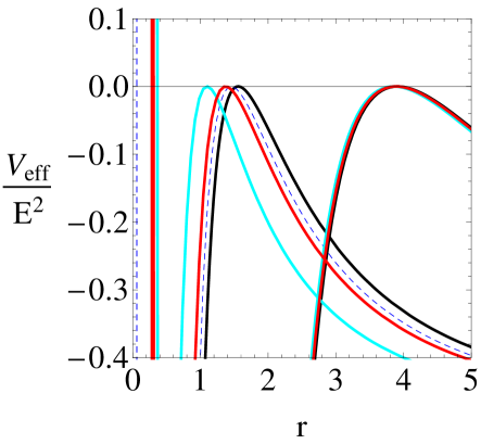
(a) Effective potentials

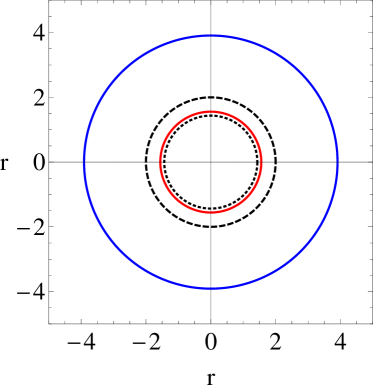
(b) Locations of unstable circular orbits

Figure 1: (color online). Effective potentials and locations of unstable circular orbits in the equatorial plane.

For unstable circular orbits, we have to take into account $V_{eff}=0$ and $\frac{dV_{eff}}{dr}=0$. Solving these, the location of a peak is determined as

$$r_{uco} = \frac{L_{z}-aE}{L_{z}+aE}\Big{[}3M-\frac{2Q^{2}}{r_{uco}}+K(1+w)r^{(1-2w)}_{uco}\Big{]}\,.$$ (24)

For $K=0$, this reduces to the Kerr-Newman case. For photon circular orbits around the extremal Kerr black hole with $a=M$, one has either $r_{\rm uco-}=M$ (corotating) or $r_{\rm uco+}=4M$ (counterrotating case).

Carter’s constant determines the test particle’s motion in the $\theta$-direction [99, 100]. A physically arrowed region is defined by $\Theta(\theta)\geq 0$. The orbits cross the equatorial plane repeatedly for ${\cal Q}>0$, while they remain in the equatorial plane for ${\cal Q}=0$. We have the condition of ${\cal Q}<0$ for the principal null congruences.

We introduce the dimensionless quantities ($\bar{a}=a/M$, $\bar{Q}=Q/M$, $\bar{K}=K/M^{2w}$, $\bar{r}=r/M$). Hereafter, we will remove the bar for simplicity.

Figure 1(a) shows the effective potential for both corotating and counterrotating cases in the equatorial plane. The left concave curves correspond to the former case, while the right concave curves to the latter case. As reference curves, black curves correspond to the Kerr one with $a=0.9$, blue dashed curves to Kerr-Newman one [101] with $Q=0.25$. For our work, we note that red curves denote the case with $a=0.9$, $Q=0$ $w=3/2$, $K=-0.13$ while cyan curves represent the case with $a=0.9$, $Q=0.25$, $w=3/2$, $K=-0.13$.

Figure 1(b) shows the locations of unstable circular orbits. The black dotted (dashed) circle indicates the location of outer horizon (static limit). The red circle denotes the unstable circle orbit for the corotating case, while the blue circle represents the counterrotating case. We note that the unstable circle orbit for the corotating case is located within the ergosphere, implying that the angular velocity of null rays for the counterrotating case could change the sign in the ergosphere and they move along unstable circle orbit. Hence, the number of photons for corotating case is larger than those for counterrotating case when reaching the distant observer.

Now, let us consider null geodesics along $\theta=\theta_{c}=$const plane. Considering that $\dot{r}$ and $\dot{\theta}$ must be real on the geodesics in Eqs. (16) and (17), one has $R(r)\geq 0$ and $\Theta(\theta)\geq 0$ in Eq. (18). $\Theta(\theta)$ is rewritten as

$$\Theta(\theta)={\cal Q}+(a^{2}E^{2}+L^{2}_{z})-\left(a^{2}E^{2}\sin^{2}\theta+\frac{L^{2}_{z}}{\sin^{2}\theta}\right)\,.$$ (25)

For $\theta=\theta_{c}$, one has

$$\Theta(\theta)|_{\theta=\theta_{c}}=0\,,\quad\partial_{\theta}\Theta(\theta)|_{\theta=\theta_{c}}=0\,.$$ (26)

Equivalently, one finds

$$\frac{L_{z}}{E}=a\sin^{2}\theta_{c}\,,\quad\frac{{\cal Q}}{E^{2}}=-a^{2}\cos^{4}\theta_{c}\,.$$ (27)

If Eq. (27) is satisfied, the solution to the geodesic equations provides the principal null geodesic. From Eqs. (14), (15), and (16) with Eq. (27), we get

$$\frac{dt}{dr}=\pm\frac{r^{2}+a^{2}}{\triangle}\,,\quad\frac{d\phi}{dr}=\pm\frac{a}{\triangle}\,.$$ (28)

The outgoing(+)/ingoing($-$) radial congruences correspond to the two principal null congruences in Boyer-Lindquist coordinates. We may refer Refs. [102, 103, 104, 105] for discussion on the Petrov-Pirani-Penrose classification.

For the Kerr-Newman case, (28) can be explicitly solved to give

$$\pm t=r+\frac{r^{2}_{+}+a^{2}}{r_{+}-r_{-}}\ln|r-r_{+}|-\frac{r^{2}_{-}+a^{2}}{r_{+}-r_{-}}\ln|r-r_{-}|+{\rm const}\,.$$ (29)

and

$$\pm\phi=\frac{a}{r_{+}-r_{-}}\ln{\big{|}\frac{r-r_{+}}{r-r_{-}}\big{|}}+{\rm const}\,.$$ (30)

Finally, we mention that the ingoing principal null congruence crosses the event horizon when using Kerr (Edding-Finkelstein) coordinates.

4 Shadow cast

The black hole shadow corresponds to the gravitational capture cross-section of photons. We adopt the backward ray-tracing algorithm to obtain a connection between impact parameters and celestial coordinates [106, 82]. Finally, we wish to show the shadow cast induced by the rotating black hole with an anisotropic matter field.

4.1 Backward ray-tracing algorithm

The ray-tracing algorithm is designed for generating an image by tracing the path of light scattered off the surface of an object. There are two algorithms named forward and backward ones. The former corresponds to the method in which light rays emitted from a source are scattered off an object, enter an optical device, and finally generate the image. The latter denotes the opposite travel direction of light rays. We may trace individual light rays backward in time from an image plane.

We set up the image plane being perpendicular to the observer’s line of sight to describe the black hole shadow in the celestial sphere. It is assumed that the plane (or observer) is located at an infinitely large distance from the light source with an inclination angle. The light source is considered as both the photons passing near a black hole and emitting from an accretion disk from the observer’s view.

We should choose a proper set of tetrad basis vectors ($e^{\mu}_{\hat{a}}$) to obtain the locally measured quantities by projecting photon’s momentum $p^{\mu}$. This is related to choosing the locally nonrotating frame or the reference frame of zero angular momentum observer (ZAMO) [107, 108]. We note that the ZAMO frame is a local inertial frame. An observer at rest in the ZAMO frame acquires an angular velocity as an effect of frame-dragging caused by gravitational field of a rotating black hole. A useful set of the tetrad is given by

$$e^{\mu}_{\hat{t}} = \left(\frac{1}{\rho}\sqrt{\frac{\Sigma}{\triangle}},0,0,\frac{(1-F)a\rho}{\sqrt{\Sigma\triangle}}\right)\,,~{}~{}~{}~{}e^{\mu}_{\hat{r}}=\frac{\sqrt{\triangle}}{\rho}(0,1,0,0)\,,$$

$$e^{\mu}_{\hat{\theta}} = \frac{1}{\rho}(0,0,1,0)\,,\quad e^{\mu}_{\hat{\phi}}=\frac{\rho}{\sqrt{\Sigma}\sin\theta}(0,0,0,1)\,.$$ (31)

Then, the locally measured energy and the momentum for photon are given by

$$p^{\hat{t}} = \frac{1}{\rho}\sqrt{\frac{\Sigma}{\triangle}}E-\frac{(1-F)a\rho}{\sqrt{\Sigma\triangle}}L_{z}\,,~{}~{}~{}~{}p^{\hat{r}}=\frac{\rho}{\sqrt{\triangle}}p^{r}\,,$$

$$p^{\hat{\theta}} = \rho p^{\theta}\,,~{}~{}~{}~{}p^{\hat{\phi}}=\frac{\rho}{\sqrt{\Sigma}\sin\theta}L_{z}\,,$$ (32)

with $p_{t}=-E$ and $p_{\phi}=L_{z}$. For a static observer at spatial infinity, the momentum of photon turns out to be ($w>1/2$)

$$p^{\hat{t}} \rightarrow E\,,~{}~{}~{}~{}p^{\hat{r}}\rightarrow p^{r}\,,~{}~{}~{}~{}p^{\hat{\theta}}\rightarrow rp^{\theta}\,,~{}~{}~{}~{}p^{\hat{\phi}}\rightarrow\frac{L_{z}}{r\sin\theta}\,.$$ (33)

4.2 Impact parameters

We wish to construct the Cartesian-like coordinates in the image plane to show the apparent shape of a black hole shadow composed of individual photons. Actually, these are the observation angles of $\alpha$ and $\beta$ [106, 82]. We expect that these are regarded as coordinate axes in the plane at spatial infinity. In order to get at these, we introduce two impact parameters defined as $\bar{\alpha}\equiv r_{o}\alpha$ and $\bar{\beta}\equiv-r_{o}\beta$, in which $r_{o}$ is computed at the position of the observer. These impact parameters correspond to the coordinate axes when taking $r_{o}\rightarrow\infty$. Hereafter, we will remove the bar for simplicity.

We note that $R(r)$ and $\Theta(\theta)$ must be non-negative. For the photon motion, we have

$$\frac{R(r)}{E^{2}} = [(r^{2}+a^{2})-a\xi]^{2}-\triangle[\eta+(\xi-a)^{2}]\geq 0\,,$$ (34)

$$\frac{\Theta(\theta)}{E^{2}} = \eta+(\xi-a)^{2}-\left(\frac{\xi}{\sin\theta}-a\sin\theta\right)^{2}\geq 0\,,$$ (35)

with $\xi=L_{z}/E$ and $\eta={\cal Q}/E^{2}$.

In general rotating spacetime, the unstable circular photon orbits satisfy $R|_{r=r_{uco}}=0$, $R^{\prime}|_{r=r_{uco}}=0$, and $R^{\prime\prime}|_{r=r_{uco}}>0(V^{\prime\prime}_{eff}<0)$. Here the prime denotes differentiation with respect to $r$ and $r=r_{uco}$ denotes the radius for an unstable photon orbit. These conditions imply

$$[(r^{2}_{uco}+a^{2})-a\xi]^{2}-\triangle(r_{uco})[\eta+(\xi-a)^{2}] = 0\,,$$ (36)

$$4r_{uco}[(r^{2}_{uco}+a^{2})-a\xi]-\triangle^{\prime}(r_{uco})[\eta+(\xi-a)^{2}] = 0\,.$$ (37)

After eliminating $\eta$ from (36) and (37) and solving for $\xi$, we obtain

$$\xi=\frac{r^{2}_{uco}+a^{2}}{a},~{}~{}~{}\xi=\frac{(r^{2}_{uco}+a^{2})\triangle^{\prime}(r_{uco})-4r_{uco}\triangle(r_{uco})}{a\triangle^{\prime}(r_{uco})}\,.$$ (38)

One of these is necessary for describing a black hole shadow. The first is not suitable for describing the black hole shadow because it represents principal null congruences. Taking the second solution, we solve for $\eta$ from Eq. (37) to give

$$\eta = \frac{r^{2}_{uco}[16a^{2}\triangle_{uco}-(r_{uco}\triangle^{\prime}_{uco}-4\triangle_{uco})^{2}]}{a^{2}\triangle^{\prime 2}_{uco}}\,.$$ (39)

We note that $\xi$ and $\eta$ of unstable photon orbits describe the contour of a shadow. Explicitly, the unstable photon orbits are related to the boundary of a shadow. The apparent shape of a shadow is obtained by making use of the coordinates $\alpha$ and $\beta$ lying in the celestial plane perpendicular to the line joining the observer and the center of spacetime geometry. The coordinates $\alpha$ and $\beta$ are found to be [21, 109, 82]

$$\alpha = \lim_{r_{o}\rightarrow\infty}\Big{[}-r^{2}_{o}\sin\theta_{o}\frac{d\phi}{dr}|_{(r_{o},\theta_{o})}\Big{]}=-\frac{\xi}{\sin\theta_{o}}\,,$$

$$\beta = \lim_{r_{o}\rightarrow\infty}\Big{[}r^{2}_{o}\frac{d\theta}{dr}|_{(r_{o},\theta_{o})}\Big{]}=\pm\sqrt{\eta+a^{2}\cos^{2}\theta_{o}-\xi^{2}\cot^{2}\theta_{o}}\,,$$ (40)

where $(r_{o},\theta_{o})$ denote the observer’s position. A line joining the origin with the observer is normal to the $\alpha\beta$-plane. Approximately, it is an angular radius of shadow in two orthonormal directions. From Eq. (40), one can obtain

$$(\alpha-a\sin\theta_{o})^{2}+\beta^{2}=(a+\xi)^{2}+\eta\,,$$ (41)

which represents the rim of the black hole reconstructed from the light rays in the unstable orbit. If $\theta_{o}=0$, the shadow appears spherical.

For simplicity, requiring that the observer be located in the equatorial plane $(\theta_{o}=\pi/2)$, $\alpha$ and $\beta$ are directly related to $\xi$ and $\eta$ as

$$\alpha=-\xi,~{}~{}~{}\beta=\pm\sqrt{\eta}\,.$$ (42)

4.3 Shadow observables

We may use four shadow observables to extract the information on parameters of a black hole [110, 38, 42, 111, 112]. These include the approximate shadow radius $R_{s}$, distortion parameter $\delta_{s}$, area of the shadow $A_{s}$, and oblateness $D_{os}$. We could determine the mass, rotation (spin), and inclination angle. Four observables take the forms

$$R_{s}=\frac{(\alpha_{r}-\alpha_{t})^{2}+\beta^{2}_{t}}{2|\alpha_{r}-\alpha_{t}|}\,,~{}~{}~{}\delta_{s}=\frac{D_{cs}}{R_{s}}=\frac{|\tilde{\alpha}_{l}-\alpha_{l}|}{R_{s}}\,,~{}~{}~{}A_{s}=2\int^{r_{max}}_{r_{min}}\beta\alpha^{\prime}dr\,,~{}~{}~{}D_{os}=\frac{\alpha_{r}-\alpha_{l}}{\beta_{t}-\beta_{b}}\,.$$ (43)

Making using of Mathematica program based on Eqs. (40) and (43), we obtain the following figures.

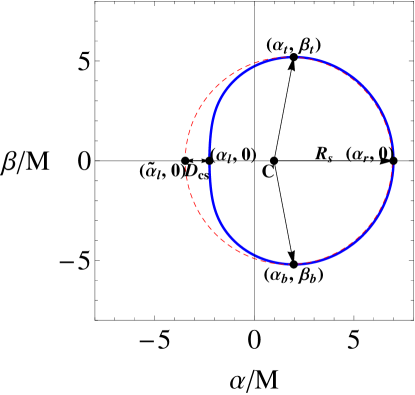
(a) Schematic illustration for Eq. (43)

(b) Kerr one with increasing $a$

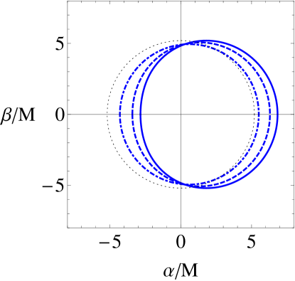
(c) Kerr one with increasing $\theta$

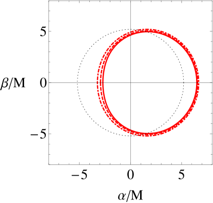
(d) Kerr-Newman one with increasing $Q$

Figure 2: (color online). Schematic illustration for observables of a black hole shadow.

Figure 2 represents schematic illustrations of a black hole shadow. The rotation direction with $a>0$ is assumed to be counterclockwise when observing from the positive $\beta$-axis. The closed asymmetric circles represent the gravitational capture cross section of photons. The asymmetry occurs because the locations of unstable orbits for corotating and counterrotating cases are different [See Fig. 1(a)]. As we mentioned in Sec. $(3)$, the number of photons passing through the left side of the black hole rotation axis is different from that through right side. Consequently, it is found that the left side of the black hole is brighter than the right side.

In Fig. 2(a), $D_{cs}$ denotes the difference between the left endpoints of the shadow and the reference circle. The subscript $t$, $r$, $l$ indicate, respectively, the coordinates of the shadow vertices at the top, right, and left endpoint, while ${\tilde{\alpha}}_{l}$ is the coordinate for the left edge of referenced circle. $R_{s}$ is the approximate shadow radius of the circle passing through three points, $\alpha_{t}$, $\alpha_{b}$, and $\alpha_{r}$. $(\alpha_{r},\alpha_{l})$ and $(\beta_{t},\beta_{b})$ represent the horizontal and vertical diameters of the shadow, respectively.

Figure 2(b) shows the shadow of Kerr black hole with increasing $a$. The grey dotted circle indicates the shadow induced by Schwarzschild black hole with $a=0$. The black dot-dashed circle shows the shadow induced by Kerr black hole with $a=0.3$, the dashed circle with $a=0.7$, the solid circle with $a=0.9$, respectively. The circle’s vertical-axis asymmetry increases and shifts to the right as $a$ increases.

Figure 2(c) implies the shadow of Kerr black hole with increasing $\theta$ with $a=0.9$. The blue dot-dashed circle shows the shadow by Kerr black hole with $\theta=17.14$, the dashed circle with $\theta=\pi/4$, the solid circle with $\theta=\pi/2$, respectively. The circle’s vertical-axis asymmetry increases and shifts to the right, as $\theta$ increases.

Figure 2(d) indicates the shadow of Kerr-Newman black hole with increasing $Q$. The red dot-dashed circle shows the shadow induced by Kerr-Newman black hole with $a=0.8$ and $Q=0$ (Kerr black hole), the dashed circle with $Q=0.4$, the solid circle with $Q=0.5$, respectively. As $Q$ increases, the circle’s vertical-axis asymmetry increases and shifts to the right, and the area decreases.

From now on, we consider the case that the observer is located in the equatorial plane $(\theta_{o}=\pi/2)$.

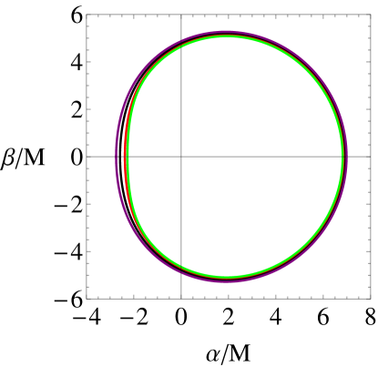
(a) $w$=3/4 and $Q$=0

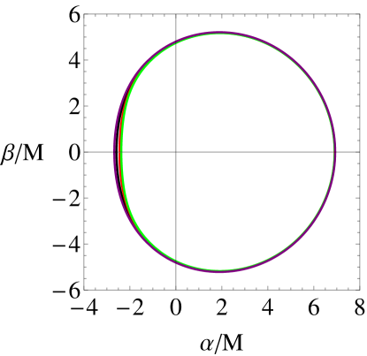
(b) $w$=6/4 and $Q$=0

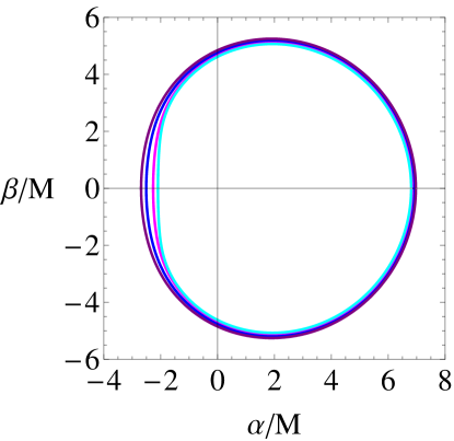
(c) $w$=3/4 and $Q$=0.15

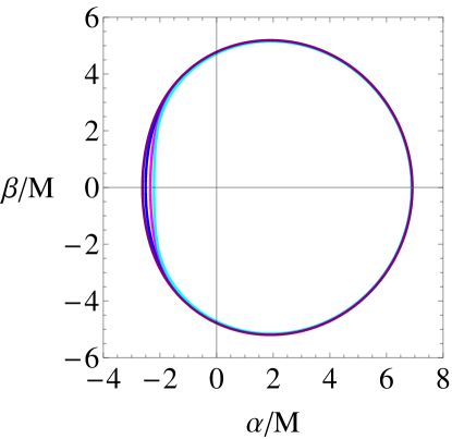
(d) $w$=6/4 and $Q$=0.15

Figure 3: (color online). Shadow casts induced by rotating black holes with anisotropic matter. (a) and (b) Kerr black hole with $Q=0$. (c) and (d) Kerr-Newman black hole with $Q=0.15$.

Figure 3 represents the shadow casts by rotating black holes with selected parameters. Figure 3(a) and (b) are shadow casts with $Q=0$, $w=3/4$ for (a) and $w=6/4$ for (b), while (c) and (d) are those with $Q=0.15$, $w=3/4$ for (c) and $w=6/4$ for (d), respectively. In Fig. 3(a) and (b), the black circles show shadow casts by Kerr black hole, the red circles show those with $K=-0.05$, the green circles show those with $K=-0.07$, and the purple circle shows those with $K=0.05$. In Fig. 3(c) and (d), the blue circles show shadow casts induced by Kerr-Newman black hole, the magenta circles show those with $K=-0.05$, the cyan circles show those with $K=-0.07$, and the purple circle shows those with $K=0.05$. The circle’s vertical-axis asymmetry increases and it shifts to the right, and the area increases as $K$ increases. The difference among the deformed circles decreases as $w$ increases. Because the positive energy condition, $Q^{2}+r^{2w}_{o}r^{2(1-w)}\geq 0$ as shown in [35], for the cases with $K=0.05$, we focus on figuring out the shadow cast depending on the negative $K$.

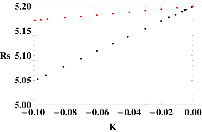
(a) Shadow radius $Q$=0

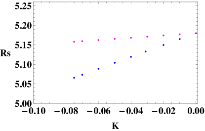
(b) Shadow radius $Q$=0.15

Figure 4: (color online). Approximate shadow radius $R_{s}$ as function of $K$.

Figure 4 represents the approximate shadow radius $R_{s}$ with respect to $K$. Figure 4(a) is the case with $a=0.95M$ and $Q=0$. The black dots denote the radius with $w=3/4$, while the red dots represent the radius with $w=6/4$. Figure 4(b) is the case with $a=0.95M$ and $Q=0.15M$. The blue dots correspond to the radius with $w=3/4$, while the magenta dots correspond to the radius with $w=6/4$. The graphs show that the approximate shadow radius $R_{s}$ increases as $K$ increases.

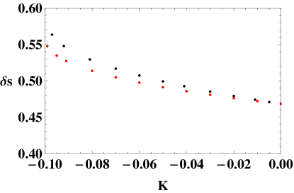
(a) Distortion parameter $Q$=0

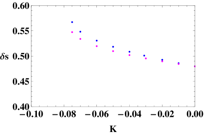
(b) Distortion parameter $Q$=0.15

Figure 5: (color online). Distortion parameter $\delta_{s}$ as function of $K$.

Figure 5 represents the distortion parameter $\delta_{s}$ versus $K$. Figure 5(a) is the case with $a=0.95M$ and $Q=0$. The black dots correspond to the distortion parameter with $w=3/4$, while the red dots correspond to the distortion parameter with $w=6/4$. Figure 5(b) is the case with $a=0.95M$ and $Q=0.15M$. The blue dots represent the distortion parameter with $w=3/4$, while the magenta dots denote the distortion parameter with $w=6/4$. These show that the distortion parameter $\delta_{s}$ decreases as $K$ increases.

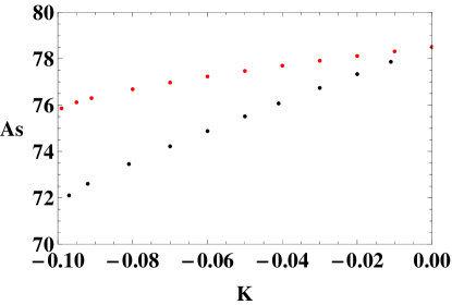
(a) Area $Q$=0

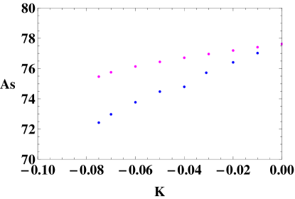
(b) Area $Q$=0.15

Figure 6: (color online). Area $A_{s}$ as function of $K$.

Figure 6 presents the area $A_{S}$ with respect to $K$. Figure 6(a) is the case with $a=0.95M$ and $Q=0$. The black dots correspond to the area with $w=3/4$, while the red dots denote the area with $w=6/4$. Figure 6(b) is the case with $a=0.95M$ and $Q=0.15M$. The blue dots correspond to the area with $w=3/4$, while the magenta dots indicate the area with $w=6/4$. The graphs show that the area of the shadow $A_{s}$ increases as $K$ increases.

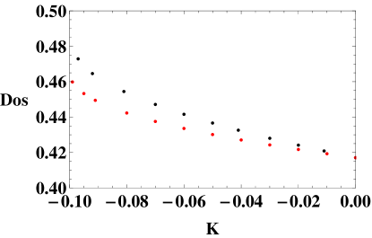
(a) Oblateness $Q$=0

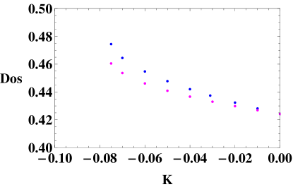
(b) Oblateness $Q$=0.15

Figure 7: (color online). Oblateness $D_{os}$ as function of $K$.

Figure 7 indicates the oblateness with respect to $K$. Figure 7(a) is the case with $a=0.95M$ and $Q=0$. The black dots correspond to the oblateness with $w=3/4$, while the red dots correspond to the oblateness with $w=6/4$. Figure 7(b) is the case with $a=0.95M$ and $Q=0.15M$. The blue dots correspond to the oblateness with $w=3/4$, while the magenta dots correspond to the oblateness with $w=6/4$. The graphs show that the oblateness $D_{os}$ decreases when $K$ increases.

5 Summary and discussions

We have investigated the shadow cast induced by a rotating black hole with an anisotropic matter field. For this study, we assumed that the matter field interacts with light rays through gravitational interaction. We first explored the symmetry of the rotating black hole geometry and its separability structure. We have found the Killing tensor explicitly, implying the separability structure and integrability of the geodesic motions.

The geodesic equations are derived by adopting the Hamilton-Jacobi formalism. We have analyzed the radial null geodesic motion for both corotating and counterrotating cases. The photon orbits for corotating cases are located inside the ergosphere, implying that some counterrotating photons can change their rotating direction. Thus, it is found that one side of the black hole is brighter than the other side. We used the backward ray-tracing algorithm to get the relation between two impact parameters and the coordinates axes in spatial infinity. The size of the black hole shadow depends on its mass mainly, while the shape depends both rotation and inclination angle. In this work, we have taken $\theta=\pi/2$, large values of $Q$ and $K$ to show the difference among parameters clearly. Also, we selected specific values $w$. We expect that densities for $Q$ and $K$ are very smaller than those for mass and rotation for a real black hole.

We have presented the shadow cast induced by rotating black holes in Fig. 3. The left side corresponds to the corotating direction between the light rays and the black hole, while the right side to the counterrotating one between the light rays and the black hole. It is observed that the left side becomes flattened when $K$ decreases. We have investigated four observables to see their dependence on parameters of a black hole. The approximate shadow radius $R_{s}$ increases as $K$ increases. The distortion parameter $\delta_{s}$ decreases as $K$ increases and $w$ has the lower value for both cases. The area of the shadow $A_{s}$ increases as $K$ increases. Lastly, the oblateness $D_{os}$ decreases as $K$ increases. If we require the positive energy condition satisfying $Q^{2}+r^{2w}_{o}r^{2(1-w)}\geq 0$ as shown in [35], there will be a small room for the positive value of $K$. Therefore, we mainly analyzed four observables with negative values of $K$, except for Fig. 3 to get the deformation behavior of the shadow cast. Our results suggest that the observed black hole mass might be either underestimated or overestimated depending on the sign of the matter field ($K$), even though the difference is very small.

According to [18], they measured emission ring diameter $d=42\pm 3\mu$as, angular size $11^{+0.5}_{-0.3}$ in units of mass, and observed inclination angle $\theta_{o}\approx 17^{\circ}$ [113, 18] for M$87^{*}$’s shadow. It suggests that the supermassive black hole (M$87^{*}$) is lying at a small angle in the direction of the observer’s line of sight. Thus, the angular size seems to be similar to that for Schwarzschild black hole. However, one knows that M$87^{*}$ rotates with an estimated rotation $a=0.90\pm 0.05$ [114]. It is worth to note that a significant difference between position angles of brightness maximum measured in $2013$ and $2017$ was found in [115]. On the other hand, there have been attempted to make an image of SgrA^∗ in the Milky Way [116, 16, 17] in the radio spectrum through very-long-baseline interferometry (VLBI) experiments [25, 117]. They estimated the emission ring diameter for the source as $d\sim 50\mu$as[118, 16, 17] and the inclination angle $\theta_{o}>30^{\circ}$ [119, 120]. It is interesting to note that SgrA^∗ has a larger inclination angle than M87^∗. Hence, one expects that its shadow cast will show an asymmetric brighter side than M$87^{*}$ and be detected with new-generation instruments.

Two research directions for the black hole shadow are known as theoretical and observational approaches. In this paper, we have focused on the theoretical aspect in light of the observation. At this stage, it is not easy to determine the parameters of the rotating black hole exactly through the shadow image. However, we hope that both the upgraded EHT and the BlackHoleCam project will detect the shadow image with a much higher resolution in the near future.

Finally, we did not consider the effect of an accretion disk at all. For this, we should construct the accretion disk [121, 122, 123, 124] in the geometry of the rotating black hole with an anisotropic matter field. This issue will be considered as an interesting subject and thus, we remain it for a future work.

References

- [1] K. Schwarzschild, Sitzungsber. Preuss. Akad. Wiss. Berlin (Math. Phys. ) 1916, 189 (1916) [physics/9905030].
- [2] J. R. Oppenheimer and H. Snyder, Phys. Rev. 56, 455 (1939).
- [3] R. P. Kerr, Phys. Rev. Lett. 11, 237 (1963).
- [4] E. T. Newman, R. Couch, K. Chinnapared, A. Exton, A. Prakash and R. Torrence, J. Math. Phys. 6, 918 (1965).
- [5] R. Penrose, Phys. Rev. Lett. 14, 57 (1965).
- [6] R. Penrose, Riv. Nuovo Cim. 1, 252 (1969) [Gen. Rel. Grav. 34, 1141 (2002)].
- [7] R. Ruffini and J. A. Wheeler, Phys. Today 24, no. 1, 30 (1971).
- [8] A. E. Broderick, R. Narayan, J. Kormendy, E. S. Perlman, M. J. Rieke and S. S. Doeleman, Astrophys. J. 805, no. 2, 179 (2015) [arXiv:1503.03873 [astro-ph.HE]].
- [9] A. Einstein, Science 84, 506 (1936).
- [10] G. Reber, Astrophys. J. 100, 279 (1944).
- [11] M. Schmidt, Nature 197, no. 4872, 1040 (1963).
- [12] R. Narayan and J. E. McClintock, arXiv:1312.6698 [astro-ph.HE].
- [13] B. P. Abbott et al. [LIGO Scientific and Virgo Collaborations], Phys. Rev. Lett. 116, no. 24, 241103 (2016) [arXiv:1606.04855 [gr-qc]].
- [14] B. P. Abbott et al. [LIGO Scientific and VIRGO Collaborations], Phys. Rev. Lett. 118, no. 22, 221101 (2017) Erratum: [Phys. Rev. Lett. 121, no. 12, 129901 (2018)] [arXiv:1706.01812 [gr-qc]].
- [15] J. Kormendy and D. Richstone, Ann. Rev. Astron. Astrophys. 33, 581 (1995).
- [16] A. M. Ghez et al., Astrophys. J. 689, 1044 (2008) [arXiv:0808.2870 [astro-ph]].
- [17] S. Gillessen, F. Eisenhauer, S. Trippe, T. Alexander, R. Genzel, F. Martins and T. Ott, Astrophys. J. 692, 1075 (2009) [arXiv:0810.4674 [astro-ph]].
- [18] K. Akiyama et al. [Event Horizon Telescope Collaboration], Astrophys. J. 875, no. 1, L1 (2019).
- [19] K. Akiyama et al. [Event Horizon Telescope Collaboration], Astrophys. J. 875, no. 1, L4 (2019).
- [20] K. Akiyama et al. [Event Horizon Telescope Collaboration], Astrophys. J. 875, no. 1, L5 (2019).
- [21] J. M. Bardeen, 1973, in Black Holes, ed. C. DeWitt and B. S. DeWitt (New York: Gordon Breach), 215-239.
- [22] C. T. Cunningham and J. M. Bardeen, Astrophys. J. 183, 237 (1973).
- [23] P. J. Young, Phys. Rev. D 14, 3281 (1976).
- [24] J.-P. Luminet, Astron. Astrophys. 75, 228 (1979).
- [25] H. Falcke, F. Melia and E. Agol, Astrophys. J. 528, L13 (2000) [astro-ph/9912263].
- [26] P. V. P. Cunha and C. A. R. Herdeiro, Gen. Rel. Grav. 50, no. 4, 42 (2018) [arXiv:1801.00860 [gr-qc]].
- [27] V. I. Dokuchaev and N. O. Nazarova, J. Exp. Theor. Phys. 128, no. 4, 578 (2019) [arXiv:1804.08030 [astro-ph.HE]].
- [28] R. Narayan, M. D. Johnson and C. F. Gammie, Astrophys. J. Lett. 885, no. 2, L33 (2019) [arXiv:1910.02957 [astro-ph.HE]].
- [29] F. Zwicky, Helv. Phys. Acta 6, 110 (1933) [Gen. Rel. Grav. 41, 207 (2009)].
- [30] V. C. Rubin and W. K. Ford, Jr., Astrophys. J. 159, 379 (1970).
- [31] N. Aghanim et al. [Planck Collaboration], Astron. Astrophys. 641, A6 (2020) [arXiv:1807.06209 [astro-ph.CO]].
- [32] S. Kang, S. Scopel and G. Tomar, Phys. Rev. D 99, no. 10, 103019 (2019) [arXiv:1902.09121 [hep-ph]].
- [33] I. Cho and H. C. Kim, Chin. Phys. C 43, no. 2, 025101 (2019) [arXiv:1703.01103 [gr-qc]].
- [34] I. Cho, Eur. Phys. J. C 79, no. 1, 42 (2019) [arXiv:1712.00577 [gr-qc]].
- [35] H. C. Kim, B. H. Lee, W. Lee and Y. Lee, Phys. Rev. D 101, no. 6, 064067 (2020) [arXiv:1912.09709 [gr-qc]].
- [36] I. G. Dymnikova, Sov. Phys. Usp. 29, 215 (1986).
- [37] A. de Vries, Class. Quant. Grav. 17, 123 (2000).
- [38] K. Hioki and K. I. Maeda, Phys. Rev. D 80, 024042 (2009) [arXiv:0904.3575 [astro-ph.HE]].
- [39] R. A. Konoplya, Phys. Lett. B 795, 1 (2019) [arXiv:1905.00064 [gr-qc]].
- [40] F. Atamurotov, B. Ahmedov, and A. Abdujabbarov, Phys. Rev. D 92, 084005 (2015) [arXiv:1507.08131 [gr-qc]].
- [41] A. A. Abdujabbarov, L. Rezzolla and B. J. Ahmedov, Mon. Not. Roy. Astron. Soc. 454, no. 3, 2423 (2015) [arXiv:1503.09054 [gr-qc]].
- [42] A. Abdujabbarov, M. Amir, B. Ahmedov and S. G. Ghosh, Phys. Rev. D 93, no. 10, 104004 (2016) [arXiv:1604.03809 [gr-qc]].
- [43] X. Hou, Z. Xu, M. Zhou and J. Wang, JCAP 1807, 015 (2018) [arXiv:1804.08110 [gr-qc]].
- [44] Z. Stuchlik, D. Charbulak and J. Schee, Eur. Phys. J. C 78, no. 3, 180 (2018) [arXiv:1811.00072 [gr-qc]].
- [45] S. Haroon, M. Jamil, K. Jusufi, K. Lin and R. B. Mann, Phys. Rev. D 99, no. 4, 044015 (2019) [arXiv:1810.04103 [gr-qc]].
- [46] K. Jusufi, M. Jamil, P. Salucci, T. Zhu and S. Haroon, Phys. Rev. D 100, no. 4, 044012 (2019) [arXiv:1905.11803 [physics.gen-ph]].
- [47] S. W. Wei, Y. C. Zou, Y. X. Liu and R. B. Mann, JCAP 1908, 030 (2019) [arXiv:1904.07710 [gr-qc]].
- [48] R. Roy and U. A. Yajnik, Phys. Lett. B 803, 135284 (2020) [arXiv:1906.03190 [gr-qc]].
- [49] S. Vagnozzi, C. Bambi and L. Visinelli, Class. Quant. Grav. 37, no. 8, 087001 (2020) [arXiv:2001.02986 [gr-qc]].
- [50] Z. Chang and Q. H. Zhu, Phys. Rev. D 101, no. 8, 084029 (2020) [arXiv:2001.05175 [gr-qc]].
- [51] J. Badia and E. F. Eiroa, Phys. Rev. D 102, no. 2, 024066 (2020) [arXiv:2005.03690 [gr-qc]].
- [52] V. I. Dokuchaev and N. O. Nazarova, Universe 6, no. 9, 154 (2020) [arXiv:2007.14121 [astro-ph.HE]].
- [53] P. Z. He, Q. Q. Fan, H. R. Zhang and J. B. Deng, Eur. Phys. J. C 80, no. 12, 1195 (2020) [arXiv:2009.06705 [gr-qc]].
- [54] M. Zhang and J. Jiang, Phys. Rev. D 103, no. 2, 025005 (2021) [arXiv:2010.12194 [gr-qc]].
- [55] A. Chowdhuri and A. Bhattacharyya, arXiv:2012.12914 [gr-qc].
- [56] P. Bambhaniya, D. Dey, A. B. Joshi, P. S. Joshi, D. N. Solanki and A. Mehta, arXiv:2101.03865 [gr-qc].
- [57] P. G. Nedkova, V. K. Tinchev and S. S. Yazadjiev, Phys. Rev. D 88, no. 12, 124019 (2013) [arXiv:1307.7647 [gr-qc]].
- [58] C. Bambi, Phys. Rev. D 87, 107501 (2013) [arXiv:1304.5691 [gr-qc]].
- [59] M. Amir, K. Jusufi, A. Banerjee and S. Hansraj, Class. Quant. Grav. 36, no. 21, 215007 (2019) [arXiv:1806.07782 [gr-qc]].
- [60] C. Bambi, K. Freese, S. Vagnozzi and L. Visinelli, Phys. Rev. D 100, no. 4, 044057 (2019) [arXiv:1904.12983 [gr-qc]].
- [61] K. Hioki and U. Miyamoto, Phys. Rev. D 78, 044007 (2008) [arXiv:0805.3146 [gr-qc]].
- [62] L. Amarilla and E. F. Eiroa, Phys. Rev. D 85, 064019 (2012) [arXiv:1112.6349 [gr-qc]].
- [63] S. W. Wei and Y. X. Liu, JCAP 1311, 063 (2013) [arXiv:1311.4251 [gr-qc]].
- [64] P. V. P. Cunha, C. A. R. Herdeiro, E. Radu and H. F. Runarsson, Phys. Rev. Lett. 115, no. 21, 211102 (2015) [arXiv:1509.00021 [gr-qc]].
- [65] Z. Younsi, A. Zhidenko, L. Rezzolla, R. Konoplya and Y. Mizuno, Phys. Rev. D 94, no. 8, 084025 (2016) [arXiv:1607.05767 [gr-qc]].
- [66] M. Sharif and S. Iftikhar, Eur. Phys. J. C 76, no. 11, 630 (2016) [arXiv:1611.00611 [gr-qc]].
- [67] R. Shaikh, Phys. Rev. D 100, no. 2, 024028 (2019) [arXiv:1904.08322 [gr-qc]].
- [68] S. Vagnozzi and L. Visinelli, Phys. Rev. D 100, no. 2, 024020 (2019) [arXiv:1905.12421 [gr-qc]].
- [69] A. Allahyari, M. Khodadi, S. Vagnozzi and D. F. Mota, JCAP 2002, 003 (2020) [arXiv:1912.08231 [gr-qc]].
- [70] R. Kumar, S. G. Ghosh and A. Wang, Phys. Rev. D 101, no. 10, 104001 (2020) [arXiv:2001.00460 [gr-qc]].
- [71] B. Eslam Panah, K. Jafarzade and S. H. Hendi, Nucl. Phys. B 961, 115269 (2020) [arXiv:2004.04058 [hep-th]].
- [72] M. Khodadi, A. Allahyari, S. Vagnozzi and D. F. Mota, JCAP 2009, 026 (2020) [arXiv:2005.05992 [gr-qc]].
- [73] F. Long, S. Chen, M. Wang and J. Jing, Eur. Phys. J. C 80, no. 12, 1180 (2020) [arXiv:2009.07508 [gr-qc]].
- [74] E. Contreras, A. Rincon, G. Panotopoulos and P. Bargueno, arXiv:2010.03734 [gr-qc].
- [75] J. Schee and Z. Stuchlik, Int. J. Mod. Phys. D 18, 983 (2009) [arXiv:0810.4445 [astro-ph]].
- [76] D. Astefanesei, C. Herdeiro, A. Pombo and E. Radu, JHEP 1910, 078 (2019) [arXiv:1905.08304 [hep-th]].
- [77] D. C. Zou and Y. S. Myung, Phys. Lett. B 803, 135332 (2020) [arXiv:1911.08062 [gr-qc]].
- [78] Y. S. Myung and D. C. Zou, Phys. Lett. B 811, 135905 (2020) [arXiv:2009.05193 [gr-qc]].
- [79] V. Frolov, P. Krtous and D. Kubiznak, Living Rev. Rel. 20, no. 1, 6 (2017) [arXiv:1705.05482 [gr-qc]].
- [80] F. H. Vincent, T. Paumard, E. Gourgoulhon and G. Perrin, Class. Quant. Grav. 28, 225011 (2011) [arXiv:1109.4769 [gr-qc]].
- [81] O. James, E. von Tunzelmann, P. Franklin and K. S. Thorne, Class. Quant. Grav. 32, no. 6, 065001 (2015) [arXiv:1502.03808 [gr-qc]].
- [82] P. V. P. Cunha, C. A. R. Herdeiro, E. Radu and H. F. Runarsson, Int. J. Mod. Phys. D 25, no. 09, 1641021 (2016) [arXiv:1605.08293 [gr-qc]].
- [83] G. W. Gibbons and S. W. Hawking, Phys. Rev. D 15, 2752 (1977).
- [84] S. W. Hawking and S. F. Ross, Phys. Rev. D 52, 5865 (1995) [hep-th/9504019].
- [85] R. Ruffini and J. A. Wheeler, PRINT-70-2077.
- [86] L. P. Eisenhart, Riemannian Geometry, Pinceton University Press, Princeton, NJ, 1949.
- [87] B. Carter, Phys. Rev. Lett. 26, 331 (1971).
- [88] M. Walker and R. Penrose, Commun. Math. Phys. 18, 265 (1970).
- [89] W. Kinnersley, J. Math. Phys. 10, 1195 (1969).
- [90] H. Kim, C. H. Lee and H. K. Lee, Phys. Rev. D 63, 064037 (2001) [gr-qc/0011044].
- [91] S. Chandrasekhar, The mathematical theory of black holes OXFORD, UK: CLARENDON (1985) 646 P.
- [92] S. Benenti and M. Francaviglia, Gen. Rel. Grav. 10, no. 1, 79 (1979).
- [93] M. Demianski and M. Francaviglia, Int. J. Theor. 19, 675 (1980).
- [94] B. Gwak, B. H. Lee and W. Lee, J. Korean Phys. Soc. 54, 2202 (2009) [arXiv:0806.4320 [gr-qc]].
- [95] B. Gwak, B. H. Lee, W. Lee and H. C. Kim, Gen. Rel. Grav. 43, 2277 (2011) [arXiv:1003.3102 [gr-qc]].
- [96] H. C. Lee and Y. J. Han, Eur. Phys. J. C 77, no. 10, 655 (2017) [arXiv:1704.02740 [gr-qc]].
- [97] C. L. A. Rizwan, A. Naveena Kumara, K. Hegde, M. S. Ali and A. K. M, arXiv:2008.01426 [gr-qc].
- [98] B. Carter, Phys. Rev. 174, 1559 (1968).
- [99] D. C. Wilkins, Phys. Rev. D 5, 814 (1972).
- [100] E. Teo, Gen. Rel. Grav. 35, 1909 (2003).
- [101] M. Zajacek, A. Tursunov, A. Eckart and S. Britzen, Mon. Not. Roy. Astron. Soc. 480, no. 4, 4408 (2018) [arXiv:1808.07327 [astro-ph.GA]].
- [102] A. Z. Petrov, Gen. Rel. Grav. 32, 1665 (2000).
- [103] F. A. E. Pirani, Phys. Rev. 105, 1089 (1957).
- [104] R. Penrose, Annals Phys. 10, 171 (1960).
- [105] C. W. Misner, K. S. Thorne and J. A. Wheeler, San Francisco 1973, 1279p
- [106] D. Psaltis and T. Johannsen, Astrophys. J. 745, 1 (2012) [arXiv:1011.4078 [astro-ph.HE]].
- [107] J. M. Bardeen, W. H. Press and S. A. Teukolsky, Astrophys. J. 178, 347 (1972).
- [108] V. P. Frolov and I. D. Novikov, Black hole physics: Basic concepts and new developments, Fundam. Theor. Phys. 96 (1998).
- [109] S. E. Vazquez and E. P. Esteban, Nuovo Cim. B 119, 489 (2004) [gr-qc/0308023].
- [110] R. Takahashi, J. Korean Phys. Soc. 45, S1808 (2004) [Astrophys. J. 611, 996 (2004)] [astro-ph/0405099].
- [111] O. Y. Tsupko, Phys. Rev. D 95, no. 10, 104058 (2017) [arXiv:1702.04005 [gr-qc]].
- [112] R. Kumar and S. G. Ghosh, Astrophys. J. 892, 78 (2020) [arXiv:1811.01260 [gr-qc]].
- [113] R. Craig Walker, P. E. Hardee, F. B. Davies, C. Ly and W. Junor, Astrophys. J. 855, no. 2, 128 (2018) [arXiv:1802.06166 [astro-ph.HE]].
- [114] F. Tamburini, B. Thide and M. Della Valle, Mon. Not. Roy. Astron. Soc. 492, no. 1, L22 (2020) [arXiv:1904.07923 [astro-ph.HE]].
- [115] M. Wielgus et al. [Event Horizon Telescope Collaboration], Astrophys. J. 901, no. 1, 67 (2020) [arXiv:2009.11842 [astro-ph.HE]].
- [116] B. Balick and R. L. Brown, Astrophys. J. 194, 265 (1974).
- [117] C. Goddi et al., Int. J. Mod. Phys. D 26, no. 02, 1730001 (2017) [arXiv:1606.08879 [astro-ph.HE]].
- [118] R. S. Lu et al., Astrophys. J. 859, no. 1, 60 (2018) [arXiv:1805.09223 [astro-ph.GA]].
- [119] A. E. Broderick, V. L. Fish, S. S. Doeleman and A. Loeb, Astrophys. J. 697, 45 (2009) [arXiv:0809.4490 [astro-ph]].
- [120] M. J. Reid et al., Astrophys. J. 783, 130 (2014) [arXiv:1401.5377 [astro-ph.GA]].
- [121] I. D. Novikov and K. S. Thorne, in Black Holes, edited by C. DeWitt and B. S. DeWitt (Gordon Breach, New York, 1973), pp. 343-550.
- [122] D. N. Page and K. S. Thorne, Astrophys. J. 191, 499 (1974).
- [123] U. Jang, Y. Yi and H. Kim, arXiv:2002.10885 [astro-ph.HE].
- [124] L. G. Collodel, D. D. Doneva and S. S. Yazadjiev, arXiv:2101.05073 [astro-ph.HE].