Energy-Efficient Distributed Learning Algorithms for Coarsely Quantized Signals

Abstract

In this work, we present an energy-efficient distributed learning framework using low-resolution ADCs and coarsely quantized signals for Internet of Things (IoT) networks. In particular, we develop a distributed quantization-aware least-mean square (DQA-LMS) algorithm that can learn parameters in an energy-efficient fashion using signals quantized with few bits while requiring a low computational cost. We also carry out a statistical analysis of the proposed DQA-LMS algorithm that includes a stability condition. Simulations assess the DQA-LMS algorithm against existing techniques for a distributed parameter estimation task where IoT devices operate in a peer-to-peer mode and demonstrate the effectiveness of the DQA-LMS algorithm.

I Introduction

Distributed signal processing algorithms are of great relevance for statistical inference in wireless networks and applications such as wireless sensor networks (WSNs) [1] and the Internet of Things (IoT) [2]. These techniques deal with the extraction of information from data collected at nodes that are distributed over a geographic area. Prior work on distributed approaches has studied protocols for exchanging information [3, 4, 5], adaptive learning algorithms [6, 7, 8, 9], the exploitation of sparse and low-rank measurements [10, 11, 12], topology adaptation [13], compensation methods for highly correlated input signals [14], and robust techniques against interference and noise [15]. Although there are many studies on the need for data exchange and signaling among nodes as well as their complexity, prior work on energy-efficient techniques is rather limited.

In this context, energy-efficient signal processing techniques have gained a great deal of interest in the last decade or so due to their ability to save energy and promote sustainable development of electronic systems and devices. Electronic devices often exhibit a power consumption that is dependent on the communication module [16, 17] and from a circuit perspective on analog-to-digital converters (ADCs) and decoders [18]. Reducing the number of bits used to represent digital samples can greatly decrease the energy consumption by ADCs [19]. This is key to devices that are battery operated and wireless networks that must keep the power consumption to a low level for sustainability reasons. In particular, prior work on energy efficiency has reported many contributions in signal processing for communications and electronic systems that operate with coarsely quantized signals [20, 21, 22, 23, 24, 25, 26, 27].

In this work, we propose an energy-efficient distributed learning framework using low-resolution ADCs and coarsely quantized signals for IoT networks [28]. In particular, we devise a distributed quantization-aware least-mean square (DQA-LMS) algorithm that can learn parameters in an energy-efficient way using signals quantized using few bits with a low computational cost. We also develop a statistical analysis of the DQA-LMS algorithm that includes a stability condition. Simulations assess the DQA-LMS algorithm against existing techniques for a distributed parameter estimation task with IoT devices.

This paper is structured as follows: Section II introduces the signal model and states the problem. Section III details the proposed DQA-LMS algorithm, whereas Section IV analyzes DQA-LMS. Section V shows and discusses the simulation results and Section VI draws the conclusions of this work.

II Signal Model and Problem Statement

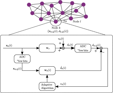
Figure 1: A distributed adaptive IoT network

We consider an IoT network consisting of $N$ nodes or agents, which run distributed signal processing techniques to perform the desired tasks, as depicted in Fig. 1. The model adopted considers a desired signal $d_{k}(i)$, at each time $i$, described by

$$d_{k}(i)={\mathbf{w}}_{o}^{H}{\mathbf{x}}_{k}(i)+v_{k}(i),\quad k=1,2,\dots,N,$$ (1)

where ${\mathbf{w}}_{o}\in\mathbb{C}^{M\times 1}$ is the parameter vector that the agents must estimate, ${\mathbf{x}}_{k}(i)\in\mathbb{C}^{M\times 1}$ is the regressor and $v_{k}(i)$ represents Gaussian noise with zero mean and variance $\sigma_{v,k}^{2}$ at node $k$. We adopt the Adapt-then-Combine (ATC) diffusion rule as it outperforms the incremental and consensus protocols [3, 4]. At each node $k$ and time $i$, based on the local data {$d_{k}(i)$, ${\mathbf{x}}_{k}(i)$} and the estimated parameter vectors ${\mathbf{h}}_{l}(i)$ from its neighborhood, the parameter vector with local estimates ${\mathbf{w}}_{k}(i)$ is updated. The ATC distributed LMS (DLMS) algorithm consists of the recursions:

$${\mathbf{h}}_{k}(i)= {\mathbf{w}}_{k}(i-1)+\mu_{k}{\mathbf{x}}_{k}(i)e_{k}^{*}(i), {\mathbf{w}}_{k}(i)= \sum_{l\in\mathcal{N}_{k}}a_{lk}{\mathbf{h}}_{l}(i),$$

where ${\mathbf{h}}_{k}(i)$ and ${\mathbf{w}}_{k}(i)$ contain the intermediate and the local estimates of ${\mathbf{w}}_{o}$ at node $k$ and time $i$, respectively, $e_{k}(i)=d_{k}(i)-\hat{d}_{k}(i)=d_{k}(i)-{\mathbf{w}}_{k}^{H}(i-1){\mathbf{x}}_{k}(i)$ is the error between the output of the adaptive filter, $\hat{d}_{k}(i)$, and the desired signal, $d_{k}(i)$, at time $i$, $\mu_{k}$ is the step-size for node $k$, $\mathcal{N}_{k}$ is the set of neighbor nodes connected to node $k$, and $a_{lk}$ are the combination coefficients of neighbor nodes at node $k$ such that

$$a_{lk}=0\,~{}{\rm if}\,l\notin\mathcal{N}_{k},~{}a_{lk}>0\,~{}{\rm if}\,l\in\mathcal{N}_{k},~{}{\rm and}\sum_{l\in{\mathcal{N}_{k}}}{a_{lk}}=1.$$ (2)

As shown in Fig. 1, as the measurement data at each node and the unknown system are analog and each agent processes local data {$d_{k}(i)$, ${\mathbf{x}}_{k}(i)$} digitally, we need two ADCs in each agent. One concern is that as the number of agents increases, the power consumption will grow considerably when using high-resolution ADCs for each agent. This motivates us to quantize signals using few bits. Therefore, the problem we are interested in solving is how to design energy-efficient distributed learning algorithms that can cost-effectively operate with coarsely quantized signals.

III Proposed DQA-LMS Algorithm

Let ${\mathbf{x}}_{k,Q}=Q_{b}({\mathbf{x}}_{k})$ denote the $b$-bit quantized output of an ADC at node $k$, described by a set of $2^{b}+1$ thresholds ${\cal T}_{b}=\{\tau_{0},\tau_{1},...,\tau_{2^{b}}\}$, such that $-\infty=\tau_{0}<\tau_{1}<...<\tau_{2^{b}}=\infty$, and the set of $2^{b}$ labels ${\cal L}_{b}=\{l_{0},l_{1},...,l_{2^{b}-1}\}$ where $l_{p}\in(\tau_{p},\tau_{p+1}]$, for $p\in[0,2^{b}-1]$ [21]. Let us assume that ${\mathbf{x}}_{k}\sim\mathcal{CN}({\mathbf{0}},\,{\mathbf{R}}_{x_{k}})$, where ${\mathbf{R}}_{x_{k}}\in\mathbb{C}^{M\times M}$ is the covariance matrix of ${\mathbf{x}}_{k}$. We now use Bussgang’s theorem [29] to derive a model for the quantized vector ${\mathbf{x}}_{k,Q}$, which we will use later to derive our DQA-LMS algorithm. Employing Bussgang’s theorem, ${\mathbf{x}}_{k,Q}$ can be decomposed as

$${\mathbf{x}}_{k,Q}={\mathbf{G}}_{k,b}{\mathbf{x}}_{k}+{\mathbf{q}}_{k},\vspace{-0.25em}\vspace{-0.25em}$$ (3)

where the quantization distortion ${\mathbf{q}}_{k}$ is uncorrelated with ${\mathbf{x}}_{k}$, and ${\mathbf{G}}_{k,b}\in\mathbb{R}^{M\times M}$ is a diagonal matrix described by

$$\begin{split}\vspace{-0.25em}{\mathbf{G}}_{k,b}={\rm diag}({\mathbf{R}}_{x_{k}})^{-\frac{1}{2}}\sum_{j=0}^{2^{b}-1}&\frac{l_{j}}{\sqrt{\pi}}\left[\exp(-\tau_{j}^{2}{\rm diag}({\mathbf{R}}_{x_{k}})^{-1})\right.\\ &\left.-\exp(-\tau_{j+1}^{2}{\rm diag}({\mathbf{R}}_{x_{k}})^{-1})\right].\end{split}$$ (4)

Note that this signal decomposition is also applied to the desired signal, $d_{k,Q}$, which is the output of the second ADC in the system, and for the particular case that ${\mathbf{R}}_{x_{k}}=\mathbb{E}[{\mathbf{x}}_{k}{\mathbf{x}}_{k}^{H}]=\sigma_{x,k}^{2}{\mathbf{I}}_{M}$, ${\mathbf{G}}_{k,b}$ becomes $g_{k,b}{\mathbf{I}}_{M}$. However, to minimize the mean square error (MSE) between ${\mathbf{x}}_{k}$ and ${\mathbf{x}}_{k,Q}$, we need to characterize the probability density function (PDF) of ${\mathbf{x}}_{k}$ to find the optimal quantization labels. Since the choice of labels based on the PDF is not practical, we assume the regressor ${\mathbf{x}}_{k}(i)$ is Gaussian, adapt the approach in [21] and approximate the thresholds and labels as follows:

1. We generate an auxiliary Gaussian random variable with unit variance and then use the Lloyd-Max algorithm [30], [31] to find a set of thresholds ${\cal{\widetilde{T}}}_{b}=\{\tau_{1},\dots,\tau_{2^{b}-1}\}$ and labels ${\cal{\widetilde{L}}}_{b}=\{\widetilde{l}_{0},\dots,\widetilde{l}_{2^{b}-1}\}$ that minimize the MSE between the unquantized and the quantized signals.

2. We complete the set of thresholds ${\cal T}_{b}$ by adding $\tau_{0}=-\infty$ and $\tau_{2^{b}}=\infty$ to the set ${\cal{\widetilde{T}}}_{b}$.

3. We rescale the labels such that the variance of the auxiliary random variable is 1. To do this, we multiply each label in the set ${\cal{\widetilde{L}}}_{b}$ by

   $$\alpha=\Big{(}2\sum\limits_{j=0}^{2^{b}-1}\tilde{l}_{j}^{2}(\Phi(\sqrt{2\tau_{j+1}^{2}})-\Phi(\sqrt{2\tau_{j}^{2}})\Big{)}^{-1/2}\vspace{-0.75em}$$ (5)

   to produce a set of suboptimal labels ${\cal L}_{b}=\alpha{\cal{\widetilde{L}}}_{b}$ , where $\Phi(.)$ is the cumulative distribution function (CDF) of a standard Gaussian random variable.

We generate these thresholds and labels offline to build ${\mathbf{G}}_{k,b}$ for the proposed DQA-LMS algorithm in what follows.

III-A Derivation of DQA-LMS

We consider ${\mathbf{x}}_{k}(t)$ and $d_{k}(t)$ as the analog input and output of the unknown system ${\mathbf{w}}_{o}$ at node $k$. Let ${\mathbf{x}}_{k}(i)$ and $d_{k}(i)$ denote the high-precision sampled versions of ${\mathbf{x}}_{k}(t)$ and $d_{k}(t)$, and ${\mathbf{x}}_{k,Q}(i)$ and $d_{k,Q}(i)$ denote the coarsely quantized versions of ${\mathbf{x}}_{k}(i)$ and $d_{k}(i)$, respectively. We assume that the input signal at each node is Gaussian with zero mean and covariance matrix ${\mathbf{R}}_{x_{k}}=E[{\mathbf{x}}_{k}{\mathbf{x}}_{k}^{H}]=\sigma_{x,k}^{2}{\mathbf{I}}_{M}$ for $k=1,2,...,N$. Using (3), we can decompose ${\mathbf{x}}_{k,Q}(i)$ and $d_{k,Q}(i)$ as

$${\mathbf{x}}_{k,Q}(i)=g_{k,b}(i){\mathbf{x}}_{k}(i)+{\mathbf{q}}_{x,k}(i),$$ (6)

$$\begin{split}d_{k,Q}(i)&=Q(d_{k}(i))\approx g_{k,b}(i)d_{k}(i)+q_{k}(i)\\ \qquad&=g_{k,b}(i){\mathbf{w}}_{o}^{H}{\mathbf{x}}_{k}(i)+\hat{q}_{k}(i),\end{split}$$ (7)

where $\hat{q}_{k}(i)=g_{k,b}(i)v_{k}(i)+q_{k}(i)$ and $g_{k,b}(i)$ are built from an estimate of ${\mathbf{R}}_{x_{k}}$ given by $\widehat{{\mathbf{R}}}_{x_{k}}={\mathbf{x}}_{k}{\mathbf{x}}_{k}^{H}$ [32] that depends on the choice of ${\mathbf{x}}_{k}$ due to (1). Because the adaptive algorithm receives a quantized signal, ${\mathbf{x}}_{k,Q}$, and the signal is assumed to be wide-sense stationary, at each time instant, we estimate $\sigma_{x,k}^{2}$ using the variance of the received input, $\sigma_{x_{k,Q}}^{2}$ and the distortion factor of the $b$-bit quantization, $\rho_{k,b}$, such that $\sigma_{x,k}^{2}\approx\sigma_{x_{k,Q}}^{2}+\rho_{k,b}$, where $\rho_{k,b}\approx\frac{\pi\sqrt{3}}{2}2^{-2b}$ [22] for a Gaussian signal using non-uniform quantization to obtain the scalar $g_{k,b}(i)$.

We show next that a learning algorithm based directly on (7) is biased for estimating $\mathbf{w}_{o}$, and show how to correct for this bias. For this, let $\beta_{k}(i)$ be a coefficient to be chosen shortly, and define $\hat{d}_{k}(i)=\beta_{k}(i){\mathbf{w}}_{k}^{H}(i-1){\mathbf{x}}_{k,Q}(i)$ and construct an MSE cost function as described by

$$\begin{split}J_{k}({\mathbf{w}}_{k}(i))&=\mathbb{E}[|e_{k,Q}(i)|^{2}]=\mathbb{E}[|d_{k,Q}(i)-\hat{d}_{k}(i)|^{2}]\\ &=\mathbb{E}[|d_{k,Q}(i)-\beta_{k}(i){\mathbf{w}}_{k}^{H}(i-1){\mathbf{x}}_{k,Q}(i)|^{2}],\end{split}$$ (8)

which depends only on the observed quantized quantities $d_{k,Q}(i)$ and $\mathbf{x}_{k,Q}(i)$. For $\beta_{k}(i)=1$ as in DLMS, the quantization of $d_{k}(i)$ would result in biased estimates of $\mathbf{w}_{o}$. In the following we show how to optimally choose $\beta_{k}(i)$ to reduce the bias. The proposed gradient-descent recursion to perform distributed learning based on (8) is described by

$${\mathbf{h}}_{k}(i)={\mathbf{w}}_{k}(i-1)-\mu_{k}\nabla J_{k}({\mathbf{w}}_{k}(i-1)).$$ (9)

To compute the gradient of (9), we write the error in (8) as

$$\begin{split}e_{k,Q}(i)&=d_{k,Q}(i)-\beta_{k}(i){\mathbf{w}}_{k}^{H}(i-1){\mathbf{x}}_{k,Q}(i)\\ &=g_{k,b}(i){\mathbf{w}}_{o}^{H}{\mathbf{x}}_{k}(i)+\hat{q}_{k}(i)-\beta_{k}(i){\mathbf{w}}_{k}^{H}(i-1)\\ &\qquad(g_{k,b}(i){\mathbf{x}}_{k}(i)+{\mathbf{q}}_{x,k}(i))\\ &=g_{k,b}(i)({\mathbf{w}}_{o}^{H}-\beta_{k}(i){\mathbf{w}}_{k}^{H}(i-1)){\mathbf{x}}_{k}(i)\\ &\qquad-\beta_{k}(i){\mathbf{w}}_{k}^{H}(i-1){\mathbf{q}}_{x,k}(i)+\hat{q}_{k}(i).\end{split}$$ (10)

We assume that ${\mathbf{R}}_{x_{k}}=\mathbb{E}[{\mathbf{x}}_{k}{\mathbf{x}}_{k}^{H}]=\sigma_{x,k}^{2}{\mathbf{I}}_{M}$ and ${\mathbf{R}}_{q,k}=\mathbb{E}[{\mathbf{q}}_{x,k}{\mathbf{q}}_{x,k}^{H}]=\sigma_{q,k}^{2}{\mathbf{I}}_{M}$. Substituting (10) in (8) and taking the expected value of (9), we have

$$\begin{split}\mathbb{E}[{\mathbf{h}}_{k}(i)]=&[{\mathbf{I}}_{M}-\mu_{k}g_{k,b}^{2}(i)\beta_{k}(i){\mathbf{R}}_{x_{k}}-\mu_{k}g_{k,b}(i)\beta_{k}(i){\mathbf{R}}_{q,k}]\\ &\cdot\mathbb{E}[{\mathbf{w}}_{k}(i-1)]+\mu g_{k,b}^{2}(i){\mathbf{R}}_{x_{k}}{\mathbf{w}}_{o}^{H}.\end{split}$$ (11)

Substituting the values of $\mathbf{R}_{x_{k}}$ and $\mathbf{R}_{q,k}$ and taking the limit on (11), we obtain

$$\lim_{i\to+\infty}\mathbb{E}[{\mathbf{h}}_{k}(i)]=\frac{1}{\beta_{k}(i)}\frac{g_{k,b}(i)\sigma_{x,k}^{2}}{g_{k,b}(i)\sigma_{x,k}^{2}+\sigma_{q,k}^{2}}{\mathbf{w}}_{o}.$$ (12)

We conclude that the solution is unbiased if we choose

$$\beta_{k}(i)=\frac{g_{k,b}(i)\sigma_{x,k}^{2}}{g_{k,b}(i)\sigma_{x,k}^{2}+\sigma_{q,k}^{2}}.$$ (13)

The gradient of $|e_{k,Q}(i)|^{2}$ with respect to ${\mathbf{w}}_{k}^{H}$ is $\nabla J_{k}({\mathbf{w}}_{k}(i-1))=-\frac{g_{k,b}(i)\sigma_{x,k}^{2}}{g_{k,b}(i)\sigma_{x,k}^{2}+\sigma_{q,k}^{2}}{\mathbf{x}}_{k,Q}(i)e_{k,Q}^{*}(i)$. After organizing the terms of the gradient, we obtain the DQA-LMS algorithm:

$$\begin{split}{\mathbf{h}}_{k}(i)&={\mathbf{w}}_{k}(i-1)+\mu_{k}\frac{g_{k,b}(i)\sigma_{x,k}^{2}}{g_{k,b}(i)\sigma_{x,k}^{2}+\sigma_{q,k}^{2}}{\mathbf{x}}_{k,Q}(i)e_{k,Q}^{*}(i),\\ {\mathbf{w}}_{k}(i)&=\sum_{l\in\mathcal{N}_{k}}a_{lk}{\mathbf{h}}_{l}(i),\vspace{-0.5em}\end{split}$$ (14)

$$\begin{split}\vspace{-0.5em}&e_{k,Q}(i)=d_{k,Q}(i)-\frac{g_{k,b}(i)\sigma_{x,k}^{2}}{g_{k,b}(i)\sigma_{x,k}^{2}+\sigma_{q,k}^{2}}{\mathbf{w}}_{k}^{H}(i-1){\mathbf{x}}_{k,Q}(i)\,,\\ &g_{k,b}(i)=\frac{1}{\sqrt{\sigma_{x_{k}}^{2}}}\sum\limits_{j=0}^{2^{b}-1}\frac{l_{j}}{\sqrt{\pi}}[\exp(\frac{-\tau_{j}^{2}}{\sigma_{x_{k}}^{2}})-\exp(\frac{-\tau_{j+1}^{2}}{\sigma_{x_{k}}^{2}})],\,\end{split}$$ (15)

and $\sigma_{x,k}^{2}\approx\sigma_{x_{k,Q}}^{2}+\rho_{k,b}$. The scalar $g_{k,b}$ can be computed offline when ${\mathbf{R}}_{x,k}$ is known and wide-sense stationary and must be estimated online when ${\mathbf{R}}_{x,k}$ is unknown or non-stationary.

III-B Computational Complexity and Energy Consumption

Table I shows the computational complexity of the DQA-LMS algorithm in terms of the number of multiplications and additions at node $k$ per time instant, where $n_{k}$ is the number of neighbor nodes connected to node $k$. At each time instant, DQA-LMS performs a few more operations ($\approx O(2^{b})$) than DLMS. Note that we compute $g_{k,b}(i)$ online since this is more appropriate for non-stationary input data. However, one can compute ${\mathbf{G}}_{k,b}$ offline if an estimate of ${\mathbf{R}}_{x_{k}}$ in (4) is available.

However, the extra complexity of DQA-LMS allows the system to work in a more energy-efficient way. In order to assess the power savings by low resolution quantization, we consider a network with $N$ nodes in which each node uses two ADCs. The power consumption of each ADC is $P_{ADC}(b)=cB2^{b}$ [33], where $B$ is the bandwidth (related to the sampling rate), $b$ is the number of quantization bits of the ADC, and $c$ is the power consumption per conversion step. Therefore, the total power consumption of the ADCs in the network is

$$P_{ADC,T}(b)=2NcB2^{b}\qquad({\rm watts}).$$ (16)

Fig. 2 shows an example of the total power consumption of ADCs in a narrowband IoT (NB-IoT) network running diffusion adaptation consisting of 20 nodes with bandwidth $B=200\,{\rm kHz}$ [34] and considering the power consumption per conversion step of each ADC, $c=494~{}{\rm fJ}$, as in [35].

TABLE I: Computational Complexity per Time Instant

Task	Multiplications	Additions	Divisions	Exponentiations
$g_{k,b}(i)=\frac{1}{\sqrt{\sigma_{x_{k}}^{2}}}\sum\limits_{j=0}^{2^{b}-1}\frac{l_{j}}{\sqrt{\pi}}[\exp(\frac{-\tau_{j}^{2}}{\sigma_{x_{k}}^{2}})-\exp(\frac{-\tau_{j+1}^{2}}{\sigma_{x_{k}}^{2}})]$	$2^{b+1}+1$	$2^{b}-1$	$2^{b}+1$	$2^{b}$
$\beta_{k}(i)=\frac{g_{k,b}(i)\sigma_{x,k}^{2}}{g_{k,b}(i)\sigma_{x,k}^{2}+\sigma_{q,k}^{2}}$	$2$	$1$	$1$	$0$
$\hat{d}_{k,Q}(i)=\beta_{k}(i){\mathbf{w}}_{k}^{H}(i){\mathbf{x}}_{k,Q}(i)$	$M+1$	$M-1$	$0$	$0$
$e_{k,Q}(i)=d_{k,Q}(i)-\hat{d}_{k,Q}(i)$	$0$	$1$	$0$	$0$
${\mathbf{h}}_{k}(i+1)={\mathbf{w}}_{k}(i)+\mu_{k}\beta_{k}(i)e_{k,Q}^{*}(i){\mathbf{x}}_{k,Q}(i)$	$M+2$	$M$	$0$	$0$
${\mathbf{w}}_{k}(i+1)=\sum\limits_{l\in\mathcal{N}_{k}}a_{lk}{\mathbf{h}}_{l}(i+1)$	$n_{k}M$	$n_{k}M$	$0$	$0$
Total (at node $k$)	$(2+n_{k})M+2^{b+1}+6$	$(2+n_{k})M+2^{b}$	$2^{b}+2$	$2^{b}$

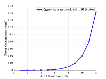
Figure 2: Power consumption of the ADCs in an adaptive IoT network.

IV Analysis of DQA-LMS

In this section, we find sufficient conditions for all local estimates to converge in the mean to the unknown parameter vector ${\mathbf{w}}_{o}$ by using the evolution of the weight error vectors [4]. Let us consider the global quantities of the network: ${\mathbf{W}}_{o}\triangleq[{\mathbf{w}}_{o},\dots,{\mathbf{w}}_{o}]_{(NM\times 1)}$, ${\mathbf{d}}_{Q}(i)\triangleq[d_{1,Q}(i),\dots,d_{N,Q}(i)]^{T}$, ${\mathbf{v}}_{i}\triangleq[v_{1}(i),\dots,v_{N}(i)]^{T}$, ${\mathbf{X}}_{Q}(i)\triangleq{\rm diag}[{\mathbf{x}}_{1,Q}^{T}(i),\dots,{\mathbf{x}}_{N,Q}^{T}(i)]$.

Using these quantities, the global form of (1) is given by ${\mathbf{d}}_{Q}(i)={\mathbf{W}}_{o}^{H}{\mathbf{X}}_{Q}(i)+{\mathbf{v}}(i)$.Defining $\mathbf{B}(i)$, $\mathbf{W}(i)$ and $\mathbf{H}(i)$ as the global quantities for, respectively, $\beta_{k}(i)$, $\mathbf{h}_{k}(i)$ and $\mathbf{w}_{k}(i)$, we can express (14) as

$$\begin{split}{\mathbf{H}}(i)&={\mathbf{W}}(i-1)+{\mathbf{D}}{\mathbf{B}}(i){\mathbf{X}}_{Q}(i)({\mathbf{d}}_{Q}(i)\\ &-{\mathbf{B}}(i){\mathbf{W}}^{H}(i-1){\mathbf{X}}_{Q}(i))^{*},\quad{\mathbf{W}}(i)={\mathbf{C}}{\mathbf{H}}(i),\end{split}$$ (17)

which can be written in a compact form as

$$\begin{split}{\mathbf{W}}(i)&={\mathbf{C}}{\mathbf{W}}(i-1)+{\mathbf{C}}{\mathbf{D}}{\mathbf{B}}(i){\mathbf{X}}_{Q}(i)({\mathbf{d}}_{Q}(i)\\ &-{\mathbf{B}}(i){\mathbf{W}}^{H}(i-1){\mathbf{X}}_{Q}(i))^{*},\end{split}$$ (18)

where ${\mathbf{D}}\triangleq{\rm diag}\{\mu_{1}I_{M},\dots,\mu_{N}I_{M}\}$ and ${\mathbf{C}}$ is an $MN\times MN$ matrix based on the combination coefficients, $a_{lk}$, defined as

$${\mathbf{A}} \triangleq\begin{bmatrix}a_{ij}\end{bmatrix}, {\mathbf{C}} \triangleq{\mathbf{A}}\otimes{\mathbf{I}}_{M}.\vspace{-0.25em}$$ (19)

Using the independence assumption [4] that states that ${\mathbf{x}}_{k,Q}(i)$ and $v_{k}(i)$ are i.i.d. in time and space with $\sigma_{v,k}^{2}=\mathbb{E}[|v_{k}(i)|^{2}]$, and $v_{k}(i)$ is independent of ${\mathbf{x}}_{k,Q}(i)$, we define the weight error vector, $\widetilde{{\mathbf{w}}}_{k}(i)$ and its global vector $\widetilde{{\mathbf{w}}}(i)$ as

$$\widetilde{{\mathbf{W}}}(i)\triangleq{\mathbf{W}}_{o}-{\mathbf{W}}(i).\vspace{-0.25em}$$ (20)

Note that using diffusion combination policies for $a_{lk}$, we have ${\mathbf{C}}{\mathbf{W}}_{o}={\mathbf{W}}_{o}$ [4]. Subtracting ${\mathbf{W}}_{o}$ from the left-hand side and ${\mathbf{C}}{\mathbf{W}}_{o}$ from the right-hand side of (18), we have

$$\begin{split}\vspace{-0.25em}\widetilde{{\mathbf{W}}}(i)&={\mathbf{C}}{\mathbf{W}}_{o}-{\mathbf{C}}{\mathbf{W}}(i-1)-{\mathbf{C}}{\mathbf{D}}{\mathbf{B}}(i){\mathbf{X}}_{Q}(i)\\ &={\mathbf{C}}\widetilde{{\mathbf{W}}}(i-1)-{\mathbf{C}}{\mathbf{D}}{\mathbf{B}}(i){\mathbf{X}}_{Q}(i)\\ &\qquad({\mathbf{X}}_{Q}^{*}(i){\mathbf{B}}(i)^{*}\widetilde{{\mathbf{W}}}(i-1)+{\mathbf{v}}^{*}(i))\\ &={\mathbf{C}}({\mathbf{I}}_{MN}-{\mathbf{D}}{\mathbf{B}}(i){\mathbf{X}}_{Q}(i){\mathbf{X}}_{Q}^{*}(i){\mathbf{B}}(i)^{*})\widetilde{{\mathbf{W}}}(i-1)\\ &\qquad-{\mathbf{C}}{\mathbf{D}}{\mathbf{B}}(i){\mathbf{X}}_{Q}(i){\mathbf{v}}^{*}(i).\end{split}$$ (21)

Taking the expectation of both sides of (21), we have

$$\mathbb{E}[\widetilde{{\mathbf{W}}}(i)]=C({\mathbf{I}}_{MN}-{\mathbf{D}}{\mathbf{R}}_{Q})\mathbb{E}[\widetilde{{\mathbf{W}}}(i-1)],$$ (22)

where $C\triangleq\mathbb{E}[{\mathbf{C}}]$, ${\mathbf{R}}_{Q}\triangleq{\rm diag}\{{\mathbf{R}}_{1,Q},\dots,{\mathbf{R}}_{N,Q}\}$ and ${\mathbf{R}}_{k,Q}=\mathbb{E}[{\mathbf{B}}_{k}(i){\mathbf{x}}_{k,Q}(i){\mathbf{x}}_{k,Q}^{*}(i){\mathbf{B}}_{k}(i)^{*}]$.

To ensure stability of the recursion in (22) with the independence assumption and using combinations that satisfy (2), there exist sufficiently small step-sizes $\mu_{k}<\mu_{max}$ such that

$$\|\mathbb{E}[\widetilde{{\mathbf{W}}}(i)]\|_{bl_{\infty}}\leq\|C\|_{bl_{\infty}}.\|{\mathbf{E}}_{i}\|_{bl_{\infty}}.\|\mathbb{E}[\widetilde{{\mathbf{w}}}(i-1)]\|_{bl_{\infty}},$$ (23)

where $\|.\|_{bl_{\infty}}$ denotes the block maximum norm [36] and ${\mathbf{E}}_{i}={\mathbf{I}}_{MN}-{\mathbf{D}}{\mathbf{R}}_{Q}$. In order for DQA-LMS to converge, we hold (23) such that $\|{\mathbf{E}}\|_{bl_{\infty}}<1$ and $\|C_{i}\|_{bl_{\infty}}\leq 1$ for all $i\geq 0$. It is proven in [36] that possibly random, time-varying convex combinations generated by ATC or CTA diffusion algorithms ensure $\|C_{i}\|_{bl_{\infty}}\leq 1$. Therefore, to find sufficient conditions on step-sizes, we must have ${\mathbf{I}}_{MN}-{\mathbf{D}}{\mathbf{R}}_{Q}<1$.

We now employ the eigenvalue decomposition ${\mathbf{R}}_{k,Q}={\mathbf{\Phi}}_{k,Q}{\mathbf{\Lambda}}_{k,Q}{\mathbf{\Phi}}_{k,Q}^{H}$, where ${\mathbf{\Lambda}}_{k,Q}$ is an $M\times M$ diagonal matrix consisting of the eigenvalues $\{\lambda_{(k,Q)_{1}},\dots,\lambda_{(k,Q)_{M}}\}$ of ${\mathbf{R}}_{k,Q}$, and the matrix ${\mathbf{\Phi}}_{k,Q}$ is an $M\times M$ square matrix whose columns are the eigenvectors $\{\boldsymbol{\phi}_{(k,Q)_{1}},\dots,\boldsymbol{\phi}_{(k,Q)_{M}}\}$ of ${\mathbf{R}}_{k,Q}$ associated with these eigenvalues. We define ${\mathbf{\Phi}}_{Q}\triangleq{\rm diag}\{{\mathbf{\Phi}}_{1,Q},\dots,{\mathbf{\Phi}}_{N,Q}\}$ and ${\mathbf{\Lambda}}_{Q}\triangleq{\rm diag}\{{\mathbf{\Lambda}}_{1,Q},\dots,{\mathbf{\Lambda}}_{N,Q}\}$. Since ${\mathbf{\Phi}}_{Q}^{H}{\mathbf{D}}{\mathbf{\Phi}}_{Q}={\mathbf{D}}$, the condition on the step size can be written as $\|{\mathbf{I}}_{MN}-{\mathbf{D}}{\mathbf{\Lambda}}_{Q}\|_{\infty}<1$, which yields

$$\begin{split}\|{\mathbf{I}}_{MN}-{\mathbf{D}}{\mathbf{\Lambda}}_{Q}\|_{\infty}&=\max_{1\leq k\leq N}\|{\mathbf{I}}_{M}-\mu_{k}{\mathbf{\Lambda}}_{k,Q}\|\\ &=\max_{1\leq k\leq N}\max_{1\leq m\leq M}|1-\mu_{k}\lambda_{(k,Q)_{m}}|<1,\vspace{-0.25em}\end{split}$$

where $\lambda_{(k,Q)_{m}}$ is the $m$th diagonal eigenvalue of ${\mathbf{R}}_{k,Q}$. Therefore, the stability condition for DQA-LMS is given by

$$0<\mu_{k}<\frac{2}{\lambda_{\max}({\mathbf{R}}_{k,Q})}\quad{\rm for\ all}\ k=1,2,\dots,N.\vspace{-0.75em}$$ (24)

V Simulation Results

In this section, we assess the performance of the DQA-LMS algorithm for a parameter estimation problem in an IoT network with $N=20$ nodes. The impulse response of the unknown system has $M=8$ taps, is generated randomly and normalized to one. The input signals ${\mathbf{x}}_{k}(i)$ at each node are generated by passing a white Gaussian noise process with variance $\sigma_{x,k}^{2}$ through a first order autoregressive model with transfer function $\frac{1}{1-r_{x,k}z^{-1}}$ where $r_{x,k}\in(0.3,0.5)$ are the correlation coefficients and quantized using Lloyd-Max quantization scheme to generate ${\mathbf{x}}_{k,Q}(i)$. The noise samples of each node are drawn from a zero mean white Gaussian process with variance $\sigma_{v,k}^{2}$. Fig.  3 plots the network details.

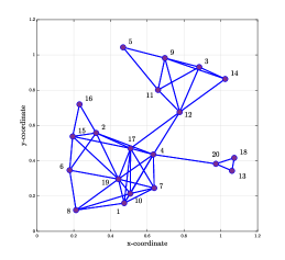
(a) Distributed network structure

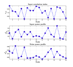
(b) Variances and correlation coefficients

Figure 3: A wireless network with $N=20$ nodes.

The simulated mean-square deviation (MSD) learning curves are obtained by ensemble averaging over 100 independent trials. We choose the same step sizes for all agents, i.e., $\mu_{k}=0.05$. The combining coefficients $a_{lk}$ are computed by the Metropolis rule. The evolution of the ensemble-average learning curves, $\frac{1}{N}\mathbb{E}[\|\widetilde{{\mathbf{w}}}_{i}\|^{2}]$, for the ATC diffusion strategy using different numbers of bits is assessed. The theoretical MSD of the DLMS with the same step size $\mu$ and the Metropolis rule applied to $a_{lk}$ is approximated by $\frac{\mu M}{N^{2}}\sum_{k=1}^{N}{\sigma_{v,k}^{2}}$ [5] and shown by curve 1. Curve 2 shows the standard DLMS performance assuming full resolution ADCs to perform system identification. Curves 3, 5 and 7 show the MSD evolution of the standard DLMS with low resolution signals coarsely quantized with 1, 2 and 3 bits, respectively. Curves 4, 6 and 8 show the MSD performance of the proposed DQA-LMS algorithm that improves the error measurement confronted with coarsely quantized signals. The performance of the proposed DQA-LMS algorithm is closer to the DLMS while it reduces about $90\%$ of the power consumption by ADCs in the network (see Fig. 2).

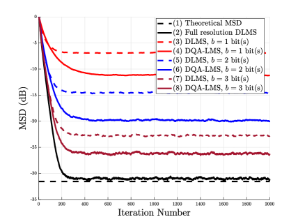
Figure 4: The MSD curves for the DLMS and DQA-LMS algorithms.

VI Conclusion

In this paper, we have proposed an energy-efficient framework for distributed learning and developed the DQA-LMS algorithm using low-resolution ADCs for adaptive IoT networks. DQA-LMS has comparable computational cost to the full-resolution DLMS algorithm while it enormously reduces the power consumption of the ADCs in the network. Simulations have shown the close performance of DQA-LMS to the DLMS algorithm despite dealing with coarsely quantized signals.

References

• [1] J. B. Predd, S. B. Kulkarni, and H. V. Poor, “Distributed learning in wireless sensor networks,” IEEE Signal Processing Magazine, vol. 23, no. 4, pp. 56–69, 2006.
• [2] M. M. Rana, W. Xiang, and E. Wang, “Iot-based state estimation for microgrids,” IEEE Internet of Things Journal, vol. 5, no. 2, pp. 1345–1346, 2018.
• [3] R. Olfati-Saber, J. A. Fax, and R. M. Murray, “Consensus and cooperation in networked multi-agent systems,” Proceedings of the IEEE, vol. 95, no. 1, pp. 215–233, 2007.
• [4] C. G. Lopes and A. H. Sayed, “Diffusion least-mean squares over adaptive networks: Formulation and performance analysis,” IEEE Transactions on Signal Processing, vol. 56, no. 7, pp. 3122–3136, 2008.
• [5] A. H. Sayed, S.-Y. Tu, J. Chen, X. Zhao, and Z. J. Towfic, “Diffusion strategies for adaptation and learning over networks: an examination of distributed strategies and network behavior,” IEEE Signal Processing Magazine, vol. 30, no. 3, pp. 155–171, 2013.
• [6] R. C. de Lamare and R. Sampaio-Neto, “Reduced-rank adaptive filtering based on joint iterative optimization of adaptive filters,” IEEE Signal Processing Letters, vol. 14, no. 12, pp. 980–983, 2007.
• [7] R. C. de Lamare and R. Sampaio-Neto, “Adaptive reduced-rank processing based on joint and iterative interpolation, decimation, and filtering,” IEEE Transactions on Signal Processing, vol. 57, no. 7, pp. 2503–2514, 2009.
• [8] S. Xu, R. C. de Lamare, and H. V. Poor, “Distributed estimation over sensor networks based on distributed conjugate gradient strategies,” IET Signal Processing, vol. 10, no. 3, pp. 291–301, 2016.
• [9] T. G. Miller, S. Xu, R. C. de Lamare, and H. V. Poor, “Distributed spectrum estimation based on alternating mixed discrete-continuous adaptation,” IEEE Signal Processing Letters, vol. 23, no. 4, pp. 551–555, 2016.
• [10] S. Xu, R. C. de Lamare, and H. V. Poor, “Distributed compressed estimation based on compressive sensing,” IEEE Signal Processing Letters, vol. 22, no. 9, pp. 1311–1315, Sep. 2015.
• [11] T. G. Miller, S. Xu, R. C. de Lamare, V. H. Nascimento, and Y. Zakharov, “Sparsity-aware distributed conjugate gradient algorithms for parameter estimation over sensor networks,” in 2015 49th Asilomar Conference on Signals, Systems and Computers. IEEE, 2015, pp. 1556–1560.
• [12] S. Xu, R. C. de Lamare, and H. V. Poor, “Distributed low-rank adaptive estimation algorithms based on alternating optimization,” Signal Processing, vol. 144, pp. 41 – 51, 2018.
• [13] S. Xu, R. C. de Lamare, and H. V. Poor, “Adaptive link selection algorithms for distributed estimation,” EURASIP Journal on Advances in Signal Processing, vol. 2015, no. 1, pp. 86, 2015.
• [14] S. Zhang and W. X. Zheng, “Distributed separated-decorrelation lms algorithms over sensor networks with noisy inputs,” IEEE Transactions on Signal Processing, vol. 68, pp. 4163–4177, 2020.
• [15] Y. Yu, H. Zhao, R. C. de Lamare, Y. Zakharov, and L. Lu, “Robust distributed diffusion recursive least squares algorithms with side information for adaptive networks,” IEEE Transactions on Signal Processing, vol. 67, no. 6, pp. 1566–1581, 2019.
• [16] C. Han, J. M. Jornet, E. Fadel, and I. F. Akyildiz, “A cross-layer communication module for the internet of things,” Computer Networks, vol. 57, no. 3, pp. 622–633, 2013.
• [17] I. Utlu, O. F. Kilic, and S. S. Kozat, “Resource-aware event triggered distributed estimation over adaptive networks,” Digital Signal Processing, vol. 68, pp. 127–137, 2017.
• [18] A. Mezghani and J. A. Nossek, “Power efficiency in communication systems from a circuit perspective,” in 2011 IEEE International Symposium of Circuits and Systems (ISCAS). IEEE, 2011, pp. 1896–1899.
• [19] R. H. Walden, “Analog-to-digital converter survey and analysis,” IEEE Journal on selected areas in communications, vol. 17, no. 4, pp. 539–550, 1999.
• [20] L. T. N. Landau and R. C. de Lamare, “Branch-and-bound precoding for multiuser MIMO systems with 1-bit quantization,” IEEE Wireless Communications Letters, vol. 6, no. 6, pp. 770–773, Dec 2017.
• [21] S. Jacobsson, G. Durisi, M. Coldrey, U. Gustavsson, and C. Studer, “Throughput analysis of massive MIMO uplink with low-resolution adcs,” IEEE Transactions on Wireless Communications, vol. 16, no. 6, pp. 4038–4051, 2017.
• [22] A. Mezghani, M.-S. Khoufi, and J. A. Nossek, “A modified MMSE receiver for quantized MIMO systems,” Proc. ITG/IEEE WSA, Vienna, Austria, pp. 1–5, 2007.
• [23] L. T. N. Landau, M. Dörpinghaus, R. C. de Lamare, and G. P. Fettweis, “Achievable rate with 1-bit quantization and oversampling using continuous phase modulation-based sequences,” IEEE Transactions on Wireless Communications, vol. 17, no. 10, pp. 7080–7095, Oct 2018.
• [24] Z. Shao, R. C. de Lamare, and L. T. N. Landau, “Iterative detection and decoding for large-scale multiple-antenna systems with 1-bit adcs,” IEEE Wireless Communications Letters, vol. 7, no. 3, pp. 476–479, June 2018.
• [25] Z. Shao, L. Landau, and R. C. de Lamare, “Adaptive RLS channel estimation and SIC for large-scale antenna systems with 1-bit ADCs,” in WSA 2018; 22nd International ITG Workshop on Smart Antennas. VDE, 2018, pp. 1–4.
• [26] Z. Shao, L. T. N. Landau, and R. C. de Lamare, “Channel estimation for large-scale multiple-antenna systems using 1-bit adcs and oversampling,” IEEE Access, vol. 8, pp. 85243–85256, 2020.
• [27] Z. Shao, L. T. N. Landau, and R. C. de Lamare, “Dynamic oversampling for 1-bit adcs in large-scale multiple-antenna systems,” IEEE Transactions on Communications, 2021.
• [28] A. Danaee, R. C. de Lamare, and V. H. Nascimento, “Energy-efficient distributed learning with coarsely quantized signals,” IEEE Signal Processing Letters, 2021.
• [29] J. J. Bussgang, “Crosscorrelation functions of amplitude-distorted gaussian signals. research lab. electron,” MIT, Cambridge, MA, USA, Tech. Rep, 1952.
• [30] S. Lloyd, “Least squares quantization in PCM,” IEEE transactions on information theory, vol. 28, no. 2, pp. 129–137, 1982.
• [31] J. Max, “Quantizing for minimum distortion,” IRE Transactions on Information Theory, vol. 6, no. 1, pp. 7–12, 1960.
• [32] Y. Li, C. Tao, G. Seco-Granados, A. Mezghani, A. L. Swindlehurst, and L. Liu, “Channel estimation and performance analysis of one-bit massive MIMO systems,” IEEE Transactions on Signal Processing, vol. 65, no. 15, pp. 4075–4089, 2017.
• [33] O. Orhan, E. Erkip, and S. Rangan, “Low power analog-to-digital conversion in millimeter wave systems: Impact of resolution and bandwidth on performance,” in 2015 Information Theory and Applications Workshop (ITA). IEEE, 2015, pp. 191–198.
• [34] R. Ratasuk, B. Vejlgaard, N. Mangalvedhe, and A. Ghosh, “Nb-iot system for M2M communication,” in 2016 IEEE wireless communications and networking conference. IEEE, 2016, pp. 1–5.
• [35] H. Chung, A. Rylyakov, Z. T. Deniz, J. Bulzacchelli, G Wei, and D. Friedman, “A 7.5-GS/s 3.8-ENOB 52-mW flash ADC with clock duty cycle control in 65nm CMOS,” in 2009 Symposium on VLSI Circuits. IEEE, 2009, pp. 268–269.
• [36] N. Takahashi, I. Yamada, and A. H. Sayed, “Diffusion least-mean squares with adaptive combiners: Formulation and performance analysis,” IEEE Transactions on Signal Processing, vol. 58, no. 9, pp. 4795–4810, 2010.