A reusable pipeline for large-scale fiber segmentation on unidirectional fiber beds using fully convolutional neural networks

Abstract

Fiber-reinforced ceramic-matrix composites are advanced materials resistant to high temperatures, with application to aerospace engineering. Their analysis depends on the detection of embedded fibers, with semi-supervised techniques usually employed to separate fibers within the fiber beds. Here we present an open computational pipeline to detect fibers in ex-situ X-ray computed tomography fiber beds. To separate the fibers in these samples, we tested four different architectures of fully convolutional neural networks. When comparing our neural network approach to a semi-supervised one, we obtained Dice and Matthews coefficients greater than $92.28\pm 9.65\%$, reaching up to $98.42\pm 0.03\%$, showing that the network results are close to the human-supervised ones in these fiber beds, in some cases separating fibers that human-curated algorithms could not find. The software we generated in this project is open source, released under a permissive license, and can be freely adapted and re-used in other domains. All data and instructions on how to download and use it are also available.

Keywords: Computer Vision, Deep Learning, Image Segmentation, 3D Analysis, Metrology.

1 INTRODUCTION

Fiber-reinforced ceramic-matrix composites are advanced materials used in aerospace gas-turbine engines [51, 35] and nuclear fusion [22], due to their resistance to temperatures 100–200 $\degree$C higher than allows for the same applications.

Larson et al. investigated new manufacturing processes for curing preceramic polymer into unidirectional fiber beds, studying the microstructure evolution during matrix impregnation and aiming to reinforce ceramic-matrix composites [24, 23]. They used X-ray computed tomography (CT) to characterize the three-dimensional microstructure of their composites non-destructively, studying their evolution in-situ while processing the materials at high temperatures [24] and describing overall fiber bed properties and microstructures of unidirectional composites [23]. The X-ray CT images acquired from these fiber beds are available at Materials Data Facility [5].

Larson et al.’s fiber beds have widths of approximately $1.5\,mm$, containing 5000–6200 fibers per stack. Each fiber has an average radius of $6.4\pm 0.9\,\mu m$, with diameters ranging from 13 to 20 pixels in the micrographs [23]. They present semi-supervised techniques to separate the fibers within the fiber beds; their segmentation is available for five samples [25]. However, we considered their results could be improved using different techniques. This motivated us to test alternative solutions.

In this study we separate fibers in ex-situ X-ray CT fiber beds of nine samples from Larson et al. The samples we used in this study correspond to two general states: wet — obtained after pressure removal — and cured. These samples were acquired using microtomographic instruments from the Advanced Light Source at Lawrence Berkeley National Laboratory operated in a low-flux, two-bunch mode [23]. We used their reconstructions obtained without phase retrieval; Larson et al. provide segmentations for five of these samples [25], which we compare to our results.

To separate the fibers in these samples, we tested four different fully convolutional neural networks (CNN, section 4.1), algorithms from computer vision and deep learning. When comparing our neural network approach to Larson et al. results, we obtained Dice [13] and Matthews [30] coefficients greater than $92.28\pm 9.65\%$, reaching up to $98.42\pm 0.03\%$, showing that the network results are close to the human-supervised ones in these fiber beds, in some cases separating fibers that the algorithms created by [23] could not find. All software and data generated in this study are available for download. Instructions are given for downloading the data and using the software. The code is open source, released under a permissive software license, and can be adapted easily for other domains.

2 RESULTS

Larson et al. provide segmentations for their fibers (Fig 1) in five of the wet and cured samples, obtained using the following pipeline [23]:

1. Fiber detection using the circular Hough transform [48, 3];

2. Correction of improperly identified pixels using filters based on connected region size and pixel value, and by comparisons using ten slices above and below the slice of interest;

3. Separation of fibers using the watershed algorithm [31].

.

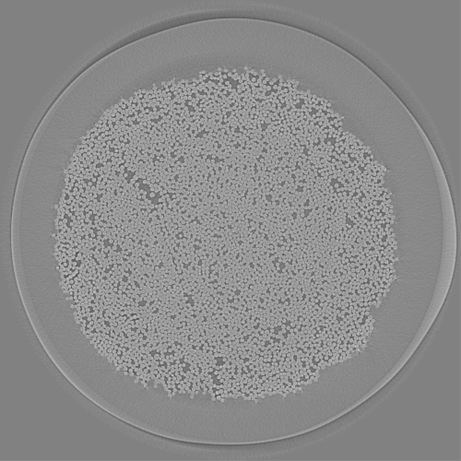
Figure 1: Slice number 1000 from the sample “232p3 wet”, provided in [25]. The whole sample contains 2160 slices. This slice represents the structure of the samples we processed: they contain the fiber bed (large circular structure) and the fibers within it (small round elements).

However, their proposed method briefly describes these steps. There are no details on parameters used, or the source code for their segmentation. We tried different approaches to reproduce their results, focusing on separating the fibers in the fiber bed samples. Our first approach was to create a classic, unsupervised image processing pipeline. We used histogram equalization [45], Chambolle’s total variation denoising [38, 7], multi-Otsu threshold [34, 28], and the WUSEM algorithm [12] to separate each single fiber. The result is a labeled image containing the separated fibers (Fig 2). The pipeline presented limitations when processing fibers on the edges of fiber beds, not being equivalent to the solution presented by Larson et al. We restricted the segmentation region to have a satisfactory result (Fig 2(d)), but the number of detected fibers is reduced.

.

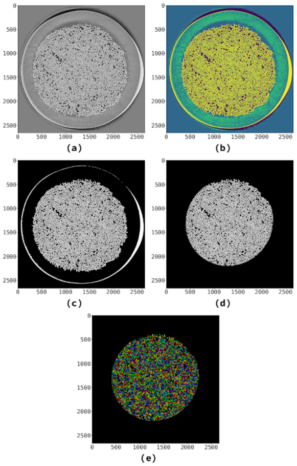
Figure 2: Rendering fibers detected in the limited region of interest by the classic pipeline. We exemplify the classic image processing pipeline using Fig 1 as the input image. This solution presented limitations when processing fibers on the edfes of fiber beds. (a) Histogram equalization and TV Chambolle’s filtering (parameter: weight=0.3). (b) Multi Otsu’s resulting regions (parameter: classes=4). Fibers are located within the fourth region (in yellow). (c) Binary image obtained considering region four in (b) as the region of interest, and the remaining regions as the background. (d) the processed region from (c), as shown in Fig 1. (e) Regions resulting from the application of WUSEM on the region shown in (d) (parameters: initial_radius=0, delta_radius=2, watershed_line=True). Colormaps: (a, c, d) gray, (b) viridis, (e) nipy_spectral.

To obtain more accurate results, we evaluated four fully convolutional neural network architectures: Tiramisu [19] and U-net [37], as well as their three-dimensional counterparts, 3D Tiramisu and 3D U-net [52]. We also investigated whether three-dimensional networks generate better segmentation results, leveraging the structure of the material.

2.1 Fully convolutional neural networks (CNN) for fiber detection

We implemented four architectures of fully convolutional neural networks (CNN) — Tiramisu, U-net, 3D Tiramisu, and 3D U-net — to reproduce the results provided by Larson et al. Labeled data, in our case, consists of fibers within fiber beds. To train the neural networks to recognize these fibers, we used slices from two different samples: 232p3 wet and 232p3 cured, registered according to the wet sample. Larson et al. provided the fiber segmentation for these samples [25], which we used as labels in the training. The training and validation datasets contained 250 and 50 images from each sample, respectively, in a total of 600 images. Each image from the original samples have width and height size of $2560\times 2560$ pixels.

During the training procedure, the networks reached accuracy higher than 0.9 and loss lower than 0.1 on the first epoch. Two-dimensional U-net is the exception, presenting loss of 0.23 at the end of the first epoch. Despite that, 2D U-net reaches the lowest loss between the four architectures at the end of its training. 2D U-net is also the fastest network to finish its training (7 h, 43 min), followed by Tiramisu (13 h, 10 min), 3D U-net (24 h, 16 min) and 3D Tiramisu (95 h, 49 min, Fig 3).

.

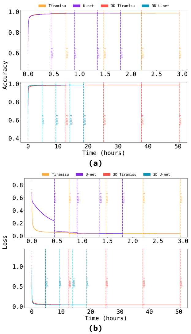
Figure 3: Accuracy (a) and loss (b) through time for each training epoch. All networks were trained during five epochs, reaching accuracy higher than 0.9 and loss lower than 0.1 on the first training epoch, except for the two-dimensional U-net. However, 2D U-net is the fastest to finish training, and reaches the lowest loss between the candidates. We attribute the subtle loss increase or accuracy decrease on the start of each epoch to the data augmentation process.

Still considering the 2D U-net, its convergence on the first epoch does not seem as stable as the other networks (Fig 4). However, this does not impair U-net’s accuracy (0.977 on the first epoch). Accuracy and loss for the validation dataset also improve significantly from the first epoch: Tiramisu had validation loss vs. validation accuracy ratio of 0.034 while U-net had 0.048, 3D Tiramisu had 0.043, and 3D U-net had 0.043 as well. We attribute these high accuracies and low losses to the large size of the training set and the similarities between slices in the input data.

.

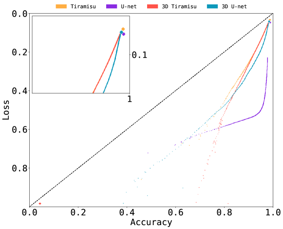
Figure 4: Accuracy vs. loss on the first epoch. Accuracy surpasses 0.9 and loss is lower than 0.1 for all networks during the first epoch, except for 2D U-net (loss of 0.23). The large size of the training set and the similarities in the data are responsible for such numbers. Validation accuracy and validation loss on the first epoch are represented by diamonds.

We used the coefficients from the training process to predict fibers in twelve different datasets in total. These datasets were made available by Larson et al [25], and we keep the same file identifiers for fast cross-reference:

• “232p1”: wet

• “232p3”: wet, cured, cured registered

• “235p1”: wet

• “235p4”: wet, cured, cured registered

• “244p1”: wet, cured, cured registered

• “245p1”: wet

Here, the first three numeric characters correspond to a material sample, and the last character correspond to different extrinsic factors, e.g. deformation. Despite being samples from similar materials, the reconstructed files presented several differences, for example regarding amount of ringing artifacts, intensity variation, noise, therefore they are considered as different samples in this paper.

We calculated the average processing time for each sample (Fig 5). The prediction time results are similar to the training ones; 2D U-net and 2D Tiramisu are the fastest architectures to process a sample, while 3D Tiramisu is the slowest.

.

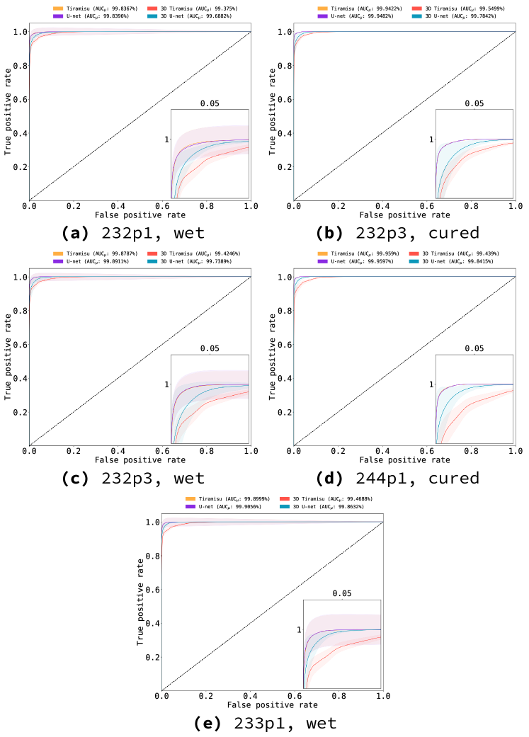
Figure 5: Mean and standard deviation for prediction times for each sample. As with processing, during training 2D U-net and 2D Tiramisu were the fastest architectures to process a sample in one hour, on average. 3D Tiramisu, being the slowest, takes in average more than a day to process one sample.

2.2 Evaluation of our results and comparison with Larson et al (2019)

After processing all samples, we compared our predictions with the results that Larson et al. made available on their dataset [25]. They provided five datasets from the twelve we processed: “232p1 wet”, “232p3 cured”, “232p3 wet”, “244p1 cured”, “244p1 wet”.

First, we compared our predictions to their results using receiver operating characteristic (ROC) curves and the area under curve (AUC, Fig 6). AUC is larger than 98% for all comparisons; therefore, our predictions are accurate when compared with the semi-supervised method suggested by Larson et al. The 2D versions of U-net and Tiramisu have similar results, performing better than 3D U-net and 3D Tiramisu.

.

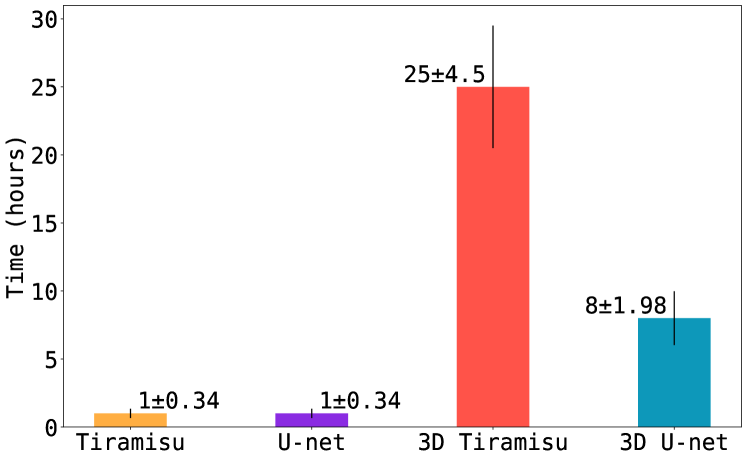
Figure 6: Receiver operating characteristic (ROC) and area under curve (AUC) from the comparison between the prediction for each network and the segmentation made available for five samples by Larson et al [25]. ROC curves were calculated to all slices in a dataset; their mean areas and standard deviation intervals are presented. AUC is larger than 98% in all comparisons, showing that our predictions are accurate when compared with Larson et al. semi-supervised method. The 2D versions of U-net and Tiramisu perform better when compared to their 3D alternatives.

We also examined the binary versions of our predictions and compared them with Larson et al. results. For each slice from the dataset, similarly to the volume, we used a hard threshold of $0.5$; values above that are considered as fibers, while values below that are treated as background. We used Dice [13] and Matthews [30] correlation coefficients for our comparison (1). The comparison using U-net yields the highest Dice and Matthews coefficients for three of five datasets. Tiramisu had highest Dice/Matthews coefficients for the “244p1, cured” dataset, and both networks have approximate results for “232p1, wet”. 3D Tiramisu had the lowest Dice and Matthews coefficients in our comparison.

	Tiramisu		U-net		3D Tiramisu		3D U-net
Sample	Dice	Matthews	Dice	Matthews	Dice	Matthews	Dice	Matthews
232p1, wet	$97.58\pm 2.29\%$	$96.55\pm 2.93\%$	$97.58\pm 2.20\%$	$96.60\pm 2.13\%$	$94.54\pm 6.73\%$	$92.28\pm 9.65\%$	$95.59\pm 0.74\%$	$93.71\pm 1.03\%$
232p3, cured	$98.21\pm 0.04\%$	$97.47\pm 0.06\%$	$98.26\pm 0.04\%$	$97.53\pm 0.06\%$	$95.25\pm 6.36\%$	$93.39\pm 8.88\%$	$95.90\pm 1.00\%$	$94.21\pm 1.30\%$
232p3, wet	$97.79\pm 2.15\%$	$96.87\pm 2.70\%$	$97.85\pm 2.12\%$	$96.98\pm 1.99\%$	$94.86\pm 6.90\%$	$92.76\pm 9.87\%$	$95.68\pm 1.97\%$	$93.92\pm 2.36\%$
244p1, cured	$98.42\pm 0.03\%$	$97.83\pm 0.05\%$	$98.38\pm 0.04\%$	$97.78\pm 0.05\%$	$94.55\pm 7.74\%$	$92.67\pm 10.54\%$	$96.30\pm 1.25\%$	$94.97\pm 1.54\%$
244p1, wet	$98.08\pm 2.53\%$	$97.39\pm 3.15\%$	$98.10\pm 2.39\%$	$97.43\pm 2.23\%$	$94.81\pm 7.81\%$	$92.97\pm 10.71\%$	$96.67\pm 1.00\%$	$95.45\pm 1.31\%$

Table 1: Dice and Matthews coefficients for each sample, obtained from the comparison of our neural network results and data from Larson et al [25]. U-net yields the highest Dice and Matthews coefficients for three of five samples. Tiramisu had highest Dice/Matthews coefficients for one of the datasets. 3D Tiramisu had the lowest Dice and Matthews coefficients.

3 DISCUSSION

The analysis of ceramic matrix composites (CMC) depends on the detection of its fibers. Semi-supervised algorithms such as the one presented by Larson et al [23] can perform satisfactorily for that end. However, their specific algorithm lack information on the parameters necessary for replication. Reimplementing such methods without that information would lead to inaccurate results, since the reported approach includes manual steps that require human curation.

Convolutional neural networks are being used successfully in the segmentation of different two- and three-dimensional scientific data (e.g., [4, 43, 16, 29, 39, 27]), including microtomographies. For example, fully convolutional neural networks were used to generate 3D tau inclusion density maps [2], to segment the tidemark on osteochondral samples [42], and 3D models of structures of temporal-bone anatomy [33].

Researchers are studying fiber-analysis detection for a while, using different tools. There are several approaches using tracking, statistical approaches, or classical image processing (e.g., [10, 6, 40, 44, 50, 14, 15, 9]). To the best of our knowledge, there are two different deep learning approaches for this problem:

• Yu et al. [47] use an unsupervised learning approach based on Faster R-CNN [36] and a Kalman filter based tracking. They compare their results with Zhou et al. [50], reaching a Dice coefficient of up to 99 %.

• Miramontes et al. [32] reach an average accuracy of 93.75% using a 2D LeNet-5 CNN [26] to detect fibers in a specific sample.

Our study builds upon previous work by using similar material samples, but it expands tests to many more samples as well as it includes the implemention and training of four architectures: 2D U-net, 2D Tiramisu, 3D U-net, and 3D Tiramisu, used to process twelve large datasets ($\approx$ 140 GB), and comparing our results with the gold standard data provided by Larson et al. [25] for five of them. We used ROC curves and their area under curve (AUC) to ensure the quality of our predictions, obtaining AUC larger than 98% (Fig 6). Also, Dice and Matthews coefficients were used to compare our results with Larson et al’s solutions (Table 1), reaching coefficients of up to $98.42\pm 0.03\%$.

When processing a defective slice, the 3D architectures perform better when compared to the 2D ones, since they leverage from information of the material structure (Fig 7).

.

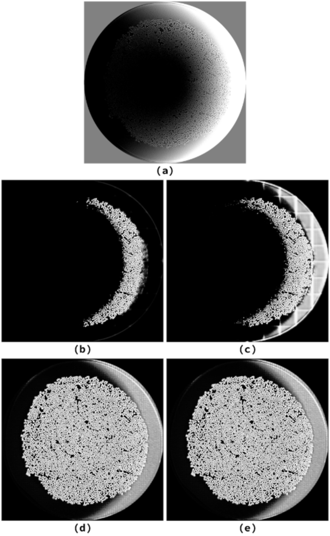
Figure 7: A defective slice on the sample “232p3 wet” and the segmentation resulting from each architecture. While the 2D architectures results are impaired by the defects present in the input image, the 3D ones leverage from the sample structure to present a better segmentation result. (a) Original defective image, (b) U-net prediction, (c) 3D U-net prediction, (d) Tiramisu prediction, (e) 3D Tiramisu prediction.

Based on our research, we recommend using the 2D U-net to process microtomographies of CMC fibers. Both 2D networks lead to similar accuracy and loss values (1) in our comparisons; however, U-nets achieve these numbers in a shorter time, when compared to Tiramisu. The 3D architectures, while presenting the advantage of performing better in defective samples (Fig 7), do not achieve general results comparable to the 2D architectures. Satisfactory results using the 3D architectures could be achieved with more training time; however, one should notice that the training we proposed (Fig 3) and the consequent predictions (Fig 5) required a considerable computing time, and more training could lead to marginal improvements when compared to their 2D alternatives.

Our CNN architectures perform to the level of human-curated accuracy — i.e., Larson et al. semi-supervised approach —, sometimes even surpassing Larson et al. algorithm. For instance, the 2D U-net process fibers their algorithm could not find (Fig 8).

.

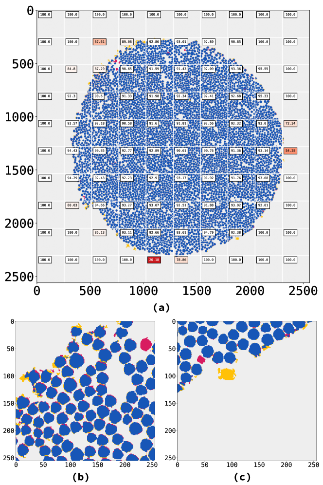
Figure 8: Visual comparison between 2D U-net and Larson et al. results for sample “232p3 wet”. Each part of this image is obtained combining both ours and Larson et al.’s results; we compared each slice, and presented the ones that return the lowest Matthews comparison coefficient. Labels present the Matthews coefficient for each slice. (b, c) slices presenting fibers found only by U-net (in red), while some well-defined structures close to the borders are found only by Larson et al. (in yellow). Slice size: $256\times 256$. Colors set according to the comparison. Blue: true positives; red: false positives; yellow: false negatives; gray: true negatives. For more details on the comparison coefficients, please see 4.2.

Using the data processed by the U-net architecture, we can render a three-dimensional visualization of the fibers (Fig 9). Despite the absence of tracking, the segmentation provided by the U-net identifies the fibers across the stack.

.

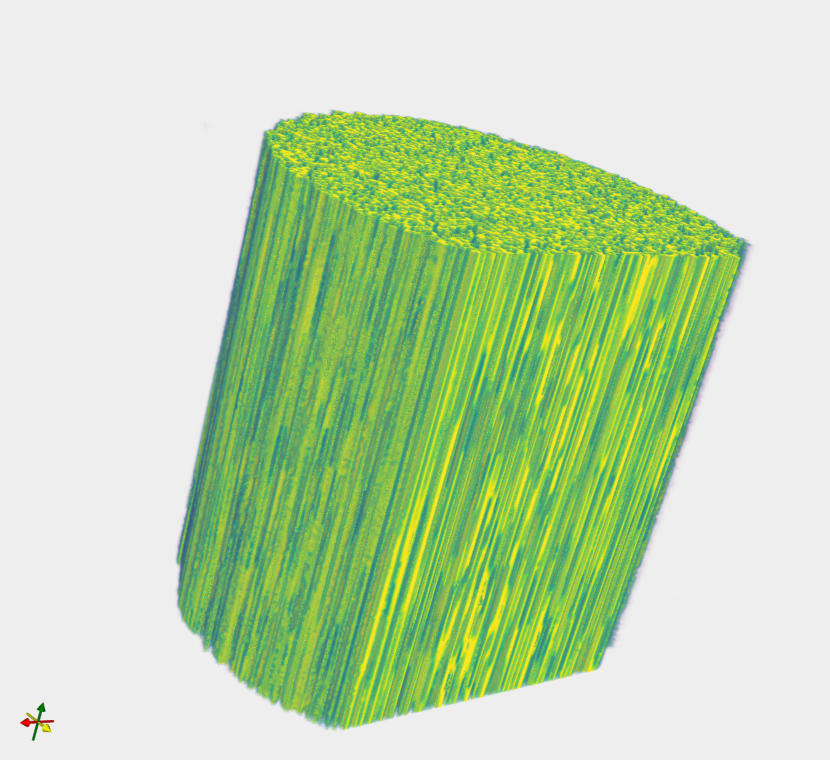
Figure 9: Fibers on the sample “232p3 wet” processed using the U-net architecture. As seen in the longitudinal cut, this pipeline identifies fibers across the sample height despite the absence of tracking.

In this paper, we presented deep learning solutions to analyze microtomographies of CMC fibers in fiber beds. The data used is publicly available [25] and was acquired in a real materials design experiment. Our solutions are comparable to human-curated results, being capable of predicting fibers in large stacks of microtomographies without human intervention.

Despite the encouraging results we achieved in this study, there is further space for improvements. For example, we aim to study how an ensemble of our trained networks would perform in these samples. Another proposal would be to work with different thresholds at the last layer of your network. We maintained a hard threshold of $0.5$, that suited the sigmoid on the last layer of the CNN we implemented. We could also use conditional random field networks for that end.

4 METHODS

4.1 Fully convolutional neural networks

We implemented four architectures — two dimensional U-net [37] and Tiramisu [19], and their three-dimensional versions — to attempt reproducing the results provided by Larson et al. We used supervised algorithms: they rely on labeled data to learn what are the regions of interest — in our case, fibers within microtomographies of fiber beds.

All CNN algorithms were implemented using TensorFlow [1] and Keras [8] on a computer with two Intel Xeon Gold processors 6134 and two Nvidia GeForce RTX 2080 graphical processing units. Each GPU has 10 GB of RAM.

To train the neural networks on how to recognize the fibers, we used slices from two different samples: “232p3 wet” and “232p3 cured”, registered according to the wet sample. Larson et al. provided the fiber segmentation for these samples, which we used as labels in the training. The training and validation procedures processed 350 and 149 images from each sample, respectively; a total of 998 images. Each image from the original samples have width and height size of $2560\times 2560$ pixels.

To feed the two-dimensional networks, we padded the images with 16 pixels, of value zero, in each dimension. Then, each image was cut into tiles of size $288\times 288$, each 256 pixels, creating an overlap of 32 pixels. These overlapping regions, which are again removed after processing, avoid artifacts on the borders of processed tiles. Therefore, each input slice generated 100 images with $288\times 288$ pixels, in a total of 50,000 images for the training set, and 10,000 for the validation set.

We needed to pre-process the training images differently to train the three-dimensional networks. We loaded the entire samples, each with size $2160\times 2560\times 2560$, and padded their dimensions with 16 pixels. Then, we cut slices of size $64\times 64\times 64$ voxels, each 32 pixels. Hence, the training and validation sets for the three-dimensional networks have 96,000 and 19,200 cubes, respectively.

We implemented data augmentation in our pipeline, aiming for a network capable of processing samples with different characteristics. We augmented the images on the training sets using rotations, horizontal and vertical flips, width and height shifts, zoom and shear transforms. For that, we used Keras embedded tools within the ImageDataGenerator module to augment images for the two-dimensional networks. Since Keras’s ImageDataGenerator is not able to process three-dimensional input so far, we adapted the ImageDataGenerator module. The adapted version we used in this study is named ChunkDataGenerator, and is available in the Supplementary Material.

To reduce the possibility of overfitting, we implemented dropout regularization [41] in our pipeline. We followed the suggestions in the original papers for U-net architectures: 2D U-net received a dropout rate of 50% in the last analysis layer and in the bottleneck, while 3D U-net [52] did not receive any dropout. The Tiramisu structures received a dropout rate of 20%, as suggested by Jégou et al [19].

For a better comparison, we maintained the same training hyperparameters when possible. Due to the large amount of training data and the similarities between training samples (2D tiles or 3D cubes), our preliminary tests indicated that we would have a higher accuracy for all networks in the first training epochs. Therefore, we decided to train all architectures during five epochs. The 2D architectures were trained with batches of four images, while the batches for 3D architectures had two cubes each. For all architectures, we used a learning rate of $1E-4$, and binary cross entropy [49] as the loss function. We followed the original papers regarding to optimization algorithms: we used the Adam optimizer [20] in the U-net architectures, while the Tiramisu ones were trained using the RMSProp optimizer [11]. We implemented batch normalization [18] in all architectures, including the 2D U-net. Ronneberger et al. do not suggest it in their preliminary study, although it is known that architectures using batch normalization tend to converge faster.

4.2 Evaluation

We used Dice [13] and Matthews [30] correlation coefficients (Equations 1, 2]) to evaluate our results, assuming that the fiber detections from [25] contain a reasonable gold standard.

$$Dice=\frac{2\times TP}{2\times TP+FP+FN}$$ (1)

$$Matthews=\frac{TP\times TN-FP\times FN}{\sqrt{(TP+FN)(TP+FP)(TN+FN)(TN+FP)}}$$ (2)

Dice and Matthews coefficients receive true positive (TP), false positive (FP), true negative (TN), and false negative (FN) pixels, which are determined as:

• TP: pixels correctly labeled as being part of a fiber.

• FP: pixels incorrectly labeled as being part of a fiber.

• TN: pixels correctly labeled as background.

• FN: pixels incorrectly labeled as background.

TP, FP, TN, and FN are obtained when the prediction data is compared with a certain gold standard, which in this study is Larson’s semi-supervised segmentation data [25].

4.3 Visualization

Imaging CMC specimens at high-resolution as Larson et al samples [25] leads to large datasets — each stack we used in this paper has around 14 GB after the reconstruction, for example.

Frequently, the specialist needs software to visualize the result of their data collection, but most of them fail to produce meaningful graphs without considering advanced image analysis and/or computational platforms with generous amounts of memory. One may use Jupyter Notebooks [21], which enable domain scientists to quickly probe specimens imaged with X-ray microCT during their beamtime. For this reason, the figures in this paper are all generated on standard laptops with no more than 16 GB of RAM, which is the typical computation system at hand.

We used matplotlib [17] and ITK [46] (Fig 9) to generate our figures. Despite our use of methods that consider either global or local information, we designed protocols that allow any user to visualize essential content from their experiments recorded as 3D image stacks.

5 DATA AVAILABILITY

The supplementary data generated in this study is available at https://datadryad.org/stash/dataset/doi:10.6078/D1069R, under a CC0 (public domain) license.

6 CODE AVAILABILITY

The software we produced throughout this study is available at https://github.com/alexdesiqueira/fcn_microct/, under a BSD license.

7 ACKNOWLEDGEMENTS

AFS would like to thank Sebastian Berg, Ross Barnowski, Silvia Miramontes, Ralf Gommers, and Matt Rocklin for the discussions on fully convolutional networks, their structure and different frameworks. This research was funded in part by the Gordon and Betty Moore Foundation through Grant GBMF3834 and by the Alfred P. Sloan Foundation through Grant 2013-10-27 to the University of California, Berkeley.

References

- [1] Martín Abadi, Paul Barham, Jianmin Chen, Zhifeng Chen, Andy Davis, Jeffrey Dean, Matthieu Devin, Sanjay Ghemawat, Geoffrey Irving, Michael Isard, and et al. Tensorflow: a system for large-scale machine learning. In Proceedings of the 12th USENIX conference on Operating Systems Design and Implementation, OSDI’16, page 265–283. USENIX Association, Nov 2016.
- [2] Maryana Alegro, Yuheng Chen, Dulce Ovando, Helmut Heinser, Rana Eser, Daniela Ushizima, Duygu Tosun, and Lea T. Grinberg. Deep learning for alzheimer’s disease: Mapping large-scale histological tau protein for neuroimaging biomarker validation. bioRxiv, page 698902, May 2020.
- [3] T. J. Atherton and D. J. Kerbyson. Size Invariant Circle Detection. 1999.
- [4] Samik Banerjee, Lucas Magee, Dingkang Wang, Xu Li, Bing-Xing Huo, Jaikishan Jayakumar, Katherine Matho, Meng-Kuan Lin, Keerthi Ram, Mohanasankar Sivaprakasam, and et al. Semantic segmentation of microscopic neuroanatomical data by combining topological priors with encoder–decoder deep networks. Nature Machine Intelligence, 2(1010):585–594, Oct 2020.
- [5] B. Blaiszik, K. Chard, J. Pruyne, R. Ananthakrishnan, S. Tuecke, and I. Foster. The materials data facility: Data services to advance materials science research. JOM, 68(8):2045–2052, August 2016.
- [6] Stephen Bricker, J. P. Simmons, Craig Przybyla, and Russell Hardie. Anomaly detection of microstructural defects in continuous fiber reinforced composites. page 94010A, Mar 2015.
- [7] A. Chambolle. An algorithm for total variation minimization and applications. Journal of Mathematical Imaging and Vision, 20(1):89–97, 2004.
- [8] François Chollet et al. Keras. https://keras.io, 2015.
- [9] Peter J. Creveling, William W. Whitacre, and Michael W. Czabaj. A fiber-segmentation algorithm for composites imaged using x-ray microtomography: Development and validation. Composites Part A: Applied Science and Manufacturing, 126:105606, Nov 2019.
- [10] Michael W. Czabaj, Mark L. Riccio, and William W. Whitacre. Numerical reconstruction of graphite/epoxy composite microstructure based on sub-micron resolution x-ray computed tomography. Composites Science and Technology, 105:174–182, Dec 2014.
- [11] Yann N. Dauphin, Harm de Vries, and Yoshua Bengio. Equilibrated adaptive learning rates for non-convex optimization. arXiv:1502.04390 [cs], Feb 2015. arXiv: 1502.04390.
- [12] Alexandre Fioravante de Siqueira, Wagner Massayuki Nakasuga, Sandro Guedes, and Lothar Ratschbacher. Segmentation of nearly isotropic overlapped tracks in photomicrographs using successive erosions as watershed markers. Microscopy Research and Technique, 0(0):0, 2019.
- [13] Lee R. Dice. Measures of the amount of ecologic association between species. Ecology, 26(3):297–302, Jul 1945.
- [14] Monica J. Emerson, Kristine M. Jespersen, Anders B. Dahl, Knut Conradsen, and Lars P. Mikkelsen. Individual fibre segmentation from 3d x-ray computed tomography for characterising the fibre orientation in unidirectional composite materials. Composites Part A: Applied Science and Manufacturing, 97:83–92, Jun 2017.
- [15] Monica Jane Emerson, Vedrana Andersen Dahl, Knut Conradsen, Lars Pilgaard Mikkelsen, and Anders Bjorholm Dahl. Statistical validation of individual fibre segmentation from tomograms and microscopy. Composites Science and Technology, 160:208–215, May 2018.
- [16] James P. Horwath, Dmitri N. Zakharov, Rémi Mégret, and Eric A. Stach. Understanding important features of deep learning models for segmentation of high-resolution transmission electron microscopy images. npj Computational Materials, 6(11):1–9, Jul 2020.
- [17] J. D. Hunter. Matplotlib: A 2d graphics environment. Computing in Science & Engineering, 9(3):90–95, 2007.
- [18] Sergey Ioffe and Christian Szegedy. Batch normalization: Accelerating deep network training by reducing internal covariate shift. arXiv:1502.03167 [cs], Mar 2015. arXiv: 1502.03167.
- [19] Simon Jégou, Michal Drozdzal, David Vazquez, Adriana Romero, and Yoshua Bengio. The one hundred layers tiramisu: Fully convolutional densenets for semantic segmentation. arXiv:1611.09326 [cs], Oct 2017. arXiv: 1611.09326.
- [20] Diederik P. Kingma and Jimmy Ba. Adam: A method for stochastic optimization. arXiv:1412.6980 [cs], Jan 2017. arXiv: 1412.6980.
- [21] Thomas Kluyver, Benjamin Ragan-Kelley, Fernando Pérez, Brian Granger, Matthias Bussonnier, Jonathan Frederic, Kyle Kelley, Jessica Hamrick, Jason Grout, Sylvain Corlay, Paul Ivanov, Damián Avila, Safia Abdalla, and Carol Willing. Jupyter notebooks – a publishing format for reproducible computational workflows. In F. Loizides and B. Schmidt, editors, Positioning and Power in Academic Publishing: Players, Agents and Agendas, pages 87 – 90. IOS Press, 2016.
- [22] T. Koyanagi, Y. Katoh, T. Nozawa, L. L. Snead, S. Kondo, C. H. Henager, M. Ferraris, T. Hinoki, and Q. Huang. Recent progress in the development of sic composites for nuclear fusion applications. Journal of Nuclear Materials, 511:544–555, Dec 2018.
- [23] Natalie M. Larson, Charlene Cuellar, and Frank W. Zok. X-ray computed tomography of microstructure evolution during matrix impregnation and curing in unidirectional fiber beds. Composites Part A: Applied Science and Manufacturing, 117:243–259, February 2019.
- [24] Natalie M. Larson and Frank W. Zok. In-situ 3d visualization of composite microstructure during polymer-to-ceramic conversion. Acta Materialia, 144:579–589, Feb 2018.
- [25] Natalie M. Larson and Frank W. Zok. Ex-situ xct dataset for ”x-ray computed tomography of microstructure evolution during matrix impregnation and curing in unidirectional fiber beds”. http://dx.doi.org/doi:10.18126/M2QM0Z, 2019.
- [26] Y. Lecun, L. Bottou, Y. Bengio, and P. Haffner. Gradient-based learning applied to document recognition. Proceedings of the IEEE, 86(11):2278–2324, Nov 1998.
- [27] Wei Li, Kevin G. Field, and Dane Morgan. Automated defect analysis in electron microscopic images. npj Computational Materials, 4(11):1–9, Jul 2018.
- [28] P.-S. Liao, T.-S. Chen, and P.-C. Chung. A fast algorithm for multilevel thresholding. Journal of Information Science and Engineering, 17(5):713–727, 2001.
- [29] Boyuan Ma, Xiaoyan Wei, Chuni Liu, Xiaojuan Ban, Haiyou Huang, Hao Wang, Weihua Xue, Stephen Wu, Mingfei Gao, Qing Shen, and et al. Data augmentation in microscopic images for material data mining. npj Computational Materials, 6(11):1–9, Aug 2020.
- [30] Brian W. Matthews. Comparison of the predicted and observed secondary structure of t4 phage lysozyme. Biochimica et Biophysica Acta (BBA) - Protein Structure, 405(2):442–451, 1975.
- [31] Fernand Meyer. Topographic distance and watershed lines. Signal Processing, 38(1):113–125, July 1994.
- [32] Silvia Miramontes, Daniela M. Ushizima, and Dilworth Y. Parkinson. Evaluating fiber detection models using neural networks. In George Bebis, Richard Boyle, Bahram Parvin, Darko Koracin, Daniela Ushizima, Sek Chai, Shinjiro Sueda, Xin Lin, Aidong Lu, Daniel Thalmann, and et al., editors, Advances in Visual Computing, Lecture Notes in Computer Science, page 541–552. Springer International Publishing, 2019.
- [33] Soodeh Nikan, Sumit K. Agrawal, and Hanif M. Ladak. Fully automated segmentation of the temporal bone from micro-ct using deep learning. In Medical Imaging 2020: Biomedical Applications in Molecular, Structural, and Functional Imaging, volume 11317, page 113171U. International Society for Optics and Photonics, Feb 2020.
- [34] N. Otsu. A threshold selection method from gray-level histograms. IEEE Transactions on Systems, Man and Cybernetics, 9(1):62–66, 1979.
- [35] Nitin P. Padture. Advanced structural ceramics in aerospace propulsion. Nature Materials, 15(8):804–809, Aug 2016.
- [36] Shaoqing Ren, Kaiming He, Ross Girshick, and Jian Sun. Faster r-cnn: Towards real-time object detection with region proposal networks. IEEE transactions on pattern analysis and machine intelligence, 39(6):1137–1149, 2017.
- [37] Olaf Ronneberger, Philipp Fischer, and Thomas Brox. U-Net: Convolutional Networks for Biomedical Image Segmentation. In Nassir Navab, Joachim Hornegger, William M. Wells, and Alejandro F. Frangi, editors, Medical Image Computing and Computer-Assisted Intervention – MICCAI 2015, Lecture Notes in Computer Science, pages 234–241. Springer International Publishing, 2015.
- [38] Leonid I. Rudin, Stanley Osher, and Emad Fatemi. Nonlinear total variation based noise removal algorithms. Physica D: Nonlinear Phenomena, 60(1):259–268, 1992.
- [39] Yu Saito, Kento Shin, Kei Terayama, Shaan Desai, Masaru Onga, Yuji Nakagawa, Yuki M. Itahashi, Yoshihiro Iwasa, Makoto Yamada, and Koji Tsuda. Deep-learning-based quality filtering of mechanically exfoliated 2d crystals. npj Computational Materials, 5(11):1–6, Dec 2019.
- [40] R. M. Sencu, Z. Yang, Y. C. Wang, P. J. Withers, C. Rau, A. Parson, and C. Soutis. Generation of micro-scale finite element models from synchrotron x-ray ct images for multidirectional carbon fibre reinforced composites. Composites Part A: Applied Science and Manufacturing, 91:85–95, Dec 2016.
- [41] Nitish Srivastava, Geoffrey Hinton, Alex Krizhevsky, Ilya Sutskever, and Ruslan Salakhutdinov. Dropout: a simple way to prevent neural networks from overfitting. The Journal of Machine Learning Research, 15(1):1929–1958, Jan 2014.
- [42] Aleksei Tiulpin, Mikko Finnilä, Petri Lehenkari, Heikki J. Nieminen, and Simo Saarakkala. Deep-learning for tidemark segmentation in human osteochondral tissues imaged with micro-computed tomography. In Jacques Blanc-Talon, Patrice Delmas, Wilfried Philips, Dan Popescu, and Paul Scheunders, editors, Advanced Concepts for Intelligent Vision Systems, Lecture Notes in Computer Science, page 131–138. Springer International Publishing, 2020.
- [43] Yuta Tokuoka, Takahiro G. Yamada, Daisuke Mashiko, Zenki Ikeda, Noriko F. Hiroi, Tetsuya J. Kobayashi, Kazuo Yamagata, and Akira Funahashi. 3d convolutional neural networks-based segmentation to acquire quantitative criteria of the nucleus during mouse embryogenesis. npj Systems Biology and Applications, 6(11):1–12, Oct 2020.
- [44] Daniela M. Ushizima, Hrishikesh A. Bale, E. Wes Bethel, Peter Ercius, Brett A. Helms, Harinarayan Krishnan, Lea T. Grinberg, Maciej Haranczyk, Alastair A. Macdowell, Katarzyna Odziomek, and et al. Ideal: Images across domains, experiments, algorithms and learning. JOM, 68(11):2963–2972, Nov 2016.
- [45] R.E. Woods and R.C. Gonzalez. Real-time digital image enhancement. Proceedings of the IEEE, 69(5):643–654, May 1981.
- [46] Terry S Yoo, Michael J Ackerman, William E Lorensen, Will Schroeder, Vikram Chalana, Stephen Aylward, Dimitris Metaxas, and Ross Whitaker. Engineering and algorithm design for an image processing api: A technical report on itk - the insight toolkit. Studies in health technology and informatics, pages 586–592, 2002.
- [47] Hongkai Yu, Dazhou Guo, Zhipeng Yan, Wei Liu, Jeff Simmons, Craig P. Przybyla, and Song Wang. Unsupervised learning for large-scale fiber detection and tracking in microscopic material images. arXiv:1805.10256 [cs], May 2018. arXiv: 1805.10256.
- [48] H. K. Yuen, J. Princen, J. Dlingworth, and J. Kittler. A Comparative Study of Hough Transform Methods for Circle Finding. In Procedings of the Alvey Vision Conference 1989, pages 29.1–29.6, Reading, 1989. Alvey Vision Club.
- [49] Zhilu Zhang and Mert R. Sabuncu. Generalized cross entropy loss for training deep neural networks with noisy labels. In Proceedings of the 32nd International Conference on Neural Information Processing Systems, NIPS’18, page 8792–8802. Curran Associates Inc., Dec 2018.
- [50] Youjie Zhou, Hongkai Yu, Jeff Simmons, Craig P. Przybyla, and Song Wang. Large-scale fiber tracking through sparsely sampled image sequences of composite materials. IEEE Transactions on Image Processing, 25(10):4931–4942, Oct 2016.
- [51] Frank W Zok. Ceramic-matrix composites enable revolutionary gains in turbine engine efficiency. American Ceramic Society Bulletin, 95(5):7, 2016.
- [52] Özgün Çiçek, Ahmed Abdulkadir, Soeren S. Lienkamp, Thomas Brox, and Olaf Ronneberger. 3d u-net: Learning dense volumetric segmentation from sparse annotation. arXiv:1606.06650 [cs], Jun 2016. arXiv: 1606.06650.