Comment on “The Winfree model with non-infinitesimal phase-response curve: Ott-Antonsen theory” [Chaos 30, 073139 (2020)]

Abstract

This article may be downloaded for personal use only. Any other use requires prior permission of the author and AIP Publishing. This article appeared in Chaos 31, 018101 (2021) and may be found here

In a recent paper [Chaos 30, 073139 (2020)] we analyzed an extension of the Winfree model with nonlinear interactions. The nonlinear coupling function $Q$ was mistakenly identified with the non-infinitesimal phase-response curve (PRC). Here, we asses to what extent $Q$ and the actual PRC differ in practice. By means of numerical simulations, we compute the PRCs corresponding to the $Q$ functions previously considered. The results confirm a qualitative similarity between the PRC and the coupling function $Q$ in all cases.

In Ref. Pazó and Gallego (2020) we studied this generalization of the Winfree model of globally coupled phase oscillators:

$$\dot{\theta}_{i} = \omega_{i}+Q(\theta_{i},A),$$ (1a)

$$A = \frac{\epsilon}{N}\sum_{j=1}^{N}P(\theta_{j}).$$ (1b)

Here, $A$ is proportional to the sum over the pulses emitted by the $N$ oscillators of the population. In contrast to the original model Winfree (1967, 1980), function $Q$ in Eq. (1a) has a nonlinear dependence on the mean field $A$. The motivation for this is the fact that nonlinearity is an unavoidable consequence of applying phase reduction beyond the first order to oscillator ensembles Rosenblum and Pikovsky (2019). Note that a Taylor expansion of $Q$ to $n$th order in $A$ yields up to $(n+1)$-body phase interactions, similarly to Ref. León and Pazó (2019).

We mistakenly called $Q$ ‘non-infinitesimal phase-response curve’ in Ref. Pazó and Gallego (2020). Properly speaking, function $Q$ is a non-linear ‘coupling function’ Rosenblum and Pikovsky (2019). The aim of this comment is to clarify to what extent the coupling function $Q$ determines the actual phase-response curve (PRC). The PRC quantifies the phase shift gained by an oscillator in response to an external stimulus Izhikevich (2007). There is no analytic relation between $Q$ and the PRC beyond the small $\epsilon$ limit; in that case $Q(\theta,A)\simeq\tilde{Q}(\theta)A$, where $\tilde{Q}$ turns out to be so-called infinitesimal PRC (iPRC). In consequence, we rely here on numerical simulations to compute the PRC empirically.

The family of functions $Q(\theta,A)$ considered in Pazó and Gallego (2020) was:

$$Q(\theta,A)=f_{1}(A)(1-\cos\theta)-f_{2}(A)\sin\theta.$$ (2)

Four representative pairs of functions $f_{1,2}(A)$ were studied in detail in Pazó and Gallego (2020) and the corresponding coupling functions $Q(\theta,A)$ were depicted in Fig. 2 of Ref. Pazó and Gallego (2020). With the aim of comparing them, we obtain the PRC for each of the four coupling functions $Q$ considered in Pazó and Gallego (2020).

The PRC value depends on the timing as well as on the specific shape of the stimulus, which is not necessarily weak or brief  Izhikevich (2007). Numerically, we obtain the PRC measuring the effect on one oscillator’s phase of a pulse generated by another oscillator. This means that the two oscillators are unidirectionally coupled (i.e., a master-slave configuration). We adopt $\omega=1$ as the natural frequency for both, perturbed and perturbing oscillators, which is the obvious choice as it is the central frequency of the distribution in Pazó and Gallego (2020). Moreover, we follow Pazó and Gallego (2020) and use the same $2\pi$-periodic symmetric unimodal pulse function $P(\theta)$. It vanishes at $\theta=\pm\pi$, and a free parameter $r<1$ controls the narrowness of $P$: The height of the pulse is $P(0)=2/(1-r)$, and $\lim_{r\to 1}P(\theta)=2\pi\delta(\theta)$. In this comment we consider two different pulse widths: $r=0.9$ (the value selected in Pazó and Gallego (2020)), and $r=0.99$ corresponding to an extremely narrow pulse.

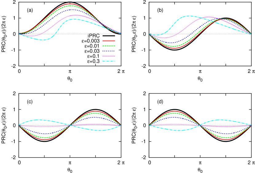
Figure 1: PRCs for cases (a-d) in Ref. Pazó and Gallego (2020). The set of five $\epsilon$ values used in indicated in panel (a). The coupling function (2) in each panel is: (a) $f_{1}=A/(1+A)=f_{2}/A$; (b) $f_{1}=A^{2}/(1+A)=Af_{2}$; (c) $f_{1}=0$, $f_{2}=A(1-A)/(1+A)$; (d) $f_{1}=0$, $f_{2}=A(A-1)/(1+A)$. The pulse acting on the oscillator is $P(t-\pi)=\frac{(1-r)[1+\cos(t-\pi)]}{1-2r\cos(t-\pi)+r^{2}}$, with $r=0.9$.

The simulation starts at time $t=0$ with the (slave) oscillator at an initial phase $\theta_{\rm in}$. Then, we let it to evolve under the influence of the forcing oscillator. The phase of this one grows linearly, such that the input felt by the first oscillator is $A(t)=\epsilon P(t-\pi)$. Parameter $\epsilon$ determines the strength of the stimulus. The simulation runs from $t=0$ to $t=2\pi$, since $A$ exactly vanishes at these times. Note that we do not need to run the simulation further since phase oscillators are governed by first-order differential equations. For a given $\epsilon$ value, we measure the phase shift at $t=2\pi$ such that $\mathrm{PRC}(\theta_{0},\epsilon)=\theta(t=2\pi)-(\theta_{\rm in}+2\pi)$. The phase $\theta_{0}$ in the argument of the PRC is the phase value when $A$ attains its maximum, assuming no input exists: $\theta_{0}=\theta_{\rm in}+\pi$. The results are shown in Figs. 1 and 2 for a set of $\epsilon$ values; in each panel for one particular coupling function $Q(\theta,A)$ already adopted in Pazó and Gallego (2020). In all panels, the corresponding iPRC is shown as a reference. Note that the normalization of the $y$-axis in Figs. 1 and 2 includes a $2\pi$ factor —in addition to $\epsilon$— because this is the integral of the pulse over an interval of length $2\pi$. Figures 1 and 2 are quite similar, though for $r=0.9$ (Fig. 1) the PRCs remain closer to their iPRCs up to a larger $\epsilon$ value.

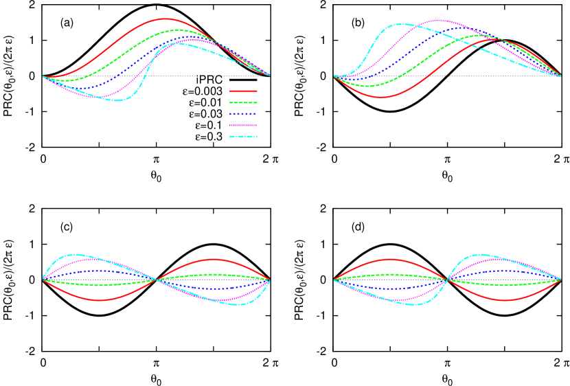
Figure 2: The same as Fig. 1 with $r=0.99$.

The comparison of the PRCs in this comment with the corresponding $Q$ functions in Fig. 2 of Ref. Pazó and Gallego (2020) evidences that $Q(\theta,A)$ is not simply the PRC. Indeed, $Q$ in (2) has only the first harmonic in $\theta$, whereas the non-infinitesimal PRCs in the figures display additional Fourier components. In spite of these dissimilarities, simple visual inspection indicates that the PRC strongly resembles the coupling function $Q$ in all four cases. For example, we observe the same loss of non-negativeness of the (type-I) iPRC as $A$ increases in panel (a), or the transition from a synchronizing iPRC to a desynchronizing PRC for large enough $A$ in panel (c). Summarizing, our simulations confirm that the main attributes of the coupling function $Q$ are shared by the non-infinitesimal PRC.

REFERENCES

References

- Pazó and Gallego (2020) D. Pazó and R. Gallego, “The Winfree model with non-infinitesimal phase-response curve: Ott-Antonsen theory,” Chaos 30, 073139 (2020).
- Winfree (1967) A. T. Winfree, “Biological rhythms and the behavior of populations of coupled oscillators.” J. Theor. Biol. 16, 15–42 (1967).
- Winfree (1980) A. T. Winfree, The Geometry of Biological Time (Springer, New York, 1980).
- Rosenblum and Pikovsky (2019) M. Rosenblum and A. Pikovsky, “Numerical phase reduction beyond the first order approximation,” Chaos 29, 011105 (2019).
- León and Pazó (2019) I. León and D. Pazó, “Phase reduction beyond the first order: The case of the mean-field complex Ginzburg-Landau equation,” Phys. Rev. E 100, 012211 (2019).
- Izhikevich (2007) E. M. Izhikevich, Dynamical Systems in Neuroscience (The MIT Press, Cambridge, Massachusetts, 2007) Chap. 10.