Abstract. Motivated by the complexity of network data, we propose a directed hybrid random network that mixes preferential attachment (PA) rules with uniform attachment (UA) rules. When a new edge is created, with probability $p\in[0,1]$, it follows the PA rule. Otherwise, this new edge is added between two uniformly chosen nodes. Such mixture makes the in- and out-degrees of a fixed node grow at a slower rate, compared to the pure PA case, thus leading to lighter distributional tails. Under this hybrid model, however, existing inference methods (cf. [31]) become inapplicable. Instead, we develop alternative approaches which are then applied to both synthetic and real datasets. We see that with extra flexibility given by the parameter $p$, the hybrid random network provides a better fit to real-world scenarios, where lighter tails from in- and out-degrees are observed.

AMS subject classifications.

Primary: 05C80; 62G32

Secondary: 05C07

Key words. Preferential attachment; uniform attachment; in- and out-degrees; power laws; random networks

1. Introduction

The preferential attachment (PA) mechanism [4] has been widely used to model interactions or communications among the entities in a network-based system, especially evolving networks. A precursory study of PA networks was conducted by de Sollar Price [29] to model the growth of citation networks, where the research outcome coincides with a sociological theory called the Matthew Effect [20], inducing a well known economic manifestation—“The rich get richer; the poor get poorer”.

One of the most appealing properties of the PA network is scale-free (i.e., the node degree distribution follows a power law), rendering that the PA rule has become an attractive choice for real network modeling, such as the World Wide Web [15] and collaboration networks [23]. We refer the readers to Durrett [10], van der Hofstad [30] for some text-style elaborations of the elementary descriptions and probabilistic properties of PA networks. Recent studies have extended classical PA networks to directed counterparts, where some asymptotic theories [34, 32, 33] and the maximum likelihood estimators (MLEs) of the parameters [31] have been developed. Other recent works on the mathematical treatments of PA networks and their variants include Gao and van der Vaart [11], Alves et al. [1], Mahmoud [18], Wang and Resnick [35], Zhang and Mahmoud [36].

However, classical (either directed or undirected) PA networks do not always fit the real network data well, nor are they able to precisely capture some key attributes of the networks. Alternatively, Atalay et al. [2] proposed a model mixing PA and uniform attachment (UA) to investigate the buyer-supplier network in the United States, showing that the proposed model has outperformed the pure PA model. In this paper, we consider a class of directed hybrid random networks (HRNs) presenting PA and UA mechanisms simultaneously, governed by a tuning parameter $p\in[0,1]$. The presence of UA in the proposed model effectively leverages the heavy tail produced by the PA mechanism, rendering that the model tentatively better fits the real networks whose degree distributions are less heavier.

Note that by [8], an undirected sublinear PA model with attachment probability proportional to $\text{Degree}_{v}^{\alpha}$, $\alpha\in(0,1)$, produces a degree distribution with stretched exponential tails,

$$\exp(-k^{\alpha}),\qquad\alpha\in(0,1),\qquad\text{fro k large},$$

which is lighter than the power-law tail. With a stretched exponential tails, widely adopted methods, e.g. [6], may provide inaccurate tail estimates, since the underlying distributional tail deviates from power laws; see [9] for a detailed discussion. Therefore, in this paper, we restrict ourselves to the mixture of PA and UA schemes to obtain a lighter tail of the degree distribution and retain the asymptotic power-law behavior simultaneously.

In the literature, there is a limited amount of work on the random structures that integrate PA and UA during the evolution. Shao et al. [26] carried out a simulation study of the degree distribution in a standard mixed attachment growing network. More recently, [24] investigated the scale-free property of the degree distribution in an analogous model through recursive formulations. We describe the construction of a hybrid random network in Section 2, and study theoretical properties of its degree distributions in Section 3. We then propose estimation methods and explore properties of the estimators in Section 4, which facilitate the numerical studies on both synthetic datasets (cf. Section 5) and real network data (cf. Section 6). With all results available, we also provide some interesting direction for future research in Section 7.

2. Hybrid Random Networks

Let $\mathcal{H}_{n}(V_{n},E_{n};\alpha,\beta,\gamma,p,\delta_{\rm in},\delta_{\rm out})$ denote the structure of a class of HRNs consisting of a vertex set $V_{n}$ and an edge set $E_{n}$ at time $n$, parameterized by a set of parameters $\bm{\theta}:=(\alpha,\beta,\gamma,p,\delta_{\rm in},\delta_{\rm out})$ subject to $\alpha+\beta+\gamma=1$, $\delta_{\rm in},\delta_{\rm out}>0$. Specifically, the parameters, $\alpha$, $\beta$ and $\gamma$, represent the probabilities of presenting one of the three edge-creation scenarios at each step. With probability $\alpha$, there emerges a directed edge from the newcomer to an existing node. With probability $\gamma$, there emerges a directed edge from an existing node to the newcomer. With probability $\beta=1-\alpha-\gamma$, a directed edge is added between two existing nodes. See Figure 1 for a graphical illustration.

Figure 1. Three edge-addition scenarios respectively corresponding to $\alpha$, $\beta$ and $\gamma$ (from left to right)

The offset parameters $\delta_{\rm in}$ and $\delta_{\rm out}$ respectively control the growth rate of in-degree and out-degree in the network. Another parameter $0\leq p\leq 1$ specifies the probability of executing PA when sampling the node(s) at the end(s) of the newly added edge at each timestamp. The functionality of $p$ is to balance PA and UA in the model, and accordingly the proposed HRN becomes more flexible than pure PA network model for characterizing the in-degree and out-degree tail distributions of real network data.

We start the network with $\mathcal{H}_{0}$, which is a self-looped single node labeled with $1$. At any subsequent point $n\geq 1$, flip a three-sided coin, for which the probabilities of landing the three faces up are respectively $\alpha$ (associated with scenario 1), $\beta$ (associated with scenario 2) and $\gamma$ (associated with scenario 3). Let $J_{n}\in\{1,2,3\}$ indicate the occurrence of the scenario type at time $n$, i.e. $J_{n}$ is a tri-nomial random variable on $\{1,2,3\}$ with cell probability $\alpha$, $\beta$ and $\gamma$, respectively. The network evolves as below.

1. For $J_{n}=1$, we add a new node $u$ to the network, connecting it to an existing node $i\in V_{n-1}$ by a directed edge pointing to $i$ with probability

   $$p\times\frac{D^{\rm in}_{i}(n-1)+\delta_{\rm in}}{\sum_{k\in V_{n-1}}(D^{\rm in}_{k}(n-1)+\delta_{\rm in})}+(1-p)\times\frac{1}{|V_{n-1}|},$$ (1)

   where $D^{\rm in}_{i}(n)$ is the in-degree of $i$ in $\mathcal{H}_{n}$, and $|V_{n}|$ denotes the number of nodes at time $n$.

2. For $J_{n}=2$, we add a directed edge between two existing nodes $i,j\in V_{n-1}$, where $i$ and $j$ are sampled independently. Suppose that the newly added edge is pointed (from $j$) to $i$, then the associated probability is given by

   $$\left(p\times\frac{D^{\rm out}_{j}(n-1)+\delta_{\rm out}}{\sum_{k\in V_{n-1}}(D^{\rm out}_{k}(n-1)+\delta_{\rm out})}+(1-p)\times\frac{1}{|V_{n-1}|}\right)$$

   $$\qquad{}\times\left(p\times\frac{D^{\rm in}_{i}(n-1)+\delta_{\rm in}}{\sum_{k\in V_{n-1}}(D^{\rm in}_{k}(n-1)+\delta_{\rm in})}+(1-p)\times\frac{1}{|V_{n-1}|}\right),$$ (2)

   where $D^{\rm out}_{i}(n)$ is analogously defined as the out-degree of node $i$ in $\mathcal{H}_{n}$. Note that no new node is added to the network under this scenario, hence $V_{n}=V_{n-1}$. Besides, there is a positive probability that a node is sampled twice; If so, a self loop is created.

3. For $J_{n}=3$, a new node $u$ is appended to the network by a directed edge emanating out from $j\in V_{n-1}$ with probability

   $$p\times\frac{D^{\rm out}_{j}(n-1)+\delta_{\rm out}}{\sum_{k\in V_{n-1}}(D^{\rm out}_{k}(n-1)+\delta_{\rm out})}+(1-p)\times\frac{1}{|V_{n-1}|}.$$ (3)

Some simplifications can be made to the conditional probabilities in Equations (1), (2) and (3) after observing $\sum_{k\in V_{n-1}}(D^{\rm in}_{k}(n-1)+\delta_{\rm in})=n+\delta_{\rm in}|V_{n-1}|$ and $\sum_{k\in V_{n-1}}(D^{\rm out}_{k}(n-1)+\delta_{\rm out})=n+\delta_{\rm out}|V_{n-1}|$ (since our initial time is $n=0$). Meanwhile, the fact that the two fractions have different denominators in each of the conditional probabilities would have brought a great deal of challenges to both analytical computations and parameter estimations.

3. Degree Distribution

In this section, we investigate the in-degree and out-degree distributions of $\mathcal{H}_{n}$. Let $\mathcal{F}_{n}$ be the sigma field generated by the evolution of a hybrid random network up to time $n$, i.e., $\{\mathcal{H}_{k}:k\leq n\}$. According to the evolutionary scenarios described in Section 2, we have for $i\in V_{n}$,

$$\mathbb{P}\left(D^{\rm in}_{i}(n+1)-D^{\rm in}_{i}(n)=1\,|\,\mathcal{F}_{n}\right)$$

$$\qquad{}=(\alpha+\beta)\left[\frac{p\left(D^{\rm in}_{i}(n)+\delta_{\rm in}\right)}{\sum_{k\in V_{n}}\left(D^{\rm in}_{k}(n)+\delta_{\rm in}\right)}+\frac{(1-p)}{|V_{n}|}\right],$$ (4)

$$\mathbb{P}\left(D^{\rm out}_{i}(n+1)-D^{\rm out}_{i}(n)=1\,|\,\mathcal{F}_{n}\right)$$

$$\qquad{}=(\beta+\gamma)\left[\frac{p\left(D^{\rm out}_{i}(n)+\delta_{\rm out}\right)}{\sum_{k\in V_{n}}\left(D^{\rm out}_{k}(n)+\delta_{\rm out}\right)}+\frac{(1-p)}{|V_{n}|}\right].$$ (5)

We present important theoretical results on the in- and out-degree sequences in an HRN. Relevant proofs of the theorems in this section are collected in Appendices A, B and C.

3.1. Expected In- and Out-Degrees

The next theorem specifies the growth rates of $\mathbb{E}\left[D^{\rm in}_{i}(n)\right]$ and $\mathbb{E}\left[D^{\rm out}_{i}(n)\right]$ for a fixed node $i\in V_{n}$.

Theorem 1.

There exist $M_{1},M_{2}>0$ such that

$$\sup_{i\geq 1}\frac{\mathbb{E}\left[D^{\rm in}_{i}(n)\right]}{n^{C_{1}}}\leq M_{1}\qquad\mbox{and}\qquad\sup_{i\geq 1}\frac{\mathbb{E}\left[D^{\rm out}_{i}(n)\right]}{n^{C_{2}}}\leq M_{2},$$

where $C_{1}$ and $C_{2}$ are respectively given by

$$C_{1}=\frac{(\alpha+\beta)p}{1+\delta_{\rm in}(1-\beta)}\qquad\mbox{and}\qquad C_{2}=\frac{(\beta+\gamma)p}{1+\delta_{\rm out}(1-\beta)}.$$

It is worth noting that the growth rates $C_{1}$ and $C_{2}$ are smaller than those in a pure directed PA model (i.e., $p=1$). This suggests that incorporating a non-negligible number of uniformly added edges creates lighter distributional tails for both in- and out-degrees.

3.2. Almost Sure Convergence of the In- and Out-Degrees

Next, we study the asymptotic properties of $D^{\rm in}_{i}(n)$ and $D^{\rm out}_{i}(n)$ by utilizing martingale formulations [10, Chapter 4]. By the conditional probability in Equation (4), we have for $i\in V_{n}$,

$$\mathbb{P}\left(D^{\rm in}_{i}(n+1)-D^{\rm in}_{i}(n)=1\,|\,\mathcal{F}_{n}\right)\geq\frac{p\left(D^{\rm in}_{i}(n)+\delta_{\rm in}\right)(\alpha+\beta)}{1+n+\delta_{\rm in}|V_{n}|},$$

which implies that for a fixed $i$,

$$M^{\rm in}_{n+1}:=\frac{D^{\rm in}_{i}(S_{i}+n+1)+\delta_{\rm in}}{\prod_{k=0}^{n}\left(1+\frac{p(\alpha+\beta)}{S_{i}+k+1+\delta_{\rm in}|V_{S_{i}+k}|}\right)}$$ (6)

is a sub-martingale with respect to the filtration $(\mathcal{F}_{n})_{n\geq 0}$, where $S_{i}:=\inf\{n\geq 0:|V_{n}|=i\}$. Analogously, based on Equation (5), we construct another sub-martingale sequence for out-degrees:

$$M^{\rm out}_{n+1}:=\frac{D^{\rm out}_{i}(S_{i}+n+1)+\delta_{\rm out}}{\prod_{k=0}^{n}\left(1+\frac{p(\beta+\gamma)}{S_{i}+k+1+\delta_{\rm out}|V_{S_{i}+k}|}\right)}.$$ (7)

In the proof of Theorem 3, we specify the asymptotic orders of the denominator in Equation (6) (a similar argument also applies to the denominator in Equation (7)). Then applying the martingale convergence theorem [10, Theorem 4.2.11] gives the following convergence results for the in- and out-degrees of a fixed node. Details of the proof of Theorem 2 are given in Appendix B.

Theorem 2.

For a fixed node $i$, there exist finite random variables $\zeta_{i}$ and $\xi_{i}$ such that as $n\to\infty$,

$$\left(\frac{D^{\rm in}_{i}(n)}{n^{C_{1}}},\frac{D^{\rm out}_{i}(n)}{n^{C_{2}}}\right)\,\overset{a.s.}{\longrightarrow}\,\left(\zeta_{i},\xi_{i}\right),$$

where $C_{1}$ and $C_{2}$ are identical to those developed in Theorem 1.

3.3. Expected Degree Counts

In addition, we develop the asymptotics for $N_{m}^{\rm in}(n)/n$, and $N_{m}^{\rm out}(n)/n$, $m\geq 0$, i.e., the empirical proportional of nodes with in- or out-degree $m$ in $\mathcal{H}_{n}$. Let ${\rm NB}(n,q)$ represent a negative binomial random variable with generating function

$$(s+(1-s)/q)^{-n},\qquad s\in[0,1].$$

Theorem 3.

Define $\tilde{\delta}_{\rm in}:=\delta_{\rm in}/p+(1-p)/\bigl{(}p(1-\beta)\bigr{)}$ and $\tilde{\delta}_{\rm out}:=\delta_{\rm out}/p+(1-p)/\bigl{(}p(1-\beta)\bigr{)}$. Let ${\rm NB}(\tilde{\delta}_{\rm in},p_{1})$, ${\rm NB}(1+\tilde{\delta}_{\rm in},p_{1})$, ${\rm NB}(\tilde{\delta}_{\rm out},p_{2})$ and ${\rm NB}(1+\tilde{\delta}_{\rm out},p_{2})$, be four independent negative binomial random variables, and set $T_{\rm in}$ and $T_{\rm out}$ to be two independent exponential random variables with rates

$$\frac{1+\delta_{\rm in}(1-\beta)}{p(\alpha+\beta)}\qquad\text{and}\qquad\frac{1+\delta_{\rm out}(1-\beta)}{p(\beta+\gamma)},$$

respectively (which are also independent from ${\rm NB}(\tilde{\delta}_{\rm in},p_{1})$, ${\rm NB}(1+\tilde{\delta}_{\rm in},p_{1})$, ${\rm NB}(\tilde{\delta}_{\rm out},p_{2})$ and ${\rm NB}(1+\tilde{\delta}_{\rm out},p_{2})$). As $n\to\infty$, we have

$$\frac{N_{m}^{\rm in}(n)}{n}\stackrel{{\scriptstyle p}}{{\longrightarrow}}\tilde{\psi}_{m}^{\rm in}\qquad\text{and}\qquad\frac{N_{m}^{\rm out}(n)}{n}\stackrel{{\scriptstyle p}}{{\longrightarrow}}\tilde{\psi}_{m}^{\rm out},$$

where

$$\tilde{\psi}_{m}^{\rm in} ={\alpha}\,\mathbb{P}\left({\rm NB}\left(\tilde{\delta}_{\rm in},e^{-T_{\rm in}}\right)=m\right)$$

$$\qquad{}+{\gamma}\,\mathbb{P}\left(1+{\rm NB}\left(1+\tilde{\delta}_{\rm in},e^{-T_{\rm in}}\right)=m\right),$$ (8)

$$\tilde{\psi}_{m}^{\rm out} ={\alpha}\,\mathbb{P}\left({\rm NB}\left(\tilde{\delta}_{\rm out},e^{-T_{\rm out}}\right)=m\right)$$

$$\qquad{}+{\gamma}\,\mathbb{P}\left(1+{\rm NB}\left(1+\tilde{\delta}_{\rm out},e^{-T_{\rm out}}\right)=m\right).$$ (9)

We conclude this section by remarking that the limit functions in Equations (8) and (9) coincide with those from a pure PA network with parameters $(\alpha,\beta,\gamma,\tilde{\delta}_{\text{in}},\tilde{\delta}_{\text{out}}).$ In fact, when $\beta=0$, the HRN is identical to a pure PA network with $(\alpha,0,\gamma,\tilde{\delta}_{\text{in}},\tilde{\delta}_{\text{out}})$, where all established results for the pure PA model can be readily applied. The major goal in the proof of Theorem 3 is to show that the discrepancy caused by having random number of edges is negligible when $n$ is large.

4. Parameter Estimation

In this section, we propose our estimation scheme for the parameters in the HRN model described in Section 2, under a few regularity conditions given as follows. We assume the evolution history of the entire network is available since the beginning, recorded in the edge list $\bm{E}:=\{E_{k}\}_{k=0}^{n-1}$, where $E_{0}=(1,1)$ is deterministic. Notice that $\gamma=1-(\alpha+\beta)$ completely depends on $\alpha$ and $\beta$ so that the model is parametrized in terms of $(\alpha,\beta,p,\delta_{\rm in},\delta_{\rm out})$. We also assume $0\leq p\leq 1$, $0\leq\alpha,\beta<1$ and $0<\alpha+\beta\leq 1$, where the latter two jointly ensure the exclusion of the trivial cases of either $\alpha$, $\beta$ or $\gamma$ taking value $1$. The offset parameters $\delta_{\rm in}$ and $\delta_{\rm out}$ are assumed to be positive and finite.

4.1. Maximum Likelihood Estimation

In a slight abuse of notation, let $E_{k}=(v_{k,1},v_{k,2})$ represent the edge (from $v_{k,1}$ to $v_{k,2}$) added at time $k$, $v_{k,1}$ and $v_{k,2}$ can be the nodes from the existing network or newcomers. According to Equations (1), (2) and (3), the likelihood of the model is given by

$$L(\bm{\theta}\,|\,\bm{E}) =\prod_{k=1}^{n}\left[\alpha\left(\frac{p(D^{\rm in}_{v_{k,2}}(k-1)+\delta_{\rm in})}{k+\delta_{\rm in}|V_{k-1}|}+\frac{1-p}{|V_{k-1}|}\right)\right]^{\mathbb{I}_{\{J_{k}=1\}}}$$

$$\qquad{}\times\prod_{k=1}^{n}\left[\beta\left(\frac{p(D^{\rm out}_{v_{k,1}}(k-1)+\delta_{\rm out})}{k+\delta_{\rm out}|V_{k-1}|}+\frac{1-p}{|V_{k-1}|}\right)\right.$$

$$\qquad{}\qquad{}\times\left.\left(\frac{p(D^{\rm in}_{v_{k,2}}(k-1)+\delta_{\rm in})}{k+\delta_{\rm in}|V_{k-1}|}+\frac{1-p}{|V_{k-1}|}\right)\right]^{\mathbb{I}_{\{J_{k}=2\}}}$$

$$\qquad{}\times\prod_{k=1}^{n}\left[(1-\alpha-\beta)\left(\frac{p(D^{\rm out}_{v_{k,1}}(k-1)+\delta_{\rm out})}{k+\delta_{\rm out}|V_{k-1}|}+\frac{1-p}{|V_{k-1}|}\right)\right]^{\mathbb{I}_{\{J_{k}=3\}}},$$

then the log-likelihood becomes

$$\log L(\bm{\theta}\,|\,\bm{E})$$

$$\quad{}=\log\alpha\sum_{k=1}^{n}\mathbb{I}_{\{J_{k}=1\}}+\log\beta\sum_{k=1}^{n-1}\mathbb{I}_{\{J_{k}=2\}}+\log(1-\alpha-\beta)\sum_{k=2}^{n}\mathbb{I}_{\{J_{k}=3\}}$$

$$\qquad{}+\sum_{k=1}^{n}\log\left[\bigl{(}pD^{\rm in}_{v_{k,2}}(k-1)+\delta_{\rm in}\bigr{)}|V_{k-1}|+(1-p)k\right]\mathbb{I}_{\{J_{k}=\{1,2\}\}}$$

$$\qquad{}+\sum_{k=1}^{n}\log\left[\bigl{(}pD^{\rm out}_{v_{k,1}}(k-1)+\delta_{\rm out}\bigr{)}|V_{k-1}|+(1-p)k\right]\mathbb{I}_{\{J_{k}=\{2,3\}\}}$$

$$\qquad{}-\sum_{k=1}^{n}\log\left[k|V_{k-1}|+|V_{k-1}|^{2}\delta_{\rm in}\right]\mathbb{I}_{\{J_{k}=\{1,2\}\}}$$

$$\qquad{}-\sum_{k=1}^{n}\log\left[k|V_{k-1}|+|V_{k-1}|^{2}\delta_{\rm out}\right]\mathbb{I}_{\{J_{k}=\{2,3\}\}},$$

from which we see that the score functions of $\alpha$ and $\beta$ are independent of those of the other parameters.

Carrying out an analogous analysis as in [31, Section 3.1], we find that the MLEs for $\alpha$ and $\beta$ are respectively given by

$$\hat{\alpha}^{\,\rm MLE}=\frac{1}{n}\sum_{k=1}^{n}\mathbb{I}_{\{J_{k}=1\}}\qquad\text{and}\qquad\hat{\beta}^{\,\rm MLE}=\frac{1}{n}\sum_{k=1}^{n}\mathbb{I}_{\{J_{k}=2\}}.$$

To develop the MLEs for $\delta_{\rm in}$, $\delta_{\rm out}$ and $p$, we calculate their score functions to get

$$\frac{\partial}{\partial\delta_{\rm in}}\log L(\bm{\theta}\,|\,\bm{E}) =\sum_{k=1}^{n}\frac{|V_{k-1}|}{\bigl{(}pD^{\rm in}_{v_{k,2}}(k-1)+\delta_{\rm in}\bigr{)}|V_{k-1}|+(1-p)k}\,\mathbb{I}_{\{J_{k}=\{1,2\}\}}$$

$$\qquad{}-\sum_{k=1}^{n}\frac{|V_{k-1}|}{k+|V_{k-1}|\delta_{\rm in}}\,\mathbb{I}_{\{J_{k}=\{1,2\}\}},$$ (10)

$$\frac{\partial}{\partial\delta_{\rm out}}\log L(\bm{\theta}\,|\,\bm{E}) =\sum_{k=1}^{n}\frac{|V_{k-1}|}{\bigl{(}pD^{\rm out}_{v_{k,1}}(k-1)+\delta_{\rm out}\bigr{)}|V_{k-1}|+(1-p)k}\,\mathbb{I}_{\{J_{k}=\{2,3\}\}}$$

$$\qquad{}-\sum_{k=1}^{n}\frac{|V_{k-1}|}{k+|V_{k-1}|\delta_{\rm out}}\,\mathbb{I}_{\{J_{k}=\{2,3\}\}},$$ (11)

$$\frac{\partial}{\partial p}\log L(\bm{\theta}\,|\,\bm{E}) =\sum_{k=1}^{n}\frac{\bigl{(}D^{\rm in}_{v_{k,2}}(k-1)|V_{k-1}|-k\bigr{)}\mathbb{I}_{\{J_{k}=\{1,2\}\}}}{\bigl{(}pD^{\rm in}_{v_{k,2}}(k-1)+\delta_{\rm in}\bigr{)}|V_{k-1}|+(1-p)k}$$

$$\qquad{}+\sum_{k=1}^{n}\frac{\bigl{(}D^{\rm out}_{v_{k,1}}(k-1)|V_{k-1}|-k\bigr{)}\mathbb{I}_{\{J_{k}=\{2,3\}\}}}{\bigl{(}pD^{\rm out}_{v_{k,1}}(k-1)+\delta_{\rm out}\bigr{)}|V_{k-1}|+(1-p)k}.$$ (12)

We proceed by first setting (10) to 0. Note that due to the randomness of $|V_{k-1}|$, the methodology given in [31] is not directly applicable. Instead, we approximate the score function (10) as follows.

$$\sum_{k=1}^{n} \frac{|V_{k-1}|}{\bigl{(}pD^{\rm in}_{v_{k,2}}(k-1)+\delta_{\rm in}\bigr{)}|V_{k-1}|+(1-p)k}\,\mathbb{I}_{\{J_{k}=\{1,2\}\}}$$

$$=\sum_{k=1}^{n}\frac{\mathbb{I}_{\{J_{k}=\{1,2\}\}}}{\bigl{(}pD^{\rm in}_{v_{k,2}}(k-1)+\delta_{\rm in}\bigr{)}+(1-p)k/|V_{k-1}|}$$

$$=\frac{1}{p}\sum_{k=1}^{n}\frac{\mathbb{I}_{\{J_{k}=\{1,2\}\}}}{D^{\rm in}_{v_{k,2}}(k-1)+\tilde{\delta}_{\text{in}}}+R_{\text{in}}(n),$$

where

$$R_{\text{in}}(n)=$$

$$\sum_{k=1}^{n}\frac{\mathbb{I}_{\{J_{k}=\{1,2\}\}}}{p}\left(\frac{1}{D^{\rm in}_{v_{k,2}}(k-1)+\delta_{\rm in}/p+(1-p)k/|V_{k-1}|}-\frac{1}{D^{\rm in}_{v_{k,2}}(k-1)+\tilde{\delta}_{\text{in}}}\right).$$

Therefore,

$$|R_{\text{in}}(n)| \leq\frac{1}{p}\sum_{k=1}^{n}\frac{(1-p)/p\left|k/|V_{k-1}|-1/(1-\beta)\right|\mathbb{I}_{\{J_{k}=\{1,2\}\}}}{(D^{\rm in}_{v_{k,2}}(k-1)+\delta_{\rm in}/p+(1-p)k/|V_{k-1}|)(D^{\rm in}_{v_{k,2}}(k-1)+\tilde{\delta}_{\text{in}})}$$

$$\leq\frac{1-p}{p^{2}}\sum_{k=1}^{n}\frac{|k/|V_{k-1}|-1/(1-\beta)|}{(\delta_{\rm in}/p+(1-p)k/|V_{k-1}|)\tilde{\delta}_{\text{in}}}.$$

Since $|V_{n-1}|/n\,\overset{a.s.}{\longrightarrow}\,1/(1-\beta)$, then by the Cesàro convergence of random variables, we have $|R_{\text{in}}(n)|/n\,\overset{a.s.}{\longrightarrow}\,0$. Then the approximate score equation in (10) becomes

$$\frac{1}{n}\sum_{k=1}^{n}\frac{\mathbb{I}_{\{J_{k}=\{1,2\}\}}}{D^{\rm in}_{v_{k,2}}(k-1)+\tilde{\delta}_{\text{in}}} =\frac{1}{n}\sum_{k=1}^{n}\frac{|V_{k-1}|}{k+|V_{k-1}|\delta_{\rm in}}\,\mathbb{I}_{\{J_{k}=\{1,2\}\}}.$$

Applying the method in [31] further yields the following approximate score function:

$$\sum_{m=0}^{\infty}\frac{N^{\text{in}}_{>m}(n)/n}{m+\tilde{\delta}_{\text{in}}} =\frac{\gamma}{\tilde{\delta}_{\text{in}}}+\frac{(\alpha+\beta)(1-\beta)}{1+\delta_{\rm in}(1-\beta)},$$ (13)

where $N^{\text{in}}_{>m}(n)$ denotes the number of nodes with in-degree strictly greater than $m$ in $\mathcal{H}_{n}$.

Similarly, the score equation with respect to (11) can be approximated by

$$\sum_{m=0}^{\infty}\frac{N^{\text{out}}_{>m}(n)/n}{m+\tilde{\delta}_{\text{out}}} =\frac{\alpha}{\tilde{\delta}_{\text{out}}}+\frac{(\beta+\gamma)(1-\beta)}{1+\delta_{\rm out}(1-\beta)},$$ (14)

with $N^{\text{out}}_{>m}(n)$ being the number of nodes with out-degree strictly greater than $m$ in $\mathcal{H}_{n}$. However, with (13) and (14) available, the approximation to the third score equation in (12) leads to a deterministic solution of $p=1$. This indicates standard approaches to find MLE as in [31] are not able to give us the desirable results. Alternatively, in the next section, we formulate the MLE searching procedure as a nonlinear optimization problem with constraint $p\in[0,1]$.

4.2. Nonlinear optimization

Having seen that standard ways to find MLE by solving score equations do not produce reasonable estimates, we consider the MLE-searching procedure as a nonlinear optimization problem with properly identified constraints such that $\alpha,\beta,p\in[0,1]$ and $\delta_{\rm in},\delta_{\rm out}>0$. Specifically, we adopt the Nelder-Mead (N-M) algorithm proposed by Nelder and Mead [22]. The N-M algorithm is appealing for efficiency as it usually converges within a relatively small number of iterations. Despite limited knowledge about the theoretical results of the N-M algorithm [16], its utilization is widespread in the community since it generally performs well in practice. One practical issue of the algorithm is that its convergence is quite sensitive to the choice of the initial simplex. An improper initial simplex has become the main cause of the algorithm breakdown.

Having this in mind, we back up with an alternative — a Bayesian estimation based on Markov chain Monte Carlo (MCMC) algorithms. Specifically, we consider a Metropolis-Hastings (M-H) algorithm [21, 14]. Being a classical approach, the fundamentals of the M-H algorithms have been extensively elaborated in a wide range of texts, such as Chen et al. [5], Liang et al. [17], Gelman et al. [12]. Here we only present a few essential steps.

Let $\pi(\bm{\theta};\bm{\psi})$ be the prior distribution of $\bm{\theta}$, where $\bm{\psi}$ is a collection of hyper-parameters. Under this setting, the likelihood function $L(\bm{\theta}\,|\,\bm{E})$ is the posterior distribution of $\bm{\theta}$. As it is difficult to sample $\bm{\theta}$ from this posterior distribution directly, the M-H algorithm generates a Markov process whose stationary distribution is the same as the posterior distribution, and the generation of the process is done in an iterative manner. Let $\bm{\theta}^{(t)}$ be the estimates from the $t$-th iteration, and let $Q(\bm{\theta}^{\rm prop}\,|\,\bm{\theta}^{(t)})$ denote the proposal density governing the transition probability from the current estimates to a proposed set of candidates. Suppose that the distribution $Q$ is symmetric, then the acceptance rate $a(\bm{\theta}^{\rm prop}\,|\,\bm{\theta}^{(t)})$ is given by

$$a(\bm{\theta}^{\rm prop}\,|\,\bm{\theta}^{(t)}) =\min\left\{\frac{L(\bm{\theta}^{\rm prop}\,|\,\bm{E})Q(\bm{\theta}^{\rm prop}\,|\,\bm{\theta}^{(t)})}{L(\bm{\theta}^{(t)}\,|\,\bm{E})Q(\bm{\theta}^{(t)}\,|\,\bm{\theta}^{\rm prop})},1\right\}$$

$$=\min\left\{\frac{L(\bm{\theta}^{\rm prop}\,|\,\bm{E})}{L(\bm{\theta}^{(t)}\,|\,\bm{E})},1\right\}.$$

This can be done by generating a standard uniform random variable $U$ such that $\bm{\theta}^{(t+1)}=\bm{\theta}^{\rm prop}$ if $U<a(\bm{\theta}^{\rm prop}\,|\,\bm{\theta}^{(t)})$; $\bm{\theta}^{(t+1)}=\bm{\theta}^{(t)}$, otherwise.

There are multiple ways of selecting an appropriate proposal distribution $Q(\bm{\theta}^{\rm prop}\,|\,\bm{\theta}^{(t)})$, where a simple approach based on random walk is adopted. Consider $\bm{\theta}^{\rm prop}=\bm{\theta}^{(t)}+\bm{\epsilon}$, where $\bm{\epsilon}$ is a random variable for step size. Note that the conditional distribution $Q(\bm{\theta}^{\rm prop}\,|\,\bm{\theta}^{(t)})$ is fully specified by the distribution of $\bm{\epsilon}$. Thus, we only need to choose a symmetric distribution for $\bm{\epsilon}$ to satisfy the required condition, such as normal or uniform distribution. One drawback of MCMC algorithms is the lack of theoretical foundation for the assessment of convergence. Since the initial samples of $\bm{\theta}$ from the prior distribution may fall into a low density of the target posterior distribution, a sufficiently large burn-in period is always necessary. The number of iterations needed for the algorithm to converge is closely related to its convergence rate [19], which is practically unwieldy in general. Here we will rely on a few widely-accepted graphical diagnostics to assess the convergence of MCMC algorithms, such as time-series plots and running mean plots [27].

5. Simulations

In this section, we carry out an extensive simulation study along with a sensitivity analysis for the estimation of the parameters for HRNs. We focus on the performance of the N-M and M-H algorithms under different combinations of $(\alpha,\beta,p)$. Specifically, we consider $p\in\{0.8,0.6,0.2\}$ (respectively corresponding to dominant PA, roughly even PA and UA and dominant UA) paired with $(\alpha,\beta)\in\{(0.8,0.1),(0.45,0.1),(0.1,0.8)\}$. The other two offset parameters are set to be $\delta_{\rm in}=1.3$ and $\delta_{\rm out}=0.7$.

For each setting, we generate $R=100$ replicates of independent HRNs with $n=10,000$ edges. When applying the M-H algorithm, we use non-informative priors. The burn-in number is set to be 10,000, and the number of iterations after burn-in is 20,000. To avoid auto-correlation in the posterior sample, a thinning sampling of gap 500 is used. In Tables 1, 2 and 3, we present the point estimates, the absolute percentages of bias and the standard errors based on the simulation results.

Table 1. Simulation results with large $p=0.8$.

		Nelder-Mead Algorithm					Metropolis-Hastings Algorithm
Parameters		$\hat{\alpha}$	$\hat{\beta}$	$\hat{p}$	$\hat{\delta}_{\rm in}$	$\hat{\delta}_{\rm out}$	$\hat{\alpha}$	$\hat{\beta}$	$\hat{p}$	$\hat{\delta}_{\rm in}$	$\hat{\delta}_{\rm out}$
$\alpha=0.1$	Est.	0.0996	0.8004	0.7908	1.2304	0.6345	0.0997	0.8002	0.8183	1.4513	0.8331
$\beta=0.8$	Bias(%)	0.4068	0.0534	1.1653	5.6584	10.3172	0.2669	0.0201	2.2357	10.4235	15.9719
$p=0.8$	S.E.	0.0003	0.0004	0.0010	0.0103	0.0058	0.0003	0.0004	0.0079	0.0640	0.0567
$\alpha=0.8$	Est.	0.8003	0.0999	0.7611	1.1776	0.6251	0.8001	0.1000	0.8128	1.3351	0.8302
$\beta=0.1$	Bias(%)	0.0359	0.1087	5.1091	10.3971	11.9915	0.0118	0.0231	1.5728	2.6264	15.6826
$p=0.8$	S.E.	0.0004	0.0003	0.0048	0.0154	0.0138	0.0004	0.0003	0.0118	0.0361	0.0449
$\alpha=0.45$	Est.	0.4497	0.1003	0.8153	1.3608	0.7339	0.4494	0.1005	0.8305	1.4193	0.7714
$\beta=0.1$	Bias(%)	0.0763	0.3218	1.8762	4.6677	4.6199	0.1397	0.4989	3.6774	8.4022	9.2520
$p=0.8$	S.E.	0.0005	0.0003	0.0049	0.0156	0.0113	0.0005	0.0003	0.0098	0.0324	0.0236

Table 2. Simulation results with moderate $p=0.6$.

		Nelder-Mead Algorithm					Metropolis-Hastings Algorithm
Parameters		$\hat{\alpha}$	$\hat{\beta}$	$\hat{p}$	$\hat{\delta}_{\rm in}$	$\hat{\delta}_{\rm out}$	$\hat{\alpha}$	$\hat{\beta}$	$\hat{p}$	$\hat{\delta}_{\rm in}$	$\hat{\delta}_{\rm out}$
$\alpha=0.1$	Est.	0.1002	0.7996	0.6001	1.3340	0.7012	0.1003	0.7995	0.6216	1.5576	0.9057
$\beta=0.8$	Bias(%)	0.2090	0.0529	0.0101	2.5520	0.1694	0.3223	0.0645	3.4725	16.5359	22.7067
$p=0.6$	S.E.	0.0003	0.0004	0.0016	0.0162	0.0134	0.0003	0.0005	0.0077	0.0819	0.0704
$\alpha=0.8$	Est.	0.8002	0.1001	0.5713	1.1725	0.6319	0.8000	0.1001	0.6537	1.4981	1.0724
$\beta=0.1$	Bias(%)	0.0288	0.0539	5.0156	10.8786	10.7706	0.0055	0.1458	8.2084	13.2215	34.7240
$p=0.6$	S.E.	0.0004	0.0003	0.0034	0.0115	0.0146	0.0004	0.0003	0.0144	0.0564	0.0752
$\alpha=0.45$	Est.	0.4504	0.1001	0.6227	1.4097	0.7746	0.4503	0.1002	0.6643	1.5867	0.9064
$\beta=0.1$	Bias(%)	0.0930	0.1252	3.6493	7.7825	9.6363	0.0747	0.2405	9.6789	18.0667	22.7719
$p=0.6$	S.E.	0.0005	0.0003	0.0034	0.0147	0.0104	0.0005	0.0003	0.0154	0.0637	0.0468

Table 3. Simulation results with small $p=0.2$.

		Nelder-Mead Algorithm					Metropolis-Hastings Algorithm
Parameters		$\hat{\alpha}$	$\hat{\beta}$	$\hat{p}$	$\hat{\delta}_{\rm in}$	$\hat{\delta}_{\rm out}$	$\hat{\alpha}$	$\hat{\beta}$	$\hat{p}$	$\hat{\delta}_{\rm in}$	$\hat{\delta}_{\rm out}$
$\alpha=0.1$	Est.	0.1003	0.7998	0.2021	1.2424	0.8122	0.1004	0.7996	0.2079	1.4151	1.0505
$\beta=0.8$	Bias(%)	0.2895	0.0259	1.0335	4.6396	13.8146	0.3811	0.0503	3.8097	8.1307	33.3683
$p=0.2$	S.E.	0.0003	0.0004	0.0010	0.0249	0.0268	0.0003	0.0004	0.0023	0.0788	0.0750
$\alpha=0.8$	Est.	0.7993	0.1005	0.1971	1.2281	0.8923	0.7992	0.1006	0.2321	1.6970	1.2663
$\beta=0.1$	Bias(%)	0.0863	0.4633	1.4966	5.8588	21.5482	0.1052	0.5901	13.8237	23.3961	44.7213
$p=0.2$	S.E.	0.0004	0.0003	0.0039	0.0410	0.0436	0.0004	0.0003	0.0071	0.0902	0.0996
$\alpha=0.45$	Est.	0.4495	0.0998	0.2125	1.4816	0.8271	0.4493	0.0999	0.2398	1.7302	1.2277
$\beta=0.1$	Bias(%)	0.1186	0.1863	5.8757	12.2570	15.3696	0.1644	0.1022	16.6028	24.8628	42.9845
$p=0.2$	S.E.	0.0005	0.0003	0.0026	0.0265	0.0249	0.0005	0.0003	0.0072	0.0703	0.1108

Overall, both algorithms provide estimates with low bias for $(\alpha,\beta,p)$, across all combinations of the parameters, but we do observe that the N-M algorithm outperforms the M-H algorithm.

In particular, for $p$ which controls the percentage of edges produced by the PA rule, the N-M algorithm is preferred as the standard errors are consistently smaller. Estimates for $\delta_{\rm in}$ and $\delta_{\rm out}$ from both algorithms tend to be biased, especially when $p$ is small (cf. Table 3; when the UA part dominates), though the estimated $\delta_{\rm in}$ is slightly less biased than the estimated $\delta_{\rm out}$. When $p=0.8$, Table 1 reveals that the N-M method produces the best (small bias and small standard errors) estimated $(\delta_{\rm in},\delta_{\rm out})$ for the combination $(\alpha,\beta,\gamma)=(0.45,0.1,0.45)$. When $p=0.2$ or 0.6, from Tables 2 and 3, we see the most accurately estimated $(\delta_{\rm in},\delta_{\rm out})$ appear in case $(\alpha,\beta,\gamma)=(0.1,0.8,0.1)$. Especially for $p=0.6$, the N-M algorithm provides the most accurate estimation overall.

The simulation results reveal that $\hat{\alpha}$, $\hat{\beta}$ and $\hat{p}$ are all unbiased from both algorithms, and there is no significant difference in relative efficiency observed for estimating the scenario probabilities $\alpha$ and $\beta$. However, there is a noticeable efficiency gain in estimating the tuning parameter $p$ by using the N-M algorithm, rendering it a preferred approach. Besides, we look into the distributions of the estimates. The standard central limit theorem ensures that the limiting distributions of $\hat{\alpha}^{\,\rm MLE}$ and $\hat{\beta}^{\,\rm MLE}$ are normal. However, since the score functions for $\delta_{\rm in}$, $\delta_{\rm out}$ and $p$ are not separable, no standard approach can be readily used to uncover their limiting distributions. Nonetheless, the approximation method developed in Theorem 3 plausibly suggests that they may follow a Gaussian law asymptotically as well. To verify, we show the quantile-quantile (Q-Q) plots for the estimates from the case of $\alpha=0.1$, $\beta=0.8$ and $p=0.8$ as an example; see Figure 2. The Q-Q plots imply that each of the estimates seems to follow a normal distribution marginally. We then run analogous analyses on the simulated HRNs under different parameter settings, and obtain the same pattern. So, those Q-Q plots are not repeatedly presented.

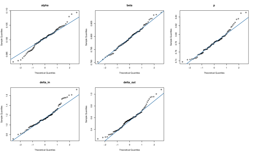
Figure 2. Q-Q plots for the estimates based on $100$ independently simulated HRNs with $\alpha=0.1$, $\beta=0.8$, $p=0.8$, $\delta_{\rm in}=1.3$ and $\delta_{\rm out}=0.7$.

Albeit the relatively better performance of the N-M method, the algorithm, as mentioned, undergoes the limitation of sensitivity to the initial value. Under the current setting, the N-M algorithm is able to provide estimation results over 90% of the simulation runs with a fixed initial start given by $\alpha^{(0)}=\beta^{(0)}=\gamma^{(0)}=1/3$, $p^{(0)}=1/2$ and $\delta_{\rm in}^{(0)}=\delta_{\rm out}^{(0)}=1$. When we use a random initial start (e.g., spacing $\alpha$, $\beta$ and $\gamma$ randomly on the unit interval, sampling $p$ from a standard uniform distribution and sampling $\delta_{\rm in}$ and $\delta_{\rm out}$ independently from a standard exponential distribution), the success rate may drop significantly to $60\%$ or less. The failure of the algorithm is primarily due to the inaccurate start of $\delta_{\rm in}$ and $\delta_{\rm out}$. We have also run some experiments on smaller networks. When reducing the simulated network size to 5,000, the success rate of the N-M algorithm declines to 35% or less even with a fixed initial simplex.

In contrast, the M-H algorithm is more robust, as it is always able to produce estimation results regardless of the size of the network. Specifically, we consider a random spacing of $\alpha$, $\beta$ and $\gamma$ on the unit interval, sample $\delta_{\rm in}$ and $\delta_{\rm out}$ independently from a standard exponential distribution, and let $p$ start from a value close to $1$ (e.g., $1-10^{-4}$), which indicates an almost perfect linear PA. Simulation results show that the choice of a non-informative prior of $p$ (i.e., sampling it uniformly from $[0,1]$) has negligible impact on the final estimation results. Though we observe bias in the estimates of $\delta_{\rm in}$ and $\delta_{\rm out}$, the 100% success rate renders the M-H method a competitive alternative.

To summarize, we recommend the N-M algorithm for parameter estimation if there is auxiliary information available to decide reasonable initial values. In addition, the M-H algorithm is a possible backup when the N-M algorithm fails. In practice, we may consider an integration of the two algorithms. Although the estimates of $\delta_{\rm in}$ and $\delta_{\rm out}$ from the M-H algorithm may not be very accurate, they are close enough to true values allowing for a successful implementation of the N-M algorithm. Therefore, we may first adopt the M-H algorithm to get coarse estimates of the model parameters, and use them as initial values for the N-M algorithm, which ultimately leads to finer estimation results. It is worth mentioning that this initial value selection procedure does not actually affect the estimation results by the N-M algorithm, but effectively increases the probability of the successful implementation of the N-M algorithm. If the target parameter is $p$ only but not $\delta_{\rm in}$ or $\delta_{\rm out}$, the estimation results from the M-H algorithm may have been acceptable.

6. Real Data Analysis

In this section, we fit the proposed HRN model to two real network datasets: the Dutch Wikipedia talk network and the Facebook wall posts, both of which are retrieved from the KONECT network data repository (http://konect.cc/). By investigating the timestamp information from both datasets, we see the existence of two additional edge creation scenarios at each step:

1. Set $J_{n}=4$ (with probability $0<\xi<1$) if a new node with a self-loop is added to the network;

2. Set $J_{n}=5$ (with probability $0<\eta<1$) if two new nodes with a directed edge connecting them are added to the network.

Note that these two additional scenarios require minor modifications of the log-likelihood given in Section 4, but they do not impose direct effect on the score functions of $p$, $\delta_{\rm in}$ and $\delta_{\rm out}$. The MLEs of $\xi$ and $\eta$ are straightforward:

$$\hat{\xi}^{\,\rm MLE}=\frac{1}{n}\sum_{k=1}^{n}\mathbb{I}_{\{J_{k}=4\}}\qquad\text{and}\qquad\hat{\eta}^{\,\rm MLE}=\frac{1}{n}\sum_{k=1}^{n}\mathbb{I}_{\{J_{k}=5\}}.$$

6.1. Dutch Wikipedia Talk

In the Dutch Wikipedia talk dataset, each single node represents a specific user of the Dutch Wikipedia, and the creation of a directed edge from node $u$ to node $v$ refers to the event that user $u$ leaves a message on user $v$’s talk page. The dataset includes the communication among the users of Dutch Wikipedia talk pages from 10/18/2002 and 11/23/2015, consisting of three columns. The first two columns represent users’ ID and the third column gives a UNIX timestamp with the time of a message posted on one’s Wikipedia talk page. For each row, the first user writes a message on the talk page of the second user at a timestamp given in the third column.

We select the sub-network according to the timestamp information from 01/01/2013 to 03/31/2013. The sub-network is directed, consisting of 3,288 nodes and 21,724 directed edges. We fit the proposed hybrid model to the data by using the integration of the M-H algorithm and the N-M algorithm. For the M-H algorithm, the burn-in number and iteration sample size are both set at 100,000, and the gap for thinning sampling is 500. The convergence of the estimates is checked via the time-series plots in Figure 3.

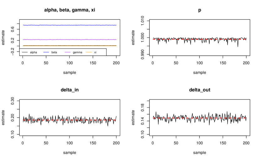
Figure 3. Graphical diagnostics of the convergence for the M-H algorithm applied to the sub-network of Dutch Wikipedia talk dataset; ; red dashed lines represent the estimated values.

Using the estimates from the M-H algorithm as the initial values for the N-M algorithm, we get almost identical estimates given by

$$\widehat{\bm{\theta}}_{\rm WK}:=(\hat{\alpha},\hat{\beta},\hat{\gamma},\hat{\xi},\hat{p},\hat{\delta}_{\rm in},\hat{\delta}_{\rm out})=(0.014,0.745,0.227,0.006,0.999,0.186,0.149),$$

where the value of $\hat{p}$ is extremely close to $1$. The large $\hat{p}$ suggests PA dominates the evolutionary process, thus leading to little difference between the proposed HRN and that proposed in Wan et al. [31]. For comparison, we compute the MLEs from the pure PA network model to get

$$\widehat{\bm{\theta}}_{\rm WK}^{\,\rm(PA)}:=(\hat{\alpha},\hat{\beta},\hat{\gamma},\hat{\xi},\hat{\delta}_{\rm in},\hat{\delta}_{\rm out})=(0.012,0.784,0.189,0.006,0.156,0.152),$$

from which we see the estimates from the two models are close to each other.

Figure 4. Out-degree and in-degree tail distributions of HRNs (red), directed PA networks (blue) and the sub-network of Dutch Wikipedia talk dataset (black).

Next, we simulate an HRN and a pure PA network with the estimated parameters, and plot their corresponding empirical tail distributions of the out- and in-degrees in Figure 4. As expected, the empirical out-degree and in-degree tail distributions from the two simulated networks are alike. It seems that the out-degree tail distribution (of the simulated networks) fits the real data better than the in-degree tail distribution, but the discrepancy between the in-degree tail distributions is also small.

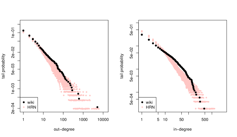
Figure 5. Out-degree and in-degree tail distributions of 50 independent HRNs (red), compared with those from the Wikipedia data (black).

In addition, we generate $50$ independent replications of the HRN using the given estimates. The out-degree and in-degree tail distributions of these simulated networks are collected in Figure 5. The left panel shows that the out-degree tail distribution of the selected sub-network is well covered by the overlaid plot of the simulated counterparts, whereas the right reveals small but acceptable discrepancy between the overlaid plot and the in-degree distribution of the real data. Overall, our analysis suggests the evolution of the selected sub-network of the Dutch Wikipedia talk data follows a linear PA mechanism, which also confirms the flexibility of the proposed hybrid model.

6.2. Facebook Wall Posts

The Facebook wall post dataset collects data from a regional network of users in New Orleans from 09/13/2004 to 01/21/2009. The data forms a directed graph where the nodes are Facebook users and each directed edge represents a post from one node to another node’s page. Like the previous one, this dataset contains three columns, where the first two contain the identifiers of the individual users, while the third records the timestamp of the corresponding post.

We select the sub-network based on the timestamp from 01/01/2006 to 06/31/2006, which consists of 4,200 nodes and 11,422 directed edges. Fitting the proposed hybrid model to the data, we get

$$\widehat{\bm{\theta}}_{\rm FB}:=(\hat{\alpha},\hat{\beta},\hat{\gamma},\hat{\xi},\hat{p},\hat{\delta}_{\rm in},\hat{\delta}_{\rm out})=(0.071,0.714,0.114,0.077,0.830,0.172,0.007).$$

The estimates are obtained via the integration of the N-M and M-H algorithms, where the settings of burn-in number, iteration size and thinning gap are identical to the previous example. In Figure 6, we verify the convergence of the estimates based on the M-H algorithm. Once again, we do not observe significant difference between the corresponding estimates from the two algorithms.

Figure 6. Graphical diagnostics of the convergence for the M-H algorithm applied to the sub-network of Facebook wall posts dataset; red dashed lines represent the estimated values.

We assess the goodness-of-fit of the model through the tail distributions of in-degree and out-degree. Specifically, we generate an HRN using $\widehat{\bm{\theta}}_{\rm FB}$, and compare the empirical out- and in-degree tail distributions from the simulated network with those from the real data. Results are presented in Figure 7. For comparison, we also fit a pure PA model to the same sub-network data using the estimation method derived in Wan et al. [31], and plot the corresponding empirical tail distributions (blue dots) in Figure 7.

Figure 7. Out-degree and in-degree tail distributions of HRNs (red), directed PA networks (blue) and the sub-network of Facebook wall posts (black).

The empirical tail distributions show that the HRN provides a better fit to the network data by introducing the extra UA rules controlled by the paramter $p$. Empirical out- and in-degree distributions from the pure PA model display heavier tails than those from the Facebook dataset, leading to a clear deviation from the data. In the HRN, however, the existence of $100(1-p)\%$ edges created by the UA rule has reduced the heaviness of the empirical tails, thus reducing the discrepancy between the empirical distributions.

Furthermore, we generate $50$ independent HRNs by using $\widehat{\bm{\theta}}_{\rm FB}$, and overlay their empirical out-degree and in-degree distributions in Figure 8. The graphical results show that the out-degree tail distribution is better captured by the HRN than the in-degree distribution, as it appears on the lower bound of the overlaid tail distributions of the simulated networks. The in-degree tail distribution of the Facebook sub-network is not covered by the counterparts of the simulated networks, though the shapes look similar and the deviation is not large.

Figure 8. Out-degree and in-degree tail distributions of 50 independent HRNs (red), compared with those from the Facebook data (black).

The discrepancy in Figure 8 may be due to the reciprocity feature in the Facebook wall posts. The wall posts activities among the Facebook users in a specific region tend to be reciprocated: when a friend posts a message on one’s wall, he/she is likely to reply quickly. In fact, using the reciprocity() function in the igraph package [7], we see that the proportion of reciprocated edges in the sub-network is over $0.18$. Indeed, the reciprocated wall posts are certainly not uniform, thus not very well characterized by the parameter $p$. To better study the reciprocity feature, we may consider other variants of the PA model, which are left as future work.

7. Discussion

In this paper, we propose a class of hybrid model simultaneously presenting the preferential attachment (PA) and uniform attachment (UA) mechanisms, which are governed by a tuning parameter $p$. Two standard methods, the Nelder-Mead (N-M) algorithm and the Metropolis-Hastings (M-H) algorithm, are adopted for parameter estimation. Through extensive simulations and a sensitivity study, we find that the N-M algorithm is preferred, but the corresponding success rate of producing estimation result depends heavily on the selection of the initial simplex. We thus consider an integrated approach where we use the more robust M-H algorithm to get the initial values for the target parameters, followed by the implementation of the N-M algorithm.

In addition, we fit the HRN model to two real network datasets: the Dutch Wikipedia talk and Facebook wall posts, where we see that the proposed hybrid model provides a more flexible modeling framework compared with the directed PA network model as in [31]. The extra tuning parameter $p$ helps correct the tail distributions of out- and in-degrees.

From the Facebook example, it is worth noting that even though the heaviness of the tail distributions (for both out- and in-degrees) has been weakened by $p$ in the HRN, the proposed UA part is not able to fully capture the reciprocity property in the real network. We here provide three classes of possible remedies: (1) It may be worthwhile to try some algorithmic approaches, such as network rewiring, to wash off the nodes of large in-degree or out-degree in the simulated networks; (2) We may consider modifying the model directly by introducing another parameter measuring the rate of reciprocation; (3) We may consider a more realistic mixer (some suitable light-tailed distribution) rather than simple UA in the present hybrid setting. We will report our research outcomes elsewhere in the future.

Appendix A Proof of Theorem 1

We explicitly demonstrate the derivations of the focusing theorem for the in-degree distribution, and the methodology is also applicable to out-degrees. Let $\mathcal{F}_{n}$ denote the $\sigma$-field generated by the network evolution up to $n$ steps. Set $\tau$ to be an $(\mathcal{F}_{n})_{n\geq 0}$-stopping time, then

$$\mathcal{F}_{\tau}=\{F:F\cap\{\tau=n\}\in\mathcal{F}_{n}\}.$$

For $i\geq 1$, let $S_{i}$ be the time when node $i$ is created, i.e.,

$$S_{i}=\inf\{n\geq 0:|V_{n}|=i\}.$$

Then $S_{i}$ is an $(\mathcal{F}_{n})_{n\geq 0}$-stopping time. Also, for $n\geq k\geq 0$, we have

$$\{S_{i}+k=n\}=\{S_{i}=n-k\}\in\mathcal{F}_{n-k}\subset\mathcal{F}_{n},$$

so $S_{i}+k$, $k\geq 0$, is a stopping time with respect to $(\mathcal{F}_{n})_{n\geq 0}$.

Since the in-degree of $i$ is increased at most by $1$ at each evolutionary step, the probability of the event $\{D^{\rm in}_{i}(S_{i}+n+1)=D^{\rm in}_{i}(S_{i}+n)\}$ under $\mathbb{P}^{\mathcal{F}_{S_{i}+n}}(\cdot):=\mathbb{P}(\cdot|\mathcal{F}_{S_{i}+n})$ is

$$\mathbb{P}^{\mathcal{F}_{S_{i}+n}} \left(D^{\rm in}_{i}(S_{i}+n+1)=D^{\rm in}_{i}(S_{i}+n)\right)$$

$$=1-(\alpha+\beta)\left[\frac{p(D^{\rm in}_{i}(S_{i}+n)+\delta_{\rm in})}{\sum_{k\in V_{S_{i}+n}}(D^{\rm in}_{k}(S_{i}+n)+\delta_{\rm in})}+\frac{(1-p)}{|V_{S_{i}+n}|}\right].$$

Therefore,

$$\mathbb{E}^{\mathcal{F}_{S_{i}+n}}\left[D^{\rm in}_{i}(S_{i}+n+1)\right]$$

$${}=D^{\rm in}_{i}(S_{i}+n)+(\alpha+\beta)\left[\frac{p(D^{\rm in}_{i}(S_{i}+n)+\delta_{\rm in})}{\sum_{k\in V_{S_{i}+n}}(D^{\rm in}_{k}(S_{i}+n)+\delta_{\rm in})}+\frac{(1-p)}{|V_{S_{i}+n}|}\right]$$

$$=D^{\rm in}_{i}(S_{i}+n)+(\alpha+\beta)\left[\frac{p(D^{\rm in}_{i}(S_{i}+n)+\delta_{\rm in})}{S_{i}+n+1+\delta_{\rm in}|V_{S_{i}+n}|}+\frac{(1-p)}{|V_{S_{i}+n}|}\right].$$ (15)

Write $C_{1}:=p(\alpha+\beta)/(1+\delta_{\rm in}(1-\beta))$, and $\tilde{\delta}_{\rm in}:=\delta_{\rm in}/p+(1-p)/(p(1-\beta))$, then we have

$$\mathbb{E}\left[D^{\rm in}_{i}(S_{i}+n+1)+\tilde{\delta}_{\rm in}\right]$$

$$\quad{}=\mathbb{E}\left[D^{\rm in}_{i}(S_{i}+n)+\tilde{\delta}_{\rm in}+(\alpha+\beta)\left(\frac{p(D^{\rm in}_{i}(S_{i}+n)+\delta_{\rm in})}{S_{i}+n+1+\delta_{\rm in}|V_{S_{i}+n}|}+\frac{(1-p)}{|V_{S_{i}+n}|}\right)\right]$$

$$\quad{}=\mathbb{E}\left[D^{\rm in}_{i}(S_{i}+n)+\tilde{\delta}_{\rm in}+(\alpha+\beta)\left(\frac{p(D^{\rm in}_{i}(S_{i}+n)+\tilde{\delta}_{\rm in})}{S_{i}+n+1+\delta_{\rm in}|V_{S_{i}+n}|}+\frac{(1-p)}{|V_{S_{i}+n}|}\right.\right.$$

$$\qquad\qquad{}-\left.\left.\frac{p(\tilde{\delta}_{\rm in}-\delta_{\rm in})}{S_{i}+n+1+\delta_{\rm in}|V_{S_{i}+n}|}\right)\right]$$

$$\quad{}=\mathbb{E}\left[(D^{\rm in}_{i}(S_{i}+n)+\tilde{\delta}_{\rm in})\left(1+\frac{p(\alpha+\beta)}{S_{i}+n+1+\delta_{\rm in}|V_{S_{i}+n}|}\right)\right]$$

$$\qquad{}\qquad{}+\mathbb{E}\left[\frac{1-p}{|V_{S_{i}+n}|}-\frac{p(\tilde{\delta}_{\rm in}-\delta_{\rm in})}{S_{i}+n+1+\delta_{\rm in}|V_{S_{i}+n}|}\right]$$

$$\quad{}\leq\mathbb{E}\left[(D^{\rm in}_{i}(S_{i}+n)+\tilde{\delta}_{\rm in})\left(1+\frac{p(\alpha+\beta)}{n+1+\delta_{\rm in}|V_{n}|}\right)\right]$$

$$\qquad\qquad{}+\frac{1-p}{n(1-\beta)}\mathbb{E}\left|(1-\beta)\frac{S_{i}+n+1}{|V_{S_{i}+n}|}-1\right|$$

$$\quad=\mathbb{E}\left[(D^{\rm in}_{i}(S_{i}+n)+\tilde{\delta}_{\rm in})\left(1+\frac{C_{1}}{n}\right)\right]$$

$$\qquad\qquad{}+\mathbb{E}\left[(D^{\rm in}_{i}(S_{i}+n)+\tilde{\delta}_{\rm in})\left(\frac{p(\alpha+\beta)}{n+1+\delta_{\rm in}|V_{n}|}-\frac{C_{1}}{n}\right)\right]$$

$$\qquad\qquad\qquad{}+\frac{1-p}{n(1-\beta)}\mathbb{E}\left|(1-\beta)\frac{S_{i}+n+1}{|V_{S_{i}+n}|}-1\right|$$

$$\quad=:I_{i}(n)+II_{i}(n)+III_{i}(n).$$ (16)

For $II_{i}(n)$, we have

$$II_{i}(n) \leq\mathbb{E}\left[(D^{\rm in}_{i}(S_{i}+n)+\tilde{\delta}_{\rm in})\left|\frac{p(\alpha+\beta)}{n+1+\delta_{\rm in}|V_{n}|}-\frac{C_{1}}{n}\right|\right]$$

$$\leq\mathbb{E}\left[(D^{\rm in}_{i}(S_{i}+n)+\tilde{\delta}_{\rm in})\frac{\delta_{\rm in}\bigl{|}|V_{n}|-(1-\beta)n\bigr{|}+1}{(1+\delta_{\rm in}(1-\beta))n^{2}}\right].$$

Since for $n\geq 1$, $|V_{n}|-1$ is a binomial random variable with success probability $1-\beta$, we apply the Chernoff bound to get

$$\mathbb{P}\left(\left||V_{n}|-(1-\beta)n\right|\geq\sqrt{12(1-\beta)n\log{n}}\right)\leq\frac{2}{n^{4}},$$ (17)

and noticing that $\left||V_{n}|-(1-\beta)n\right|\leq n$, and $D^{\rm in}_{i}(S_{i}+n)\leq n+1$, we have

$$II_{i}(n) \leq\left(\frac{\delta_{\rm in}\sqrt{12n\log n}}{n^{2}}+\frac{1}{n^{2}}\right)\mathbb{E}(D^{\rm in}_{i}(S_{i}+n)+\tilde{\delta}_{\rm in})$$

$$\qquad+\frac{2(\delta_{\rm in}n+1)(n+1+\tilde{\delta}_{\rm in})}{n^{6}}$$

$$\leq\left(\frac{\delta_{\rm in}\sqrt{12n\log n}}{n^{2}}+\frac{1}{n^{2}}\right)\mathbb{E}(D^{\rm in}_{i}(S_{i}+n)+\tilde{\delta}_{\rm in})+\frac{2(1+\delta_{\rm in})(2+\tilde{\delta}_{\rm in})}{n^{4}}.$$

For $III_{i}(n)$, we apply the Cauchy-Schwartz inequality to obtain

$$III_{i}(n) \leq\frac{1-p}{n(1-\beta)}\left(\mathbb{E}\left[\left((1-\beta)(S_{i}+n+1)-|V_{S_{i}+n}|\right)^{2}\right]\right)^{1/2}\left(\mathbb{E}\left[|V_{n}|^{-2}\right]\right)^{1/2}.$$

By Theorem 3.9.4 in [3], we have as $n\to\infty$,

$$n^{2}\mathbb{E}\left[|V_{n}|^{-2}\right]\to(1-\beta)^{-2}.$$

Meanwhile,

$$\mathbb{E} \left[\left((1-\beta)(S_{i}+n+1)-|V_{S_{i}+n}|\right)^{2}\right]$$

$$=\text{Var}\left(|V_{S_{i}+n}|\right)+\text{Var}\left((1-\beta)(S_{i}+n+1)\right)$$

$$=\beta(1-\beta)\left(\mathbb{E}\left(S_{i}\right)+n\right)+2(1-\beta)^{2}\text{Var}(S_{i}).$$

Hence, there exists some constant $A_{i}>0$ such that

$$III_{i}(n)\leq A_{i}n^{-3/2}.$$

Then it follows from (16) that

$$\mathbb{E} \left[D^{\rm in}_{i}(S_{i}+n+1)+\tilde{\delta}_{\rm in}\right]$$

$$\leq\mathbb{E}\left[(D^{\rm in}_{i}(S_{i}+n)+\tilde{\delta}_{\rm in})\left(1+\frac{C_{1}}{n}+\frac{1+\delta_{\rm in}\sqrt{12n\log n}}{n^{2}}\right)\right]$$

$$\quad+2(1+\delta_{\rm in})(2+\tilde{\delta}_{\rm in})n^{-4}+A_{i}n^{-3/2}.$$

Iterating backwards for $n$ times gives

$$\mathbb{E}\bigl{[}D^{\rm in}_{i}(S_{i}+n+1)+\delta_{\rm in}\bigr{]}$$

$$\quad{}\leq\bigl{(}\delta_{\rm in}\alpha+(1+\delta_{\rm in})\gamma\bigr{)}\prod_{r=1}^{n}\left(1+\frac{C_{1}}{r}+\frac{1+\sqrt{12(1-\beta)r\log r}}{r^{2}}\right)$$

$$\qquad{}+\sum_{r=1}^{n}\frac{2(1+\delta_{\rm in})(2+\tilde{\delta}_{\rm in})}{r^{2}}\prod_{s=r+1}^{n}\left(1+\frac{C_{1}}{s}+\frac{1+\sqrt{12(1-\beta)s\log s}}{s^{2}}\right).$$

Note that

$$\prod_{s=r+1}^{n}\left(1+\frac{C_{1}}{s}+\frac{1+\sqrt{12(1-\beta)s\log s}}{(1+\delta_{\rm in}(1-\beta))s^{2}}\right)$$

$$\quad{}\leq\exp\left\{\sum_{s=r+1}^{n}\left(\frac{C_{1}}{s}+\frac{1+\sqrt{12(1-\beta)s\log s}}{(1+\delta_{\rm in}(1-\beta))s^{2}}\right)\right\}$$

$$\quad{}\leq(n/r)^{C_{1}}\exp\left\{\sum_{s=1}^{\infty}\frac{1+\sqrt{12(1-\beta)s\log s}}{(1+\delta_{\rm in}(1-\beta))s^{2}}\right\},$$

which gives

$$\sup_{i\geq 1}\frac{\mathbb{E}[D^{\rm in}_{i}(n)]}{n^{C_{1}}}\leq\sup_{i\geq 1}\frac{\mathbb{E}[D^{\rm in}_{i}(S_{i}+n)+\tilde{\delta}_{\rm in}]}{n^{C_{1}}}<\infty.$$

This completes the proof.

Appendix B Proof of Theorem 2

Like the proof of Theorem 1, we only present the details for the in-degree sequence. The derivations for out-degree sequence are similar, so omitted.

For $k,\ell\geq 0$, we have

$$\mathbb{E}\left[M^{\rm in}_{k+\ell}-M^{\rm in}_{k}\right] =\sum_{s=k+1}^{k+\ell}\mathbb{E}\left[M^{\rm in}_{s}-M^{\rm in}_{s-1}\right]$$

$$=\sum_{s=k+1}^{k+\ell}\mathbb{E}\left[\frac{(1-p)(\alpha+\beta)/|V_{S_{i}+s}|}{\prod_{\ell=1}^{s}\left(1+\frac{p(\alpha+\beta)}{S_{i}+\ell+1+\delta_{\rm in}|V_{S_{i}+\ell}|}\right)}\right]$$

$$\leq\sum_{s=k+1}^{k+\ell}\mathbb{E}\left[\prod_{\ell=1}^{s}\left(1+\frac{p(\alpha+\beta)}{(1+\delta_{\rm in})(S_{i}+\ell+1)}\right)\frac{(1-p)(\alpha+\beta)}{|V_{S_{i}+s}|}\right]$$

$$\leq\sum_{s=k+1}^{k+\ell}\prod_{\ell=1}^{s}\left(1+\frac{p(\alpha+\beta)}{(1+\delta_{\rm in})(\ell+1)}\right)\mathbb{E}\left[\frac{(1-p)(\alpha+\beta)}{|V_{s}|}\right],$$

where

$$\prod_{\ell=1}^{s}\left(1+\frac{p(\alpha+\beta)}{(1+\delta_{\rm in})(\ell+1)}\right)=\frac{\Gamma\left(s+2+\frac{p(\alpha+\beta)}{1+\delta_{\rm in}}\right)}{\Gamma(s+2)\Gamma\left(2+\frac{p(\alpha+\beta)}{1+\delta_{\rm in}}\right)}\sim s^{-(p(\alpha+\beta))/(1+\delta_{\rm in})},$$

for $s$ large. For the expectation in the summand, we have

$$\mathbb{E}\left[\frac{(1-p)(\alpha+\beta)}{|V(s)|}\right]=(1-p)(\alpha+\beta)\left(\frac{1}{(1-\beta)s}+\mathbb{E}\left[\frac{1}{|V(s)|}-\frac{1}{(1-\beta)s}\right]\right).$$

By the Chernoff bound in (17), we get

$$\mathbb{E}\left[\left|\frac{1}{|V(s)|}-\frac{1}{(1-\beta)s}\right|\right] =\mathbb{E}\left[\frac{\bigl{|}|V(s)|-(1-\beta)s\bigr{|}}{(1-\beta)s|V(s)|}\right]$$

$$\leq\frac{\sqrt{12(1-\beta)s\log s}}{(1-\beta)s|(1-\beta)s-\sqrt{12(1-\beta)s\log{s}}|}$$

$$\qquad{}+\frac{(2-\beta)s}{(1-\beta)s\sqrt{12(1-\beta)s\log s}}\times\frac{2}{s^{4}}.$$

Putting them together, we conclude that $\mathbb{E}\left|M^{\rm in}_{k+\ell}-M^{\rm in}_{k}\right|\to 0$ as $k\to\infty$, suggesting that $\left\{\mathbb{E}\left[M^{\rm in}_{n}\right]\right\}_{n\geq 1}$ is a cauchy sequence in $L_{1}$ space. Applying the martingale convergence theorem [10, Theorem 4.2.11] gives that there exists some finite random variable $L_{i}$ such that as $n\to\infty$,

$$M^{\rm in}_{n}\stackrel{{\scriptstyle a.s.}}{{\longrightarrow}}L_{i}.$$ (1)

Then it remains to show the almost sure convergence of

$$X_{n}:=\prod_{k=0}^{n-1}\left(1+\frac{(\alpha+\beta)p}{S_{i}+k+1+\delta_{\rm in}|V_{S_{i}+k}|}\right).$$

Consider $\log X_{n}$, and rewrite it as

$$\log X_{n}= \left[\sum_{k=0}^{n-1}\log\left(1+\frac{(\alpha+\beta)p}{S_{i}+k+1+\delta_{\rm in}|V_{S_{i}+k}|}\right)-\sum_{k=0}^{n-1}\frac{(\alpha+\beta)p}{S_{i}+k+1+\delta_{\rm in}|V_{S_{i}+k}|}\right]$$

$$+\left[\sum_{k=0}^{n-1}\frac{(\alpha+\beta)p}{S_{i}+k+1+\delta_{\rm in}|V_{S_{i}+k}|}-\sum_{k=1}^{n}\frac{C_{1}}{S_{i}+k+1}\right]$$

$$+\left[\sum_{k=1}^{n}\frac{C_{1}}{S_{i}+k}-C_{1}\log n\right]$$

$$+C_{1}\log n=:P_{1}(n)+P_{2}(n)+P_{3}(n)+C_{1}\log n.$$ (2)

For $P_{1}(n)$, we first note that $\log(1+x)-x\leq 0$ for all $x\geq 0$. Then $P_{1}(n+1)-P_{1}(n)\leq 0$, i.e. $P_{1}(n)$ is decreasing in $n$, and it suffices to show

$$P_{1}(\infty):=\sum_{k=0}^{\infty}\left(\log\left(1+\frac{(\alpha+\beta)p}{S_{i}+k+1+\delta_{\rm in}|V_{S_{i}+k}|}\right)-\frac{(\alpha+\beta)p}{S_{i}+k+1+\delta_{\rm in}|V_{S_{i}+k}|}\right)$$

is finite almost surely. Note also that $|\log(1+x)-x|\leq x^{2}/2$, for all $x\geq 0$, then

$$\mathbb{E} \left|\sum_{k=0}^{\infty}\left(\log\left(1+\frac{(\alpha+\beta)p}{S_{i}+k+1+\delta_{\rm in}|V_{S_{i}+k}|}\right)-\frac{(\alpha+\beta)p}{S_{i}+k+1+\delta_{\rm in}|V_{S_{i}+k}|}\right)\right|$$

$$\leq\sum_{k=0}^{\infty}\mathbb{E}\left|\log\left(1+\frac{(\alpha+\beta)p}{S_{i}+k+1+\delta_{\rm in}|V_{S_{i}+k}|}\right)-\frac{(\alpha+\beta)p}{S_{i}+k+1+\delta_{\rm in}|V_{S_{i}+k}|}\right|$$

$$\leq\frac{(\alpha+\beta)^{2}p^{2}}{2}\sum_{k=0}^{\infty}\mathbb{E}\left(\frac{1}{S_{i}+k+1+\delta_{\rm in}|V_{S_{i}+k}|}\right)^{2}\leq\sum_{k=1}^{\infty}\frac{1}{k^{2}}<\infty.$$

Hence, $P_{1}(n)\,\overset{a.s.}{\longrightarrow}\,P_{1}(\infty)$.

For $P_{2}(n)$, we apply [3, Theorem 3.9.4] to conclude that there exists a finite r.v. $Z$ such that

$$\sum_{k=1}^{\infty}\left(\frac{(\alpha+\beta)p}{k+\delta_{\rm in}|V(k-1)|}-\frac{C_{1}}{k}\right)\,\overset{a.s.}{\longrightarrow}\,Z,$$

then

$$P_{2}(n)\,\overset{a.s.}{\longrightarrow}\,Z-\sum_{k=1}^{S_{i}}\left(\frac{(\alpha+\beta)p}{k+\delta_{\rm in}|V(k-1)|}-\frac{C_{1}}{k}\right)=:P_{2}(\infty).$$

Meanwhile, since $\sum_{k=1}^{n}1/k-\log n\to\tilde{c}$ as $n\to\infty$, where $\tilde{c}$ is Euler’s constant, then for $i\geq 1$,

$$P_{3}(n)\,\overset{a.s.}{\longrightarrow}\,C_{1}\left(\tilde{c}+\log(S_{i}+1)-\sum_{k=1}^{S_{i}}\frac{1}{k}\right)=:P_{3}(\infty).$$

Then we conclude from (2) that

$$\frac{X_{n}}{n^{C_{1}}}\,\overset{a.s.}{\longrightarrow}\,\exp\left(P_{1}(\infty)+P_{2}(\infty)+P_{3}(\infty)\right)<\infty.$$ (3)

The results in the theorem follow by combining (3) with (1), where we set

$$\zeta_{i}:=L_{i}\exp\left(-(P_{1}(\infty)+P_{2}(\infty)+P_{3}(\infty))\right).$$

Appendix C Proof of Theorem 3

Analogous to the previous proofs, we present the major steps of the proof for in-degree. Applying the argument as in the proof of [30, Proposition 8.4], we have the concentration result that

$$\frac{N^{\text{in}})_{m}(n)}{n}-\frac{\mathbb{E}\left(N^{\text{in}}_{m}(n)\right)}{n}\stackrel{{\scriptstyle p}}{{\longrightarrow}}0.$$

Then it suffices to find the asymptotic limit of $\mathbb{E}\left(N^{\text{in}}_{m}(n)\right)/{n}$.

We consider the approximation of the attachment probability:

$$\frac{p\bigl{(}D^{\rm in}_{i}(n)+\delta_{\rm in}\bigr{)}}{\bigl{(}1+\delta_{\rm in}(1-\beta)\bigr{)}n}+\frac{1-p}{(1-\beta)n}=\frac{D^{\rm in}_{i}(n)+\delta_{\rm in}+\frac{1-p}{p(1-\beta)}\bigl{(}1+\delta_{\rm in}(1-\beta)\bigr{)}}{\bigl{(}1+\delta_{\rm in}(1-\beta)\bigr{)}n/p}.$$

Recall that

$$\tilde{\delta}_{\rm in}=\delta_{\rm in}+\frac{1-p}{p(1-\beta)}\bigl{(}1+\delta_{\rm in}(1-\beta)\bigr{)}=\frac{\delta_{\rm in}}{p}+\frac{1-p}{p(1-\beta)}.$$

Using Chernoff bound in (1), we have

$$\left|\mathbb{E}\left[\frac{p\bigl{(}D^{\rm in}_{i}(n)+\delta_{\rm in}\bigr{)}}{n+1+|V_{n}|\delta_{\rm in}}+\frac{1-p}{|V_{n}|}\right]-\mathbb{E}\left[\frac{D^{\rm in}_{i}(n)+\tilde{\delta}_{\rm in}}{\bigl{(}1+\delta_{\rm in}(1-\beta)\bigr{)}n/p}\right]\right|$$

$$\quad{}\leq Cn^{-3/2}\sqrt{\log{n}},$$ (1)

for some constant $C>0$. Consider a in-degree sequence $\left\{\tilde{D}_{i}^{\rm in}(n)\right\}$ from a directed PA network with set of parameters $(\alpha,\beta,\gamma,\tilde{\delta}_{\rm in},\tilde{\delta}_{\rm out})$, as studied in  Samorodnitsky et al. [25], Wan et al. [31]. Establish an argument similar to Equation (17) as follows:

$$\left|\mathbb{E}\left[\frac{p\bigl{(}D^{\rm in}_{i}(n)+\delta_{\rm in}\bigr{)}}{n+1+|V_{n}|\delta_{\rm in}}+\frac{1-p}{|V_{n}|}\right]-\mathbb{E}\left[\frac{\tilde{D}_{i}^{\rm in}(n)-\tilde{\delta}_{\rm in}}{n+1+|V_{n}|\tilde{\delta}_{\rm in}}\right]\right|\leq\tilde{C}n^{-3/2}\sqrt{\log{n}},$$

for some constant $\tilde{C}>0$. Note

$$\mathbb{P}\bigl{(}D^{\rm in}_{i}(n)=m\bigr{)}=\sum_{j=m-1}^{m}\mathbb{P}\bigl{(}D^{\rm in}_{i}(n)=m\,|\,D^{\rm in}_{i}(n-1)=j\bigr{)}\mathbb{P}\bigl{(}D^{\rm in}_{i}(n-1)=j\bigr{)}.$$

By the developed Chernoff bounds, we have

$$\mathbb{P}\bigl{(}D^{\rm in}_{i}(n)=m\bigr{)}\leq\mathbb{P}\bigl{(}\tilde{D}_{i}^{\rm in}(n)=m\bigr{)}+(C+\tilde{C})\sum_{k=i}^{n}k^{-3/2}\sqrt{\log{k}}.$$

Noticing that $\sum_{k=i}^{n}k^{-3/2}\sqrt{\log{k}}<\infty$ as $n\to\infty$, we complete the proof by applying the results derived in Wang and Resnick [35].

References

• Alves et al. [2019] Alves, C., R. Ribeiro, and R. Sanchis (2019). Preferential attachment random graphs with edge-step functions. Journal of Theoretical Probability. DOI: https://doi.org/10.1007/s10959-019-00959-0.
• Atalay et al. [2011] Atalay, E., A. Hortaçsu, J. Roberts, and C. Syverson (2011). Network structure of production. Proceedings of the National Academy of Sciences of the United States of America 108(13), 5199–5202.
• Athreya and Ney [2004] Athreya, K. and P. Ney (2004). Branching processes. Reprint of the 1972 original. Springer.
• Barabási and Albert [1999] Barabási, A.-L. and R. Albert (1999). Emergence of scaling in random networks. Science 286(5439), 509–512.
• Chen et al. [2010] Chen, M.-H., Q.-M. Shao, and J. G. Ibrahim (2010). Monte Carlo Methods in Bayesian Computation. New York, NY, U.S.A.: Springer-Verlag.
• Clauset et al. [2009] Clauset, A., Shalizi, C., Newman, M. (2009) Power-law distributions in empirical data. SIAM Rev, 51(4):661–703.
• Csardi and Nepusz [2006] Csardi, G. and T. Nepusz (2006). The igraph software package for complex network research. InterJournal Complex Systems, 1695.
• Dereich and Mörters [2009] Dereich, S., Mörters, P. (2009) Random networks with sublinear preferential attachment: degree evolutions. Electronic Journal of Probability, 14:1222–1267.
• Drees et al. [2020] Drees, H., Janßen, A., Resnick, S.I., Wang, T. (2020) On a minimum distance procedure for threshold selection in tail analysis. SIAM Journal on Mathematics of Data Science, 2(1):75–102.
• Durrett [2006] Durrett, R. T. (2006). Random Graph Dynamics. Cambridge, U.K.: Cambridge University Press.
• Gao and van der Vaart [2017] Gao, F. and A. van der Vaart (2017). On the asymptotic normality of estimating the affine preferential attachment network models with random initial degrees. Stochastic Processes and their Applications 127(11), 3754–3775.
• Gelman et al. [2013] Gelman, A., J. B. Carlin, D. B. Dunson, A. Behtari, and D. B. Rubin (2013). Bayesian Data Analysis. Boca Raton, FL, U.S.A.: Chapman and Hall/CRC.
• Hasselman [2018] Hasselman, B. (2018). nleqslv: Solve systems of nonlinear equations. CPB Netherlands Bureau for Economic Policy Analysis. R package version 3.3.2, https://CRAN.R-project.org/package=nleqslv.
• Hastings [1970] Hastings, W. K. (1970). Monte Carlo sampling methods using Markov chains and their applications. Biometrika 57(1), 97–109.
• Henzinger and Lawrence [2004] Henzinger, M. and S. Lawrence (2004). Extracting knowledge from the World Wide Web. Proceedings of the National Academy of Sciences of the United States of America 101(supplement 1), 5186–5191.
• Lagarias et al. [1998] Lagarias, J. C., J. A. Reeds, M. H. Wright, and P. E. Wright (1998). Convergence properties of the Nelder-Mead simplex method in low dimensions. SIAM Journal on Optimization 9(1), 112–147.
• Liang et al. [2010] Liang, F., C. Liu, and R. J. Carroll (2010). Advanced Markov Chain Monte Carlo Methods: Learning from Past Examples. Hoboken, NJ, U.S.A.: John Wiley & Sons.
• Mahmoud [2019] Mahmoud, H. M. (2019). Local and global degree profiles of randomly grown self-similar hooking networks under uniform and preferential attachment. Advances in Applied Mathematics 111, 101930.
• Mengersen and Tweedie [1996] Mengersen, K. L. and R. L. Tweedie (1996). Rates of convergence of the Hastings and Metropolis algorithms. Annals of Statistics 24(1), 101–121.
• Merton [1968] Merton, R. K. (1968). The Matthew Effect in science. Science 159(3810), 56–63.
• Metropolis et al. [1953] Metropolis, N., A. W. Rosenbluth, N. Rosenbluth, Marshall, and A. H. Teller (1953). Equation of state calculations by fast computing machines. The Journal of Chemical Physics 21, 1087.
• Nelder and Mead [1965] Nelder, J. A. and R. Mead (1965). A simple method for function minimization. The Computer Journal 7(4), 308–313.
• Newman [2001] Newman, M. E. J. (2001). Clustering and preferential attachment in growing networks. Physical Review E 65(1), 025102.
• Pachon et al. [2018] Pachon, A., L. Sacerdote, and S. Yang (2018). Scale-free behavior of networks with the copresence of preferntial and uniform attachment rules. Physica D: Nonliner Phenomena 371, 1–12.
• Samorodnitsky et al. [2016] Samorodnitsky, G., S. Resnick, D. Towsley, R. Davis, A. Willis, and P. Wan (2016, March). Nonstandard regular variation of in-degree and out-degree in the preferential attachment model. Journal of Applied Probability 53(1), 146–161.
• Shao et al. [2006] Shao, Z.-G., X.-W. Zou, and Z.-Z. Jin (2006). Growing networks withmixed attachment mechanisms. Journal of Physics A: Mathematical and General 39, 9.
• Smith [2007] Smith, B. J. (2007). boa: An R package for MCMC output convergence assessment and posterior inference. Journal of Sstatistical Software 21(11), 1–37.
• Soetaert [2009] Soetaert, K. (2009). rootSolve: Nonlinear root finding, equilibrium and steady-state analysis of ordinary differential equations. Netherlands Institute of Ecology. R package 1.6, https://cran.r-project.org/web/packages/rootSolve/rootSolve.pdf.
• de Sollar Price [1965] de Sollar Price, D. J. (1965). Networks of scientific papers. Science 149(3683), 510–515.
• van der Hofstad [2017] van der Hofstad, R. (2017). Random Graphs and Complex Networks. Cambridge, U.K.: Cambridge University Press.
• Wan et al. [2017] Wan, P., T. Wang, R. A. Davis, and S. I. Resnick (2017). Fitting the linear preferential attachment model. Electronic Journal of Statistics 11(2), 3738–3780.
• Wang and Resnick [2018] Wang, T. and S. Resnick (2018). Multivariate regular variation of discrete mass functions with applications to preferential attachment networks. Methodology and Computing in Applied Probability 20(3), 1029–1042.
• Wang and Resnick [2020] Wang, T. and S. Resnick (2020). Degree growth rates and index estimation in a directed preferential attachment model. Stochastic Processes and their Applications 130(2), 878–906.
• Wang and Resnick [2015] Wang, T. and S. I. Resnick (2015). Asymptotic normality of in- and out-degree counts in a preferential attachment model. Stochastic Models 33(2), 229–255.
• Wang and Resnick [2020] Wang, T. and S. I. Resnick (2020). A directed preferential attachment model with Poisson measurement. https://arxiv.org/pdf/2008.07005.pdf.
• Zhang and Mahmoud [2020] Zhang, P. and H. M. Mahmoud (2020). On nodes of small degrees and degree profile in preferential dynamic attachment circuits. Methodology and Computing in Applied Probability 22(2), 625–645.