Adversary Instantiation: Lower Bounds for Differentially Private Machine Learning

Abstract

Differentially private (DP) machine learning allows us to train models on private data while limiting data leakage. DP formalizes this data leakage through a cryptographic game, where an adversary must predict if a model was trained on a dataset $D$, or a dataset $D^{\prime}$ that differs in just one example. If observing the training algorithm does not meaningfully increase the adversary’s odds of successfully guessing which dataset the model was trained on, then the algorithm is said to be differentially private. Hence, the purpose of privacy analysis is to upper bound the probability that any adversary could successfully guess which dataset the model was trained on.

In our paper, we instantiate this hypothetical adversary in order to establish lower bounds on the probability that this distinguishing game can be won. We use this adversary to evaluate the importance of the adversary capabilities allowed in the privacy analysis of DP training algorithms.

For DP-SGD, the most common method for training neural networks with differential privacy, our lower bounds are tight and match the theoretical upper bound. This implies that in order to prove better upper bounds, it will be necessary to make use of additional assumptions. Fortunately, we find that our attacks are significantly weaker when additional (realistic) restrictions are put in place on the adversary’s capabilities. Thus, in the practical setting common to many real-world deployments, there is a gap between our lower bounds and the upper bounds provided by the analysis: differential privacy is conservative and adversaries may not be able to leak as much information as suggested by the theoretical bound.

I Introduction

With machine learning now being used to train models on sensitive user data, ranging from medical images [19], to personal email [8] and text messages [53], it is becoming ever more important that these models are privacy preserving. This privacy is both desirable for users, and increasingly often also legally mandated in frameworks such as the GDPR [11].

Differential privacy (DP) is now the standard definition for privacy [14, 15]. While first defined as a property a query mechanism satisfies on a database, differential privacy analysis has since been extended to algorithms for training machine learning models on private training data  [7, 4, 51, 1, 38, 55, 25, 47, 20, 21]. On neural networks, differentially private stochastic gradient descent (DP-SGD) [1, 4, 51] is the most popular method to train neural networks with DP guarantees. Differential privacy sets up a game where the adversary is trying to guess whether a training algorithm took as its input one dataset $D$ or a second dataset $D^{\prime}$ that differs in only one example. If observing the training algorithm’s outputs allows the adversary to improve their odds of guessing correctly, then the algorithm leaks private information. Differential privacy proposes to randomize the algorithm in such a way that it becomes possible to analytically upper bound the probability of an adversary making a successful guess, hence quantifying the maximum leakage of private information.

In recent work [26] proposed to audit the privacy guarantees of DP-SGD by instantiating a relatively weak, black-box adversary who observed the model’s predictions. In this paper, we instantiate this adversary with a spectrum of attacks that spans from a black-box adversary (that is only able to observe the model’s predictions) to a worst-case yet often unrealistic adversary (with the ability to poison training gradients and observe intermediate model updates during training). This not only enables us to provide a stronger lower bounds on the privacy leakage (compared to [26]), it also helps us identify which capabilities are needed for adversaries to be able to extract exactly as much private information as is possible given the upper bound provided by the DP analysis.

Indeed, in order to provide strong, composable guarantees that avoid the pitfalls of other privacy analysis methods [35, 36, 52], DP and DP-SGD assume the existence of powerful adversaries that may not be practically realizable.

Figure 1: Summary of our results, plotting emperically measured $\varepsilon$ when training a model with $\varepsilon=2$ differential privacy on MNIST. The dashed red line corresponds to the certifiable upper bound. Each bar correspond to the privacy offered by increasingly powerful adversaries. In the most realistic setting, training with privacy offers much more empirically measured privacy. When we provide full attack capabilities, our lower bound shows that the DP-SGD upper bound is tight.

For example, the DP-SGD analysis assumes that the intermediate computations used to train a model are published to the adversary, when in most practical settings only the final, fully-trained model is revealed. This is done not because it is desirable—but because there are limited (known) ways to improve the analysis by assuming the adversary has access to only one model [21]. As such, it is conceivable—and indeed likely—that the actual privacy in practical scenarios is greater than what can be shown theoretically (indeed, DP-SGD is known to be tight asymptotically [4]).

Researchers have often assumed that this will be true [27], and argue that it is acceptable to train models with guarantees so weak that they are essentially vacuous, hoping that the actual privacy offered is much stronger [6]. This is important because training models with weak guarantees generally allows one to achieve greater model utility, which often leads practitioners to follow this train of thought when tuning their DP training algorithms.

I-A Our Techniques

We build on the poisoning adversary introduced in Jagielski et al. [26]. By adversarially constructing two datasets $D$ and $D^{\prime}$ we can audit DP-SGD. Concretely, we instantiate the hypothetical differential privacy adversary under various adversary scenarios by providing a pair of concrete attack algorithms: one that constructs the two datasets $D$ and $D^{\prime}$ differing in one example, and another that receives a model as input (that was trained on one of these two datasets) and predicts which one it was trained on.

We use these two adversaries as a tool to measure the relative importance of the assumptions made by the DP-SGD analysis, as well as the potential benefits of assumptions that are not currently made, but could be reasonable assumptions to make in the future. Different combinations of assumptions correspond to different threat models and constraints on the adversary’s capabilities, as exposed in Sections IV-A to IV-F.

There are two communities who this analysis impacts.

• Practitioners would like to know the privacy leakage in situations that are as close to realistic as possible. Even if it is not possible to prove tight upper bounds of privacy, we can provide best-effort empirical evidence that the privacy offered by DP-SGD is greater than what is proven when the adversary is more constrained.

• Theoreticians, conversely, care about identifying ways to improve the current analysis. By studying various capabilities that a real-world adversary would actually have, but that the analysis of DP-SGD does not assume are placed on the adversary, we are able to estimate the potential utility of introducing additional assumptions.

I-B Our Results

Figure 1 summarizes our key results. When our adversary is given full capabilities, our lower bound matches the provable upper bound, demonstrating the DP-SGD analysis is tight in the worst-case. In the past, more sophisticated analysis techniques (without making new assumptions) were able to establish better and better upper bounds on essentially the same DP-SGD algorithm [1]. This meant that we could train a model once, and over time its privacy would “improve” (so to speak), as progress in theoretical work on differential privacy yielded a tighter analysis of the same algorithm used to train the model. Our lower bound implies that this trend has come to an end, and new assumptions will be necessary to establish tighter bounds.

Conversely, the bound may be loose under realistic settings, such as when we assume a more restricted adversary that is only allowed to view the final trained model (and not every intermediate model obtained during training). In this setting, our bound is substantially lowered and as a result it is possible that better analysis might be able to improve the privacy bound.

Finally, we show that many of the capabilities allowed by the adversary do not significantly strengthen the attack. For example, the DP-SGD analysis assumes the adversary is given access to all intermediate models generated throughout training; surprisingly, we find that access to just the final model is almost as good as all prior models.

On the whole, our results have broad implications for those deploying differentially private machine learning in practice (for example, indicating situations where the empirical privacy is likely stronger than the worst case) and also implications for those theoretically analyzing properties of DP-SGD (for example, indicating that new assumptions will be required to obtain stronger privacy guarantees).

II Background & Related Work

II-A Machine Learning

A machine learning model is a parameterized function $f_{\theta}\colon\mathcal{X}\to\mathcal{Y}$ that takes inputs from an input space $\mathcal{X}$ and returns outputs from an output space $\mathcal{Y}$. The majority of this paper focuses on the class of functions $f_{\theta}$ known as deep neural networks [34], represented as a sequence of linear layers with non-linear activation functions [43]. Our results are independent of any details of the neural network’s architecture.

The model parameters $\theta$ are obtained through a training algorithm $\mathcal{T}$ that minimize the average loss $\ell(f_{\theta},x,y)$ on a finite-sized training datasets $D=\{(x_{i},y_{i})\}_{i=1}^{|D|}$, denoted by $\mathcal{L}(f_{\theta},D)$. Formally, we write $f_{\theta}\leftarrow\mathcal{T}(D).$

Stochastic gradient descent [34] is the canonical method for minimizing this loss. We sample a mini-batch of examples

$$\mathbb{B}(D)=B=\{(x_{i},y_{i})\}_{i=1}^{|B|}\subset D.$$

Then, we compute the average mini-batch loss as

$$\mathcal{L}(f_{\theta};B)={1\over|B|}\sum_{(x,y)\in B}\ell(f_{\theta};x,y)$$

and update the model parameters according to

$$\theta_{i+1}\leftarrow\theta_{i}-\eta\nabla_{\theta}\mathcal{L}(f_{\theta_{i}};B)$$ (1)

taking a step of size $\eta$, the learning rate. We abbreviate each step of this update rule as $f_{\theta+1}\leftarrow\mathcal{S}(f_{\theta},B)$.

Because neural networks are trained on a finite-sized training dataset, models train for multiple epochs repeating the same examples over and over, often tens to hundreds of times. This has consequences for the privacy of the training data. Machine learning models are often significantly over-parameterized [50, 56]: they contain sufficient capacity to memorize the particular aspects of the data they are trained on, even if these aspects are irrelevant to final accuracy. This allows a wide range of attacks that leak information about the training data given access to the trained model. These attacks range from membership inference attacks [6, 24, 39, 45, 50, 49] to training data extraction attacks [22, 39].

II-B Differential Privacy

Differential privacy (DP) [14, 16, 17] has become the de-facto definition of algorithmic privacy. An algorithm $\mathcal{M}$ is said to be $(\varepsilon,\delta)$-differentially private if for all set of events $S\subseteq\text{Range}(\mathcal{M})$, for all neighboring data sets $D,D^{\prime}\in\mathcal{D}^{n}$ (where $\mathcal{D}$ is the set of all possible data points ) that differ in only one sample:

$$\Pr[\mathcal{M}(D)\in S]\leq e^{\varepsilon}\Pr[\mathcal{M}(D^{\prime})\in S]+\delta.$$

Informally, this definition requires the probability any adversary can observe a difference between the algorithm operating on dataset $D$ versus a neighboring dataset $D^{\prime}$ is bounded by $e^{\varepsilon}$, plus a constant additive failure rate of $\delta$. To provide a meaningful theoretical guarantee, $\varepsilon$ is typically set to small single digit numbers, and $\delta\ll 1/|D|$. Other variants of DP use slightly different formulations (e.g., Rényi differential privacy [40] and concentrated DP [18, 5]); our paper studies predominantly this $(\varepsilon,\delta)$-definition of DP as it is the most common. Furthermore, it is often possible to translate a property achieved under one formulation to another, in fact the DP-SGD analysis uses a Rényi bound as an intermediate step to achieving the $(\varepsilon,\delta)$ bounds.

Differential privacy has two useful properties we will use. First, the composition of multiple differentially private algorithms is still differentially private (adding their respective privacy budgets). Second, differential privacy is immune to post-processing: the output of any DP algorithm can be arbitrarily post-processed while retaining the same privacy guarantees.

Consider the toy problem of reporting the approximate sum of $D=\{x_{1},\dots,x_{n}\}$ with each $x_{i}\in[-1,1]$. A standard way to compute a DP sum is the Gaussian mechanism [17]:

$$\mathcal{M}(D)=\sum_{x_{i}\in D}x_{i}+Z\hskip 14.22636pt\text{where }Z\sim\mathcal{N}(0,\sigma^{2})$$ (2)

If $\sigma=\sqrt{2\log(1.25/\delta)}/\varepsilon$, then it can be shown that $\mathcal{M}$ guarantees $(\epsilon,\delta)$-differential privacy—because each sample has a bounded range of $1$. If $x_{i}$ was unbounded, for any fixed amount of noise $\sigma$, it would always be possible to let

$$\hat{D}=\left\{2\sigma,0,\dots,0\right\},\hskip 14.22636pt\tilde{D}=\left\{-2\sigma,0,\dots,0\right\}$$

so with high probability $\mathcal{M}(D)>0$ if and only if $D=\hat{D}$.

II-C Differentially-Private Stochastic Gradient Descent

Stochastic gradient descent (SGD) can be made differentially private through two straightforward modifications. Proceed initially as in SGD, and sample a minibatch of examples randomly from the training dataset. Then, as in Equation 1, compute the gradient of the loss on this mini-batch with respect to the model parameters $\theta$. However, before directly applying this gradient $\nabla_{\theta}\mathcal{L}(f_{\theta},B)$ DP-SGD first makes the gradient differentially private. Intuitively, we achieve this by (1) bounding the contribution of any individual training example, and then (2) adding a small amount of noise. Indeed, this can be seen as an application of the Gaussian mechanism to the gradients updates.

To begin, DP-SGD clips the gradients so that any individual update is bounded in magnitude by $b$, and then adds Gaussian noise whose scale $\sigma$ is proportional to $b$. After sampling a minibatch $B=\mathbb{B}(\mathcal{X})$, the new update rule becomes

$$\theta_{i+1}\leftarrow\theta_{i}-\eta\left({1\over|B|}\sum_{(x,y)\in B}\text{clip}_{b}\left(\nabla_{\theta}\ell(f_{\theta_{i}},x,y)\right)+Z_{i}\right)$$ (3)

where $Z_{i}\sim\mathcal{N}(0,\sigma^{2}\mathbb{I})$ and $\text{clip}_{b}(v)$ is the function that projects $v$ onto the $\ell_{2}$ ball of radius $b$ with

$$\text{clip}_{b}(v)=v\cdot\min\left\{1,\frac{b}{\|v\|_{2}}\right\}.$$

It is not difficult to see how one would achieve $(\varepsilon,\delta)$-DP guarantees following Equation 2. To achieve $(\varepsilon,\delta)$-DP, typically $\sigma$ is in the order of $\Omega(q\frac{\sqrt{T\log(\frac{1}{\delta})}}{\varepsilon})$ [1]. Moreover, Mironov et. al. [41] showed tighter bounds for a given $\sigma$. On each iteration, we are computing a differentially-private update of the model parameters given the gradient update $\nabla_{\theta}\ell$ through the subsampled Gaussian Mechanism. Then, because DP is immune to post-processing, we can apply these gradients to the model. Finally, through composition, we can obtain a guarantee for the entire model training pipeline.

However, it turns out that naive composition using this trivial analysis gives values of $\varepsilon\gg 10^{4}$ for accurate neural networks, implying a ratio of adversary true positive to false positive bounded by $e^{10^{4}}$—and hence not meaningful. Thus, Abadi et al. [1] develop the Moments Accountant: an improvement of Bassily et al. [4] which introduces a much more sophisticated tool to analyze DP-SGD that can prove, for the same algorithm, values of $\varepsilon<10$. Since then, many works [13, 2, 54, 41, 31, 3] improved the analysis of the Moments Accountant analysis to get better theoretical privacy bounds.

This raises our question: is the current analysis the best analysis tool we could hope for? Or does there exist a stronger analysis approach that could, again for the same algorithm—but perhaps with different (stronger) assumptions—reduce $\varepsilon$ by orders of magnitude?

III Analysis Approach: Adversary Instantiation

We answer this question and analyze the tightness of the DP-SGD analysis under various assumptions by instantiating the adversary against the differentially private training algorithm. This gives us a lower bounds on the privacy leakage that may result. Our primary goal is to not only investigate the tightness of DP-SGD under any one particular set of assumptions [26], but also to understand the relative importance of adversary capabilities assumed to establish this upper bound. This allows us to appreciate what practical conditions need to be met before an adversary exploits the full extent of the privacy leakage tolerated by the upper bound. This section develops our core algorithm: adversary instantiation. We begin with our motivations to construct this adversary (§ III-A) present the algorithm (§ III-B) and then describe how to use this algorithm to lower bound privacy (§ III-C).

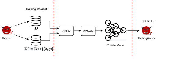
Figure 2: Our attack process. Our first algorithm, the crafter constructs two datasets $D$ and $D^{\prime}$ differing in one example. The model trainer then (independently of the adversary) trains a model on one of these two datasets. Our second algorithm, the distinguisher then guesses which dataset was used.

III-A Motivation: Adversary Capabilities

The analysis of DP-SGD is an over-approximation of actual adversaries that occur in practice. This is for two reasons. First, there are various assumptions that DP-SGD requires that are necessarily imposed because DP captures more powerful adversaries than typically exist. Second, there are adversary restrictions that we would immediately choose to enforce if there was a way to do so, but currently have no way to make use of in the privacy analysis. We briefly discuss each of these.

Restrictions imposed by DP

Early definitions of privacy were often dataset-dependent definitions. For example, $k$-anonymity argues (informally) that a data sample is private if there are at least $k$ “similar” [52]. Unfortunately, these privacy definitions often have problems when dealing with high dimensional data [44]—allowing attacks that nevertheless reveal sensitive information.

In order to avoid these difficulties, differential privacy makes dataset-agnostic guarantees: $(\varepsilon,\delta)$-DP must hold for all datasets $D$, even for pathologically constructed datasets $D$. It is therefore conceivable that the total privacy afforded to any user in a “typical” dataset might be higher than if they were placed in the worst-case dataset for that user.

Restrictions imposed by the analysis

The second class of capabilities are those allowed by the proof that the DP-SGD update rule (Equation 3) satisfies differential privacy, but if it were possible to improve the analysis by preventing these attacks it would be done. Unfortunately, there is no known way to improve on the analysis by prohibiting these particular capabilities—even if we believe that it should help.

The canonical example of this is the publication of intermediate models. The DP-SGD analysis assumes the adversary is given all intermediate model updates $\{\theta_{i}\}_{i=1}^{N}$ used to train the neural network, and not just the final model. These assumptions is not made because it is necessary to satisfying differential privacy, but because the only way we know how to analyze DP-SGD is through a composition over mini-batch iterations, where the adversary learned all intermediate updates.

In the special case of training convex models, it turns out there is a way to directly analyze the privacy of the final learned model [21]. This gives a substantially stronger guarantee than can be proven by summing up the cumulative privacy loss over each iteration of the training algorithm. However, for general deep neural networks, there are no known techniques to achieve this. Hence, we ask the question: does having access to the intermediate model updates allow an adversary to mount an attack that leaks more private information from a deep neural network’s training set?

Similarly, the analysis in differential privacy assumes the adversary has direct control of the gradient updates to the model. Again however, this is often not true in practice: the inputs to a machine learning training pipeline are input examples, not gradients. The gradients are derived from the current model and the worst-case inputs. The proofs place the the trust boundary at the gradients simply because it is simpler to analyze the system this way. If it was possible to analyze the algorithm at the more realistic interface of examples, it would be done. Through our work, we are able to show when doing so would not improve the upper bound, in which case it would be unnecessary to attempt an improvement of the analysis that relaxes this assumption.

III-B Instantiating the DP Adversary

Because assumptions made to analyze the privacy of DP-SGD appear conservative, researchers often conjecture that the privacy afforded by DP-SGD is significantly stronger than what can be proven. For example, Carlini et al. [6] argue (and provide some evidence) that training language models with $\varepsilon=10^{5}$-DP might be safe in practice despite this offering no theoretical guarantees. In other words, it is assumed that there is a gap between the lower bound an adversary may achieve when attacking the training algorithm and the upper bound established through the analysis.

Before we expend more effort as a community to improve on the DP-SGD analysis to tighten the upper bound, it is important to investigate how wide it may be. If we could show that the gap is non-existent, there would be no point in trying to tighten the analysis, and instead, we would need to identify additional constraints that could be placed on the adversary in order to decrease the worst-case privacy leakage. This motivates our alternate method to measure privacy with a lower bound, through developing an attack. This lets us directly measure how much privacy restricting each of these currently-allowed capabilities would afford, should we be able to analyze the resulting training algorithm strictly.

As the core technical contribution of this paper, in order to measure this potential gap left by the privacy analysis of DP-SGD, we instantiate the adversary introduced in the formulation of differential privacy. The objective of the theoretical DP adversary is to distinguish between a model $f$ that was either trained on dataset ${D}$ or on dataset ${D}^{\prime}$, where the datasets only differ at exactly one instance. Thus, our instantiated adversary consists of two algorithms: the first algorithm chooses the datasets ${D}$ and ${D^{\prime}}$, after which a model is trained on one of these at random, and then the second algorithm predicts which dataset was selected and trained on. Figure 2 gives a schematic of our attack approach containing the three phases of our attack, described in detail below.

The Crafter

The Crafter adversary is a randomized algorithm taking no inputs and returning two possible sets of inputs to model training algorithm $\mathcal{T}$. Intuitively, this adversary corresponds to the differential privacy analysis being data-independent: it should hold for all pairs of datasets which only differ by one point. We will propose concrete implementations later in Section IV-A through IV-F. Formally, we denote this adversary by the function $\mathcal{A}$. In most cases, this means that $\mathcal{A}\to({D},(x^{*},y^{*}))$, with ${D^{\prime}}={D}\cup\{(x^{*},y^{*})\}$.

Model training (not adversarial).

After the Crafter has supplied the two datasets, the training algorithm runs in a black box outside of the control of the adversary. The model trainer first randomly chooses one of the two datasets supplied by the adversary, and then trains the model on this dataset (either for one step or the full training run). Depending on the exact details of the training algorithm, differing levels of information are revealed to the adversary. For example, the standard training algorithm in DP-SGD is assumed to reveal all intermediate models $\{\theta_{i}\}_{i=1}^{N}$. We denote training by the randomized algorithm $t=\mathcal{T}({D})$.

The Distinguisher

The Distinguisher adversary is a randomized algorithm $\mathcal{B}\to\{0,1\}$ that predicts $0$ if $\mathcal{T}$ was trained on ${D}$ (as produced by $\mathcal{A}$), and $1$ if ${D}^{\prime}$. This corresponds to the differential privacy analysis which estimates how much an adversary can improve its odds of guessing whether the training algorithm learned from $D$ or $D^{\prime}$.

The Distinguisher receives as input two pieces of data: the output of Crafter, and the output of the model training process. Thus, in all cases the Distinguisher receives the two datasets produced by Crafter, however in some setups when the Crafter is called multiple times, the Distinguisher receives the output of all runs. Along with this, the Crafter receives the output of the training process, which again depends on the experimental setup. In most cases, this is either the final trained model weights $\theta_{N}$ or the sequence of weights $\{\theta_{i}\}_{i=1}^{N}$.

III-C Lower Bounding $\varepsilon$

Performing a single run of the above protocol gives a single bit: either the adversary wins (by correctly guessing which dataset was used during training) or not (by guessing incorrectly). In order to be able to provide meaningful analysis, we must repeat the above attack multiple times and compute statistics on the resulting set of trials.

We follow an analysis approach previously employed to audit DP [12, 26]. We extend the analysis to be able to reason about both pure DP where $\delta=0$ and the more commonly employed $(\varepsilon,\delta)$ variant, unlike prior work which assumes $\delta$ is always negligible [26]. We define one instance of the attack as the Crafter choosing a pair of datasets, the model being trained on one of these, and the Distinguisher making its guess. For a fixed training algorithm we would like to run, we define a pair of adversaries. Then, we run a large number of instances on this problem setup. Through Monte Carlo methods, we can then compute a lower bound on the $(\varepsilon,\delta)$-DP.

Given the success or failure bit from each instance of the attack, we compute the false positive and false negative rates. Defining the positive and negative classes is arbitrary; without loss of generality we define a a false positive as the adversary guessing ${D}^{\prime}$ when the model was trained on ${D}$, and vice versa for a false negative. Kairouz et. al [29] showed if a mechanism $\mathcal{M}$ is $(\epsilon,\delta)$-differentially private then the adversary’s false positive (FP) and false negative (FN) rate is bounded by:

$$FP+e^{\varepsilon}FN\leq 1-\delta\hskip 30.00005ptFN+e^{\varepsilon}FP\leq 1-\delta$$

Therefore, given an appropriate $\delta$, we can determine the empirical $(\varepsilon,\delta)-$differential privacy as

$$\varepsilon_{empirical}=\max(\log\frac{1-\delta-FP}{FN},\log\frac{1-\delta-FN}{FP})$$ (4)

Using the Clopper-Pearson method [10], we can determine confidence bounds on the attack performance. This lets us determine a lower confidence bound on the empirical $\varepsilon$ as

$$\varepsilon_{empirical}^{lower}=\max(\log\frac{1-\delta-FP^{high}}{FN^{high}},\log\frac{1-\delta-FN^{high}}{FP^{high}})$$ (5)

where $\mathit{FP}^{high}$ is the high confidence bound for false positive and $\mathit{FN}^{high}$ is the high confidence bound for false negative.

We repeat most of our experiments 1000 times in order to measure the FPR and FNR. Even if the adversary were to succeed in all 1000 of the trials, the Clopper-Pearson bound would imply an epsilon lower bound of 5.60. Note that as a result of this, it will never be possible for us to establish a lower bound greater than $\varepsilon=5.60$ with 1000 trials and a confidence bound of due solely to statistical power.

Section	Experiment	Access	Modification	Dataset	Protocol	Adversaries		Results
§ IV-A	API access	Black-box	Random Sample	Not modified	Protocol 1	Crafter 1	Distinguisher 1	Fig. 3
§ IV-B	Static Poison Input	Final Model	Malicious Sample	Not modified	Protocol 1	Crafter 2	Distinguisher 1	Fig. 4
§ IV-C	Intermediate Attack	Intermediate Models	Malicious Sample	Not modified	Protocol 2	Crafter 2	Distinguisher 2	Fig. 5
§ IV-D	Adaptive Poison Input	Intermediate Models	Adaptive Sample	Not modified	Protocol 3	Crafter 3	Distinguisher 2	Fig. 6
§ IV-E	Gradient Attack	Intermediate Models	Malicious Gradient	Not modified	Protocol 4	Crafter 4	Distinguisher 3	Fig. 7
§ IV-F	Dataset Attack	Intermediate Models	Malicious Gradient	Malicious	Protocol 4	Crafter 5	Distinguisher 3	Fig. 8

TABLE I: Experiment settings. We run attacks under six set of adversary capabilities; each experiment increases the capabilities of the adversary ranging from the weakest membership inference adversary to the strongest adversary with full DP capabilities.

IV Experiments

Having developed the methodology to establish a lower bound on differential privacy guarantees, we now apply it across six attack models, where we vary adversary capabilities around four orthogonal key aspects of the ML pipeline.

• Access. What level of access does the adversary have to the output of the training algorithm?

• Modification. How does the adversary perform the manipulations of the training dataset?

• Dataset. Does the adversary control the entire dataset? Or just one poisoned example? Or is the dataset assumed to be a typical dataset (e.g., CIFAR10)?

While it would (in principle) be possible to evaluate the effect of every possible combination of the assumptions, it is computationally intractable. Thus, we describe six possible useful configurations, where by useful we mean configurations which correspond to relevant modern deployments of ML (e.g., MLaaS, federated learning, etc.) or key aspects of the privacy analysis. Table I summarizes the adversaries we consider. Note that some of the attacks use similar Crafter or Distinguisher, we did not repeat the identical algorithms. Please refer to Table I for the Crafter or Distinguisher for each attack. Below we describe them briefly and relate them to one another before expanding on them in the remainder of this section. Note that we do not argue that any particular set of assumptions can provide a specific privacy bounds, but rather that it cannot be more private than our experimental bounds.

API access: The data owner will collect the data and train the model itself, the adversary cannot control and modify the training procedure or dataset. The adversary can only have black box access to the trained model. This setting is the most practical attack: it is a running example in the ML security literature given the increased popularity of the ML as a Service (MLaaS) deployment scenario. In this most realistic yet limited evaluation, we establish a baseline lower bound through a membership inference attack [49].

Static Poison Attack: While “typical-case” privacy leakage is an important factor in understanding privacy risk, it is also worth evaluating the privacy of worst-case outliers. For example, when training a model on a dataset containing exclusively individuals of one type (age, gender, race, etc), it is important to understand if inserting a training example from an under-represented group would increase the likelihood of private information leaking from the model. To study this setting, we instantiate our adversary to construct worst-case malicious inputs, and has access to the final trained model.

Intermediate Poison Attack: As mentioned earlier, the DP-SGD analysis assumes the adversary is given access to all intermediate model parameters. We repeat the above attack, but this time reveal all intermediate models. This allows us to study the relative importance of this additional capability.

Adaptive Poison Attack: The DP-SGD analysis does not have a concept of a dataset: it operates solely on gradients computed over minibatches of training data. Thus, there is no requirement that the one inserted example remains the same between epochs: at each iteration, we re-instantiate the worst-case inserted example after each epoch. This again allows us to evaluate whether the minibatch perspective taken in the analysis affects the lower bound we are able to provide.

Gradient Attack: As federated learning continues to receive more attention, it is also important to estimate how much additional privacy leakage results from training a model in this environment. In federated learning a malicious entity can poison the gradients themselves. As mentioned in Section II-C, DP-SGD also assumes the adversary has access to the gradients, therefore we mount an attack where the adversary modifies the gradient directly.

Dataset Attack: In our final and most powerful attack, we make use of all adversary capabilities. The DP-SGD analysis yields a guarantee which holds for all pairs of datasets with a Hamming distance of 1, even if these datasets are pathological worst-case datasets. Thus, in this setting, we allow the adversary to construct such a pathalogical dataset. Evaluating this setting is what allows us to demonstrate that the DP-SGD analysis is tight. The tightness of the DP-SGD privay bounds in the worst case can also be inferred from the theoretical analysis [13, 41], however, the main purpose of this evaluation is to show that our attack can be tight when the adversary is the most powerful. If we could not reach the provable upper bound, then we would have no hope that our results would be tight in the other settings. Moreover, we crafted a specific attack to achieve the highest possible privacy leakage.

IV-A API Access Adversary

As a first example of how our adaptive analysis approach proceeds, we consider the baseline adversary who mounts the well-researched membership inference attack [49] in a setting where they have access to an API. As described above, this corresponds to the most practical setting—a black-box attack where the attacker is only given access to an API revealing the model’s output (its confidence so has to be able to compute the loss) on inputs chosen by the attacker. The schematic for this analysis is given in Protocol 1.

Membership Inference Adversary Game
Adversary		Model Trainer
$(D,D^{\prime})\stackrel{{\scriptstyle\mathclap{\scriptsize\mbox{\$}}}}{{\leftarrow}}\mathcal{A}$		$b\stackrel{{\scriptstyle\mathclap{\scriptsize\mbox{\$}}}}{{\leftarrow}}\{0,1\}$
		$f_{\theta}\leftarrow\mathcal{T}(B_{b})$
$s\leftarrow\mathcal{B}(f_{\theta},D,x^{*},y^{*})$
		Check if $s=b$

List of Protocols 1 Adversary game for membership inference attack. Round 1. The adversary chooses two datasets. Round 2. The model trainer randomly trains a model on one of these, and returns the model. Round 3. The adversary predicts which dataset was used for training.

Crafter

(Crafter 1) Given any standard machine learning dataset ${D}$, we can remove a random example from the dataset to construct a new dataset ${D}^{\prime}$ that differs from ${D}$ in exactly one record. Formally, let $(x,y)\stackrel{{\scriptstyle\mathclap{\scriptsize\mbox{\$}}}}{{\leftarrow}}\mathcal{D}$ be a sample from the underlying data distribution at random. We let $\mathcal{A}=\{D,D\cup\{(x,y)\}\}$, We formalize this in Crafter 1.

Crafter 1 Membership Inference Adversary

0:  existing training dataset ${D}$, underlying data distribution $\mathcal{D}$

1:  $(x,y)\stackrel{{\scriptstyle\mathclap{\scriptsize\mbox{\$}}}}{{\leftarrow}}\mathcal{D}$

2:  ${D}^{\prime}\leftarrow{D}\cup\{(x,y)\}$

3:  return  ${D},{D}^{\prime}$

Model training

Recall from Section Appendix A: Experimental Setup that the trainer gets two datasets: $D$ and $D^{\prime}$. Then the trainer selects one of these datasets randomly and trains a model on the selected dataset using pre-defined hyperparameters. After training completes, the trainer outputs the trained model $f_{\theta}$.

Distinguisher

(Distinguisher 1) After the model $f_{\theta}$ has been trained, the Distinguisher now guesses which dataset was used by computing the loss of the trained model on the one differing example $\ell(f_{\theta},x,y)$. It guesses that the model was trained on ${D}^{\prime}$ if the loss is sufficiently small, and guess that it was trained on ${D}$ otherwise. In the rest of the paper, we refer to the differing example $(x,y)$ as the query input. Details are given in Distinguisher 1.

Distinguisher 1 Membership Inference Adversary

0:  model $f_{\theta}$, query input $(x,y)$, threshold $\tau$

1:  $L\leftarrow\ell(f_{\theta},x,y)$

2:  if  $L\leq\tau$ then

3:     return  $D^{\prime}$

4:  end if

5:  return  $D$

Previous works [48, 45, 39, 9] showed that if an instance is part of the training dataset of the target model, its loss is most likely less than the case when it is not part of the training dataset. That is, in this attack, we provide our instantiated adversary with an extremely limited power. In particular, the attacker has much less capabilities than what is assumed to analyze the differential privacy guarantees provided by DP-SGD. Protocol 1 summarizes the attack.

Results

Typically, membership inference is studied as an attack in order to learn if a given user is a member of the training dataset or not. However, we do not study it as an attack, but as a way to provide a lower bound on the privacy leakage that arises from training with DP-SGD.

We experiment with a neural network using three datasets commonly used in privacy research: MNIST [33], CIFAR-10 [32], and Purchase. The first two of these are standard image classification datasets, and Purchase is the shopping records of several thousand online customers, extracted during Kaggle’s “acquire valued shopper” challenge [28]. Full details of these datasets is given in Appendix VI-A

In each trial, we follow Protocol 1 for each of the three datasets. We train a differentially private model using DP-SGD setting $\varepsilon$ to typical values used in the machine learning literature: 1, 2, 4, and 10. As mentioned before, the more trials we perform the better we are able to establish a lower bound of $\varepsilon$. Due to computational constraints, we are limited to performing the attack $1,000$ times. These experiments took 3,000 GPU hours, parallelized over 24 GPUs.

When we perform this attack on the CIFAR-10 dataset and train a model with $\varepsilon=4$ differential privacy, the attack true positive rate is $0.017$ and false positive is $0.002$. By using the Clopper-Pearson method, we can probabilistically lower-bound this attack performance; for example, when we have performed $1000$ trials, there is a $95\%$ probability that the attack false positive rate is lower than $0.01$. Using Equations 4 and 5, we can convert empirical lower bound of $(\varepsilon,\delta)$-DP with $(0.31,10^{-5})$. This value is substantially lower than the provably correct upper bound of $(4,10^{-5})$.

Figure 3: Membership inference attack: the adversary only adds one sample from the underlying data distribution.

Figure 3 shows the empirical epsilon for the other datasets and values of differential privacy. For the MNIST dataset, the adversary’s advantage is not significantly better than random chance; we hypothesize that this is because MNIST images are all highly similar, and so inserting or removing any one training example from the dataset does not change the model by much. CIFAR-10 and Purchase, however, are much more diverse tasks and the adversary can distinguish between two dataset ${D}$ and ${D}^{\prime}$ much more easily. In general, the API access attack does not utilize any of the assumptions assumed to be available to the adversary in the DP-SGD analysis and as a consequence the average input from the underlying data distribution does not leak as much private information as suggested by the theoretical upper bound. However, as the tasks get more complex information leakage increases.

There are two possible interpretations of this result, which will be the main focus of this paper:

1. Interpretation 1. The differentially private upper bound is overly pessimistic. The privacy offered by DP-SGD is much stronger than the bound which can be proven.

2. Inteerpretation 2. This attack is weak. A stronger attack could have succeeded more often, and as such the bounds offered by DP-SGD might be accurate.

Prior work has often observed this phenomenon, and for example trained models with $\varepsilon=10^{5}$-DP [6] despite this offering almost no theoretical privacy, because empirically the privacy appeared to be strong. However, as we have already revealed in the introduction, it turns out that Interpretation 2 is correct: while, for this weak attack, the bounds are loose, this does not imply DP-SGD itself is loose when an adversary utilizes all capabilities.

IV-B Static Input Poisoning Adversary

The previous attack assumes a weak adversary to establish the first baseline lower bound in a realistic attack setting. Nothing constructed by $\mathcal{A}$ is adversarial per se, but rather selected at random from a pre-existing dataset. This subsection begins to strengthen the adversary.

Differential privacy bounds the leakage when two datasets ${D}$ and ${D}^{\prime}$ differ in any instance. Thus, by following prior work [26], we create an adversary that crafts a poisoned malicious input $x$ such that when the model trains on this input, its output will be different from the case where the instance is not included—thus making membership inference easier.

The Crafter

(Crafter 2) Inspired by Jagielski et al. [26], we construct an input designed to poison the ML model. Given access to samples from the underlying data distribution, the adversary trains a set of shadow models (e.g., as done in [49]). The adversary trains shadow models using the same hyperparameters as the model trainer will use, which allows adversary to approximate how model trainer’s model will behave. Next, the adversary generates an input with an adversarial example algorithm [42]. If a model trains on that input, the learned model be different from a model which is not trained on that input. Crafter 2 summarizes the algorithm.

Crafter 2 Static Adversary Crafting

0:  train dataset ${D}_{shadow}$, adversarial train steps $T$, input learning rate $s$, model learning rate $lr$, training dataset ${D}$

1:  $f^{shadow}_{1},\cdots,f^{shadow}_{n}\leftarrow\mathcal{T}_{dpsgd}({D}_{shadow})$

2:  $x,y\stackrel{{\scriptstyle\mathclap{\scriptsize\mbox{\$}}}}{{\leftarrow}}$ random sample from ${D}_{shadow}$

3:  for  $T$ times do

4:     $l_{malicious}\leftarrow\frac{1}{n}\sum_{i=1}^{n}\ell(f^{shadow}_{i},x,y)$

5:     $x\leftarrow x+s\nabla_{x}l_{malicious}$

6:  end for

7:  ${D}^{\prime}={D}\cup\{(x,y)\}$

8:  return  ${D},{D}^{\prime}$

Model training

Identical to prior.

The Distinguisher

(Distinguisher 1) Identical to prior.

Figure 4: Malicious input attack: the adversary has blackbox access. The maliciously crafted input leaks more information than a random sample from the data distribution.

Results

As visualized in Figure 4, this adversary is able to leverage its poisoning capability to leak more private information and achieve a higher empirical lower bound compared to the previous attack. This is consistent across all datasets. This is explained by the fact that the poisoned input is a worst-case input for membership inference whereas previously the attack was conducted on average-case inputs drawn from the training distribution. The results suggest that DP-SGD bounds are bounded below by a factor of $10\times$.

IV-C Intermediate Poison Attack

The DP-SGD privacy analysis assumes the existence of an adversary who has complete access to the model training pipeline, this includes intermediate gradients computed to update the model parameter values throughout training. Instead of the final model only, we now assume the Distinguisher is given access to these intermediate model parameters values, as shown in Protocol 2. (In the case of convex models, it is known that releasing all intermediate models gives the adversary no more power than just the final model, however there is no comparable theory for the case of deep neural networks.)

Intermediate Model Adversary Game
Adversary		Model Trainer
$(D,D^{\prime})\stackrel{{\scriptstyle\mathclap{\scriptsize\mbox{\$}}}}{{\leftarrow}}\mathcal{A}$
		$b\stackrel{{\scriptstyle\mathclap{\scriptsize\mbox{\$}}}}{{\leftarrow}}\{0,1\}$
		$\{f_{\theta_{i}}\}_{i=1}^{N}\leftarrow\mathcal{T}(B_{b})$
$s\leftarrow\mathcal{B}(\{f_{\theta_{i}}\},D,D^{\prime})$
		Check if $s=b$

List of Protocols 2 Adversary game for intermediate model adversary. Round 1. The adversary chooses two datasets. Round 2. The model trainer randomly trains a model on one of these, and returns the full sequence of model updates. Round 3. The adversary predicts which dataset was used for training.

Crafter

(Crafter 2) Identical to prior.

Model training

The model trainer gets the two datasets ${D}$ and ${D}^{\prime}$ from the Crafter. As before we train on one of these two datasets. However, this time, the trainer reveals all intermediate models from the stochastic gradient descent process $\{f_{\theta_{i}}\}_{i=1}^{N}$ to the Distinguisher.

Distinguisher

(Distinguisher 2) Given the sequence of trained model parameters, we now construct our second adversary to guess which dataset was selected by the trainer. We modify Crafter 1 to leverage access to the intermediate outputs of training. Instead of only looking at the final model’s loss on the poisoned instance, our adversary also analyzes intermediate losses. We compute either the average or maximum loss for the poisoned examples over all of the intermediate steps and guess the model was trained on $D$ if the loss is smaller than a threshold. We took the best attacker between the maximum and average variants. In our experiments, for smaller epsilons ($\varepsilon\leq 2$) the maximum worked better. For epsilons larger than $2$, it was instead the average. Distinguisher 2 outlines the resulting attack.

Distinguisher 2 White-box Membership attack

0:  all intermediate steps to step $T$ $f_{1},\cdots,f_{T}$, query input $(x,y)$, threshold $\tau$, attack method (max or mean)

1:  if attack method is max then

2:     $L\leftarrow\max_{i=1}^{T}\ell(f_{\theta_{i}},x,y)$

3:  end if

4:  if attack method is mean then

5:     $L\leftarrow\frac{1}{T}\sum_{i=1}^{T}\ell(f_{\theta_{i}},x,y)$

6:  end if

7:  if  $L<\tau$ then

8:     return  $D^{\prime}$

9:  end if

10:  return  $D$

Results

Our results in Figure 5 show that this adversary only slightly outperforms our previous adversary with access to the final model parameters only. This suggests that access to the final model output by the training algorithm leaks almost as much information as the gradients applied during training. This matches what the theory for convex models suggests, even though deep neural networks are non-convex.

Figure 5: Malicious input attack: the adversary has white-box access to the training dataset. The results are slightly better compared to the malicious input with blackbox access.

IV-D Adaptive Poisoning Attack

Recall that the DP-SGD analysis treats each iteration of SGD independently, and uses (advanced) composition methods to compute the final privacy bounds. As a result, there is no requirement that the dataset processed at iteration $i$ need be the same as the dataset used at another iteration $j$.

We design new adversaries to take advantage of this additional capability. As in the previous attack, our goal is to design two datasets with the property that training on them yields different models. Again, we will use a query input to distinguish between the models, but for the first time we will not directly place the query input in the training data. Instead, we will insert a series of (different) poison inputs, each of which is designed to make the models behave differently on the query input. We describe this process in detail below.

Adaptive Input Poisoning Adversary Game
Adversary		Model Trainer
$(x,y)\stackrel{{\scriptstyle\mathclap{\scriptsize\mbox{\$}}}}{{\leftarrow}}\mathcal{A}_{query}$		$b\stackrel{{\scriptstyle\mathclap{\scriptsize\mbox{\$}}}}{{\leftarrow}}\{0,1\}$
$({D},D^{\prime})\stackrel{{\scriptstyle\mathclap{\scriptsize\mbox{\$}}}}{{\leftarrow}}\mathcal{A}(f_{\theta_{i}},x,y)$			}3*[ Repeat $N$ Iterations ]
	$\theta_{i+1}\leftarrow\mathcal{S}(\mathbb{B}(B_{b}^{i},x,y),\theta_{i})$
	⋮
$s\leftarrow\mathcal{B}(\{f_{\theta_{i}}\},{D},D^{\prime})$
		Check if $s=b$

List of Protocols 3 Adversary game for adaptive input poisoning attack. Round 0. The adversary generates a query input. Round 2i. The adversary chooses datasets $D$, $D^{\prime}$ given the current weights $\theta_{i}$. Round 2i+1. The model trainer trains for one minibatch on one of these datasets. Round N. The adversary predicts which dataset was used for training.

Crafter

(Crafter 3) We first generate a query input $(x_{q},y_{q})$ by calling Crafter 2 from the prior section: this is the input that the Distinguisher will use to make its guess. Then, on each iteration of gradient descent, we generate a fresh example $(x,y)$ such that if the model $f$ trains on ${D}\backslash\{(x,y)\}$, we expect that the loss of the query input $x_{q}$ will be significantly larger than training on the full ${D}$, i.e. $\ell(f^{{D}\backslash\{(x,y)\}},x_{q},y_{q})\ll\ell(f^{{D}},x_{q},y_{q}).$

To generate the malicious input $x$, we perform double backpropagation. We compute the gradient of the query input’s loss, given a model trained on $x$. Then, we temporarily apply this gradient update, and then again take a gradient this time updating $x$ so that it will minimize the loss of the query input. This process is described in Crafter 3.

Crafter 3 Dynamic Malicious Generation

0:  current model $f_{\theta_{T}}$, train steps $T$, input learning rate $s$, model learning rate $lr$

1:  $(D_{a},D^{\prime}_{a})\leftarrow$ Crafter 2

2:  $x_{query},y_{query}\leftarrow D^{\prime}_{a}\backslash D_{a}$

3:  $x,y\leftarrow$ $\vec{0}$

4:  for  $T$ times do

5:     $l_{model}\leftarrow\ell(f,x,,y)$

6:     $f^{\prime}(x)\leftarrow f(x)-lr\times\nabla_{f_{\theta_{T}}}l_{model}$

7:     $l_{malicious}\leftarrow\ell(f^{\prime},x_{query},y_{query})$

8:     $x\leftarrow x+s\nabla_{x}l_{malicious}$

9:  end for

10:  ${D}^{\prime}={D}\cup\{(x,y)\}$

11:  return  ${D},{D}^{\prime}$

Model training

As usual, the model trainer randomly chooses to train on the benign dataset $D$ or the malicious dataset $D^{\prime}$. If $D$ is selected, training proceeds normally. Otherwise, before each iteration of training, the trainer runs  Crafter 3 first to get an updated malicious $D^{\prime}$ and selects a mini-batch from the given dataset. Recall that here, we are interested in the attack for the purpose of establishing a lower bound so while this attack assumes strong control from the adversary on the dataset, it allows us to more accurately bound any potential privacy leakage.

Distinguisher

(Distinguisher 2) This adversary is unchanged from the prior section, as described in Distinguisher 2. However, as indicated above, we use the query input $(x_{query},y_{query})$ instead of the poison examples that are inserted into the training data.

Results

Figure 6 summarizes results for this setting. Compared to the previous attack, the adversary now obtains a tighter lower bound on privacy. For example, on the Purchase dataset with $\varepsilon=2$, this adaptive poisoning attack can achieve a lower-bound $\varepsilon_{lower}=0.37$ compared to $0.25$ in the prior section. Having the ability to modify the training dataset at each iteration was the missing key to effectively exploit access to the intermediate model updates and obtain tighter bounds.

Figure 6: Adaptive malicious input attack: the adversary changes the training dataset in each iteration. The adversary can achieve better results compared to prior attacks.

IV-E Gradient attack

By taking a closer look at the DP-SGD formulation, we see that the analysis assumes the adversary is allowed to control not only the input examples $x$, but the gradient updates $\nabla_{\theta}\ell(f_{\theta},x,y)$ themselves. The reason this is allowed is because the clipping and noising is applied at the level of gradient updates, regardless of how they were obtained. Thus, even though we intuitively know that the update vector was generated by taking the gradient of some function, the analysis does not make this assumption anywhere. While this assumption might not be true in every setting, in federated learning [37, 30, 48] the participants can directly modify the gradient vectors, which can be a possible setting to deploy such an attack. Nevertheless, we are interested in evaluating this adversary primarily to understand what additional power this gives the adversary.

All prior attacks relied on measuring the model’s loss on some input example to distinguish between the two datasets. Unlike the previous attacks, the Distinguisher this time will directly inspect the weights of the neural network.

Gradient Poisoning Adversary Game
Adversary		Model Trainer
		$b\stackrel{{\scriptstyle\mathclap{\scriptsize\mbox{\$}}}}{{\leftarrow}}\{0,1\}$
$\mathcal{G},\mathcal{G}^{\prime}\stackrel{{\scriptstyle\mathclap{\scriptsize\mbox{\$}}}}{{\leftarrow}}\mathcal{A}(f_{\theta_{i}})$			}4*[ Repeat $N$ Iterations ]
		$B\leftarrow\mathbb{B}(B_{b}^{i})$
$B_{dp}\leftarrow\{\text{clip}_{p}(x)+N\,\colon\,x\in B\}$
$\theta_{i+1}\leftarrow\theta_{i}-\eta\sum_{x\in B_{dp}}x$
	⋮
$s\leftarrow\mathcal{B}(\{f_{\theta_{i}}\},\mathcal{G})$
		Check if $s=b$

List of Protocols 4 Adversary game for gradient poisoning attack. Round 2i. The adversary chooses a collection of gradients $\mathcal{G},\mathcal{G}^{\prime}$. Round 2i+1. The model trainer chooses a subset of one of these gradient updates, and updates the parameters using the clipped and noised gradients. Round 2N. The adversary predicts which dataset was used for training.

The Crafter

(Crafter 4) The Crafter inserts a watermark into the model parameters. To minimize the effect of modifying these parameters, the adversary selects a set of model parameters which leave the model’s performance on training data largely unaffected. The Crafter modifies model parameters whose gradients are smallest in magnitude: intuitively, these model parameters are not updated much during training so they are good candidates for being modified. In particular for the first $t_{o}$ iterations of training, the adversary observes the model parameters’ gradient and after $t_{o}$ iterations, it selects $2n$ parameters which have the smallest sum of gradient absolute values. Crafter 4 outlines this procedure.

Crafter 4 Gradient attack

0:  intermediate models up to step $T$ $f^{1},\cdots,f^{t}$, clipping norm $C$, number of poison parameters $2n$, number of measurements $T_{o}$, training dataset $D$

1:  $M\leftarrow\sum_{t=1}^{\min(T_{o},T)-1}|f^{t+1}-f^{t}|$

2:  $points\leftarrow\text{select smallest 2n arguments from}M$

3:  $\nabla_{malicious}\leftarrow\vec{0}$

4:  $s\leftarrow 1$

5:  for $p$ in $points$ do

6:     $\nabla_{malicious}[p]=s\frac{C}{\sqrt{2n}}$

7:     $s=-s$

8:  end for

9:  

10:  $\mathcal{G}\leftarrow\{\}$

11:  for $(x,y)\in D$  do

12:     $\mathcal{G}.\text{insert}(\nabla l(f,x,y))$

13:  end for

14:  return  $\mathcal{G},\mathcal{G}\cup\nabla_{malicious}$

Model training

The model randomly selects to train on $D$ or $D^{\prime}$. If the trainer selects $D^{\prime}$, the trainer calls Crafter 4 to obtain a malicious gradient. It also selects a batch from the training dataset and computes the corresponding private gradient update, then with probability $q$ it adds the malicious gradient from Crafter 4. The model trainer reveals the model parameters for all of the intermediate steps to the attacker.

The Distinguisher

(Distinguisher 3) Given the collection of model weights $\{\theta_{i}\}_{i=1}^{N}$, the Distinguisher adversary will directly inspect the model weights to make its guess. Similar to the Crafter, the adversary observes the gradient of the first $t_{o}$ iterations to find which $2n$ model parameters has the smallest overall absolute value. Since the Crafter tries to increase the distance between these model parameters, to detect if such watermark exist in the model parameters, the Distinguisher computes the distance between the parameters, and then performs hypothesis testing to detect the presence of a watermark. The distance from the set of parameters either come from the gradient distribution ($Z$) plus the added Gaussian noise (i.e, null hypothesis), or are watermarked which means they come from the gradient distribution plus the added Gaussian noise plus the watermark:

$$H_{null}\,:\,\,Z+\mathcal{N}(0,\sigma^{2})\quad H_{watermark}\,:\,Z+\mathcal{N}(\frac{C}{\sqrt{2n}},\sigma^{2})$$

Since the Crafter chooses the parameters with smallest changes, we assume the gradient of these points are zero. This lets us simplify the problem to finding out if the distance between the parameters are coming from a Gaussian with mean zero or with mean equal to the sum of the distances between the watermarked parameters. Now, given the distance between the watermarked parameters, we can compute the likelihood of it coming from the watermarked gradient as:

$$p(Distance=d|watermark)=\frac{1}{2\sqrt{\pi n\sigma^{2}}}\exp{-(\frac{(x-C)^{2}}{2\sigma^{2}})}$$ (6)

where $2n$ is the number of selected parameters, $C$ and $\sigma$ are the clipping norm and the scale used to clip and noise gradients in DP-SGD, and $d$ is the distance computed by Distinguisher 3

Distinguisher 3 Watermark detection

0:  subsampling rate $q$, number of iterations $T$, clipping norm $C$, number of poison parameters $2n$,number of measurements $t_{o}$ , trained models $f_{0},\cdots f_{T}$, threshold $\tau$

1:  $M\leftarrow\vec{0}$

2:  $p_{watermark}\leftarrow 1$

3:  for $t=1$ to $T$ do

4:     if $t\leq t_{o}$ then

5:        $M=M+|f_{t}-f_{t-1}|$

6:     else

7:        $points\leftarrow\text{select smallest 2n arguments from}M$

8:        $\nabla_{malicious}\leftarrow\vec{0}$

9:        $s\leftarrow 1$

10:        $d\leftarrow 0$

11:        for $p$ in $points$ do

12:           $d=d+s\cdot f_{t}-f_{t-1}[p]$

13:           $s=-s$

14:        end for

15:        $p_{watermark}=p_{watermark}\times p(d|watermark)$

16:     end if

17:  end for

18:  if  $p_{watermark}\geq\tau$ then

19:     return  $D^{\prime}$

20:  end if

21:  return  $D$

Results

From Figure 7, we derive that having direct access to the model gradients further improves the strength of the adversary and establishes an improved lower bound. For small values of $\varepsilon=1$, the attack can achieve empirical lower bound $\varepsilon=0.3$, this attack is almost tight,however, the gap increases as the value of epsilon increases.

Figure 7: Gradient attack: the adversary directly insert a malicious gradient to training. The results are consistently better than the previous attack.

IV-F Malicious Datasets

In all of the previous attacks, we used a standard training dataset $D$, and the attacker would create a malicious training instance to add to this dataset. However, the DP-SGD analysis holds not just for a worst-case gradient from some typical dataset (e.g., MNIST/CIFAR-10), but also when the dataset itself is constructed to be worst-case. It is unlikely this worst-case situation will ever occur in practice; the purpose we study this set of assumptions is instead motivated by our desire to establish tight privacy bounds on DP-SGD.

This attack corresponds identically to the protocol for the malicious gradient adversary. Similarly, the Crafter adversary is identical to the prior adversary, except that instead of choosing $D$ to be some typical dataset we construct a new one (discussed next). As in the prior attacks, we again use the intermediate-model Distinguisher that has proven effective.

All that remains is for us to describe the method for choosing the dataset $D$. Our goal in constructing this dataset is to come up with a dataset that will have minimal unintended influence on the parameters of the neural network.

The Crafter

(Crafter 5) To accomplish this, we will design the dataset $D$ so that if $B=\mathbb{B}(D^{\prime})\subset D$ then training for one step on this mini-batch $\mathcal{S}(B)$ will minimally perturb the weights of the neural network. We design  Crafter 5 to create the malicious dataset. Informally, this algorithm proceeds as follows. Using the initial random parameters $f_{\theta_{0}}$ of the neural network (which are assumed to be revealed to the adversary in the DP-SGD analysis) the first time the adversary is called we construct a dataset $D$ that the model already labels perfectly. Because it is labeled perfectly, we will have

$$\nabla_{f_{\theta}}(\mathcal{L}(f_{\theta_{0}},D))\equiv 0\,\,\,\,\,\,\,\forall D\subset\mathcal{D}$$

(otherwise it would be possible to construct a better dataset, leading to a contradiction) and therefore training on any mini-batch that does not contain $D^{\prime}\backslash D$ will be an effective no-op—except for the noise added through the Gaussian mechanism.

Unfortunately, this Gaussian noise the model adds will corrupt the model weights and cause future gradient updates to be non-zero. To prevent that, we set the learning rate in the training algorithm to zero—esentially ignoring the actual updates, and so $\theta_{i}\equiv\theta_{0}$. This is allowable because DP-SGD guarantees that any assignment of hyperparameters will result in a private model—even if the choice of hyperparameters is pathalogical and would never be used by a realistic adversary.

Crafter 5 Malicious dataset

0:  initial model $f_{0}$, dataset size $n$, input space $\mathcal{D}$, clipping norm $C$, selected params $2n$

1:  ${D}_{data}\leftarrow$ randomly sample $n$ random instances from $\mathcal{D}$

2:  ${D}_{label}\leftarrow f_{0}({D}_{data})$

3:  ${D}\leftarrow({D}_{data},{D}_{label})$

4:  return  Call Crafter 4 on ${D}$

The Distinguisher

(Distinguisher 3) Identical to prior.

Results

Figure 7 shows how with a worst case dataset, the adversary can achieve a lower bound nearly tight with the upper bound provided by the analysis of DP-SGD. For example, when the theoretical bound for DP-SGD is $\varepsilon=4$, this last adversary achieves a lower bound of $3.6$.

Compared to the previous adversaries, we clearly see that removing the “intrinsic noise” induced by the gradient updates from other examples tightens the lower bound significantly. We conclude that an adversary taking advantage of all of the assumptions made in the analysis of DP-SGD is able to leak private information which is close to being maximal. This suggests that the era of “free privacy” through better DP-SGD analysis has come to an end using existing assumptions. If DP-SGD analysis were able to better capture the noise inherent to typical datasets, it might be possible to achieve substantially tighter guarantees—however, even formalizing what this “intrinsic noise” means is nontrivial.

Figure 8: Malicious dataset attack: the adversary creates a custom dataset to reduce the effect of other samples on the inserted watermark. This verifies the DP-SGD privacy is tight.

IV-G Theoretical Justifications

Let us first consider a one dimensional learning task where the model space is $\mathcal{C}\subseteq\mathbb{R}$. Following the notation in the rest of the paper, private gradient descent essentially operates as: $\theta_{t+1}\leftarrow\theta_{t}-\eta\underbrace{\left(\nabla\mathcal{L}(f_{\theta_{t}};D)+Z_{t}\right)}_{v_{t}}$, where $Z_{t}$ is the Gaussian noise added at time step $t$. (We will ignore the details with clipping as it is orthogonal to the discussion here.) Clearly, for an adversary who observes $v_{t}$, the Gaussian noise $Z_{t}$ added to ensure Rényi differential privacy (RDP) at time step $t$ is both analytically and empirically tight. The analytical tightness follows from the tightness of Gaussian mechanism [40]. Hence, in the one dimensional case, we would expect our empirical lower bounds on privacy to be tight for one iteration.

Now, in higher dimensions, the question is how changing one sample $d\in D$ affects the gradient $\nabla\mathcal{L}(f_{\theta_{t}};D)$, which in turn affects the estimation of $v_{t}$ in various dimensions. First, we observe that by changing a data sample it is possible to affect only one coordinate of the gradient in the learning tasks we take up. Furthermore, since independent noise of the same scale is added to each coordinate of $\nabla\mathcal{L}(f_{\theta_{t}};D)$, we can reduce the problem to the one dimensional case as above.

An additional step in DPSGD is subsampling for minibatch, which, according to [57, 54], has tight RDP guarantee. Then, by nature of RDP, we can also tightly compose over iterations. Finally, the conversion from RDP to differential privacy is also tight within constant factor. Hence, the tightness of our results, especially those demonstrated by the gradient perturbation attacks, are natural.

V Related Work

Our paper empirically studies differential privacy and differentially private stochastic gradient descent. Theoretical work producing upper bounds of privacy is extensive [7, 4, 51, 1, 38, 55, 25, 47, 20, 21, 1, 4, 51, 40].

Our work is closely related to other privacy attacks on machine learning models. This work is mainly focused on developing attacks not for analysis purposes, but to demonstrate an attack [6, 22]. Jayaraman et al. also consider the relationship between privacy upper bounds and lower bounds, but do not construct as strong lower bounds as we do [27]. Even more similar is Jagielski et al. [26], who as we discussed earlier construct poisoning attacks to audit differential privacy. Our work is primarily different in that we construct lower bounds to measure the privacy assumptions, not just measure one set of configurations. We additionally study much larger datasets ([26] consider a two-class MNIST subset).

Our general approach is not specific to DP-SGD, and should extend to other privacy-preserving training techniques. For example, PATE [46] is an alternate technique to privately train neural networks using an ensemble of teacher and student neural networks. Instead of adversarially crafting datasets that will be fed to a training algorithm, we would craft datasets that would introduce different historgrams when the teacher is trained on the ensemble.

VI Conclusion

Our work provides a new way to investigate properties of differentially private deep learning through the instantiation of games between hypothetical adversaries and the model trainer. When applied to DP-SGD, this methodology allows us to evaluate the gap between the private information an attacker can leak (a lower bound) and what the privacy analysis establishes as being the maximum leak (an upper bound). Our results indicate that the current analysis of DP-SGD is tight (i.e., this gap is null) when the adversary is given full assumed capabilities—however, when practical restrictions are placed on the adversary there is a substantial gap between the upper and our lower bounds. This has two broad consequences.

Consequences for theoretical research. Our work has immediate consequences for theoretical research on differentially private deep learning. For a time, given the same algorithm, improvements to the analysis allowed for researchers to obtain lower and lower values of $\varepsilon$. Our results indicate this trend can continue no further. We verify that the Moments Accountant [4, 1] on DP-SGD as currently implemented is tight. As such, in order to provide better guarantees, either the DP-SGD algorithm will need to be changed, or additional restrictions must be placed on the adversary.

Our work further provides guidance to the theoretical community for what additional assumptions might be most fruitful to work with to obtain a better privacy guarantee. For example, even if there were a way for DP-SGD to place assumptions on the “naturalness” of the training dataset $D$, it is unlikely to make a difference: our attack that allows constructing a pathological dataset $D$ is only marginally more effective than one that operates on actual datasets like CIFAR10. On the contrary, our results indicate that restricting the adversary to only being allowed to modify an example from the training dataset, instead of modifying a gradient update, is promising and could lead to more advantageous upper bounds. While it is still possible that a stronger attack could establish a tighter bound, we believe that given the magnitude of this gap is unlikely to close entirely from below.

Consequences for applied research. Applied researchers have, for some time, chosen “values of $\varepsilon$ that offer no meaningful theoretical guarantees” [6], for example selecting $\varepsilon\gg 1$, hoping that despite this “the measured exposure [will be] negligible” [6]. Our work refutes these claims in general.

When an adversary is assumed to have full capabilities made by DP-SGD, they can succeed exactly as often as is expected given the analysis. For example, in federated learning [37], adversaries are allowed to directly poison gradients and are shown all intermediate model updates. In the centralized setting, the situation is different: an adversary assumed to have more realistic capabilities is currently unable to succeed as often as the upper bound currently suggests. However, conversely, it is always possible stronger adversaries could succeed more often.

Appendix A: Experimental Setup

We have implemented our algorithms in Objax, a machine learning library that allows for efficiently training neural networks. Because DP-SGD requires per-example gradients, instead of standard SGD which just requires minibatch-averaged gradients, training models is computationally expensive. We leverage the JAX per-example parallel processing to speed up the training process. (URL to open source repository blinded for review.)

VI-A Datasets

We run experiments on three datasets:

MNIST We use the MNIST image dataset which consists of 70,000 instances of $28\times 28$ handwritten grayscale digit images and the task is to recognize the digits. MNIST splits the training data to 60,000 images for training and 10,000 for the testing phase.

CIFAR We use CIFAR10, which is a standard benchmark dataset consisting of $32\times 32$ RGB images. The learning task is to classify the images into 10 classes of different objects. This dataset is partitioned into 50,000 for training and 10,000 for testing.

Purchase The Purchase dataset is the shopping records of several thousand online customers, extracted during Kaggle’s “acquire valued shopper” challenge [28]. We used a processed version of this dataset (courtesy of the authors of [49]). Each record in the dataset is the shopping history of a single user. The dataset contains 600 different products, and each user has a binary record which indicates whether she has bought each of the products. Records are clustered into 10 classes based on the similarity of the purchase. We use 18,000 records for training and 1,000 for testing.

Hyper-parameters For both CIFAR10 and MNIST, we used cross-entropy as our loss function. We used four layers convolutional neural network [23] for both MNIST and CIFAR10 datasets. For Purchase dataset, we used a three layers fully connected neural network. To train the models, we use differenatially private SGD [1] with 0.15 learning rate for MNIST and CIFAR and 1.1 for Purchase datasets, clipping factor of 1.0 for MNIST and CIFAR and 0.05 for Purchase dataset. We repeat MNIST, CIFAR and Purchase experiments 1000 each and the malicious dataset 1,000,000 times. We evaluated each experiment using noise multipliers (DPSGD parameter) of $0.5,0.6,0.9,1.0$ and picked the one which gives us the best practical epsilon. For MNIST, we get accuracy of $95\%$,$96.0\%$,$97\%$,$98.5\%$, on CIFAR we get $53\%,55\%,56\%,59\%$, and on Purchase $37\%,82\%,88\%,90\%$ for epsilons of $1,2,4,10$ respectively.

Figure 9: Summary of our results, plotting emperically measured $\varepsilon$ when training a model with $\varepsilon=2$ differential privacy. The dashed red line corresponds to the certifiable upper bound. Each bar correspond to the privacy offered by increasingly powerful adversaries. In the most realistic setting, training with privacy offers much more empirically measured privacy. When we provide full attack capabilities, our lower bound shows that the DP-SGD upper bound is tight.

Appendix B: Summary of Results

Figure 9 shows an overview of the results in the paper. We target a specific theoretical epsilon for DPSGD for different datasets. Since all of the training datasets has between $10^{4}$ and $10^{5}$ instances, we choose $\delta=10^{-5}$ which means we can leak one instance from the training dataset. This setting of $\delta$ is typical for DP-SGD [1]. The dataset attack can achieve a practical epsilon very close to the theoretical bounds. This result suggest that if an adversary has access to all of the assumptions in DPSGD then the theoretical analysis is tight and the researchers should focus more on relaxing some of the assumptions in the analysis. The gradient attack results are also close to the theoretical bounds which means the adversary does not need to modify the dataset. Going from having access to gradient to only input, we can see a noticeable drop in the empirical privacy parameters. When the adversary has access to intermediate step models (e.g., in federated learning) it can still achieve a close privacy parameters close to theoretical values. However, when the adversary does not maliciously modify the training dataset, gradients or input the practical epsilon is much lower than the theoretical ones.

Overall, the results suggest the tightness of DP-SGD in the worst case, but loseness of DP-SGD in the average case.

VII Different Analyses of DP-SGD

Abadi et al. [1] first introduced DP-SGD and the momentum accountant to analyze the privacy bounds. Since then, many works [13, 2, 54, 41, 31, 3] improved the analysis of the DP-SGD to get better theoretical privacy bounds. As mentioned before, we used the Rényi Differential privacy (RDP) [41] to compute the theoretical privacy bounds. Recently Dong et. al. [13] introduced Gaussian differential privacy (GDP) to show a tight approach to compute the privacy bounds. However, both approaches result in similar privacy bounds. Using the hyperparameters for the MNIST dataset (sampling rate $\frac{256}{60000}$ and 60 epochs), we compute the final privacy costs using both Rényi and Gaussian differential privacy which is shown in the Figure 10. As we can see both results in comparable privacy bounds and are within our measurement error bounds.

Figure 10: Comparison between Rényi [41] and Gaussian Differential Privacy [13]

References

- [1] Martin Abadi, Andy Chu, Ian Goodfellow, H Brendan McMahan, Ilya Mironov, Kunal Talwar, and Li Zhang. Deep learning with differential privacy. In Proceedings of the 2016 ACM SIGSAC Conference on Computer and Communications Security, pages 308–318, 2016.
- [2] Shahab Asoodeh, Jiachun Liao, Flavio P Calmon, Oliver Kosut, and Lalitha Sankar. A better bound gives a hundred rounds: Enhanced privacy guarantees via -divergences. arXiv preprint arXiv:2001.05990, 2020.
- [3] Borja Balle, Gilles Barthe, and Marco Gaboardi. Privacy amplification by subsampling: Tight analyses via couplings and divergences. Advances in Neural Information Processing Systems, 31:6277–6287, 2018.
- [4] Raef Bassily, Adam Smith, and Abhradeep Thakurta. Private empirical risk minimization: Efficient algorithms and tight error bounds. In 2014 IEEE 55th Annual Symposium on Foundations of Computer Science, pages 464–473. IEEE, 2014.
- [5] Mark Bun and Thomas Steinke. Concentrated differential privacy: Simplifications, extensions, and lower bounds. In Theory of Cryptography Conference, pages 635–658. Springer, 2016.
- [6] Nicholas Carlini, Chang Liu, Úlfar Erlingsson, Jernej Kos, and Dawn Song. The secret sharer: Evaluating and testing unintended memorization in neural networks. In 28th USENIX Security Symposium (USENIX Security 19), pages 267–284, 2019.
- [7] Kamalika Chaudhuri, Claire Monteleoni, and Anand D Sarwate. Differentially private empirical risk minimization. Journal of Machine Learning Research, 12(3), 2011.
- [8] Mia Xu Chen, Benjamin N Lee, Gagan Bansal, Yuan Cao, Shuyuan Zhang, Justin Lu, Jackie Tsay, Yinan Wang, Andrew M Dai, Zhifeng Chen, et al. Gmail smart compose: Real-time assisted writing. arXiv preprint arXiv:1906.00080, 2019.
- [9] Christopher A Choquette Choo, Florian Tramer, Nicholas Carlini, and Nicolas Papernot. Label-only membership inference attacks. arXiv preprint arXiv:2007.14321, 2020.
- [10] Charles J Clopper and Egon S Pearson. The use of confidence or fiducial limits illustrated in the case of the binomial. Biometrika, 26(4):404–413, 1934.
- [11] Aloni Cohen and Kobbi Nissim. Towards formalizing the gdpr’s notion of singling out. Proceedings of the National Academy of Sciences, 117(15):8344–8352, 2020.
- [12] Zeyu Ding, Yuxin Wang, Guanhong Wang, Danfeng Zhang, and Daniel Kifer. Detecting violations of differential privacy. In Proceedings of the 2018 ACM SIGSAC Conference on Computer and Communications Security, pages 475–489, 2018.
- [13] Jinshuo Dong, Aaron Roth, and Weijie J Su. Gaussian differential privacy. arXiv preprint arXiv:1905.02383, 2019.
- [14] C Dwork, F McSherry, K Nissim, and A Smith. Calibrating noise to sensitivity in private data analysis. In TCC, volume 3876, 2006.
- [15] Cynthia Dwork. Differential privacy: A survey of results. In Intl. Conf. on Theory and Applications of Models of Computation, 2008.
- [16] Cynthia Dwork, Krishnaram Kenthapadi, Frank McSherry, Ilya Mironov, and Moni Naor. Our data, ourselves: Privacy via distributed noise generation. In Annual International Conference on the Theory and Applications of Cryptographic Techniques, pages 486–503. Springer, 2006.
- [17] Cynthia Dwork, Aaron Roth, et al. The algorithmic foundations of differential privacy. Foundations and Trends in Theoretical Computer Science, 9(3-4):211–407, 2014.
- [18] Cynthia Dwork and Guy N Rothblum. Concentrated differential privacy. arXiv preprint arXiv:1603.01887, 2016.
- [19] Andre Esteva, Brett Kuprel, Roberto A Novoa, Justin Ko, Susan M Swetter, Helen M Blau, and Sebastian Thrun. Dermatologist-level classification of skin cancer with deep neural networks. nature, 542(7639):115–118, 2017.
- [20] Vitaly Feldman, Tomer Koren, and Kunal Talwar. Private stochastic convex optimization: optimal rates in linear time. In Proceedings of the 52nd Annual ACM SIGACT Symposium on Theory of Computing, pages 439–449, 2020.
- [21] Vitaly Feldman, Ilya Mironov, Kunal Talwar, and Abhradeep Thakurta. Privacy amplification by iteration. In 2018 IEEE 59th Annual Symposium on Foundations of Computer Science (FOCS), pages 521–532. IEEE, 2018.
- [22] Matt Fredrikson, Somesh Jha, and Thomas Ristenpart. Model inversion attacks that exploit confidence information and basic countermeasures. In Proceedings of the 22nd ACM SIGSAC Conference on Computer and Communications Security, pages 1322–1333, 2015.
- [23] Ian Goodfellow, Yoshua Bengio, and Aaron Courville. Deep learning. MIT press, 2016.
- [24] Jamie Hayes, Luca Melis, George Danezis, and Emiliano De Cristofaro. Logan: Membership inference attacks against generative models. Proceedings on Privacy Enhancing Technologies, 2019(1):133–152, 2019.
- [25] Roger Iyengar, Joseph P Near, Dawn Song, Om Thakkar, Abhradeep Thakurta, and Lun Wang. Towards practical differentially private convex optimization. In 2019 IEEE Symposium on Security and Privacy (SP), pages 299–316. IEEE, 2019.
- [26] Matthew Jagielski, Jonathan Ullman, and Alina Oprea. Auditing differentially private machine learning: How private is private sgd? arXiv preprint arXiv:2006.07709, 2020.
- [27] Bargav Jayaraman and David Evans. Evaluating differentially private machine learning in practice. In 28th USENIX Security Symposium (USENIX Security 19), pages 1895–1912, 2019.
- [28] Kaggle. https://www.kaggle.com/c/acquire-valued-shoppers-challenge/data, 2020.
- [29] Peter Kairouz, Sewoong Oh, and Pramod Viswanath. The composition theorem for differential privacy. In International conference on machine learning, pages 1376–1385, 2015.
- [30] Jakub Konečnỳ, H Brendan McMahan, Daniel Ramage, and Peter Richtárik. Federated optimization: Distributed machine learning for on-device intelligence. arXiv preprint arXiv:1610.02527, 2016.
- [31] Antti Koskela, Joonas Jälkö, Lukas Prediger, and Antti Honkela. Tight approximate differential privacy for discrete-valued mechanisms using fft. arXiv preprint arXiv:2006.07134, 2020.
- [32] Alex Krizhevsky, Geoffrey Hinton, et al. Learning multiple layers of features from tiny images. 2009.
- [33] Yann LeCun, Bernhard E Boser, John S Denker, Donnie Henderson, Richard E Howard, Wayne E Hubbard, and Lawrence D Jackel. Handwritten digit recognition with a back-propagation network. In Advances in neural information processing systems, pages 396–404, 1990.
- [34] Yann LeCun, Léon Bottou, Yoshua Bengio, and Patrick Haffner. Gradient-based learning applied to document recognition. Proceedings of the IEEE, 86(11):2278–2324, 1998.
- [35] Ninghui Li, Tiancheng Li, and Suresh Venkatasubramanian. t-closeness: Privacy beyond k-anonymity and l-diversity. In 2007 IEEE 23rd International Conference on Data Engineering, pages 106–115. IEEE, 2007.
- [36] Ashwin Machanavajjhala, Daniel Kifer, Johannes Gehrke, and Muthuramakrishnan Venkitasubramaniam. l-diversity: Privacy beyond k-anonymity. ACM Transactions on Knowledge Discovery from Data (TKDD), 1(1):3–es, 2007.
- [37] Brendan McMahan, Eider Moore, Daniel Ramage, Seth Hampson, and Blaise Aguera y Arcas. Communication-efficient learning of deep networks from decentralized data. In Artificial Intelligence and Statistics, pages 1273–1282. PMLR, 2017.
- [38] H Brendan McMahan, Daniel Ramage, Kunal Talwar, and Li Zhang. Learning differentially private recurrent language models. arXiv preprint arXiv:1710.06963, 2017.
- [39] Luca Melis, Congzheng Song, Emiliano De Cristofaro, and Vitaly Shmatikov. Exploiting unintended feature leakage in collaborative learning. In 2019 IEEE Symposium on Security and Privacy (SP), pages 691–706. IEEE, 2019.
- [40] Ilya Mironov. Rényi differential privacy. In 2017 IEEE 30th Computer Security Foundations Symposium (CSF), pages 263–275. IEEE, 2017.
- [41] Ilya Mironov, Kunal Talwar, and Li Zhang. R’enyi differential privacy of the sampled gaussian mechanism. arXiv preprint arXiv:1908.10530, 2019.
- [42] Seyed-Mohsen Moosavi-Dezfooli, Alhussein Fawzi, and Pascal Frossard. Deepfool: a simple and accurate method to fool deep neural networks. In Proceedings of the IEEE conference on computer vision and pattern recognition, pages 2574–2582, 2016.
- [43] Vinod Nair and Geoffrey E Hinton. Rectified linear units improve restricted boltzmann machines. In ICML, 2010.
- [44] Arvind Narayanan and Vitaly Shmatikov. How to break anonymity of the netflix prize dataset. arXiv preprint cs/0610105, 2006.
- [45] Milad Nasr, Reza Shokri, and Amir Houmansadr. Comprehensive privacy analysis of deep learning: Passive and active white-box inference attacks against centralized and federated learning. In 2019 IEEE Symposium on Security and Privacy (SP), pages 739–753. IEEE, 2019.
- [46] Nicolas Papernot, Shuang Song, Ilya Mironov, Ananth Raghunathan, Kunal Talwar, and Úlfar Erlingsson. Scalable private learning with pate. arXiv preprint arXiv:1802.08908, 2018.
- [47] Venkatadheeraj Pichapati, Ananda Theertha Suresh, Felix X Yu, Sashank J Reddi, and Sanjiv Kumar. Adaclip: Adaptive clipping for private sgd. arXiv preprint arXiv:1908.07643, 2019.
- [48] Reza Shokri and Vitaly Shmatikov. Privacy-preserving deep learning. In Proceedings of the 22nd ACM SIGSAC conference on computer and communications security, pages 1310–1321, 2015.
- [49] Reza Shokri, Marco Stronati, Congzheng Song, and Vitaly Shmatikov. Membership inference attacks against machine learning models. In 2017 IEEE Symposium on Security and Privacy (SP), pages 3–18. IEEE, 2017.
- [50] Congzheng Song, Thomas Ristenpart, and Vitaly Shmatikov. Machine learning models that remember too much. In Proceedings of the 2017 ACM SIGSAC Conference on Computer and Communications Security, pages 587–601, 2017.
- [51] Shuang Song, Kamalika Chaudhuri, and Anand D Sarwate. Stochastic gradient descent with differentially private updates. In 2013 IEEE Global Conference on Signal and Information Processing, pages 245–248. IEEE, 2013.
- [52] Latanya Sweeney. k-anonymity: A model for protecting privacy. International Journal of Uncertainty, Fuzziness and Knowledge-Based Systems, 10(05):557–570, 2002.
- [53] ADP Team et al. Learning with privacy at scale. Apple Machine Learning Journal, 1(8), 2017.
- [54] Yu-Xiang Wang, Borja Balle, and Shiva Prasad Kasiviswanathan. Subsampled rényi differential privacy and analytical moments accountant. In The 22nd International Conference on Artificial Intelligence and Statistics, pages 1226–1235. PMLR, 2019.
- [55] Xi Wu, Fengan Li, Arun Kumar, Kamalika Chaudhuri, Somesh Jha, and Jeffrey Naughton. Bolt-on differential privacy for scalable stochastic gradient descent-based analytics. In Proceedings of the 2017 ACM International Conference on Management of Data, pages 1307–1322, 2017.
- [56] Chiyuan Zhang, Samy Bengio, Moritz Hardt, Benjamin Recht, and Oriol Vinyals. Understanding deep learning requires rethinking generalization. arXiv preprint arXiv:1611.03530, 2016.
- [57] Yuqing Zhu and Yu-Xiang Wang. Poission subsampled rényi differential privacy. In International Conference on Machine Learning, pages 7634–7642, 2019.