Quarkonium propagation in the quark gluon plasma

Abstract

In relativistic heavy ion collisions at RHIC and the LHC, a quark gluon plasma (QGP) is created for a short duration of about $10$fm/c. Quarkonia (bound states of $c\bar{c}$ and $b\bar{b}$) are sensitive probes of this phase on length scales comparable to the size of the bound states which are less than $1$fm. Observations of quarkonia in these collisions provide us with a lot of information about how the presence of a QGP affects various quarkonium states. This has motivated the development of the theory of heavy quarks and their bound states in a thermal medium, and its application to the phenomenology of quarkonia in heavy ion collisions. We review some of these developments here.

1 Introduction

We can understand the dynamical properties of the QGP with the help of various probes that test its response on different length and time scales. For example, the long wavelength (comparable to the system size) dynamics of the energy momentum tensor of high temperature quantum chromodynamics (QCD) is given by hydrodynamics (see Romatschke:2009im ; Teaney:2009qa ; Hirano:2012qz ; Song:2013gia ; Gale:2013da ; Heinz:2013th ; Shen:2014vra ; Jeon:2015dfa ; Jaiswal:2016hex for reviews). The hydrodynamic properties of the thermal medium are experimentally studied by detecting particles with low (less than roughly $1$GeV) momenta that are expected to be connected to the collective flow of the medium. As a concrete example, a very well studied observable is the distribution of particles as a function of the azimuthal angle. The Fourier coefficients of this distribution are called elliptic flow coefficients and the observed values of these coefficients constrain the values of the viscosity of the QGP. (For example see Romatschke:2007mq ; Heinz:2009cv ; Schenke:2010nt .) Indeed, the low value of the shear viscosity to the entropy ratio [$\eta/s\sim 1/(4\pi)$] needed to match the observed elliptic flow in heavy ion collisions at RHIC and the LHC is one of the striking results from the study of the QGP.

Another family of probes, hard probes, are characterized by an energy scale (for example the momentum or the mass of the particle propagating through the medium) which is much larger than the temperature of the QGP.

The propagation of highly energetic low-mass partons is sensitive to the medium correlations on the light cone directions along the direction of motion Wiedemann:2000ez ; CaronHuot:2008ni ; Majumder:2012sh .

For slowly moving heavy quarks [bottom ($b$) and charm ($c$) quarks], the dynamics are sensitive to the chromo-electric field correlator calculated at low frequencies as we will discuss in more detail.

Quarkonia are bound states of heavy quarks and anti-quarks. The masses of the quarks ($m_{c}\sim 1.5$GeV, $m_{b}\sim 4.9$GeV Eichten:2007qx ) are much larger than the QCD scale ($\Lambda_{QCD}\sim 0.2$GeV). Their binding energies are significantly smaller than the quark masses and therefore it is fruitful to think of them as non-relativistic bound states. They feature multiple energy scales: the heavy quark mass $M$, the inverse size $1/r$, and the binding energy $E_{b}$.

A rough understanding of these energy scales can be obtained at leading order in $\alpha_{s}$ in vacuum. At this order the interaction in the singlet channel is Coulombic attraction, and $1/r\sim Mv$ and $E_{b}\sim Mv^{2}$ where $v\sim\alpha_{s}(Mv)$ is the relative velocity between the $Q$ and $\bar{Q}$ Bodwin:1994jh . Realistically, $v\sim 0.5$ for $c$ and $v\sim 0.3$ for $b$ Bodwin:1994jh ; Quigg:1979vr ; Eichten:1979ms ; Eichten:2007qx is not very small, and perturbative estimates are not quantitatively reliable, especially for the charm quark. Still, the system may be amenable to a non-relativistic treatment, with potentials that are not perturbative but obtained non-perturbatively using lattice QCD Otto:1984qr .

Multiple observables for the quarkonium systems in vacuum have been computed in the potential model and compared with experimental results to test how well the potential description works for these systems. Several studies have computed the energy levels for charmonia and bottomonia in the framework of potential models. These potentials typically feature a short distance perturbative piece added to a long-distance non-perturbative piece, for example, the Cornell potential. For a detailed early calculation of the charmonium and bottomonium spectra, leptonic decay rates, and transition rates using phenomenological potentials, see Ref. Eichten:1979ms .

The non-relativistic treatment for the study of quarkonia has since been put in an effective field theory (EFT) framework called potential NRQCD (pNRQCD) Brambilla:1999xf . (See Ref. Brambilla:2004jw for a comprehensive review.) The $Q\bar{Q}$ potential is part of the leading order term in the pNRQCD lagrangian (see Eq. 23 below), and terms suppressed by $M$ appear systematically as higher dimensional terms.

For the lowest energy quarkonium states, the short distance part of the potential is the most important, and this part can be calculated perturbatively using pNRQCD, although one needs to calculate the potential to high order in $\alpha_{s}$ Brambilla:1999xf ; Brambilla:2004jw ; Brambilla:2009bi for quantitative accuracy. The spectra using these potentials evaluated to $\alpha^{5}$ were calculated in Refs. Brambilla:1999xj ; Kniehl:2002br . At this order spin-spin, spin-orbit, and tensor couplings are present. For excited quarkonia which are larger in size, the long-distance non-perturbative part of the potential is important. This part is constrained by lattice QCD.

The phenomenology addressed using these non-relativistic techniques is quite extensive. We refer the reader to Refs. Eichten:2007qx ; Voloshin:2007dx ; Brambilla:2010cs for broad overviews. The potential model calculations of quarkonia give a very good description of the experimentally observed spectra of charmonia as well as bottomonia, at least below the thresholds for open heavy flavor production. More recent results on bottomonia Patrignani:2012an reiterate the point that the potential models describe the energy levels of quarkonium states below the threshold, but describing states near or above the threshold is challenging. For other recent comparisons of quarkonium spectra with experimental results see Refs. Repko:2012rk .

Another set of observables that are widely studied are the electromagnetic transition rates and leptonic decay widths. The leptonic decay widths are sensitive to the wavefunction near the origin. For the lowest few states, the agreement with experimental results for the leptonic decay widths is very good Radford:2007vd ; Brambilla:2020xod , and becomes worse for higher excited states. The electromagnetic transitions rates, on the other hand, are sensitive to the dipole matrix elements. Several of these rates have been measured for bottomonia and the potential model does describe the results well Radford:2007vd .

From potential models for the singlet wavefunction, one can estimate $1/r\sim 1$GeV for $\Upsilon(1S)$ and $1/r\sim 0.5$GeV for $J/\psi$ with $E_{b}\sim 0.4-0.5$GeV for both Quigg:1979vr . The spatial extent will naturally be larger for higher excited states and the binding energies smaller.

In all these calculations, one considers only the singlet state wavefunction for the quarkonia. If the coupling $\alpha_{s}$ on the scale of the inverse length scale of the quarkonia is weak, then the system is in the weak coupling regime. In vacuum, in the weak coupling regime, both the singlet and the octet wavefunction feature in the non-relativistic theory describing quarkonia. However, in the strong coupling regime, the octet wavefunction has a sufficient energy gap compared to the singlet wavefunction and can be integrated out Brambilla:1999xf ; Brambilla:2004jw . This is the regime considered in most phenomenological applications.

In the thermal medium, the vacuum scales $1/r$ and $E_{b}$ need to be compared to the thermal scales. The temperature $T$ in the QGP phase ranges from about $0.2-0.5$GeV. Another scale of interest is the Debye screening mass $m_{D}$ for static chromo-electric fields. In perturbation theory at leading order, $m_{D}\sim gT$, but at this scale $g$ is not small Kaczmarek:2002mc ; Digal:2003jc ; Kaczmarek:2003ph ; Kaczmarek:2005ui ; Doring:2007uh and non-perturbative effects are important.

It is intuitively clear that if $T\gtrsim E_{b}$, absorption of thermal gluons in the medium can lead to the dissociation of quarkonia (gluo-dissociation). The rate for this process in the weak coupling limit was first calculated in Ref. Peskin:1979 ; Bhanot:1979vb where it was assumed that the octet state resulting from the absorption of the gluon by the singlet state can be taken to be free. The process involves the transfer of energy from the medium to quarkonia.

It was also realized very early Matsui:1986 that screening of the $Q\bar{Q}$ interaction in the QGP could lead to the weakening of the $Q\bar{Q}$ binding. The authors proposed that this effect can be probed experimentally by looking at the suppression of $J/\psi$ yields in heavy ion ($AA$) collisions relative to their appropriately normalized yields in $pp$ collisions ($R_{AA}$). The proposal was soon extended to excited states of quarkonia  Karsch:1987pv ; Karsch:1991 ; Digal:2001ue .

It is useful to note here that the connection of the final yields of quarkonia to processes like dissociation and screening mentioned above is subtle because there are additional effects in play. As a specific example, we note that regeneration (also known in the literature as recombination or coalescence) of quarkonia from $Q$ and $\bar{Q}$ generated in different hard collisions can be important and may even lead to an enhancement of the quarkonium yields in $AA$ collisions compared to (normalized) yields in $pp$ collisions. We will make a few comments about this process below and refer the reader to Rapp:2008tf ; Rapp:2009my for detailed reviews on the topic. Cold nuclear matter effects, associated with the fact that the distribution of partons in nuclei is different from their distribution in nucleons, also affect $R_{AA}$ ConesadelValle:2011fw . Despite these caveats, it is important to understand the processes involving screening and dissociation of a $Q$, $\bar{Q}$ moving together in the QGP to understand $R_{AA}$.

A very rough estimate of the importance of the screening of the $Q\bar{Q}$ interaction by the medium can be obtained by comparing the screening scale $m_{D}$ and the inverse size $1/r$ for various quarkonium states. Significant suppression in the QGP for a given quarkonium state is expected for $m_{D}>1/r$. Screening is especially important when $E_{b}$ is much less than the medium scales like $T$ and $m_{D}$. In this case, the frequency of the gluons exchanged between the $Q$ and $\bar{Q}$ can be neglected, and the screened interaction can be treated as a potential as is familiar from non-relativistic quantum systems. However, even in this zero frequency limit, the problem of $Q\bar{Q}$ propagation in the medium does not quite reduce to a static problem of $Q\bar{Q}$ interacting via a real screened potential, and evolution is sensitive to scatterings with gluons in the medium.

This point was clarified in Ref. Laine:2006ns where the authors showed using finite $T$ perturbation theory that in addition to getting screened, the potential between the $Q$ and $\bar{Q}$ develops an imaginary part. In weak coupling, the real part is the usual screened Coulomb potential. The imaginary part is related to the spectral function of gluons at zero frequency. Because of the importance of this result, we will review it further in Sec. 2.

From the above discussion, it is clear that this problem involves multiple scales. Depending on the relative order between $1/r$, $E_{b}$, $T$, $m_{D}$, different processes play a role. The scale $1/r$ is larger than $E_{b}$, $T$, $m_{D}$ with a clear hierarchy for the lowest energy states (see Tables 1, 2) of quarkonia. These values of $r$ are quoted from Ref. Burnier:2015tda and $r$ estimates in older potential model calculations are somewhat smaller and show a larger hierarchy between $1/r$ and $E_{b}$. (For example see Ref. Eichten:1979ms .) They were computed using the $T=0$ potentials calculated on the lattice Burnier:2015tda . (We note as an aside that in the paper the same lattice set up was then also used to calculate the real and the imaginary parts of the potential at finite $T$.) $E_{b}$ and $T$ are both of the order of a few $100$MeV. (The weakly bound excited states do not have a clear hierarchy between $1/r$ and the other scales, and need more care.)

Meson	$r$(fm)	$Mv\sim 1/r$(GeV)
$J/\psi$	0.56	0.35
$\psi(2S)$	1.15	0.17
$\chi_{c}(1P)$	0.81	0.24

Table 1: $r$ for charmoniaBurnier:2015tda

Meson	$r$(fm)	$Mv\sim 1/r$(GeV)
$\Upsilon(1S)$	0.29	0.67
$\Upsilon(2S)$	0.59	0.34
$\Upsilon(3S)$	0.86	0.23
$\chi_{b}(1P)$	0.48	0.41
$\chi_{b}(2P)$	0.77	0.26
$\chi_{b}(3P)$	1.1	0.18

Table 2: $r$ for bottomoniaBurnier:2015tda

However, the relative order between $E_{b}$, $T$, $m_{D}$ is not as obvious and depends on the state being considered and the value of $T$. For static quantities, $2\pi T$ is the relevant scale as it separates the lowest Matsubara frequency from the next. For dynamic processes, $T$ defines the typical energy carried by the typical degrees of freedom. If the hierarchy between $E_{b}$, $T$, and $m_{D}$ on one hand, and $\Lambda_{QCD}$ on the other is not very strong then a quantitatively controlled calculation of these effects requires non-perturbative calculations using lattice QCD.

One way to non-perturbatively analyze how quarkonia are affected by the thermal medium is by calculating the spectral function corresponding to the current-current correlation function for heavy quarks Datta:2003ww ; Umeda:2002vr ; Asakawa:2003re . Lattice QCD provides a quantitatively controlled method to calculate correlation functions of operators separated in imaginary time. The extraction of the spectral function from imaginary time data is challenging as this requires an analytic continuation to real time, but much progress has occurred since the early efforts Datta:2003ww ; Jakovac:2006sf ; Mocsy:2007yj ; Mocsy:2007jz ; Bazavov:2009us ; Petreczky:2010tk ; Aarts:2011sm ; Karsch:2012na . We will not review this progress here but refer the readers to excellent reviews on this topic Petreczky:2012rq ; Datta:2014wga ; Rothkopf:2019ipj .

The difficulty in calculating real time quantities on the lattice behooves us to consider alternative methods to calculate quarkonium properties theoretically. Effective field theories (EFTs) provide a framework to systematically integrate out degrees of freedom to focus on the relevant ones at the scale of interest. This allows us to write observables in factorized forms as matching coefficients multiplied by matrix elements that can be found within the EFT. The coefficients can be computed non-perturbatively by matching. The relevant EFT for quarkonia is pNRQCD Brambilla:1999xf ; Brambilla:2004jw . We will briefly review the development of this theory at finite $T$ in Sec. 2.1.

The connection of the calculations of quarkonium properties in a uniform and time independent medium at temperature $T$ to phenomenology requires stitching together the effects of locally equilibrated media as the quarkonia move through the evolving QGP.

One approach to this is as follows. At any instant, each quarkonium state has a decay rate $\Gamma$ which depends on $T$. Schematically, the decay rate has the form given in Eq.39. The background evolution of the QGP is modelled via hydrodynamics and gives the evolution of $T$ with time at any location. By solving the rate equations with a $T$ dependent $\Gamma$ gives the suppression of the direct production of that state due to the QGP. By adding all the feed-down contributions, we can obtain the net suppression of quarkonia in heavy ion collisions. We will review some of the studies that have used this approach in Sec. 3.

In Sec. 3.1 we will discuss one specific example of such a framework used for the calculation of quarkonia with a large transverse momentum ($p_{T}$) in Ref. Aronson:2017ymv .

One point to note here is that many phenomenological studies use the decay rates calculated to quarkonia at rest in the thermal medium. For small relative velocities between quarkonia and the medium, the rates are not substantially changed but the differences can be substantial for large relative velocities. For the modification of gluo-dissociation due to Doppler shifts see Ref. Hoelck:2016tqf . For an attempt to calculate these effects in an EFT see Escobedo:2011ie .

The microscopic calculation of $\Gamma$ at a given time requires the knowledge of the state of $Q\bar{Q}$ at that time (Eq.39). In most studies it is assumed that the state is an eigenstate of the Hamiltonian at time $T$: the adiabatic approximation. (For recent work analyzing deviations from the adiabatic approximation see Ref. Boyd:2019arx .) However, if the $T$ evolution of the background is rapid, this approximation is invalid and one needs to follow the coherent quantum evolution of the state with time and the rate equation is not sufficient to describe these dynamics. Since the evolution involves exchange of energy and momentum with the medium (as evinced by the fact that the potential is complex), the ${Q\bar{Q}}$ system is an open quantum system Akamatsu:2011se ; Akamatsu:2012vt ; Akamatsu:2013 ; Akamatsu:2015kaa ; Kajimoto:2017rel ; Akamatsu:2018xim ; Miura:2019ssi ; Brambilla:2016wgg ; Brambilla:2017zei ; Brambilla:2019tpt ; Brambilla:2019oaa ; Blaizot:2015hya ; Blaizot:2017ypk ; Blaizot:2018oev ; Yao:2017fuc ; Yao:2018zze ; Yao:2018nmy ; Yao:2018sgn ; Yao:2020eqy ; Islam:2020bnp . Its description involves solving the evolution equation for the density matrix $\rho$. We will review progress on the quantum description of the system in Sec. 4. Then we will review in some detail one recent work by the author Sharma:2019xum on including correlated noise in the quantum evolution of the ${Q\bar{Q}}$ system.

The list of the topics in this review is quite biased. We will not be able to cover many areas of this vast and active research field. In particular, important topics left out include,

1. Regeneration is the process of coalescence of a $Q$ and a $\bar{Q}$ to form quarkonia from $Q$ and $\bar{Q}$ generated in different hard collisions. This process is important especially for charmonia with low transverse momentum, if $c$, $\bar{c}$ are abundant in the heavy ion environment. The observed relative yields and spectra of $J/\psi$ with low transverse momenta in PbPb collisions at the LHC with $\sqrt{s}=2.76$TeV do suggest a significant contribution from recombination processes (see Ref. Andronic:2015wma for a discussion). We refer the reader to Rapp:2008tf ; Rapp:2009my for detailed reviews on the topic.

2. AdS/CFT is a technique which is very useful for obtaining qualitative insight into dynamical properties of theories which share some crucial similarities with QCD. We refer the interested reader to Ref. CasalderreySolana:2011us for a comprehensive review of the application of AdS/CFT to understand high temperature QCD.

3. Cold nuclear matter (CNM) effects contribute to the yields of quarkonia. These are especially important at forward rapidity. We refer to articles in the review for this phenomenology ConesadelValle:2011fw .

4. For broad reviews of the phenomenology of quarkonia (and open heavy quark) in heavy ion collisions we refer the reader to the following review articles Refs. Mocsy:2013syh ; Aarts:2016hap ; Andronic:2015wma . For a broad overview of quarkonium physics in general see Ref. Brambilla:2010cs .

2 Screening, damping, and dissociation in perturbation theory  

Consider a $Q\bar{Q}$ state in a thermal medium at a temperature higher than the crossover temperature. The state is affected due to the screening of the interaction between the $Q$ and $\bar{Q}$. Furthermore, absorption of a gluon from the medium or the emission of a gluon converts the singlet state to an octet state and vice-versa. A description of the evolution of the state requires a consistent description of all these processes.

While weak coupling analyses are not expected to be quantitatively accurate at temperatures of interest for LHC and RHIC phenomenology, key insight into the problem came from the weak coupling analysis by Ref. Laine:2006ns : the potential between the $Q$ and ${\bar{Q}}$ in a thermal medium is complex at finite $T$. The authors calculated the following correlator at finite $T$

$${\cal{C}}(t,r)=\langle\bar{\psi}(t,\frac{{\bf{r}}}{2})W[(t,\frac{{\bf{r}}}{2});(t,-\frac{{\bf{r}}}{2})]\gamma^{\mu}\psi(t,-\frac{{\bf{r}}}{2})\bar{\psi}(0,-\frac{{\bf{r}}}{2})\gamma_{\mu}W[(t,-\frac{{\bf{r}}}{2});(t,\frac{{\bf{r}}}{2})]\psi(0,\frac{{\bf{r}}}{2})\rangle\;.~{}$$ (1)

The correlator Philipsen:2002az is a correlator of “point split” currents, where the fields composing the currents are split by a spatial separation ${\bf{r}}$. $\psi$ is the heavy quark field operator. $W$ are Wilson lines connecting the $\psi$’s, needed for gauge invariance.

For infinitely massive quarks, the location of the heavy quark does not change with time and the field operator, $\psi$, only evolves with time by a Wilson line in the time direction,

$$\psi(t,{\bf{x}})=W[(t,{\bf{x}});(0,{\bf{x}})]\psi(0,{\bf{x}})$$ (2)

The equal time $\psi$ operators can be contracted using the standard commutation rules. (For example see Ref. McLerran:1981pb for evolution in Euclidean time.) Therefore, in this case, ${\cal{C}}(t,r)$ is simply the expectation value of the Wilson loop in a thermal medium of gluons and light quarks.

The computation in Ref. Laine:2006ns (see also Ref. Burnier:2007qm ) was done in a weakly coupled plasma to the lowest order in $g$. The authors showed that at late times, ${\cal{C}}$ satisfies the Schrödinger equation ($\nabla^{2}/M$ drops out in the large $M$ limit)

$$i\partial_{t}{\cal{C}}(t,r)=V(r){\cal{C}}(t,r)\;,$$ (3)

where

$$V(r)=-\frac{g^{2}C_{F}}{4\pi}[m_{D}+\frac{\exp(-m_{D}r)}{r}]-i\frac{g^{2}C_{F}T}{4\pi}\phi(m_{D}r)\;.~{}$$ (4)

$C_{F}=(N_{c}^{2}-1)/(2N_{c})$ and $N_{c}=3$ is the number of colors.

The function $\phi(x)$ has the form,

$$\phi(x)=2\int_{0}^{\infty}\frac{dzz}{(z^{2}+1)^{3}}[1-\frac{\sin(zx)}{zx}]\;,~{}$$ (5)

which increases monotonically from $\phi(0)=0$ to $\phi(\infty)=1$.

A nice intuition for the presence of an imaginary piece in the $Q\bar{Q}$ potential is given as follows Beraudo:2007ky . It arises due to the scattering of the heavy quark and the anti-quark with the light constituents (light quarks and gluons) of the medium, mediated via the exchange of $T$-channel longitudinal gluons. (Longitudinal gluon exchanges dominate in the large $M$ regime, since the transverse modes are suppressed by the velocity of the $Q$ or $\bar{Q}$.)

More concretely, the propagator for longitudinal gluons have the form

$${\cal{D}}_{L}^{\mu\nu}(q^{\mu})=P_{\mu\nu}^{L}\frac{1}{(q^{0})^{2}-{\bf{q}}^{2}-\Pi_{L}(q^{\mu})}=P_{\mu\nu}^{L}D(q^{\mu})\;,~{}$$ (6)

where $P_{L}$ is the longitudinal projector

$$P_{L}^{\mu\nu}(q^{\mu})=\delta{\mu\nu}-\frac{q^{\mu}q^{\nu}}{q^{2}}-P_{T}^{\mu\nu}(q^{\mu})\;.$$ (7)

$P_{T}^{\mu\nu}(q^{\mu})$ is the transverse projector with only spatial components

$$P_{T}^{ij}(q^{\mu})=\delta^{ij}-\frac{{\bf{q}}^{i}{\bf{q}}^{j}}{{\bf{q}}^{2}}\;.$$ (8)

The self energy for the longitudinal gluons is Kapusta:2006pm

$$\Pi_{L}(q^{\mu})=m_{D}^{2}[1-\frac{(q^{0})^{2}}{{\bf{q}}^{2}}][1-\frac{q^{0}}{2|{\bf{q}}|}\log(\frac{q^{0}+|{\bf{q}}|}{q^{0}-|{\bf{q}}|})]~{}$$ (9)

The Debye screening mass $m_{D}$ is given by

$$m_{D}^{2}=g^{2}T^{2}(\frac{N_{c}}{3}+\frac{N_{f}}{6})\;,~{}$$ (10)

where $N_{f}$ is the number of flavors.

From Eq. 6 the retarded propagator $D^{R}$ can be obtained from the analytic continuation of $D(q^{\mu})$ in Eq. 6 to slightly imaginary frequencies, $q^{0}\rightarrow q^{0}+i\epsilon$. The spectral function has the usual form

$$\begin{split}\rho_{L}(q^{\mu})&=\frac{1}{i}\Bigl{\{}D^{R}(q^{\mu})-[D^{R}(q^{\mu})]^{*}\Bigr{\}}\\ &=\frac{2\Im m[\Pi_{L}(q^{\mu})]}{\Bigl{[}(q^{0})^{2}-{\bf{q}}^{2}-\Re e[\Pi_{L}(q^{\mu})]\Bigr{]}^{2}+\Bigl{[}\Im m[\Pi_{L}(q^{\mu})]\Bigr{]}^{2}}\;.\end{split}~{}$$ (11)

For $q^{0}<|{\bf{q}}|$, i.e. for space-like momenta, the $\log$ term (Eq. 9) is imaginary and the spectral function is non-zero. This reflects the well known phenomenon called Landau damping, associated with the absorption of space-like gluons by particles in the plasma. For time-like momenta this process is kinematically not allowed at leading order.

The key realization is that for large $M$, the kinetic energy change of the heavy quark due to gluon exchanges with the light quarks and the gluons in the medium is small, and the damping of a single heavy quark is governed by the gluonic spectral function for $q^{0}\rightarrow 0$. For small $q^{0}$ ($q^{0}\ll|{\bf{q}}|$, well in the space-like regime) the spectral function is given by

$$\rho_{L}(q^{\mu})|_{q^{0}\ll|{\bf{q}}|}\approx\frac{\pi m_{D}^{2}q^{0}}{|{\bf{q}}|({\bf{q}}^{2}+m_{D}^{2})^{2}}\;,~{}$$ (12)

One can show that for a single $Q$ Beraudo:2007ky the collision rate is

$$\Gamma_{Q}=g^{2}C_{F}\int\frac{d^{3}{\bf{q}}}{(2\pi)^{3}}[n_{B}(q^{0})\rho_{L}(q^{\mu})]|_{q^{0}\ll|{\bf{q}}|}\;,~{}$$ (13)

where

$$n_{B}(q^{0})=\frac{1}{\exp(q^{0}/T)-1}\approx\frac{T}{q^{0}}$$ (14)

for small $q^{0}$. Therefore, for $q^{0}\ll T$, $q^{0}$ in $\rho_{L}$ (Eq. 12) cancels out and the collision rate is finite in the static limit.

The final form of the collision rate, Eq. 13, is intuitively easy to understand. It is simply given by the rate of scattering of $Q$ with the gluons in the medium with $q^{0}\rightarrow 0$. This rate is proportional to the gluonic occupation number and their spectral density and does not refer explicitly to the light particles with which $Q$ scatters. All the information about the light particles goes into the calculation of the gluonic spectral density at $q^{0}\rightarrow 0$.

Now coming back to the problem of a $Q\bar{Q}$ separated by $r$, we note that at large separation, the $Q$ and $\bar{Q}$ experience collisions with the medium partons independently. At finite $r$, the two sources interfere destructively and the net collision rate for the $Q\bar{Q}$ is smaller. Substituting $r\rightarrow 0$ in Eq. 5 gives $0$ for this rate, which corresponds to completely destructive interference from a $Q$ and a $\bar{Q}$ in the color singlet channel at the same location.

The damping term is clearly related to the decay of the quarkonium states. As a consequence of taking the static limit, the decay appears naturally as an imaginary part of the potential in Eq. 4.

One can go a step further and attempt to connect the damping term to phenomenology. For this purpose, one can interpret the imaginary part of the potential as a manifestation of processes that take $Q\bar{Q}$ out of the Hilbert space of two bound particles.

Suppose that the $Q\bar{Q}$ prepared in a singlet state with a wavefunction $\Psi({\bf{r}})$ which is an eigenstate of the non-hermitian hamiltonian

$$[-\frac{\nabla^{2}_{{\bf{r}}}}{M}+V(r)]\Psi({\bf{r}})=(E_{R}-iE_{I})\Psi({\bf{r}})$$ (15)

where $M/2$ is the reduced mass of the $Q\bar{Q}$ system. Then the decay rate is for the state is simply given by

$$\Gamma_{Q\bar{Q}}=2E_{I}\;.~{}$$ (16)

Alternatively, if the $Q\bar{Q}$ is prepared in a singlet state with a wavefunction $\Psi^{\prime}({\bf{r}})$ which is an eigenstate of the real part of the potential $\Re e[V(r)]$, then the leading order decay rate from the imaginary potential is

$$\Gamma_{Q\bar{Q}}=2\langle\Psi^{\prime}|\Im m[V(r)]|\Psi^{\prime}\rangle\;.~{}$$ (17)

The survival probability for quarkonia after spending time $[t_{0},t]$ in the medium can be estimated from,

$$\frac{dN_{\psi}(t)}{dt}=-\Gamma_{\psi}(t)N_{\psi}(t),$$

$$N_{\psi}(t)=e^{-\int_{t_{0}}^{t}dt^{\prime}\Gamma_{\psi}(t^{\prime})}N_{\psi}(t_{0}).$$ (18)

The exponential pre-factor gives $R_{AA}$.

These relations (Eqs. 16, 17 with Eq. 2) have been used in phenomenological applications to estimate the suppressions of quarkonium states in the QGP.

The calculation of $\Im m[V]$ above ignores the kinetic energy of the heavy quarks and in the next section we will discuss how this restriction can be relaxed. In particular, we will find that the absorption of light-like (on-shell) gluons with finite $q^{0}>E_{b}$ leads to a process known as gluo-dissociation Peskin:1979 ; Bhanot:1979vb ; Brambilla:2011sg , which is important if $E_{b}$ is not much smaller than $T$.

Finally, we note here that it is not immediately clear that in the QGP, Eq. 16 is the correct way to interpret $\Im m[V]$. The $Q\bar{Q}$ system is an open quantum system that exchanges energy and momentum with the thermal medium. It was shown in Refs. Akamatsu:2011se ; Kajimoto:2017rel that the evolution equation for the $Q\bar{Q}$ density matrix can be written in terms of a stochastic Schrödinger equation where the noise term in the stochastic potential is related to $\Im m[V]$. This provides a rigorous interpretation of the complex potential. This is discussed in more detail in Sec. 4. For a recent, detailed review of this treatment of quarkonia, we refer the reader to Ref. Akamatsu:2020ypb .

2.1 pNRQCD 

One way to go beyond the static limit considered above and systematically include terms ${\cal{O}}(1/M)$ and above is to use a non-relativistic EFT. Given the substantial hierarchy between the scale $M$ and the scales $1/r$, $E_{b}$, $T$, and $\Lambda_{QCD}$, it is natural to integrate out modes from the ultra-violet scale to a momentum scale (the largest of the remaining four). This gives the theory called non-relativistic QCD (NRQCD). (See Ref. Bodwin:1994jh and references therein for a review.) This theory features two component non-relativistic fields ($\chi$ and $\psi$ for the $Q$ and the ${\bar{Q}}$ respectively)

$$\chi^{\dagger}[D_{0}-\frac{{\bf{D}}^{2}}{2M}]\chi+\psi^{\dagger}[D_{0}-\frac{{\bf{D}}^{2}}{2M}]\psi+\cdot\cdot$$ (19)

$D_{0}$ and ${\bf{D}}$ are covariant derivatives. The dots correspond to operators featuring four $\chi$’s, $\psi$’s, and gluonic fields. Importantly, the lagrangian takes the kinetic energy of the quarks into account in a consistent manner.

The next steps depend on the hierarchy between the scales $1/r$, $E_{b}$, $T$, and $\Lambda_{QCD}$. In the following, let us take the well motivated choice that the scale $1/r$ is the next largest. (See Tables 1, 2). In this case the energy $E_{b}$ of the $Q$, ${\bar{Q}}$ (in the ${Q\bar{Q}}$ rest frame), and the temperature, are both less than its momentum. Consequently, the exchanged gluons carry small energy, and at the energy scale these exchanges can be replaced by a potential Brambilla:1999xf ; Brambilla:2004jw .

The $Q$ and $\bar{Q}$ are non-relativistic and their state can be described by a wavefunction, $\Phi({\bf{R}},{\bf{r}})$. ${\bf{R}}$ refers to the centre of the $Q$ and ${\bar{Q}}$ and ${\bf{r}}$ to their relative separation. Schematically, the state is of the form  Brambilla:2004jw ,

$$\int d^{3}{\bf{r}}d^{3}{\bf{R}}\Psi_{\alpha\beta}({\bf{R}},{\bf{r}})\psi^{\dagger}_{\alpha}({\bf{R}}+{\bf{r}}/2)\chi_{\beta}({\bf{R}}-{\bf{r}}/2)|{\rm{long\;wavelength\;Gluons}}\rangle\;,$$ (20)

where we have explicitly written the color indices $\alpha$, $\beta$ for clarity.

The long wavelength gluons carry momenta and energies of the order of $E_{b}$ in vacuum. In the thermal medium, gluons with energies of the order of $T$ are part of the medium and also participate in the EFT.

The wavefunction $\Psi$ can be decomposed into singlet and octet wavefunctions $S({\bf{R}},{\bf{r}},t)$, $O^{a}({\bf{R}},{\bf{r}},t)$ as follows,

$$\Psi({\bf{R}},{\bf{r}})=P[e^{ig\int_{{\bf{R}}-{\bf{r}}/2}^{{\bf{R}}+{\bf{r}}/2}\tau^{b}{\bf{A}}^{b}\cdot d{\bf{r}}}]S({\bf{R}},{\bf{r}})+P[e^{ig\int_{{\bf{R}}}^{{\bf{R}}+{\bf{r}}/2}\tau^{b}{\bf{A}}^{b}\cdot d{\bf{r}}}][O^{a}({\bf{R}},{\bf{r}})\tau^{a}]P[e^{ig\int_{{\bf{R}}-{\bf{r}}/2}^{{\bf{R}}}\tau^{b}{\bf{A}}^{b}\cdot d{\bf{r}}}]$$ (21)

The gluonic fields with wavelength $1/E_{b}$, $1/T$ can be expanded in a multipole expansion. At leading order in the expansion,

$$\begin{split}S({\bf{R}},{\bf{r}})&=\frac{1}{N_{c}}{\rm{tr}}[\Psi({\bf{R}},{\bf{r}})]\\ O^{a}({\bf{R}},{\bf{r}})&=\frac{1}{T_{F}}{\rm{tr}}[\tau^{a}\Psi({\bf{R}},{\bf{r}})]\ \end{split}$$ (22)

Finally, the low energy theory includes any other light degrees of freedom (eg. other light quarks). The structure of the lagrangian is

$$\begin{split}L=&S^{\dagger}[i\partial_{0}-\frac{\nabla^{2}}{M}+V_{s}({\bf{r}})]S+S^{\dagger}[i\partial_{0}-\frac{D^{2}}{M}+V_{o}({\bf{r}})]S\\ &+gS^{\dagger}({\bf{r}}\cdot{\bf{E}})O+gO^{\dagger}({\bf{r}}\cdot{\bf{E}})S+g\{O^{\dagger},{\bf{r}}\cdot{\bf{E}}\}O+\cdot\cdot\end{split}~{}$$ (23)

${\bf{E}}$ is the electric field operator that arises when one does the multipole expansion of the long wavelength gluons. Dots represent terms further suppressed by $E_{b}r$.

The structure of the theory just follows from the symmetries. The low energy constants depend on the microscopic details and in particular the relative order between $E_{b}$, $m_{D}$, $T$, and $\Lambda_{QCD}$. In a series of papers Brambilla:2008cx ; Escobedo:2008sy ; Brambilla:2010vq ; Escobedo:2011ie ; Brambilla:2011sg ; Brambilla:2013dpa ; Brambilla:2011mk ; Brambilla:2016wgg ; Biondini:2017qjh ; Brambilla:2017zei ; Brambilla:2019tpt ; Brambilla:2019oaa the finite $T$ version of pNRQCD was developed, considering various choices for the relative order of the different scales.

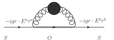
Figure 1: Self energy correction to the singlet propagator Brambilla:2008cx . The singlet state is represented by a single line. The octet by a double line. The vertex is $-igr^{i}$ from the singlet-octet operator $gS^{\dagger}({\bf{r}}\cdot{\bf{E}})O$. At leading order in $g$, the chromo-electric field is $E^{a}=-\partial_{i}A^{a\;0}-\partial_{0}A^{a\;i}$. The blob represent self energy corrections for the gluon.

The simplest analysis arises when weak coupling methods can be applied. For a concrete example, let us review a case considered in Ref. Brambilla:2008cx . We start from NRQCD at the scale $1/r$. The low energy coefficients (LECs) and the propagators at this scale do not have thermal corrections since $1/r\gg T$ and appear at scales comparable to or lower than $T$.

For concreteness let us also assume that the next three scales are $T$, $m_{D}\sim gT$ ($g\ll 1$), and $E_{b}$ in decreasing order. Comparing with the discussion in Sec. 2, one quantity of interest is the (complex) singlet potential. Diagrammatically, this can be calculated by calculating the self energy correction to the singlet propagator from the modes that are integrated out.

The leading (in the multipole expansion) thermal correction is obtained by the dipole terms $gS^{\dagger}({\bf{r}}\cdot{\bf{E}})O+gO^{\dagger}({\bf{r}}\cdot{\bf{E}})S$ in the Lagrangian (Eq. 23). Diagrammatically the correction is shown explicitly in Fig. 1.

The self-energy correction in the static limit (dropping the kinetic energies of the heavy quarks) can simply be written as

$$\delta V_{s}(r)=-ir^{2}T_{F}\int\frac{d^{4}k}{(2\pi)^{4}}\frac{i}{-k^{0}-V_{o}(r)+V_{s}(r)+i\epsilon}[2\tilde{G}_{EE}(k^{0},{\bf{k}})]$$ (24)

Here, $T_{F}=1/2$ is the color Casimir in the fundamental representation $\tilde{G}_{EE}$ is the thermal expectation value of the time ordered chromo-electric correlator

$$\tilde{G}_{EE}(k^{0},{\bf{k}})=\frac{1}{6N_{c}}g^{2}\langle\int d^{4}xe^{i(k^{0}t-{\bf{k}}\cdot{\bf{r}})}{\cal{T}}\{{\bf{E}}^{a}(t,{\bf{r}})W^{ab}(t,{\bf{r}};0,{\bf{0}})\cdot{\bf{E}}^{b}(0,{\bf{0}})\}\rangle_{T}\;.~{}$$ (25)

$W^{ab}$ is the Wilson line in adjoint representation. The $2$ in Eq. 24 arises from the choice of the normalization in Eq. 25.

At the scale $1/r$ $(\gg m_{D})$ the gluonic propagators at the scale $1/r$ can simply be taken to be the vacuum propagator. Therefore at leading order in the coupling, $G_{EE}$ can be obtained from the free propagators Brambilla:2008cx . This gives a real part and also an imaginary part associated with the absorption of on-shell gluons (gluo-dissociation) Peskin:1979 ; Bhanot:1979vb ; Brambilla:2011sg .

At scales lower than $T$, the appropriate propagators for the gluons are the Hard-thermal-loop (HTL) Kapusta:2006pm resummed propagators. The imaginary part of the gluon self energy [associated with the Landau damping of the gluons via interaction with the medium (see Eq. 9 for $q^{0}<q$)] leads to an imaginary contribution to the self energy correction to the singlet propagator. The process is related to the calculation shown above (Sec. 2), where all the fields are expanded in small $r$. This is consistent with the assumed hierarchy ($rE_{b}\ll 1$) used in writing pNRQCD.

Thus we obtain the real and the imaginary parts of the singlet potential, which can be used to calculate the decay rates as described in Sec. 2. The contributions to the complex potential in a framework which includes both the gluo-dissociation and the Landau damping contributions were calculated for the first time in Brambilla:2008cx .

As the above example illustrates, pNRQCD can be used to include all thermal corrections (Landau damping and gluo-dissociation) systematically. Within pNRQCD one can consider different hierarchies between the energy scales $1/r$, $E_{b}$, $T$, and $m_{D}$ and pinpoint the dominant effects in each regime.

For example, it was clarified in Ref. Brambilla:2008cx , that formally the result for the singlet complex potential Eq. 4 is obtained in the limit $1/r\ll T$. It is interesting to note, however, that the form Eq. 4 gives a good description of the singlet potential extracted from the lattice over a wide range of $r$ Burnier:2016mxc .

Assuming $1/r\gg T$ on the other hand, the form of the complex potential depends on the relative order between $T$, $m_{D}$, and $E_{b}$. In the case $T\gg m_{D}\gg E_{b}$ discussed above, there are two contributions to the singlet complex potential: Landau damping and gluo-dissociation (singlet-octet transformation). The Landau damping contribution dominates for $m_{D}\gg E_{b}$ Brambilla:2008cx . The hierarchy $E_{b}\gg m_{D}$ was studied in further detail in Ref. Brambilla:2010vq , and an important result that was found was that the gluo-dissociation contribution was dominant compared to the Landau damping contribution for $E_{b}\gg m_{D}$. Another important point to note is that if the relative order between $T$ and $E_{b}$ is reversed, namely, $T<E_{b}$, then thermal effects do not affect the potential, but arise only when the energy of the state are calculated.

A systematic calculation of gluo-dissociation including $1/N_{c}$ corrections was done in Ref. Brambilla:2011sg and this was extended to dissociation via scattering off light partons in the medium in Ref. Brambilla:2013dpa .

For a detailed discussion of various energy hierarchies that can potentially arise and the relevant physical processes under these different conditions, we refer the reader to the original papers Brambilla:2008cx ; Escobedo:2008sy ; Brambilla:2010vq ; Escobedo:2011ie ; Brambilla:2011sg ; Brambilla:2013dpa ; Brambilla:2011mk

More recently, pNRQCD has been used to derive master equations for the quantum evolution of the density matrix of a ${Q\bar{Q}}$ system in the QGP Brambilla:2016wgg ; Brambilla:2017zei ; Brambilla:2019tpt ; Brambilla:2019oaa . We will discuss these further in Sec. 4.

Another power of the EFT approach is that it provides a tool to go beyond perturbation theory. EFTs often allow us to write observables in a factorized form; a product (or convolution) of a short distance matching coefficient with a long distance matrix element. By matching the correlation functions in the EFT to those in the underlying theory, the matching coefficient can be fixed. This matching can be done perturbatively (which was described above) or non-perturbatively (we will describe an example below). The matrix element can computed within the EFT.

As an illustrative example, consider the case discussed in Ref. Brambilla:2016wgg ; Brambilla:2017zei ; Brambilla:2019tpt ; Brambilla:2019oaa . In the strong coupling limit, the hierarchy $m_{D}\ll T$ is not satisfied and hence the analysis discussed above is not valid. Furthermore, the gluonic propagator is non-perturbative.

However progress can be made in some cases. If we assume that all thermal scales are larger than $E_{b}$, then both the potentials and the kinetic energies of the singlet and octet states can be ignored in Eq. 24, the energy transfer to the medium gluons can be ignored, and the correction to the singlet and octet potentials is determined by $\tilde{G}_{EE}(k^{0}\rightarrow 0,{\bf{k}})$,

$$\delta V_{s}(r)=r^{2}T_{F}\int\frac{d^{3}k}{(2\pi)^{3}}\tilde{G}_{EE}(0,{\bf{k}})\;.$$ (26)

The relevant integral can be simply written in terms of the correlator

$$\begin{split}{G}_{EE}(k^{0}=0,{\bf{r}}={\bf{0}})&=\int\frac{d^{3}k}{(2\pi)^{3}}\tilde{G}_{EE}(0,{\bf{k}})\\ &=\frac{1}{6N_{c}}g^{2}\langle\int dt{\cal{T}}\{{\bf{E}}^{a}(t,{\bf{0}})W^{ab}(t,{\bf{0}};0,{\bf{0}})\cdot{\bf{E}}^{b}(0,{\bf{0}})\}\rangle_{T}\;.~{}\end{split}$$ (27)

The heavy quark momentum diffusion constant of a single heavy quark is proportional to the real part of the chromo-electric correlator $G_{EE}(k^{0}=0,{\bf{r}}={\bf{0}})$ and because of its importance for the phenomenology of open heavy flavor, substantial effort has been put towards its non-perturbative determination. In particular, it has been computed on the lattice Banerjee:2011ra ; Ding:2011hr ; Francis:2015daa ; Brambilla:2019oaa . Recently, an effort has been made to also estimate the imaginary part of the correlator using lattice data Brambilla:2019tpt ; Brambilla:2019oaa .

As another example, there are increasingly sophisticated non-perturbative calculations of the complex singlet potential from the lattice Rothkopf:2011db ; Burnier:2013fca ; Burnier:2014ssa ; Burnier:2015tda ; Burnier:2016mxc ; Bala:2019cqu ; Bala:2019boe .

Non-perturbative calculations of the internal energies and the free energies of a $Q$ and $\bar{Q}$ separated by a distance $r$ at finite temperature were available much earlier Kaczmarek:2002mc ; Kaczmarek:2003ph ; Digal:2003jc ; Kaczmarek:2005ui ; Doring:2007uh . The latter is related to the Polyakov loop correlator McLerran:1981pb . The connection between the Polyakov loop correlators and the singlet and octet potentials were clarified in Refs. Brambilla:2010xn ; Berwein:2012mw ; Berwein:2013xza ; Berwein:2015ayt ; Berwein:2017thy . In this series of papers, it was shown using perturbation theory and pNRQCD that the real part of the singlet potential is well approximated by the singlet free energy. The Polyakov loop and the Polyakov loop correlators were calculated up to $g^{7}$. These correlators were computed on the lattice in Refs. Bazavov:2016uvm ; Bazavov:2018wmo and the results show remarkable agreement with the pNRQCD calculation up to $rT\sim 0.3$.

3 Phenomenology 

Many of these advances in theory have been incorporated in the treatments developed to address the phenomenology of quarkonium states in heavy ion collisions at RHIC and the LHC.

Both experiments have collected data on a number of observables including $R_{AA}$. Another observable that has attracted attention is the collective flow ($v_{2}$) of these states at these facilities. For some results on charmonium at RHIC seeRefs. Adler:2003rc ; Adare:2006ns ; Adare:2008sh ; Abelev:2009qaa ; Adare:2011yf ; Adamczyk:2012pw ; Adamczyk:2012ey ; Adare:2012wf ; Adamczyk:2013tvk ; Aidala:2014bqx ; Adare:2015hva ; Adamczyk:2016srz ; STAR:2019yox ; Adam:2019rbk and at the LHC seeRefs. Chatrchyan:2012np ; Khachatryan:2014bva ; Khachatryan:2016ypw ; Sirunyan:2016znt ; Aad:2010px ; Aad:2010aa ; Aaboud:2018quy ; Aaboud:2018ttm ; Abelev:2012rv ; ALICE:2013xna ; Abelev:2013ila ; Adam:2015rba ; Adam:2015isa ; Adam:2015gba ; Adam:2016rdg ; Acharya:2017tgv ; Acharya:2018jvc ; Acharya:2018pjd ; Acharya:2019iur ; Acharya:2019lkh . For bottomonium states at RHIC see Refs. Adamczyk:2013poh ; Adamczyk:2016dzv ; Adare:2014hje and at the LHC see Refs. Chatrchyan:2011pe ; Khachatryan:2016xxp ; Sirunyan:2017lzi ). These observables have been measured for low as well as high transverse momentum ($p_{T}$) for various centralities and provide important constraints on the models of $Q\bar{Q}$ propagation in the QGP. For a comprehensive review of the observations and phenomenology of quarkonia (and open heavy flavor), see Andronic:2015wma .

The connection from the theoretical calculations of the properties of $Q\bar{Q}$ in a thermal medium to the phenomenology of quarkonia in heavy ion collisions is quite non-trivial.

First, one needs a model for the initial production of the $Q\bar{Q}$ state. The heavy quark pairs are created early in the collisions, on a time scale $\sim 1/(2M)$. It is often assumed that a singlet bound state are formed soon after, on a time scale $1/E_{b}$ in the rest frame of the ${Q\bar{Q}}$. However, one can begin the evolution from a distribution of singlet and octet states Brambilla:2016wgg ; Brambilla:2017zei , which is a natural consequence of the NRQCD formalism Bodwin:1994jh .

The state propagates in a thermal medium that evolves in time, is anisotropic, and features spatial gradients. We assume that a local density approximation still describes the physics: the dissociation rate is given by the instantaneous temperature in the neighbourhood of the ${Q\bar{Q}}$ state.

Let us consider the evolution of ${Q\bar{Q}}$ states moving slowly compared to the ambient medium. Then the formalism described above can be used to calculate the rate. For a pure singlet state $\Psi$, the rate can be obtained from Eq. 16 or Eq. 17. Its calculation involves the knowledge of the wavefunction $\Psi$ at a given instant. Finally, with the dissociation rate in hand, $R_{AA}$ is simply given the probability of survival of the state.

$\Psi$ can be found from the initial state in two extreme approximations, the adiabatic approximation or the sudden approximation. Both approaches have been used in phenomenological applications. We make a note here that neither approximation is expected to work throughout the evolution and it might be more appropriate to describe the ${Q\bar{Q}}$ system as a continuously evolving quantum state using the language of open quantum systems, as we shall discuss below in Sec. 4.

Connection with phenomenology requires taking care of additional effects. Excited states of quarkonia can feed-down to the lower energy states after formation. CNM effects (see Adare:2007gn ; Adler:2005ph ; Adare:2010fn ; Adamczyk:2016dhc ; Abelev:2013yxa ; Abelev:2014zpa ; Abelev:2014oea ; Adam:2015iga ; Adam:2015jsa ; Adamova:2017uhu ; Acharya:2018yud ; Acharya:2018kxc ; Sirunyan:2017mzd ; Aad:2015ddl ; TheATLAScollaboration:2015zdl ; Aaij:2013zxa ) for experimental constraints) modify the initial production rates in $AA$ collisions.

Additionally, as mentioned above, in collisions with high multiplicities of heavy quarks, $Q$ and $\bar{Q}$ from different hard collisions may combine (this is sometimes called coalescence, recombination, or regeneration) to form quarkonia.

Due to the complexity of the problem, there have been various attempts to address the phenomenology, with emphasis on a subset of processes affecting ${Q\bar{Q}}$ propagation in the QGP. We will provide a broad overview of some of these developments below.

1. In Refs. Blaizot:2015hya ; Blaizot:2017ypk ; Blaizot:2018oev the quantum evolution equations for the open ${Q\bar{Q}}$ system were simplified to derive classical transport equations for quarkonia under certain assumptions. The advantage of this approach is that it is not computationally difficult to include the process of coalescence of quarkonia from $Q$, $\bar{Q}$ created in two distinct hard collisions. (This is studied in detail Ref. Blaizot:2017ypk )

2. The possible role of regeneration in quarkonium dynamics was realized early Grandchamp:2001pf ; Grandchamp:2002wp ; Grandchamp:2003 ; Grandchamp:2005yw and this effect has been included at leading order in several studies  Zhao:2007 ; Zhao:2008vu .

   Later, an “in-medium T-matrix” formalism was developed Mannarelli:2005pz ; Cabrera:2006wh for including non-perturbative effects in the interactions between the heavy quarks between each other and between the heavy quarks and the medium particles. (See Ref. vanHees:2007me for the formalism and its application to open heavy flavor.) This was subsequently applied to phenomenology Riek:2010fk ; Zhao:2010nk ; Emerick:2011xu ; Zhao:2012gc ; Liu:2015ypa ; Du:2017qkv ; Liu:2017qah ; Du:2019tjf .

   For other studies including regeneration of quarkonia from coalescence seeRefs. Greco:2003vf ; Zhang:2002ug ; Thews:2006ia ; Bass:2006vu ; Yan:2006ve ; Capella:2007jv ; Bravina:2008su ; Yan:2006ve ; Peng:2010zza ; Ferreiro:2012rq (See BraunMunzinger:2000ep ; Thews:2000rj ; Yan:2006 ; Kostyuk:2003kt ; Thews:2006ia ; Andronic:2011yq ; Gupta:2014ova and references therein for statistical approaches.)

3. In a series of papers Yao:2017fuc ; Yao:2018zze ; Yao:2018nmy ; Yao:2018sgn ; Yao:2020eqy Boltzmann transport equations describing ${Q\bar{Q}}$ evolution were derived and applied to address the phenomenology of bottomonium states. The authors started from the Lindblad equations for ${Q\bar{Q}}$ system treating it as an open quantum system, and derived the Boltzmann equations using some simplifying assumptions

4. In Ref. Hoelck:2016tqf , the gluo-dissociation and the Landau damping contributions to the width were added incoherently and an effect important at large momentum was included: the Doppler shift of the background gluons. In Ref. Hoelck:2017dby the effect of the background electromagnetic field was considered.

5. As discussed above, the QGP is anisotropic. Therefore the formalism developed for screening and damping in homogeneous, isotropic media is not directly applicable there. In a series of papers Dumitru:2007hy ; Dumitru:2009ni ; Dumitru:2009fy ; Strickland:2011mw ; Strickland:2011aa ; Margotta:2011ta ; Machado:2013rta ; Alford:2013jva ; Krouppa:2015yoa ; Krouppa:2016jcl ; Krouppa:2017jlg ; Bhaduri:2018iwr ; Boyd:2019arx , a formalism to include this effect and see its effect on the phenomenology was developed. In Refs. Dumitru:2007hy ; Dumitru:2009ni ; Dumitru:2009fy , the complex color singlet potential in an anisotropic thermal medium was calculated in weak coupling. In Refs. Strickland:2011mw ; Strickland:2011aa ; Margotta:2011ta ; Krouppa:2015yoa ; Krouppa:2016jcl , Eq. 16 was used with the color singlet potential and the adiabatic approximation in an anisotropic thermal medium to calculate $R_{AA}$. Effects due to the magnetic field were considered in Refs. Machado:2013rta ; Alford:2013jva . In Ref. Krouppa:2017jlg the complex singlet potential calculated on the lattice used was the potential at the temperature $T$. In Ref. Bhaduri:2018iwr the formalism was used to calculate $v_{2}$. Deviations from adiabatic evolution were discussed in Ref. Boyd:2019arx .

   The gluo-dissociation contribution to the $T$ dependent potential in an anisotropic medium was computed in pNRQCD in Ref. Biondini:2017qjh .

6. In Song:2005yd ; Park:2007zza ; Song:2007gm (also see Liu:2013kkg ) the leading order calculation of the gluo-dissociation rate by Peskin:1979 ; Bhanot:1979vb was extended to next to leading order. In particular, in Ref. Park:2007zza , dissociation via scattering off light quarks and gluons in the medium were treated in a unified framework. [This calculation was further extended using the EFT framework in Ref. Brambilla:2013dpa (see Sec. 2.1).]

   Assuming that gluo-dissociation is the dominant decay process for quarkonia, quarkonium observables were calculated in Refs. Song:2010ix ; Song:2010er ; Song:2011nu ; Song:2011xi . Additional effects on the formation dynamics of quarkonia were discussed in Refs. Song:2013lov ; Lee:2013dca ; Song:2014qoa ; Song:2015bja

7. More recently, the theory of open quantum systems in the framework of pNRQCD has been applied to the phenomenology of bottomonia in Refs. Brambilla:2016wgg ; Brambilla:2017zei .

After this broad overview of various approaches used for quarkonium phenomenology, we now describe in some more detail a calculation of $R_{AA}$ done in Ref. Aronson:2017ymv for high $p_{T}$ quarkonia and comparison with the observations at the LHC.

3.1 Quarkonia at high $p_{T}$ 

For high $p_{T}$ ($p_{T}\gtrsim 2M$) quarkonia, it may be more appropriate to start from a formalism used to study the propagation of highly energetic partons in the quark gluon plasma. In this section, we will review results from Ref. Aronson:2017ymv which applies this formalism to the calculation of $R_{AA}$ for quarkonia with large $p_{T}$.

The formalism is based on solving the rate equations for $Q\bar{Q}$ pairs. The physical picture is simple. $Q\bar{Q}$ pairs with large transverse momenta, correlated over short distances are produced in hard processes. These form quarkonium states over a time scale $t_{\rm{form.}}$. Collisions with the medium gluons lead to the dissociation of quarkonium states over a time scale $t_{\rm{diss.}}$. Mathematically, the differential cross-sections for the $Q\bar{Q}$ states and the quarkonia evolve according to,

$$\begin{split}\frac{d}{dt}\left(\frac{d\sigma^{Q\bar{Q}}(t;p_{T})}{dp_{T}}\right)&=-\frac{1}{t_{\rm form.}}\frac{d\sigma^{Q\bar{Q}}(p_{T})}{dp_{T}}\,,\\ \frac{d}{dt}\left(\frac{d\sigma^{\rm meson}(t;p_{T})}{dp_{T}}\right)&=\frac{1}{t_{\rm form.}}\frac{d\sigma^{Q\bar{Q}}(t;p_{T})}{dp_{T}}\\ &-\frac{1}{t_{\rm diss.}}\frac{d\sigma^{\rm meson}(t;p_{T})}{dp_{T}}\,.\end{split}$$ (28)

Solving Eq. 28 for each $p_{T}$ requires the initial conditions of the differential yields and the knowledge of $t_{\rm diss.}$ and $t_{\rm form.}$. We discuss each of these below.

The production of high $p_{T}$ $Q\bar{Q}$ states is given by the NRQCD formalism Bodwin:1994jh . The cross-sections for quarkonium production in $pp$ collisions can be formally written as

$$d\sigma(ij\rightarrow{\rm{meson}}+X)(p_{T})=\sum_{n}d\sigma(ij\rightarrow Q\bar{Q}[n]+X^{\prime})(p_{T})\langle{\cal{O}}[n]\rangle\;,~{}$$ (29)

where $i,\;j$ refer to initial partons (primarily $gg$ at the LHC). $d\sigma(ij\rightarrow Q\bar{Q}[n]+X^{\prime})(p_{T})$ refer to short distance coefficients for the production of $Q\bar{Q}$ in a particular color (for example singlet or octet) and angular momentum (${}^{2S+1}L_{J}$) configuration which we collectively label as $[n]$ for short here. These coefficients can be computed in perturbation theory (See Refs. Baier:1983 ; Humpert:1987 ; Cho:1995ce ; Cho:1995vh ; Braaten:2000cm ; Sridhar:1996vd for the computation to the NLO. See Refs. Butenschoen:2010rq ; Butenschoen:Long ; Butenschoen:polarised ; Wang:2012is ; Shao:2014yta for NNLO computations.) $\langle{\cal{O}}[n]\rangle$ refer to long distance matrix elements (LDMEs) which correspond to the probability of forming a particular mesonic state (for example $J/\psi$, $\psi(2S)$, $\chi_{cJ}^{1}$, or $\chi_{cJ}^{2}$ states for $c\bar{c}$) from the short distance $Q\bar{Q}$ states. These have to be fitted to experimentally observed $p_{T}$ differential yields for the various mesons. We used the fit in Ref. Sharma:2012dy .

In $AA$ collisions, Eq. 29 does not give the final meson yields due to two reasons. First, the formed states can be dissociated by the medium (final state effects). These are handled by Eq. 28. Thus the left hand side of Eq. 29 only gives the initial state for $\frac{d\sigma^{Q\bar{Q}}(t;p_{T})}{dp_{T}}$ in Eq. 28 . The initial value of $\frac{d\sigma^{\rm{meson}}(t;p_{T})}{dp_{T}}$ is $0$. Second, the production cross-sections $d\sigma(ij\rightarrow Q\bar{Q}[n]+X^{\prime})(p_{T})$ are themselves modified due to initial state (CNM) effects. These can be estimated by measuring the modification factor $pA$ collisions. For charmonia at low $p_{T}$ CNM effects are substantial for forward and backward rapidity Abelev:2013yxa ; Abelev:2014zpa ; Adam:2015iga ; Adam:2015jsa , they seem to be consistent with a small ($\sim 10\%$ for prompt $J/\psi$ and even smaller for $\psi(2S)$) enhancement for $p_{T}>5$ GeV at central rapidities in $p{\rm{Pb}}$ collisions Sirunyan:2017mzd . For $\Upsilon(1s)$ at central rapidity, results are consistent with absence of CNM effects TheATLAScollaboration:2015zdl . In our calculation we will ignore these effects.

The second ingredient in Eq. 28 is the dissociation time. Intuition from the study of high $p_{T}$ partons suggests that an important process is transverse momentum broadening: the energetic parton picks up momentum perpendicular to its motion due to random kicks from thermal gluons in the medium. Detailed formalisms to calculate this effect have been developed (see Refs. Baier:1996sk ; Zakharov:1996fv ; Baier:1998kq ; Gyulassy:1999zd ; Gyulassy:2000er ; Wiedemann:2000za and references therein).

For a time independent medium at the temperature $T$, an energetic parton traversing a distance $L$ accumulates momentum transverse to its motion. In weak coupling, assuming that scattering in the medium can be effectively modelled by $T$ channel scattering off static colored sources, the opacity $\chi=L/\lambda$ ($\lambda$ is the mean free path of the parton) is substantially larger than $1$, the distribution of the net momentum transfer ($q_{T}$) to a single energetic quark transverse to its motion can be approximated Gyulassy:2002yv ; Wiedemann:2000za ; Adil:2006ra by

$$\frac{d{\cal{P}}({\bf{q}}_{T})}{d{\bf{q}}_{T}}\sim e^{-\frac{{\bf{q}}_{T}^{2}}{2\chi m_{D}^{2}\xi}}~{}$$ (30)

$\xi\gtrsim 1$ is a parameter that roughly accounts for the fact in transverse impact parameter space (the Fourier conjugate of ${\bf{q}}_{T}$), the small impact parameter expansion receives logarithmic corrections. (If the exchanges are strictly very soft, $\xi=1$). $m_{D}$ is the screening mass of the exchanged gluons with the medium. Eq. 30 describes momentum broadening with a broadening parameter $\hat{q}={2\chi m_{D}^{2}\xi}$.

For an energetic $Q\bar{Q}$ pair moving together in the medium, the transverse momentum transfers lead to a distortion of the state in transverse momentum space and lead to the dissociation of bound states. This idea was first used to propose a new energy loss mechanism for $D$ and $B$ mesons Adil:2006ra . (See also Sharma:2009hn .)

In Refs. Sharma:2012dy ; Aronson:2017ymv this was applied to the study of quarkonium propagation in the medium. Here, we follow the effect of broadening on a state of of the $Q$ and $\bar{Q}$ Aronson:2017ymv .

The analysis of transverse broadening of energetic $Q\bar{Q}$ states can be nicely done by writing the states as light cone wavefunctions. The lowest Fock states consist of $Q\bar{Q}$ in the color singlet configuration. In this approximation the heavy meson state of momentum $\vec{P^{+}}=(P^{+},{\bf P})$ can be approximated as:

$$|\vec{P}^{+}\rangle = \int\frac{d^{2}{\bf k}}{(2\pi)^{3}}\frac{dx}{2\sqrt{x(1-x)}}\frac{\delta_{c_{1}c_{2}}}{\sqrt{3}}\,\psi(x,{\bf k})$$ (31)

$$\times a_{Q}^{\dagger\;c_{1}}(x\vec{P}^{+}+{\bf k})b_{\bar{Q}}^{\dagger\;c_{2}}((1-x)\vec{P}^{+}-{\bf k})|0\rangle\;,$$

where $a^{\dagger}$ ($b^{\dagger}$) represent an “effective” heavy quark (anti-quark) in the $3$ ($\bar{3}$) state, $c_{1},c_{2}$ being the color indices Sharma:2009hn ; Sharma:2012dy .

The light cone wavefunction in momentum space has the form,

$$\psi(x,{\bf k})={\rm Norm}\times\exp\left(-\frac{{\bf k}^{2}+m_{Q}^{2}}{2\Lambda^{2}(T)x(1-x)}\right)\;,$$ (32)

where the normalization is given by the relation,

$$\frac{1}{2(2\pi)^{3}}\int dxd^{2}{\bf k}\;|\psi(x,{\bf k})|^{2}=1\;.$$ (33)

$x$ refers to the longitudinal fraction of the momentum. ${\bf k}$ refers to the transverse momentum.

The transverse extent of the states

$$\frac{1}{2(2\pi)^{3}}\int dxd^{2}{\bf k}\;{\Delta\bf k}^{2}|\psi(x,{\bf k})|^{2}=4\langle{\bf k^{2}}\rangle=\frac{2}{3}\kappa^{2}\;.$$ (34)

To be concrete, let us follow the evolution of the $Q\bar{Q}$ state created in a hard collision (early time) at a transverse location ${\bf x}_{0}$ (we will focus on central rapidity) for a state that propagates with velocity ${\bf\beta}$, such that ${\bf x}(\tau)={\bf x}_{0}+{\bf\beta}(\tau-t_{0})$. The temperature changes as the system evolves and the state moves and we call the instantaneous value as $T$. The evolution is started at $t=t_{0}$ which is taken to be $t_{0}=0.6$fm. By this time the medium is likely to be thermalized and a hydrodynamic description is possible. (For reviews of hydrodynamic simulations see Romatschke:2009im ; Teaney:2009qa ; Hirano:2012qz ; Song:2013gia ; Gale:2013da ; Shen:2014vra ; Jeon:2015dfa ; Jaiswal:2016hex .)

After traversing the medium for a time $t$, the cumulative relative transverse dimensional momentum transfer reads

$$\chi m_{D}^{2}\xi=\int_{t_{0}}^{t}d\tau\frac{m_{D}^{2}(\bf{x}(\tau),\tau)}{\lambda_{q}({\bf x}(\tau),\tau)}\xi\,,$$ (35)

Here we use $N_{f}=2$. The scattering inverse length of the quark is ${1}/{\lambda_{q}}=\sigma_{qq}\rho_{q}+\sigma_{qg}\rho_{g}$, where $\rho_{q}$ and $\rho_{g}$ are the partial densities of light quarks and gluons in the QGP. The elastic scattering cross sections are given by

$$\sigma_{qq}=\frac{1}{18\pi}\frac{g^{4}}{m_{D}^{2}}\,,\quad\sigma_{qg}=\frac{1}{8\pi}\frac{g^{4}}{m_{D}^{2}}\,.$$ (36)

We initialize the wavefunction $\psi_{i}(\Delta{\bf k},x)$ of the proto-quarkonium $Q\bar{Q}$ state with a width $\Lambda_{0}\equiv\Lambda(T=0)$. This is a natural choice since in the absence of a medium it will evolve on the time-scale of ${\cal O}(1{\rm fm})$ into the observed heavy meson. By propagating in the medium this initial wavefunction accumulates transverse momentum broadening $\chi m_{D}^{2}\xi$. The probability that this $Q\bar{Q}$ configuration will transition into a final-state heavy meson with thermal wavefunction $\psi_{f}(\Delta{\bf k},x)$ with $\Lambda(T)$ is given by

$$\begin{split}P_{f\leftarrow i}(\chi m_{D}^{2}\xi,T)&=\left|\frac{1}{2(2\pi)^{3}}\int d^{2}{\bf k}dx\,\psi_{f}^{*}(\Delta{\bf k},x)\psi_{i}(\Delta{\bf k},x)\right|^{2}\\ &=\left|\frac{1}{2(2\pi)^{3}}\int dx\;{\rm Norm}_{f}{\rm Norm}_{i}\,\pi\,e^{-\frac{m_{Q}^{2}}{x(1-x)\Lambda(T)^{2}}}e^{-\frac{m_{Q}^{2}}{x(1-x)\Lambda_{0}^{2}}}\right.\\ &\times\left.\,\frac{2[x(1-x)\Lambda(T)^{2}][\chi m_{D}^{2}\xi+x(1-x)\Lambda_{0}^{2}]}{[x(1-x)\Lambda(T)^{2}]+[\chi m_{D}^{2}\xi+x(1-x)\Lambda_{0}^{2}]}\;\right|^{2}\,.\;\;\quad\end{split}$$ (37)

In Eq. (37) ${\rm Norm}_{i}$ is the normalization of the initial state, including the transverse momentum broadening from collisional interactions, and ${\rm Norm}_{f}$ if the normalization of the final state.

The dissociation rate for the specific quarkonium state can then be expressed as

$$t_{\rm diss.}=-\frac{1}{P_{f\leftarrow i}(\chi m_{D}^{2}\xi,T)}\frac{dP_{f\leftarrow i}(\chi m_{D}^{2}\xi,T)}{dt}\,.$$ (38)

Finally, the third ingredient we need is the formation time $t_{\rm form.}$. In various studies this was taken to be $\sim\gamma\frac{1}{E_{b}}$ (where $\gamma$ takes care of the time dilation). Here we consider it as a parameter which we vary between $1$fm to $1.5$fm. The intuition behind this choice is that for the thermal wavefunction, $\tau_{f}$ refers to the time scale on which a proto-quarkonuim ${Q\bar{Q}}$ state is affected more by the medium and is dependent on the medium properties like $T$ than the boost of the ${Q\bar{Q}}$ state.

With all the ingredients in place, we evolve using Eq. 28 in a medium which is given by a solution of the hydrodynamic equations. This is taken from the publicly available iBNE-VISHNU implementation of hydrodynamics Shen:2014vra with Glauber initial states. The distribution of the hard collisions is given by the distribution of binary collisions in the Glauber model. In the azimuthal direction, the $p_{T}$ momentum direction is isotropic.

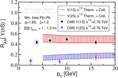
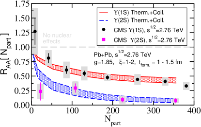
Figure 2: $R_{AA}$ versus $p_{T}$ (left panel) and $N_{\rm{part}}$ (right panel) for PbPb collisions at $2.76$TeV at the LHC for $\Upsilon$ states.

Solving Eq. 28 for each of the mesonic states gives the $p_{T}$ differential yields for them. Finally, after taking into account the feed-down from the excited states to the ground states we can find the final $p_{T}$ differential yields in $AA$ collisions.

Dividing the yields in $AA$ with the normalized yields in $pp$ gives $R_{AA}$. In the next section, we show the results from our calculation for at the LHC.

3.2 Results

We now show a set of illustrative results of the calculation and comparisons with the observations.

First considering the $\Upsilon$ states, we show results as a function of $p_{T}$ as well as $N_{\rm{part}}$ in Fig. 2. We show similar results for charmonia in Fig. 3. One nice feature is both $J/\psi$ and $\Upsilon$ ground states and the first excited states are described by the model. Both screening and dissociation play a role in getting the relative suppression between the two.

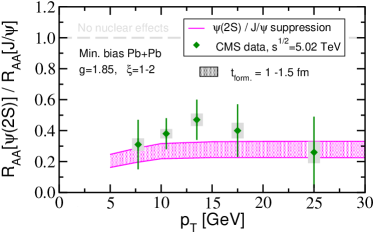
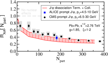
Figure 3: The relative suppression of $J/\psi$ and $\psi(2s)$ versus $p_{T}$ in $5.02$TeV PbPb collisions (left panel) and $R_{AA}$ versus $N_{\rm{part}}$ (right panel) in $2.76$TeV PbPb collisions for $J/\psi$ at the LHC

Looking ahead, one can think of improvements to the calculation. First, the largest systematic uncertainty in the calculation comes from the ignorance about the formation dynamics. These have been parameterized by a single parameter in the model, $t_{\rm{form}}$. Reducing this uncertainty will require modelling the conversion of the short distance color-singlet and color-octet states to a bound color singlet state. Second, the treatment of the color degrees of freedom in the model above was too simplified. A recently developed EFT Makris:2019ttx ; Makris:2019kap for the propagation of high $p_{T}$ quarkonia in the QGP provides a framework in which the color structure and the proper kinematics of the relevant modes can be systematically treated. Finally, the dynamics described here are given by rate equations which miss the coherent evolution of the ${Q\bar{Q}}$ state. As we discuss below, in a simple example, these quantum effects might be important in a rapidly evolving QGP.

4 Quarkonia in the QGP as open quantum systems 

In the phenomenological applications discussed above, the dissociation rate for quarkonia are given by the form

$$\Gamma\sim\sum_{f}\overline{|\langle\Psi|\hat{O}|f\rangle|}^{2}~{}$$ (39)

where $\hat{O}$ is a transition operator $|f\rangle$ refers to a dissociated state. For example, $\hat{O}={\bf{E}}\cdot{\bf{r}}$ and $|f\rangle$ correspond to color-octet states in the case of gluo-dissociation. The overline corresponds to taking a thermal expectation value.

In a time independent medium, this gives the leading order (in $\hat{O}$) decay rate for an initial state $|\Psi\rangle$ which is typically chosen to be the quarkonium wavefunction in vacuum.

However, in a time dependent medium, there are additional effects. As discussed above, both the real and imaginary parts of the complex potential depend on time. Even so, there are two cases where Eq. 39 gives the instantaneous decay rate in the medium.

The first case is when the background potential changes very rapidly compared to the energy difference between levels ($\Delta E$) of the system. Then an “instant” formalism can be used and $|\Psi\rangle$ can be taken as the vacuum state at any given time. The other case is when the background potential changes very slowly, and one can assume that $|\Psi\rangle$ represents the eigenstate of the instantaneous potential (adiabatic approximation) Dutta:2012nw .

For Bjorken evolution, the rate of change is $\sim\frac{1}{T}\frac{dT}{dt}=-\frac{1}{3\tau}$. In the absence of a clear hierarchy between $1/\tau$ and $\Delta E$, one needs to follow the quantum state as the medium evolves, while keeping track of the exchange of energy and momentum between the state and the medium. The theory of open quantum systems commonly used in the study of non-equilibrium condensed matter systems Breuer:2002pc provides such a formalism.

In this formalism, the system is described by the density matrix ($\rho$) of the ${Q\bar{Q}}$ state obtained by tracing out the environmental degrees of freedom. The evolution of $\rho$ is described by master equations  Akamatsu:2011se ; Akamatsu:2012vt ; Akamatsu:2013 ; Akamatsu:2015kaa ; Kajimoto:2017rel ; Akamatsu:2018xim ; Miura:2019ssi ; Brambilla:2016wgg ; Brambilla:2017zei ; Brambilla:2019tpt ; Brambilla:2019oaa ; Blaizot:2018oev obtained after this tracing procedure. (See Ref. Akamatsu:2020ypb for a recent review.)

There are two regimes explored widely in the literature Breuer:2002pc ; Akamatsu:2013 . One is when the system relaxation time is longer than $1/\Delta E$. This is known as the quantum optical limit. The second case is when the system relaxation time is shorter than $1/\Delta E$. This is known as the quantum Boltzmann limit. It is typically assumed that the relaxation time for the environment is short compared to the system relaxation time, otherwise the evolution equations at a given instant depend on the full history of the evolution: i.e. the equations are not Markovian. [In the presence of long lived excitations in the environment the Markovian approximation may be violated. (See Sec. 4.1.)]

In the quantum optical regime, a convenient basis for $\rho$ is the eigenstates of the system Hamiltonian. Interactions with the environment lead to transitions between the states as well as transitions out of the Hilbert space of bound states. This formalism was used to write master equations for the system density matrix in terms of the transition rates between the states and calculate the relative yields of $c\bar{c}$ and $b\bar{b}$ states in Ref. Borghini:2011yq ; Borghini:2011ms . This approach is of particular interest for $b\bar{b}$ states in the QGP if they “survive” for temperatures sufficiently above the crossover temperature.

In the quantum Boltzmann regime, it is more convenient to write the density matrix in the position basis. A model where a ${Q\bar{Q}}$ interacting with an environment with an ohmic spectral function was discussed in Ref. Young:2010jq . The authors wrote the formal expression for the system density functional in terms of a path integral. They subsequently used Monte Carlo techniques to integrate out the environment numerically and calculated the Euclidean current-current correlation function $\bar{\psi}\gamma^{\mu}\psi(\tau,{\bf{r}})\bar{\psi}\gamma^{\mu}\psi(0,0)$. (This is closely related to ${\cal{C}}(q^{\mu})$ defined in Eq. 1.)

In general, the process of explicitly tracing out the environmental degrees is complicated. However, evolution equations for the ${Q\bar{Q}}$ density matrix evolution using two different approaches.

One approach was developed in a series of papers Akamatsu:2011se ; Akamatsu:2012vt ; Akamatsu:2013 ; Akamatsu:2015kaa ; Kajimoto:2017rel ; Akamatsu:2018xim ; Miura:2019ssi , in which master equations for the density matrices for isolated heavy quarks and ${Q\bar{Q}}$ pairs were derived and applied in weak coupling. We summarize an important result from Ref. Akamatsu:2013 relevant for Sec. 4.1 and refer the reader to the original papers for more details.

The key assumptions in deriving the master equations are

1. The strong coupling $g$ is assumed to be small. Thus the real part of the ${Q\bar{Q}}$ potential has the screened Coulomb form. Furthermore, the gluonic propagators are replaced by the weak coupling form (for eg. Eq. 9).

2. It was assumed that $E_{b}\ll m_{D}$ (consistent with the quantum Boltzmann regime)

3. Furthermore, we will focus on the regime where quantum dissipation does not play an important role. This corresponds to dropping ${\cal{O}}(v)$ and ${\cal{O}}(v^{2})$ terms in the path integral used to derive the master equation  Akamatsu:2015kaa and can be formally justified if $v$ is small. However dissipation can have important quantitative effects Miura:2019ssi

Under these approximations, the master-equation for the ${Q\bar{Q}}$ pair can be written in Lindblad form Akamatsu:2015kaa ; Lindblad:1975ef

$$\frac{\partial}{\partial t}\left(\begin{array}[]{c}{\rho_{1}}\\ {\rho_{8}}\end{array}\right)_{(t,\vec{r},\overline{s})} = \left(i\frac{\vec{\nabla}_{r}^{2}-\vec{\nabla}_{s}^{2}}{M}\right)\left(\begin{array}[]{c}{\rho_{1}}\\ {\rho_{8}}\end{array}\right)_{(t,\vec{r})}+i(V(\vec{r})-V(\vec{s}))\left[\begin{array}[]{cc}{C_{\mathrm{F}}}&{0}\\ {0}&{-1/2N_{\mathrm{c}}}\end{array}\right]\left(\begin{array}[]{c}{\rho_{1}}\\ {\rho_{8}}\end{array}\right)_{(t,\vec{r},\vec{s})}$$ (51)

$$+{\mathcal{D}}(\vec{r},\vec{s})\left(\begin{array}[]{c}{\rho_{1}}\\ {\rho_{8}}\end{array}\right)_{(t,\vec{r},\vec{s})}.$$

Here $\vec{r}$ corresponds to the relative separation between the ${Q\bar{Q}}$ in the “ket” space and $\vec{s}$ is the separation in the “bra” space. $\rho_{1,\;8}=\rho_{1,\;8}(t,\vec{r},\vec{s})$ are the singlet and octet components of the ${Q\bar{Q}}$ density matrix in position space. $V(\vec{r}),V(\vec{s})$ correspond to the potential between $Q$ and $\bar{Q}$. We consider the ${Q\bar{Q}}$ pair at rest in the medium and hence the center-of-mass coordinates $\vec{R}$, $\vec{S}$ do not play a role and we have suppressed the dependence on them.

${\mathcal{D}}(\vec{r},\vec{s})$ are terms related to decoherence of the ${Q\bar{Q}}$ state Akamatsu:2015kaa ,

$$\begin{split}{\mathcal{D}}(\vec{r},\vec{s})=&2C_{\mathrm{F}}D(\overrightarrow{0})-(D(\vec{r})+D(\vec{s}))\left[\begin{array}[]{cc}{C_{\mathrm{F}}}&{0}\\ {0}&{-1/2N_{\mathrm{c}}}\end{array}\right]-2D\left(\frac{\vec{r}-\vec{s}}{2}\right)\left[\begin{array}[]{cc}{0}&{1/2N_{\mathrm{c}}}\\ {C_{\mathrm{F}}}&{C_{\mathrm{F}}-1/2N_{\mathrm{c}}}\end{array}\right]\\ &+2D\left(\frac{\vec{r}+\vec{s}}{2}\right)\left[\begin{array}[]{cc}{0}&{1/2N_{\mathrm{c}}}\\ {C_{\mathrm{F}}}&{-1/N_{\mathrm{c}}}\end{array}\right].\end{split}$$ (52)

The function $D(\vec{r})$ is related to the imaginary part of gluonic self-energy. In the HTL approximation,

$$D(\vec{r})=-g^{2}T\int\frac{d^{3}k}{(2\pi)^{3}}\frac{\pi m_{\mathrm{D}}^{2}e^{i\vec{k}\cdot\vec{r}}}{k\left(k^{2}+m_{\mathrm{D}}^{2}\right)^{2}}\;.$$ (53)

One can immediately identify $D(\vec{r})$ as the Fourier transform of the small $q^{0}$ form of the longitudinal gluonic spectral function multiplied by $n_{B}(q^{0})$ (Eqs. 12, 14).

Eq. 51 can be solved by introducing noise fields $\theta^{a}(t,\vec{r})$ Akamatsu:2015kaa which are picked from an ensemble which is specified by the following expectation values,

$$\langle\langle\theta^{a}(t,\vec{r})\rangle\rangle = 0$$

$$\langle\langle\theta^{a}(t,\vec{r})\theta^{b}(t^{\prime},\vec{r}^{\prime})\rangle\rangle = \delta^{ab}D(\vec{r}-\vec{r}^{\prime})\delta(t-t^{\prime})\;,$$ (54)

where $\langle\langle..\rangle\rangle$ signifies taking the stochastic average over the noise fields.

For each member of the ensemble $\theta^{a}(t,\vec{r})$, $\psi$ is evolved using the Schrödinger equation,

$$\psi(t+dt) =e^{-iH_{\theta}(t)dt}\psi(t)$$

$$H_{\theta}(\vec{r},t) =-\frac{\vec{\nabla}_{r}^{2}}{M}+V(r)(t^{a}\otimes t^{a,\ast})+\theta^{a}(t,\frac{\vec{r}}{2})\left(t^{a}\otimes 1\right)-\theta^{a}(t,-\frac{\vec{r}}{2})\left(1\otimes t^{a*}\right).\;$$ (55)

The density matrix can be obtained by taking a stochastic average of the outer product

$$\rho(t,\vec{r},\vec{s})=\langle\langle\;\;\ket{\psi(t,\vec{r})}\bra{\psi(t,\vec{s})}\;\;\rangle\rangle\;.$$ (56)

A simplified version of Eq. 4 was simulated in Akamatsu:2018xim , where the wavefunction was assumed to be one-dimensional and the color-structure of ${Q\bar{Q}}$ pair was neglected. In Sharma:2019xum the calculation was extended to include the full color structure and three dimensional wavefunction. In addition the evolution was extended to noise correlated in time. We will describe this work in Sec. 4.1.

The second approach was developed in a series of papers Brambilla:2016wgg ; Brambilla:2017zei ; Brambilla:2019tpt ; Brambilla:2019oaa . The authors started from the pNRQCD lagrangian (Eq. 23). At the leading order in the multipole expansion, the evolution of the singlet and the octet components of density matrix are given by the singlet and the octet hamiltonians respectively. The first order correction arises due to the dipole term. The diagrams are similar to Fig. 1 where the propagators now refer to the propagation of the density matrix in time. (See Refs. Brambilla:2016wgg ; Brambilla:2017zei for the details of the calculation.)

Refs. Brambilla:2016wgg ; Brambilla:2017zei were the first papers to include both gluo-dissociation and Landau damping in a consistent framework taking into account the full non-Abelian and quantum nature of the problem of a ${Q\bar{Q}}$ propagating in a thermal medium. This approach conserves the number of $Q$ and $\bar{Q}$ during the evolution. At the same time, since the evolution maintains the coherence, both “dissociation” and “recombination” occur during evolution. Finally, it has the advantage that various hierarchies between $T$, $m_{D}$, and $E_{b}$ can be considered.

In Refs. Brambilla:2016wgg ; Brambilla:2017zei ; Brambilla:2019tpt ; Brambilla:2019oaa , it was shown that in the hierarchy $1/r\gg\pi T\sim m_{D}\gg E_{b},\;\Lambda_{QCD}$, the master equations at a given $T$ are specified by only two constants, $\kappa$ and $\gamma$, the $\Re e$ and the $\Im m$ parts of the chromo-electric field correlator (Eq. 27).

In Refs. Brambilla:2016wgg ; Brambilla:2017zei this technique was applied to the phenomenology of bottomonia at LHC by calculating $R_{AA}$ for $\Upsilon(1S)$ and $\Upsilon(2S)$ states (see Fig. $7$ in Ref. Brambilla:2017zei ).

4.1 Correlated and uncorrelated noise 

We first simplify the stochastic evolution equation (Eq. 4) (and therefore its corresponding master equation) by expanding the decoherence terms in small $\vec{r},\vec{s}$. This approximation is motivated by the hierarchy between the inverse size of the states and the temperature $1/r\gg T$.

This allows us to extend the calculation to a three dimensional system while keeping all the color structure of ${Q\bar{Q}}$ pair intact without a high computational cost. The calculation allows for transitions between different angular-momentum states ($l=0,1$). Transitions which change the angular-momentum by two units or more are suppressed Brambilla:2016wgg ; Brambilla:2017zei by ${\mathcal{O}}(r^{2}T^{2})$.

The stochastic evolution operator up to ${\mathcal{O}}(\vec{r}^{2})$ for a $l=0$ initial state is,

$$\psi(t+dt)=e^{-iH_{\theta}dt}\psi(t)$$

$$H_{\theta}=(\frac{-\nabla^{2}}{M}(1_{Q}\otimes 1_{\bar{Q}})+V(r)(t^{a}\otimes t^{\ast,a})+D^{a}\ \frac{\vec{r}}{2}\cdot\vec{\theta}^{a}(t)+F^{a}\ \theta^{a}(t)+\mathcal{O}(\vec{r}^{2}))$$

$$\theta^{a}(t)=\theta^{a}(\vec{r},t)|_{\vec{r}=0},\quad\vec{\theta}_{i}(t)=\vec{\nabla}_{i}\theta(\vec{r},t)|_{\vec{r}=0}\;,$$ (57)

where the noise field $\theta(\vec{r},t)$ was defined in Eq. 4. ($F^{a}=(t^{a}_{Q}\otimes 1_{\bar{Q}}-1_{Q}\otimes t^{\ast\;a}_{\bar{Q}})$ and $D^{a}=(t^{a}_{Q}\otimes 1_{\bar{Q}}+1_{Q}\otimes t^{\ast\;a}_{\bar{Q}})$ are operators in the color-space of ${Q\bar{Q}}$ pair. The subscript $i$ refers to the spatial index, and we refer $\vec{\nabla}_{i}\theta({\bf{r}},t)|_{{\bf{r}}=0}$ as the three tuple $\theta_{i}(t)$ for notational convenience.)

The noises appearing in Eq. 4.1 can be generated as random-fluctuations uncorrelated at unequal times,

$$\langle\langle{\theta}^{a}_{i}(t)\rangle\rangle = 0$$

$$\langle\langle\vec{\theta_{i}}^{a}(t)\vec{\theta_{j}}^{b}(t^{\prime})\rangle\rangle = \delta^{ab}\delta(t-t^{\prime})\delta_{ij}\frac{-\nabla^{2}}{3}D(\vec{0}).$$ (58)

The noise $\vec{\theta_{i}}^{a}(t)$ can be interpreted as the $gE^{i\;a}(t)$ at the center of mass of the $Q$ and $\bar{Q}$, and $-\frac{1}{3}\nabla^{2}D$ is simply the chromo-electric correlator. The noise correlated only at equal time and this is reminiscent of the static limit discussed in Sec. 2. This is a direct consequence of the assumption that $E_{b}\ll m_{D}$: the system evolution is slow compared to the relaxation and hence the noise is uncorrelated at unequal times.

The above Hamiltonian evolution is written for a three dimensional system. Since, $V(\vec{r})$ is rotationally invariant, we can separate the radial part of the three dimensional wavefunction from its angular part. The wavefunction in position space can be written as

$$\Psi(\vec{r},t)=\frac{\psi(r)}{r}\Theta(\beta,\phi),$$ (59)

where $\psi(r)$ is the radial wavefunction and $\Theta$ is the wavefunction in angular momentum space, with $\beta$ being the polar angle and $\phi$ azimuthal angle. We also define the normalized color states for ${Q\bar{Q}}$ octet and singlet wavefunction as,

$$\ket{S}=\frac{1}{\sqrt{N_{c}}}\sum_{lk}\ket{lk}\quad\ket{O^{a}}=\frac{1}{\sqrt{T_{F}}}\sum_{lk}(t^{a})_{lk}\ket{lk}.$$ (60)

The indices $l,k$ denotes the color states of a single quark or antiquark.

Finally, we project the evolution operator in the Eq. 4.1 into the color and angular momentum space of ${Q\bar{Q}}$ pair,

$$H_{\theta}(r,t)=\left(\begin{array}[]{cccc}H^{S}_{0}(r,t)&0&0&\frac{1}{\sqrt{2N_{c}}}r|\vec{\theta}^{c}(t)|\delta_{ac}\\ 0&H^{S}_{1}(r,t)&\frac{1}{\sqrt{2N_{c}}}r|\vec{\theta}^{c}(t)|\delta_{ac}&0\\ 0&\frac{1}{\sqrt{2N_{c}}}r|\vec{\theta}^{c}(t)|\delta_{ac}&H^{O}_{0}(r,t)+f^{abc}\theta^{c}(t)&\frac{d^{abc}}{2}r|\vec{\theta}(t)|\\ \frac{1}{\sqrt{2N_{c}}}r|\vec{\theta}^{a}(t)|\delta_{ac}&0&\frac{d^{abc}}{2}r|\vec{\theta}(t)|&H^{O}_{1}(r,t)+f^{abc}\theta^{c}(t)\end{array}{}\right).$$ (61)

This Hamiltonian acts on the wavefunction given in the form

$$\psi(r,t)=\left(\psi^{S}_{l=0}(r,t),\psi^{S}_{l=1}(r,t),\psi^{O^{a}}_{l=0}(r,t),\psi^{O^{a}}_{l=1}(r,t)\right).$$ (62)

Here, $\psi^{S}(r,t)$ and $\psi^{O^{a}}(r,t)$ denote radial wavefunctions for ${Q\bar{Q}}$ pair in singlet and octet states respectively and the index $a$ runs from $1$ to $(N_{c}^{2}-1)$ for different color-octet states. $l$ denotes the angular momentum states, which take the values $l=0,1$. The Hamiltonians for the singlet and octet states are

$$H^{S}_{l} =-\frac{1}{M}\frac{\partial^{2}}{\partial r^{2}}-\frac{C_{\mathrm{F}}\alpha}{r}e^{-m_{D}r}+\frac{l(l+1)}{Mr^{2}},$$

$$H^{O}_{l} =-\frac{1}{M}\frac{\partial^{2}}{\partial r^{2}}+\frac{\alpha}{2N_{\mathrm{c}}r}e^{-m_{D}r}+\frac{l(l+1)}{Mr^{2}}.$$ (63)

Under the approximations considered, the correlation functions (Eqs. 4.1) are the most important quantities which control the suppression pattern. As discussed above, when $E_{b}\ll m_{D}$ the noise correlator is local in time (Eqs. 4, 4.1). When this hierarchy is not satisfied, the noise terms need to carry information about the correlations of the chromo-electric fields in time.

This suggests a simple modification to include gluo-dissociation where on-shell gluons are absorbed. To leading order,

$$\langle\langle{\vec{\theta}}^{a}_{i}(t){\vec{\theta}}^{b}_{j}(t^{\prime})\rangle\rangle$$

$$= {\rm{Tr}}\langle e^{-\mathcal{H}/T}[g\vec{E}^{a}_{i}(t)][g\vec{E}^{b}_{j}(t^{\prime})]\rangle$$

$$= \delta_{ab}\delta_{ij}\frac{g^{2}T^{4}}{6N_{\rm{c}}\pi}\int_{0}^{\infty}d\xi\ x^{3}\cos(\xi\;T\;(t-t^{\prime})))\frac{1}{e^{\xi}-1}.$$

We will explore the two cases (Eq. 4.1 labelled decoherence and Eq. 4.1 labelled as gluo-dissociation) below.

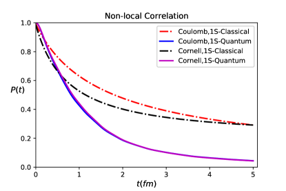
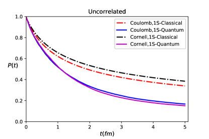
Figure 4: (color online) Comparison of $P(t)$ between the classical (black dot dashed for Cornell and red dot dashed for Coulomb) and quantum (pink solid for Cornell and blue solid for Coulomb) approach for the case of gluo-dissociation (left panel) and decoherence (right panel). The classical results at early time differ substantially for the two initial wavefunctions we used, whereas the quantum results are closer.

4.2 Results

The survival probability at any given time $t$ is defined as

$$P(t)=\langle\langle\ |\braket{\psi_{0}}{\psi_{\theta}(t)}|^{2}\ \rangle\rangle,$$ (65)

$\psi_{0}$ is the wavefunction in vacuum. The quantity $P(t)$ at freezeout is related to the observed suppression $R_{AA}$ of quarkonium states.

We modelled the background system evolution as a Bjorken expanding medium. The calculation was performed for $\Upsilon(1S)$ states. For the initial state, we considered two commonly studied forms. We chose the initial state as the eigenstate for a phenomenological vacuum Cornell potential and for comparison also considered the eigenstate of the Coulomb potential. (See Ref. Sharma:2019xum for details of the chosen parameters and comparisons of the wavefunction forms.)

We compare the results obtained using the stochastic Schorödinger equation (“quantum” evolution) to the results obtained by solving the rate equation (Eq. 2) which are labelled as “classical” evolution as it does not carry information about the coherent evolution of the wavefunction.

We have presented our comparison of survival probability $P(t)$ between the classical and quantum approach in Fig. 4 for decoherence (left panel) and gluo-dissociation (right panel).

The main conclusions are the following. First, we note that the rate equations give a larger survival probability than the quantum calculation even though the correlation of the noise term in the quantum calculation, and $\Gamma$ in the classical calculation are both given by chromo-electric field correlator. As mentioned above, this difference is because the quantum evolution tracks how the $Q\bar{Q}$ wavefunction evolves with time while in the classical case we use the initial wavefunction. Second, we note that experimental results for $\Upsilon(1S)$ (Refs. Chatrchyan:2011pe ; Khachatryan:2016xxp ; Sirunyan:2017lzi suggest $R_{AA}\sim 0.5$ for $1S$ states) which is substantially larger than the results for both correlated (gluo-dissociation) and the uncorrelated noise (decoherence) although the results for decoherence are closer to the experimental value (Fig. 4). However, there are additional effects one needs to consider before a quantitative comparison with the phenomenology can be made. For example, it was demonstrated in Ref. Miura:2019ssi that in the Abelian theory that inclusion of quantum dissipation can lead to an increase in $R_{AA}$ compared to the result for decoherence. Additionally, one needs to include feed-down contributions from excited states and take a realistic medium evolution model. Third, we note that the results do not depend strongly on the choice of the initial state (Cornell and Coulomb eigenstates) since these are narrow states. However, a similar calculation for $2S$ states shows a significant difference between the two. This implies that more effort needs to be made to understand the choice of the initial state. Finally, we note that for the quantum calculation with the parameters used, gluo-dissociation is a stronger effect. This shows that if the hierarchy between $m_{D}$ and $E_{b}$ is not very strong, a formalism to handle both effects is important.

While improvements along the suggested lines above are ongoing, the calculation makes it clear that quantum effects play an important role in the evolution of ${Q\bar{Q}}$ states.

5 Conclusions

The ${Q\bar{Q}}$ system in a static thermal medium is characterized by various energy scales, $M$, $1/r$, $E_{b}$, which need to be compared with the thermal scales $m_{D}$ and $T$. Since $M$ is much larger than the other scales, the system is amenable to treatments using non-relativistic EFTs.

If $1/r\gg E_{b},T$ the EFT of the system is potential NRQCD. The potentials in this theory are complex, reflecting the fact that the system can exchange energy and momentum with the environment. pNRQCD (Sec. 2.1) gives a useful framework to connect the coefficients to the decay rates.

One can calculate decay rates and relate them to the observed $R_{AA}$ in heavy ion collisions. These decay rates have been calculated to leading order using perturbation theory and using EFTs and applied to quarkonium phenomenology (Sec. 3).

Given that the coupling $g$ is strong at these scales, non-perturbative corrections are likely to be important. Over the last several years, significant progress has occurred in the calculation of these coefficients using lattice QCD.

In a medium evolving in time, there is an additional scale associated with the time scale of change of the background medium. If this time scale is comparable to the system scale ($1/E_{b}$), it becomes necessary to follow the coherent evolution of the system while taking into account decoherence due to the interactions with the environment. A natural framework for this is the theory of open quantum systems. The state of the system is described by a density matrix whose evolution equation can be obtained by integrating out the environment.

Over the last few years, master equations for the density matrices have been derived for quarkonia in the weak coupling limit. Similar equations can also be obtained under various hierarchies of the energy scales directly from pNRQCD. (See Sec. 4)

Combined with the progress in the non-perturbative calculation of the complex potentials and the chromo-electric correlator, these developments have brought the goal of the calculation of the observed yields of quarkonia in $AA$ collisions from first principles closer to fruition.

6 Acknowledgements

We acknowledge collaborators on various projects related to heavy quark and quarkonium physics, Samuel Aronson, Evan Borras, Sourendu Gupta, Brian Odegard, Anurag Tiwari, Ivan Vitev, and Ben-Wei Zhang. We also thank Dibyendu Bala, Saumen Datta for several illuminating discussions. We also acknowledge discussions and exchanges with Yukiano Akamatsu, Jean-Paul Blaizot, Nora Brambilla, Alexander Rothkopf, and Peter Petreczky.

7 Author contribution statement

This single author of this review is Rishi Sharma.

References

- (1) P. Romatschke, Int. J. Mod. Phys. E 19 (2010), 1-53 doi:10.1142/S0218301310014613 [arXiv:0902.3663 [hep-ph]].
- (2) D. A. Teaney, doi:10.1142/9789814293297_0004 [arXiv:0905.2433 [nucl-th]].
- (3) T. Hirano, Prog. Theor. Phys. Suppl. 195 (2012), 1-18 doi:10.1143/PTPS.195.1
- (4) H. Song, Pramana 84, 703-715 (2015) doi:10.1007/s12043-015-0971-2 [arXiv:1401.0079 [nucl-th]].
- (5) C. Gale, S. Jeon and B. Schenke, Int. J. Mod. Phys. A 28, 1340011 (2013) doi:10.1142/S0217751X13400113 [arXiv:1301.5893 [nucl-th]].
- (6) U. Heinz and R. Snellings, Ann. Rev. Nucl. Part. Sci. 63, 123-151 (2013) doi:10.1146/annurev-nucl-102212-170540 [arXiv:1301.2826 [nucl-th]].
- (7) C. Shen, Z. Qiu, H. Song, J. Bernhard, S. Bass and U. Heinz, Comput. Phys. Commun. 199, 61 (2016) doi:10.1016/j.cpc.2015.08.039 [arXiv:1409.8164 [nucl-th]].
- (8) S. Jeon and U. Heinz, Int. J. Mod. Phys. E 24, no.10, 1530010 (2015) doi:10.1142/S0218301315300106 [arXiv:1503.03931 [hep-ph]].
- (9) A. Jaiswal and V. Roy, Adv. High Energy Phys. 2016, 9623034 (2016) doi:10.1155/2016/9623034 [arXiv:1605.08694 [nucl-th]].
- (10) P. Romatschke and U. Romatschke, Phys. Rev. Lett. 99, 172301 (2007) doi:10.1103/PhysRevLett.99.172301 [arXiv:0706.1522 [nucl-th]].
- (11) U. W. Heinz, J. S. Moreland and H. Song, Phys. Rev. C 80, 061901 (2009) doi:10.1103/PhysRevC.80.061901 [arXiv:0908.2617 [nucl-th]].
- (12) B. Schenke, S. Jeon and C. Gale, Phys. Rev. C 82, 014903 (2010) doi:10.1103/PhysRevC.82.014903 [arXiv:1004.1408 [hep-ph]].
- (13) U. A. Wiedemann, Nucl. Phys. B 582, 409-450 (2000) doi:10.1016/S0550-3213(00)00286-8 [arXiv:hep-ph/0003021 [hep-ph]].
- (14) S. Caron-Huot, Phys. Rev. D 79, 065039 (2009) doi:10.1103/PhysRevD.79.065039 [arXiv:0811.1603 [hep-ph]].
- (15) A. Majumder, Phys. Rev. C 87, 034905 (2013) doi:10.1103/PhysRevC.87.034905 [arXiv:1202.5295 [nucl-th]].
- (16) E. Eichten, S. Godfrey, H. Mahlke and J. L. Rosner, Rev. Mod. Phys. 80 (2008) 1161 doi:10.1103/RevModPhys.80.1161 [hep-ph/0701208].
- (17) G. T. Bodwin, E. Braaten and G. P. Lepage, Phys. Rev. D 51, 1125 (1995) [Erratum-ibid. D 55, 5853 (1997)].
- (18) C. Quigg and J. L. Rosner, Phys. Rept. 56 (1979) 167. doi:10.1016/0370-1573(79)90095-4
- (19) E. Eichten, K. Gottfried, T. Kinoshita, K. D. Lane and T. M. Yan, Phys. Rev. D 21, 203 (1980) doi:10.1103/PhysRevD.21.203
- (20) S. W. Otto and J. D. Stack, Phys. Rev. Lett. 52 (1984) 2328. doi:10.1103/PhysRevLett.52.2328
- (21) M. B. Voloshin, Prog. Part. Nucl. Phys. 61 (2008), 455-511 doi:10.1016/j.ppnp.2008.02.001 [arXiv:0711.4556 [hep-ph]].
- (22) N. Brambilla et al., Eur. Phys. J. C 71 (2011) 1534 doi:10.1140/epjc/s10052-010-1534-9 [arXiv:1010.5827 [hep-ph]].
- (23) N. Brambilla, A. Pineda, J. Soto and A. Vairo, Nucl. Phys. B 566 (2000) 275 doi:10.1016/S0550-3213(99)00693-8 [hep-ph/9907240].
- (24) N. Brambilla, A. Pineda, J. Soto and A. Vairo, Rev. Mod. Phys. 77 (2005) 1423 doi:10.1103/RevModPhys.77.1423 [hep-ph/0410047].
- (25) N. Brambilla, A. Vairo, X. Garcia Tormo, i and J. Soto, Phys. Rev. D 80 (2009), 034016 doi:10.1103/PhysRevD.80.034016 [arXiv:0906.1390 [hep-ph]].
- (26) N. Brambilla, A. Pineda, J. Soto and A. Vairo, Phys. Lett. B 470 (1999), 215 doi:10.1016/S0370-2693(99)01301-5 [arXiv:hep-ph/9910238 [hep-ph]].
- (27) B. A. Kniehl, A. A. Penin, V. A. Smirnov and M. Steinhauser, Nucl. Phys. B 635 (2002), 357-383 doi:10.1016/S0550-3213(02)00403-0 [arXiv:hep-ph/0203166 [hep-ph]].
- (28) S. F. Radford and W. W. Repko, Phys. Rev. D 75, 074031 (2007) doi:10.1103/PhysRevD.75.074031 [arXiv:hep-ph/0701117 [hep-ph]].
- (29) W. W. Repko, M. D. Santia and S. F. Radford, Nucl. Phys. A 924 (2014), 65-73 doi:10.1016/j.nuclphysa.2014.01.005 [arXiv:1211.6373 [hep-ph]].
- (30) N. Brambilla, H. S. Chung, D. Müller and A. Vairo, JHEP 04 (2020), 095 doi:10.1007/JHEP04(2020)095 [arXiv:2002.07462 [hep-ph]].
- (31) C. Patrignani, T. K. Pedlar and J. L. Rosner, Ann. Rev. Nucl. Part. Sci. 63, 21-44 (2013) doi:10.1146/annurev-nucl-102212-170609 [arXiv:1212.6552 [hep-ex]].
- (32) Y. Burnier, O. Kaczmarek and A. Rothkopf, JHEP 12 (2015), 101 doi:10.1007/JHEP12(2015)101 [arXiv:1509.07366 [hep-ph]].
- (33) O. Kaczmarek, F. Karsch, P. Petreczky and F. Zantow, Phys. Lett. B 543 (2002) 41 doi:10.1016/S0370-2693(02)02415-2 [hep-lat/0207002].
- (34) S. Digal, S. Fortunato and P. Petreczky, Phys. Rev. D 68 (2003) 034008 doi:10.1103/PhysRevD.68.034008 [hep-lat/0304017].
- (35) O. Kaczmarek, S. Ejiri, F. Karsch, E. Laermann and F. Zantow, Prog. Theor. Phys. Suppl. 153 (2004) 287 doi:10.1143/PTPS.153.287 [hep-lat/0312015].
- (36) O. Kaczmarek and F. Zantow, Phys. Rev. D 71 (2005) 114510 doi:10.1103/PhysRevD.71.114510 [hep-lat/0503017].
- (37) M. Doring, K. Huebner, O. Kaczmarek and F. Karsch, Phys. Rev. D 75 (2007) 054504 doi:10.1103/PhysRevD.75.054504 [hep-lat/0702009].
- (38) S. Gupta, K. Huebner and O. Kaczmarek, Phys. Rev. D 77 (2008) 034503 doi:10.1103/PhysRevD.77.034503 [arXiv:0711.2251 [hep-lat]].
- (39) M. E. Peskin, Nucl. Phys. B 156, 365 (1979).
- (40) G. Bhanot and M. E. Peskin, Nucl. Phys. B 156 (1979) 391. doi:10.1016/0550-3213(79)90200-1
- (41) T. Matsui and H. Satz,, Physics Letters B, 178 (1986), 416-422.
- (42) F. Karsch, M. T. Mehr and H. Satz, Z. Phys. C 37, 617 (1988) doi:10.1007/BF01549722
- (43) F. Karsch and H. Satz, Zeitschrift für Physik C Particles and Fields, 51 2 (1991), 209.
- (44) S. Digal, P. Petreczky and H. Satz, Phys. Rev. D 64, 094015 (2001) doi:10.1103/PhysRevD.64.094015 [arXiv:hep-ph/0106017 [hep-ph]].
- (45) R. Rapp, D. Blaschke and P. Crochet, Prog. Part. Nucl. Phys. 65 (2010) 209 doi:10.1016/j.ppnp.2010.07.002 [arXiv:0807.2470 [hep-ph]].
- (46) R. Rapp and H. van Hees, [arXiv:0903.1096 [hep-ph]].
- (47) Z. Conesa del Valle et al., Nucl. Phys. Proc. Suppl. 214, 3 (2011).
- (48) M. Laine, O. Philipsen, P. Romatschke and M. Tassler, JHEP 0703 (2007) 054.
- (49) S. Datta, F. Karsch, P. Petreczky and I. Wetzorke, Phys. Rev. D 69 (2004) 094507 doi:10.1103/PhysRevD.69.094507 [hep-lat/0312037].
- (50) T. Umeda, K. Nomura and H. Matsufuru, Eur. Phys. J. C 39S1 (2005), 9-26 doi:10.1140/epjcd/s2004-01-002-1 [arXiv:hep-lat/0211003 [hep-lat]].
- (51) M. Asakawa and T. Hatsuda, Phys. Rev. Lett. 92 (2004), 012001 doi:10.1103/PhysRevLett.92.012001 [arXiv:hep-lat/0308034 [hep-lat]].
- (52) A. Jakovac, P. Petreczky, K. Petrov and A. Velytsky, Phys. Rev. D 75 (2007) 014506 doi:10.1103/PhysRevD.75.014506 [hep-lat/0611017].
- (53) A. Mocsy and P. Petreczky, Phys. Rev. D 77, 014501 (2008).
- (54) A. Mocsy and P. Petreczky, Phys. Rev. Lett. 99, 211602 (2007).
- (55) P. Petreczky, C. Miao and A. Mocsy, Nucl. Phys. A 855 (2011), 125-132 doi:10.1016/j.nuclphysa.2011.02.028 [arXiv:1012.4433 [hep-ph]].
- (56) A. Bazavov, P. Petreczky and A. Velytsky, doi:10.1142/9789814293297_0002 arXiv:0904.1748 [hep-ph].
- (57) G. Aarts, C. Allton, S. Kim, M. P. Lombardo, M. B. Oktay, S. M. Ryan, D. K. Sinclair and J. I. Skullerud, JHEP 1111 (2011) 103 doi:10.1007/JHEP11(2011)103 [arXiv:1109.4496 [hep-lat]].
- (58) F. Karsch, E. Laermann, S. Mukherjee and P. Petreczky, Phys. Rev. D 85 (2012) 114501 doi:10.1103/PhysRevD.85.114501 [arXiv:1203.3770 [hep-lat]].
- (59) P. Petreczky, J. Phys. G 39 (2012) 093002 doi:10.1088/0954-3899/39/9/093002 [arXiv:1203.5320 [hep-lat]].
- (60) S. Datta, Pramana 84, no. 5, 881 (2015) doi:10.1007/s12043-015-0975-y [arXiv:1403.8151 [nucl-th]].
- (61) A. Rothkopf, arXiv:1912.02253 [hep-ph].
- (62) S. Aronson, E. Borras, B. Odegard, R. Sharma and I. Vitev, Phys. Lett. B 778 (2018) 384 doi:10.1016/j.physletb.2018.01.038 [arXiv:1709.02372 [hep-ph]].
- (63) N. Borghini and C. Gombeaud, arXiv:1103.2945 [hep-ph].
- (64) N. Borghini and C. Gombeaud, Eur. Phys. J. C 72 (2012) 2000 doi:10.1140/epjc/s10052-012-2000-7 [arXiv:1109.4271 [nucl-th]].
- (65) C. Young and K. Dusling, Phys. Rev. C 87 (2013) no.6, 065206 doi:10.1103/PhysRevC.87.065206 [arXiv:1001.0935 [nucl-th]].
- (66) Y. Akamatsu and A. Rothkopf, Phys. Rev. D 85, 105011 (2012) doi:10.1103/PhysRevD.85.105011 [arXiv:1110.1203 [hep-ph]].
- (67) Y. Akamatsu, Phys. Rev. D 87 (2013) no.4, 045016 doi:10.1103/PhysRevD.87.045016 [arXiv:1209.5068 [hep-ph]].
- (68) Y. Akamatsu, Phys. Rev. D 91 (2015) no.5, 56002 doi:10.1103/PhysRevD.91.056002 [arXiv: [hep-ph/1403.5783]].
- (69) Y. Akamatsu, Phys. Rev. C 92 (2015) no.4, 044911 doi:10.1103/PhysRevC.92.044911 [arXiv:1503.08110 [nucl-th]].
- (70) S. Kajimoto, Y. Akamatsu, M. Asakawa and A. Rothkopf, arXiv:1705.03365 [nucl-th].
- (71) Y. Akamatsu, M. Asakawa, S. Kajimoto and A. Rothkopf, JHEP 1807 (2018) 029 doi:10.1007/JHEP07(2018)029 [arXiv:1805.00167 [nucl-th]].
- (72) T. Miura, Y. Akamatsu, M. Asakawa and A. Rothkopf, arXiv:1908.06293 [nucl-th].
- (73) Y. Akamatsu, [arXiv:2009.10559 [nucl-th]].
- (74) N. Brambilla, M. A. Escobedo, J. Soto and A. Vairo, Phys. Rev. D 96, no. 3, 034021 (2017) doi:10.1103/PhysRevD.96.034021 [arXiv:1612.07248 [hep-ph]].
- (75) N. Brambilla, M. A. Escobedo, J. Soto and A. Vairo, Phys. Rev. D 97 (2018) no.7, 074009 doi:10.1103/PhysRevD.97.074009 [arXiv:1711.04515 [hep-ph]].
- (76) N. Brambilla, M. A. Escobedo, A. Vairo and P. Vander Griend, Phys. Rev. D 100 (2019) no.5, 054025 doi:10.1103/PhysRevD.100.054025 [arXiv:1903.08063 [hep-ph]].
- (77) N. Brambilla et al. [TUMQCD Collaboration], arXiv:1912.00689 [hep-lat].
- (78) J. P. Blaizot, D. De Boni, P. Faccioli and G. Garberoglio, Nucl. Phys. A 946 (2016) 49 doi:10.1016/j.nuclphysa.2015.10.011 [arXiv:1503.03857 [nucl-th]].
- (79) J. P. Blaizot and M. A. Escobedo, JHEP 1806 (2018) 034 doi:10.1007/JHEP06(2018)034 [arXiv:1711.10812 [hep-ph]].
- (80) J. P. Blaizot and M. A. Escobedo, Phys. Rev. D 98 (2018) no.7, 074007 doi:10.1103/PhysRevD.98.074007 [arXiv:1803.07996 [hep-ph]].
- (81) X. Yao and B. Müller, Phys. Rev. C 97 (2018) no.1, 014908 Erratum: [Phys. Rev. C 97 (2018) no.4, 049903] doi:10.1103/PhysRevC.97.049903, 10.1103/PhysRevC.97.014908 [arXiv:1709.03529 [hep-ph]].
- (82) X. Yao and B. Müller, Phys. Rev. D 100 (2019) no.1, 014008 doi:10.1103/PhysRevD.100.014008 [arXiv:1811.09644 [hep-ph]].
- (83) X. Yao and T. Mehen, Phys. Rev. D 99 (2019) no.9, 096028 doi:10.1103/PhysRevD.99.096028 [arXiv:1811.07027 [hep-ph]].
- (84) X. Yao and B. Müller, Phys. Rev. D 97 (2018) no.7, 074003 doi:10.1103/PhysRevD.97.074003 [arXiv:1801.02652 [hep-ph]].
- (85) X. Yao and T. Mehen, [arXiv:2009.02408 [hep-ph]].
- (86) A. Islam and M. Strickland, [arXiv:2010.05457 [hep-ph]].
- (87) R. Sharma and A. Tiwari, Phys. Rev. D 101 (2020) no.7, 074004 doi:10.1103/PhysRevD.101.074004 [arXiv:1912.07036 [hep-ph]].
- (88) J. Casalderrey-Solana, H. Liu, D. Mateos, K. Rajagopal and U. A. Wiedemann, [arXiv:1101:0618]
- (89) A. Mocsy, P. Petreczky and M. Strickland, Int. J. Mod. Phys. A 28, 1340012 (2013) doi:10.1142/S0217751X13400125 [arXiv:1302.2180 [hep-ph]].
- (90) G. Aarts et al., Eur. Phys. J. A 53 (2017) no.5, 93 doi:10.1140/epja/i2017-12282-9 [arXiv:1612.08032 [nucl-th]].
- (91) A. Andronic et al., Eur. Phys. J. C 76, no. 3, 107 (2016) doi:10.1140/epjc/s10052-015-3819-5 [arXiv:1506.03981 [nucl-ex]].
- (92) O. Philipsen, Phys. Lett. B 535 (2002), 138-144 doi:10.1016/S0370-2693(02)01777-X [arXiv:hep-lat/0203018 [hep-lat]].
- (93) Y. Burnier, M. Laine and M. Vepsalainen, JHEP 01 (2008), 043 doi:10.1088/1126-6708/2008/01/043 [arXiv:0711.1743 [hep-ph]].
- (94) L. D. McLerran and B. Svetitsky, Phys. Rev. D 24 (1981) 450. doi:10.1103/PhysRevD.24.450
- (95) A. Beraudo, J.-P. Blaizot and C. Ratti, Nucl. Phys. A 806 (2008) 312 doi:10.1016/j.nuclphysa.2008.03.001 [arXiv:0712.4394 [nucl-th]].
- (96) J. I. Kapusta and C. Gale, doi:10.1017/CBO9780511535130
- (97) N. Brambilla, J. Ghiglieri, A. Vairo and P. Petreczky, Phys. Rev. D 78, 014017 (2008),
- (98) M. A. Escobedo and J. Soto, Phys. Rev. A 78 (2008) 032520 doi:10.1103/PhysRevA.78.032520 [arXiv:0804.0691 [hep-ph]].
- (99) N. Brambilla, M. A. Escobedo, J. Ghiglieri, J. Soto and A. Vairo, JHEP 1009 (2010) 038 doi:10.1007/JHEP09(2010)038 [arXiv:1007.4156 [hep-ph]].
- (100) M. A. Escobedo, J. Soto and M. Mannarelli, Phys. Rev. D 84, 016008 (2011) and references therein.
- (101) N. Brambilla, M. A. Escobedo, J. Ghiglieri and A. Vairo, JHEP 1112 (2011) 116 doi:10.1007/JHEP12(2011)116 [arXiv:1109.5826 [hep-ph]].
- (102) N. Brambilla, M. A. Escobedo, J. Ghiglieri and A. Vairo, JHEP 1107 (2011) 096 doi:10.1007/JHEP07(2011)096 [arXiv:1105.4807 [hep-ph]].
- (103) N. Brambilla, M. A. Escobedo, J. Ghiglieri and A. Vairo, JHEP 1305, 130 (2013) doi:10.1007/JHEP05(2013)130 [arXiv:1303.6097 [hep-ph]].
- (104) S. Biondini, N. Brambilla, M. A. Escobedo and A. Vairo, Phys. Rev. D 95 (2017) no.7, 074016 doi:10.1103/PhysRevD.95.074016 [arXiv:1701.06956 [hep-ph]].
- (105) D. Banerjee, S. Datta, R. Gavai and P. Majumdar, Phys. Rev. D 85 (2012) 014510 doi:10.1103/PhysRevD.85.014510 [arXiv:1109.5738 [hep-lat]].
- (106) H. T. Ding, A. Francis, O. Kaczmarek, F. Karsch, H. Satz and W. Soldner, J. Phys. G 38 (2011) 124070 doi:10.1088/0954-3899/38/12/124070 [arXiv:1107.0311 [nucl-th]].
- (107) A. Francis, O. Kaczmarek, M. Laine, T. Neuhaus and H. Ohno, Phys. Rev. D 92 (2015) no.11, 116003 doi:10.1103/PhysRevD.92.116003 [arXiv:1508.04543 [hep-lat]].
- (108) A. Rothkopf, T. Hatsuda and S. Sasaki, Phys. Rev. Lett. 108 (2012) 162001 doi:10.1103/PhysRevLett.108.162001 [arXiv:1108.1579 [hep-lat]].
- (109) Y. Burnier and A. Rothkopf, Phys. Rev. D 87 (2013) 114019 doi:10.1103/PhysRevD.87.114019 [arXiv:1304.4154 [hep-ph]].
- (110) Y. Burnier, O. Kaczmarek and A. Rothkopf, Phys. Rev. Lett. 114 (2015) no.8, 082001 doi:10.1103/PhysRevLett.114.082001 [arXiv:1410.2546 [hep-lat]].
- (111) Y. Burnier and A. Rothkopf, Phys. Rev. D 95 (2017) no.5, 054511 doi:10.1103/PhysRevD.95.054511 [arXiv:1607.04049 [hep-lat]].
- (112) D. Bala and S. Datta, arXiv:1909.10548 [hep-lat].
- (113) D. Bala and S. Datta, arXiv:1912.04826 [hep-lat].
- (114) N. Brambilla, J. Ghiglieri, P. Petreczky and A. Vairo, Phys. Rev. D 82 (2010) 074019 doi:10.1103/PhysRevD.82.074019 [arXiv:1007.5172 [hep-ph]].
- (115) M. Berwein, N. Brambilla, J. Ghiglieri and A. Vairo, JHEP 1303 (2013) 069 doi:10.1007/JHEP03(2013)069 [arXiv:1212.4413 [hep-th]].
- (116) M. Berwein, N. Brambilla and A. Vairo, Phys. Part. Nucl. 45 (2014) no.4, 656 doi:10.1134/S1063779614040029 [arXiv:1312.6651 [hep-th]].
- (117) M. Berwein, N. Brambilla, P. Petreczky and A. Vairo, Phys. Rev. D 93 (2016) no.3, 034010 doi:10.1103/PhysRevD.93.034010 [arXiv:1512.08443 [hep-ph]].
- (118) M. Berwein, N. Brambilla, P. Petreczky and A. Vairo, Phys. Rev. D 96 (2017) no.1, 014025 doi:10.1103/PhysRevD.96.014025 [arXiv:1704.07266 [hep-ph]].
- (119) A. Bazavov, N. Brambilla, H.-T. Ding, P. Petreczky, H.-P. Schadler, A. Vairo and J. H. Weber, Phys. Rev. D 93 (2016) no.11, 114502 doi:10.1103/PhysRevD.93.114502 [arXiv:1603.06637 [hep-lat]].
- (120) A. Bazavov et al. [TUMQCD Collaboration], Phys. Rev. D 98 (2018) no.5, 054511 doi:10.1103/PhysRevD.98.054511 [arXiv:1804.10600 [hep-lat]].
- (121) S. S. Adler et al. [PHENIX Collaboration], Phys. Rev. C 69 (2004) 014901 doi:10.1103/PhysRevC.69.014901 [nucl-ex/0305030].
- (122) A. Adare et al. [PHENIX Collaboration], Phys. Rev. Lett. 98 (2007) 232301 doi:10.1103/PhysRevLett.98.232301 [nucl-ex/0611020].
- (123) A. Adare et al. [PHENIX Collaboration], Phys. Rev. Lett. 101, 122301 (2008) doi:10.1103/PhysRevLett.101.122301 [arXiv:0801.0220 [nucl-ex]].
- (124) B. I. Abelev et al. [STAR Collaboration], Phys. Rev. C 80 (2009) 041902 doi:10.1103/PhysRevC.80.041902 [arXiv:0904.0439 [nucl-ex]].
- (125) A. Adare et al. [PHENIX Collaboration], Phys. Rev. C 84 (2011) 054912 doi:10.1103/PhysRevC.84.054912 [arXiv:1103.6269 [nucl-ex]].
- (126) L. Adamczyk et al. [STAR Collaboration], Phys. Rev. Lett. 111 (2013) no.5, 052301 doi:10.1103/PhysRevLett.111.052301 [arXiv:1212.3304 [nucl-ex]].
- (127) L. Adamczyk et al. [STAR Collaboration], Phys. Lett. B 722 (2013) 55 doi:10.1016/j.physletb.2013.04.010 [arXiv:1208.2736 [nucl-ex]].
- (128) A. Adare et al. [PHENIX Collaboration], Phys. Rev. C 86 (2012) 064901 doi:10.1103/PhysRevC.86.064901 [arXiv:1208.2251 [nucl-ex]].
- (129) L. Adamczyk et al. [STAR Collaboration], Phys. Rev. C 90 (2014) no.2, 024906 doi:10.1103/PhysRevC.90.024906 [arXiv:1310.3563 [nucl-ex]].
- (130) C. Aidala et al. [PHENIX Collaboration], Phys. Rev. C 90 (2014) no.6, 064908 doi:10.1103/PhysRevC.90.064908 [arXiv:1404.1873 [nucl-ex]].
- (131) A. Adare et al. [PHENIX Collaboration], Phys. Rev. C 93 (2016) no.3, 034903 doi:10.1103/PhysRevC.93.034903 [arXiv:1509.05380 [nucl-ex]].
- (132) L. Adamczyk et al. [STAR Collaboration], Phys. Lett. B 771 (2017) 13 doi:10.1016/j.physletb.2017.04.078 [arXiv:1607.07517 [hep-ex]].
- (133) J. Adam et al. [STAR Collaboration], Phys. Rev. Lett. 123 (2019) no.13, 132302 doi:10.1103/PhysRevLett.123.132302 [arXiv:1904.11658 [hep-ex]].
- (134) J. Adam et al. [STAR Collaboration], Phys. Lett. B 797 (2019) 134917 doi:10.1016/j.physletb.2019.134917 [arXiv:1905.13669 [nucl-ex]].
- (135) L. Adamczyk et al. [STAR Collaboration], Phys. Lett. B 735 (2014) 127 Erratum: [Phys. Lett. B 743 (2015) 537] doi:10.1016/j.physletb.2014.06.028, 10.1016/j.physletb.2015.01.046 [arXiv:1312.3675 [nucl-ex]].
- (136) L. Adamczyk et al. [STAR Collaboration], Phys. Rev. C 94 (2016) no.6, 064904 doi:10.1103/PhysRevC.94.064904 [arXiv:1608.06487 [nucl-ex]].
- (137) A. Adare et al. [PHENIX Collaboration], Phys. Rev. C 91 (2015) no.2, 024913 doi:10.1103/PhysRevC.91.024913 [arXiv:1404.2246 [nucl-ex]].
- (138) S. Chatrchyan et al. [CMS Collaboration], JHEP 1205, 063 (2012) doi:10.1007/JHEP05(2012)063 [arXiv:1201.5069 [nucl-ex]].
- (139) V. Khachatryan et al. [CMS Collaboration], Phys. Rev. Lett. 113, no. 26, 262301 (2014) doi:10.1103/PhysRevLett.113.262301 [arXiv:1410.1804 [nucl-ex]].
- (140) V. Khachatryan et al. [CMS Collaboration], Eur. Phys. J. C 77, no. 4, 252 (2017) doi:10.1140/epjc/s10052-017-4781-1 [arXiv:1610.00613 [nucl-ex]].
- (141) A. M. Sirunyan et al. [CMS Collaboration], Phys. Rev. Lett. 118, no. 16, 162301 (2017) doi:10.1103/PhysRevLett.118.162301 [arXiv:1611.01438 [nucl-ex]].
- (142) G. Aad et al. [ATLAS Collaboration], Phys. Lett. B 697 (2011) 294.
- (143) G. Aad et al. [ATLAS Collaboration], Phys. Lett. B 697, 294 (2011) doi:10.1016/j.physletb.2011.02.006 [arXiv:1012.5419 [hep-ex]].
- (144) M. Aaboud et al. [ATLAS Collaboration], Eur. Phys. J. C 78 (2018) no.9, 762 doi:10.1140/epjc/s10052-018-6219-9 [arXiv:1805.04077 [nucl-ex]].
- (145) M. Aaboud et al. [ATLAS Collaboration], Eur. Phys. J. C 78 (2018) no.9, 784 doi:10.1140/epjc/s10052-018-6243-9 [arXiv:1807.05198 [nucl-ex]].
- (146) B. Abelev et al. [ALICE Collaboration], [arXiv:1202.1383 [hep-ex]].
- (147) E. Abbas et al. [ALICE Collaboration], Phys. Rev. Lett. 111 (2013) 162301 doi:10.1103/PhysRevLett.111.162301 [arXiv:1303.5880 [nucl-ex]].
- (148) B. B. Abelev et al. [ALICE Collaboration], Phys. Lett. B 734, 314 (2014) doi:10.1016/j.physletb.2014.05.064 [arXiv:1311.0214 [nucl-ex]].
- (149) J. Adam et al. [ALICE Collaboration], JHEP 1507, 051 (2015) doi:10.1007/JHEP07(2015)051 [arXiv:1504.07151 [nucl-ex]].
- (150) J. Adam et al. [ALICE Collaboration], JHEP 1605 (2016) 179 doi:10.1007/JHEP05(2016)179 [arXiv:1506.08804 [nucl-ex]].
- (151) J. Adam et al. [ALICE Collaboration], Phys. Rev. Lett. 116 (2016) no.22, 222301 doi:10.1103/PhysRevLett.116.222301 [arXiv:1509.08802 [nucl-ex]].
- (152) J. Adam et al. [ALICE Collaboration], Phys. Lett. B 766 (2017) 212 doi:10.1016/j.physletb.2016.12.064 [arXiv:1606.08197 [nucl-ex]].
- (153) S. Acharya et al. [ALICE Collaboration], Phys. Rev. Lett. 119 (2017) no.24, 242301 doi:10.1103/PhysRevLett.119.242301 [arXiv:1709.05260 [nucl-ex]].
- (154) S. Acharya et al. [ALICE Collaboration], Phys. Lett. B 785 (2018) 419 doi:10.1016/j.physletb.2018.08.047 [arXiv:1805.04383 [nucl-ex]].
- (155) S. Acharya et al. [ALICE Collaboration], JHEP 1902 (2019) 012 doi:10.1007/JHEP02(2019)012 [arXiv:1811.12727 [nucl-ex]].
- (156) S. Acharya et al. [ALICE Collaboration], arXiv:1909.03158 [nucl-ex].
- (157) S. Acharya et al. [ALICE Collaboration], arXiv:1910.14404 [nucl-ex].
- (158) S. Chatrchyan et al. [CMS Collaboration], Phys. Rev. Lett. 107, 052302 (2011).
- (159) V. Khachatryan et al. [CMS Collaboration], Phys. Lett. B 770, 357 (2017) doi:10.1016/j.physletb.2017.04.031 [arXiv:1611.01510 [nucl-ex]].
- (160) A. M. Sirunyan et al. [CMS Collaboration], arXiv:1706.05984 [hep-ex].
- (161) A. Adare et al. [PHENIX Collaboration], Phys. Rev. C 77 (2008) 024912 Erratum: [Phys. Rev. C 79 (2009) 059901] doi:10.1103/PhysRevC.77.024912, 10.1103/PhysRevC.79.059901 [arXiv:0903.4845 [nucl-ex], arXiv:0711.3917 [nucl-ex]].
- (162) S. S. Adler et al. [PHENIX Collaboration], Phys. Rev. Lett. 96 (2006) 012304 doi:10.1103/PhysRevLett.96.012304 [nucl-ex/0507032].
- (163) A. Adare et al. [PHENIX Collaboration], Phys. Rev. Lett. 107 (2011) 142301 doi:10.1103/PhysRevLett.107.142301 [arXiv:1010.1246 [nucl-ex]].
- (164) L. Adamczyk et al. [STAR Collaboration], Phys. Rev. C 93 (2016) no.6, 064904 doi:10.1103/PhysRevC.93.064904 [arXiv:1602.02212 [nucl-ex]].
- (165) B. B. Abelev et al. [ALICE Collaboration], JHEP 1402, 073 (2014) doi:10.1007/JHEP02(2014)073 [arXiv:1308.6726 [nucl-ex]].
- (166) B. B. Abelev et al. [ALICE Collaboration], JHEP 1412, 073 (2014) doi:10.1007/JHEP12(2014)073 [arXiv:1405.3796 [nucl-ex]].
- (167) B. B. Abelev et al. [ALICE Collaboration], Phys. Lett. B 740, 105 (2015) doi:10.1016/j.physletb.2014.11.041 [arXiv:1410.2234 [nucl-ex]].
- (168) J. Adam et al. [ALICE Collaboration], JHEP 1506, 055 (2015) doi:10.1007/JHEP06(2015)055 [arXiv:1503.07179 [nucl-ex]].
- (169) J. Adam et al. [ALICE Collaboration], JHEP 1511, 127 (2015) doi:10.1007/JHEP11(2015)127 [arXiv:1506.08808 [nucl-ex]].
- (170) D. Adamová et al. [ALICE Collaboration], Phys. Lett. B 776 (2018) 91 doi:10.1016/j.physletb.2017.11.008 [arXiv:1704.00274 [nucl-ex]].
- (171) S. Acharya et al. [ALICE Collaboration], Eur. Phys. J. C 78 (2018) no.6, 466 doi:10.1140/epjc/s10052-018-5881-2 [arXiv:1802.00765 [nucl-ex]].
- (172) S. Acharya et al. [ALICE Collaboration], JHEP 1807 (2018) 160 doi:10.1007/JHEP07(2018)160 [arXiv:1805.04381 [nucl-ex]].
- (173) A. M. Sirunyan et al. [CMS Collaboration], Eur. Phys. J. C 77, no. 4, 269 (2017) doi:10.1140/epjc/s10052-017-4828-3 [arXiv:1702.01462 [nucl-ex]].
- (174) G. Aad et al. [ATLAS Collaboration], Phys. Rev. C 92 (2015) no.3, 034904 doi:10.1103/PhysRevC.92.034904 [arXiv:1505.08141 [hep-ex]].
- (175) The ATLAS collaboration, ATLAS-CONF-2015-050.
- (176) R. Aaij et al. [LHCb Collaboration], JHEP 1402, 072 (2014) doi:10.1007/JHEP02(2014)072 [arXiv:1308.6729 [nucl-ex]].
- (177) L. Grandchamp and R. Rapp, Phys. Lett. B 523 (2001) 60 doi:10.1016/S0370-2693(01)01311-9 [hep-ph/0103124].
- (178) L. Grandchamp and R. Rapp, Nucl. Phys. A 709 (2002) 415 doi:10.1016/S0375-9474(02)01027-8 [hep-ph/0205305].
- (179) L. Grandchamp, R. Rapp and G. E. Brown, Phys. Rev. Lett. 92 (2004) 212301 doi:10.1103/PhysRevLett.92.212301 [hep-ph/0306077].
- (180) L. Grandchamp, S. Lumpkins, D. Sun, H. van Hees and R. Rapp, Phys. Rev. C 73 (2006) 064906 doi:10.1103/PhysRevC.73.064906 [hep-ph/0507314].
- (181) M. Mannarelli and R. Rapp, Phys. Rev. C 72 (2005) 064905 doi:10.1103/PhysRevC.72.064905 [hep-ph/0505080].
- (182) D. Cabrera and R. Rapp, Phys. Rev. D 76 (2007) 114506 doi:10.1103/PhysRevD.76.114506 [hep-ph/0611134].
- (183) H. van Hees, M. Mannarelli, V. Greco and R. Rapp, Phys. Rev. Lett. 100 (2008) 192301 doi:10.1103/PhysRevLett.100.192301 [arXiv:0709.2884 [hep-ph]].
- (184) X. Zhao and R. Rapp, Phys. Lett. B 664 (2008) 253 doi:10.1016/j.physletb.2008.03.068 [arXiv:0712.2407 [hep-ph]].
- (185) X. Zhao and R. Rapp, [arXiv:0806.1239 [nucl-th]].
- (186) F. Riek and R. Rapp, Phys. Rev. C 82 (2010) 035201 doi:10.1103/PhysRevC.82.035201 [arXiv:1005.0769 [hep-ph]].
- (187) X. Zhao and R. Rapp, Phys. Rev. C 82 (2010) 064905 doi:10.1103/PhysRevC.82.064905 [arXiv:1008.5328 [hep-ph]].
- (188) A. Emerick, X. Zhao and R. Rapp, Eur. Phys. J. A 48 (2012) 72 doi:10.1140/epja/i2012-12072-y [arXiv:1111.6537 [hep-ph]].
- (189) X. Zhao, A. Emerick and R. Rapp, Nucl. Phys. A 904-905, 611c (2013) doi:10.1016/j.nuclphysa.2013.02.088 [arXiv:1210.6583 [hep-ph]].
- (190) S. Y. F. Liu and R. Rapp, Nucl. Phys. A 941 (2015) 179 doi:10.1016/j.nuclphysa.2015.07.001 [arXiv:1501.07892 [hep-ph]].
- (191) X. Du, R. Rapp and M. He, arXiv:1706.08670 [hep-ph].
- (192) S. Y. F. Liu and R. Rapp, Phys. Rev. C 97 (2018) no.3, 034918 doi:10.1103/PhysRevC.97.034918 [arXiv:1711.03282 [nucl-th]].
- (193) X. Du, S. Y. F. Liu and R. Rapp, Phys. Lett. B 796 (2019) 20 doi:10.1016/j.physletb.2019.07.032 [arXiv:1904.00113 [nucl-th]].
- (194) V. Greco, C. M. Ko and R. Rapp, Phys. Lett. B 595 (2004) 202 doi:10.1016/j.physletb.2004.06.064 [nucl-th/0312100].
- (195) B. Zhang, C. M. Ko, B. A. Li, Z. W. Lin and S. Pal, Phys. Rev. C 65 (2002) 054909 doi:10.1103/PhysRevC.65.054909 [nucl-th/0201038].
- (196) R. L. Thews, Nucl. Phys. A 783, 301 (2007) doi:10.1016/j.nuclphysa.2006.11.084 [hep-ph/0609121].
- (197) S. A. Bass, J. Phys. Conf. Ser. 50 279, (2006).
- (198) L. Yan, P. Zhuang and N. Xu, Phys. Rev. Lett. 97 (2006) 232301 doi:10.1103/PhysRevLett.97.232301 [nucl-th/0608010].
- (199) A. Capella, L. Bravina, E. G. Ferreiro, A. B. Kaidalov, K. Tywoniuk and E. Zabrodin, Eur. Phys. J. C 58 (2008) 437 doi:10.1140/epjc/s10052-008-0772-6 [arXiv:0712.4331 [hep-ph]].
- (200) L. Bravina, A. Capella, E. G. Ferreiro, A. B. Kaidalov, K. Tywoniuk and E. Zabrodin, Eur. Phys. J. C 61 (2009) 865 doi:10.1140/epjc/s10052-009-0906-5 [arXiv:0811.0790 [hep-ph]].
- (201) R. Peng and C. B. Yang, Nucl. Phys. A 837 (2010) 54. doi:10.1016/j.nuclphysa.2010.02.006
- (202) E. G. Ferreiro, Phys. Lett. B 731 (2014) 57 doi:10.1016/j.physletb.2014.02.011 [arXiv:1210.3209 [hep-ph]].
- (203) P. Braun-Munzinger and J. Stachel, Nucl. Phys. A 690 (2001) 119 doi:10.1016/S0375-9474(01)00936-8 [nucl-th/0012064].
- (204) R. L. Thews, M. Schroedter and J. Rafelski, Phys. Rev. C 63 (2001) 054905 doi:10.1103/PhysRevC.63.054905 [hep-ph/0007323].
- (205) Yan, L., Zhuang, P., and Xu, N. . Physical Review letters, 97 23,(2006) 232301.
- (206) A. P. Kostyuk, M. I. Gorenstein, H. Stoecker and W. Greiner, Phys. Rev. C 68 (2003) 041902 doi:10.1103/PhysRevC.68.041902 [hep-ph/0305277].
- (207) A. Andronic, P. Braun-Munzinger, K. Redlich and J. Stachel, J. Phys. G 38 (2011) 124081 doi:10.1088/0954-3899/38/12/124081 [arXiv:1106.6321 [nucl-th]].
- (208) S. Gupta and R. Sharma, Phys. Rev. C 89, no. 5, 057901 (2014) doi:10.1103/PhysRevC.89.057901 [arXiv:1401.2930 [nucl-th]].
- (209) J. Hoelck, F. Nendzig and G. Wolschin, Phys. Rev. C 95 (2017) no.2, 024905 doi:10.1103/PhysRevC.95.024905 [arXiv:1602.00019 [hep-ph]].
- (210) J. Hoelck and G. Wolschin, Eur. Phys. J. A 53 (2017) no.12, 241 doi:10.1140/epja/i2017-12441-0 [arXiv:1712.06871 [hep-ph]].
- (211) A. Dumitru, Y. Guo and M. Strickland, Phys. Lett. B 662 (2008) 37 doi:10.1016/j.physletb.2008.02.048 [arXiv:0711.4722 [hep-ph]].
- (212) A. Dumitru, Y. Guo, A. Mocsy and M. Strickland, Phys. Rev. D 79 (2009) 054019 doi:10.1103/PhysRevD.79.054019 [arXiv:0901.1998 [hep-ph]].
- (213) A. Dumitru, Y. Guo and M. Strickland, Phys. Rev. D 79 (2009) 114003 doi:10.1103/PhysRevD.79.114003 [arXiv:0903.4703 [hep-ph]].
- (214) M. Strickland, Phys. Rev. Lett. 107 (2011) 132301 doi:10.1103/PhysRevLett.107.132301 [arXiv:1106.2571 [hep-ph]].
- (215) M. Strickland and D. Bazow, Nucl. Phys. A 879 (2012) 25 doi:10.1016/j.nuclphysa.2012.02.003 [arXiv:1112.2761 [nucl-th]].
- (216) M. Margotta, K. McCarty, C. McGahan, M. Strickland and D. Yager-Elorriaga, Phys. Rev. D 83, 105019 (2011) [Erratum-ibid. D 84, 069902 (2011)].
- (217) C. S. Machado, F. S. Navarra, E. G. de Oliveira, J. Noronha and M. Strickland, Phys. Rev. D 88 (2013) 034009 doi:10.1103/PhysRevD.88.034009 [arXiv:1305.3308 [hep-ph]].
- (218) J. Alford and M. Strickland, Phys. Rev. D 88 (2013) 105017 doi:10.1103/PhysRevD.88.105017 [arXiv:1309.3003 [hep-ph]].
- (219) B. Krouppa, R. Ryblewski and M. Strickland, Phys. Rev. C 92 (2015) no.6, 061901 doi:10.1103/PhysRevC.92.061901 [arXiv:1507.03951 [hep-ph]].
- (220) B. Krouppa and M. Strickland, Universe 2 (2016) no.3, 16 doi:10.3390/universe2030016 [arXiv:1605.03561 [hep-ph]].
- (221) B. Krouppa, A. Rothkopf and M. Strickland, Phys. Rev. D 97 (2018) no.1, 016017 doi:10.1103/PhysRevD.97.016017 [arXiv:1710.02319 [hep-ph]].
- (222) P. P. Bhaduri, N. Borghini, A. Jaiswal and M. Strickland, Phys. Rev. C 100, no. 5, 051901 (2019) doi:10.1103/PhysRevC.100.051901 [arXiv:1809.06235 [hep-ph]].
- (223) J. Boyd, T. Cook, A. Islam and M. Strickland, Phys. Rev. D 100, no. 7, 076019 (2019) doi:10.1103/PhysRevD.100.076019 [arXiv:1905.05676 [hep-ph]].
- (224) T. Song and S. H. Lee, Phys. Rev. D 72 (2005) 034002 doi:10.1103/PhysRevD.72.034002 [hep-ph/0501252].
- (225) Y. Park, K. I. Kim, T. Song, S. H. Lee and C. Y. Wong, Phys. Rev. C 76 (2007) 044907 doi:10.1103/PhysRevC.76.044907 [arXiv:0704.3770 [hep-ph]].
- (226) T. Song, Y. Park, S. H. Lee and C. Y. Wong, Phys. Lett. B 659 (2008) 621 doi:10.1016/j.physletb.2007.11.084 [arXiv:0709.0794 [hep-ph]].
- (227) T. Song, W. Park and S. H. Lee, Phys. Rev. C 81 (2010) 034914 doi:10.1103/PhysRevC.81.034914 [arXiv:1002.1884 [nucl-th]].
- (228) T. Song, C. M. Ko, S. H. Lee and J. Xu, Phys. Rev. C 83 (2011) 014914 doi:10.1103/PhysRevC.83.014914 [arXiv:1008.2730 [hep-ph]].
- (229) T. Song, K. C. Han and C. M. Ko, Phys. Rev. C 84 (2011) 034907 doi:10.1103/PhysRevC.84.034907, 10.1103/PhysRevC.84.039902 [arXiv:1103.6197 [nucl-th]].
- (230) T. Song, K. C. Han and C. M. Ko, [arXiv:1109.6691 [nucl-th]]. Phys. Rev. C 85, 014902 (2012).
- (231) T. Song, C. M. Ko and S. H. Lee, Phys. Rev. C 87 (2013) no.3, 034910 doi:10.1103/PhysRevC.87.034910 [arXiv:1302.4395 [nucl-th]].
- (232) S. H. Lee, K. Morita, T. Song and C. M. Ko, Phys. Rev. D 89 (2014) no.9, 094015 doi:10.1103/PhysRevD.89.094015 [arXiv:1304.4092 [nucl-th]].
- (233) Y. Liu, C. M. Ko and T. Song, Phys. Rev. C 88 (2013) no.6, 064902 doi:10.1103/PhysRevC.88.064902 [arXiv:1307.4427 [hep-ph]].
- (234) T. Song, Phys. Rev. C 89, no. 4, 044903 (2014) doi:10.1103/PhysRevC.89.044903 [arXiv:1402.3451 [nucl-th]].
- (235) T. Song, C. M. Ko and S. H. Lee, Phys. Rev. C 91 (2015) no.4, 044909 doi:10.1103/PhysRevC.91.044909 [arXiv:1502.05734 [nucl-th]].
- (236) R. Baier and R. Rückl, Zeitschrift für Physik C Particles and Fields, 0170-9739, 19, 3, 251-266 (1983).
- (237) B. Humpert, Phys. Lett. B, 184, Issue 1, 105-107 (1987).
- (238) P. L. Cho and A. K. Leibovich, Phys. Rev. D 53, 6203 (1996).
- (239) P. L. Cho and A. K. Leibovich, Phys. Rev. D 53, 150 (1996).
- (240) E. Braaten, S. Fleming and A. K. Leibovich, Phys. Rev. D 63, 094006 (2001).
- (241) K. Sridhar, Phys. Rev. Lett. 77 (1996) 4880 doi:10.1103/PhysRevLett.77.4880 [hep-ph/9609285].
- (242) M. Butenschon and B. A. Kniehl, Phys. Rev. Lett. 106, 022003 (2011).
- (243) M. Butenschoen and B. A. Kniehl, Phys. Rev. D 84, 051501 (2011).
- (244) M. Butenschoen and B. A. Kniehl, Phys. Rev. Lett. 107, 232001 (2011).
- (245) K. Wang, Y. Q. Ma and K. T. Chao, Phys. Rev. D 85, 114003 (2012) doi:10.1103/PhysRevD.85.114003 [arXiv:1202.6012 [hep-ph]].
- (246) H. S. Shao, H. Han, Y. Q. Ma, C. Meng, Y. J. Zhang and K. T. Chao, JHEP 1505, 103 (2015) doi:10.1007/JHEP05(2015)103 [arXiv:1411.3300 [hep-ph]].
- (247) M. Gyulassy and X. N. Wang, Nucl. Phys. B 420 (1994) 583 doi:10.1016/0550-3213(94)90079-5 [nucl-th/9306003].
- (248) R. Baier, Y. L. Dokshitzer, A. H. Mueller, S. Peigne and D. Schiff, Nucl. Phys. B 484 (1997) 265 doi:10.1016/S0550-3213(96)00581-0 [hep-ph/9608322].
- (249) B. G. Zakharov, JETP Lett. 63 (1996) 952 doi:10.1134/1.567126 [hep-ph/9607440].
- (250) R. Baier, Y. L. Dokshitzer, A. H. Mueller and D. Schiff, Nucl. Phys. B 531 (1998) 403 doi:10.1016/S0550-3213(98)00546-X [hep-ph/9804212].
- (251) M. Gyulassy, P. Levai and I. Vitev, Nucl. Phys. B 571 (2000) 197 doi:10.1016/S0550-3213(99)00713-0 [hep-ph/9907461].
- (252) M. Gyulassy, P. Levai and I. Vitev, Nucl. Phys. B 594 (2001) 371 doi:10.1016/S0550-3213(00)00652-0 [nucl-th/0006010].
- (253) M. Gyulassy, P. Levai and I. Vitev, Phys. Rev. D 66 (2002) 014005 doi:10.1103/PhysRevD.66.014005 [nucl-th/0201078].
- (254) U. A. Wiedemann, Nucl. Phys. B 588 (2000) 303 doi:10.1016/S0550-3213(00)00457-0 [hep-ph/0005129].
- (255) C. A. Salgado and U. A. Wiedemann, Phys. Rev. D 68 (2003) 014008 doi:10.1103/PhysRevD.68.014008 [hep-ph/0302184].
- (256) A. Adil and I. Vitev, Phys. Lett. B 649, 139 (2007).
- (257) R. Sharma, I. Vitev and B. W. Zhang, Phys. Rev. C 80 (2009) 054902 doi:10.1103/PhysRevC.80.054902 [arXiv:0904.0032 [hep-ph]].
- (258) R. Sharma and I. Vitev, Phys. Rev. C 87 (2013) no.4, 044905 doi:10.1103/PhysRevC.87.044905 [arXiv:1203.0329 [hep-ph]].
- (259) Y. Makris and I. Vitev, JHEP 1910 (2019) 111 doi:10.1007/JHEP10(2019)111 [arXiv:1906.04186 [hep-ph]].
- (260) Y. Makris and I. Vitev, arXiv:1912.08008 [hep-ph].
- (261) N. Dutta and N. Borghini, Mod. Phys. Lett. A 30 (2015) no.37, 1550205 doi:10.1142/S0217732315502053 [arXiv:1206.2149 [nucl-th]].
- (262) H. P. Breuer and F. Petruccione, Oxford, UK: Univ. Pr. (2002) 625 p
- (263) G. Lindblad, Commun. Math. Phys. 48 (1976) 119. doi:10.1007/BF01608499
- (264) J. Casalderrey-Solana and D. Teaney, Phys. Rev. D 74 (2006) 085012 doi:10.1103/PhysRevD.74.085012 [hep-ph/0605199].