Quantum Control in Open and Periodically Driven Systems

Abstract

Quantum technology resorts to efficient utilization of quantum resources to realize technique innovation. The systems are controlled such that their states follow the desired manners to realize different quantum protocols. However, the decoherence caused by the system-environment interactions causes the states deviating from the desired manners. How to protect quantum resources under the coexistence of active control and passive decoherence is of significance. Recent studies have revealed that the decoherence is determined by the feature of the system-environment energy spectrum: Accompanying the formation of bound states in the energy spectrum, the decoherence can be suppressed. It supplies a guideline to control decoherence. Such idea can be generalized to systems under periodic driving. By virtue of manipulating Floquet bound states in the quasienergy spectrum, coherent control via periodic driving dubbed as Floquet engineering has become a versatile tool not only in controlling decoherence, but also in artificially synthesizing exotic topological phases. We will review the progress on quantum control in open and periodically driven systems. Special attention will be paid to the distinguished role played by the bound states and their controllability via periodic driving in suppressing decoherence and generating novel topological phases.

1 Introduction

Quantum technology is a class of technology that works by using quantum effects, such as quantum coherence, squeezing, and entanglement, to develop revolutionary techniques. Including quantum computation and algorithm [1, 2, 3, 4], quantum metrology and sensor [5, 6, 7, 8], quantum simulation [9], and quantum communication [10, 11], it opens an avenue to break through the technique limits for their classical counterparts from the principles of quantum mechanics. The main idea is to actively control the quantum states of relevant systems in the desired manners to realize different protocols. However, its realization is challenged by decoherence [12]. As a ubiquitous phenomenon in the microscopic world, decoherence is caused by the inevitable interaction of quantum systems with their environments. It makes the quantum resources degraded and the states deviating from the desired manners. Therefore, a thorough understanding of the detrimental influences of decoherence on quantum protocols and their efficient control are of importance in quantum technology. Many methods, such as entanglement concentration [13, 14], dynamical decoupling [15, 16], and feedback control [17, 18], have been proposed to suppress the effects of decoherence. Recent studies show that the structured environment, e.g. photonic crystal [19, 20, 21, 22] and localized surface plasmons [23, 24], dramatically changes or even inhibits the decoherence of quantum emitters [20, 25, 26]. Further studies reveal that these phenomena are due to the formation of a bound state in the energy spectrum of the total system [27]. It has been reported that such a bound state has profound impacts on many quantum protocols and nonequilibrium physics, e.g. entanglement preservation [28, 29, 30], noncanonical thermalization [31], quantum speed limit [32], and quantum metrology [33, 34, 35]. The results give us an insightful guideline to control decoherence via forming the bound state by quantum reservoir engineering [36, 37].

On the other hand, coherent control via periodic driving dubbed as Floquet engineering has become a versatile tool in quantum control [38]. The main idea resides in that the concepts of the energy spectrum and bound states of static systems can be completely inherited in the quasienergy spectrum of periodically driven systems according to Floquet theory. The bound-state mechanism in static systems was generalized to the periodically driven systems as the Floquet bound-state mechanism [39, 40, 41, 42]. Periodic driving largely extends the controllability of systems because time as a new control dimension is introduced. It overcomes the practical difficulty of reservoir engineering in static systems that the parameter is hard to change once the material is fabricated [43, 44, 45]. Engineering the quasienergy spectrum to form the Floquet bound states via periodic driving can also be applied to artificially synthesizing topological phases. The periodic driving induces an effective long-range hopping in lattice systems which is hard to experimentally realize in the static system [46, 47, 48, 49]. In this manner, widely tunable numbers of edge or surface states have been realized by periodic driving [50, 51, 47, 48, 49, 52, 53]. It is found that not only the topological phases hard to reach in the same setting of static systems but also many exotic topological phases totally absent in static systems can be realized by Floquet engineering [54, 50, 55].

We here review the progress on quantum control in open and periodically driven systems. The paper is organized as follows. In Sec. 2, the bound-state mechanism is given and the decoherence control based on the reservoir engineering is reviewed. The profound impacts of the bound state on entanglement preservation, quantum speedup, noncanonical thermalization, quantum metrology, and quantum plasmonics are explicitly analyzed. The Floquet engineering is reviewed in Sec. 3. The applications of Floquet engineering in decoherence control and the generation of exotic topological phases are explicitly discussed. Conclusion and outlook are made in Sec. 4.

2 Decoherence control in open quantum systems

Quantum technology is based on the efficient utilization of quantum resources, e.g. quantum coherence and entanglement, of the relevant systems to realize the technique innovation. However, any microscopic system is inevitably influenced by its surrounding environment and becomes an open system. It causes unwanted loss of quantum resources. Therefore, one of the important purposes of quantum control in open systems is to suppress decoherence. Depending on whether the open system has energy exchange with the environment, its decoherence can be classified into dissipation and dephasing. We focus on dissipation.

Open system influenced by its environment has a wide physical relevance in different experimental platforms of quantum technology. There are two types of open systems: Discrete- and continuous-variable systems. The discrete-variable system is generally a two-level system, which may be a two-level atom interacting with the radiation electromagnetic field [56], an electron spin in a quantum dot interacting with the nuclear spin [57, 58], or a superconducting charge qubit exposed to the charge noise [59]. The continuous-variable one may be a harmonic oscillator or a single-mode quantized optical field. The microscopic description of dissipation is based on the “system” + “reservoir” approach pioneered by Senitzky [60, 61]. The Hamiltonian is ($\hbar=1$)

$$\hat{H}=\omega_{0}\hat{o}^{\dagger}\hat{o}+\sum_{k}g_{k}(\hat{o}^{\dagger}\hat{a}_{k}+\hat{a}^{\dagger}_{k}\hat{o})+\sum_{k}\omega_{k}\hat{a}^{\dagger}_{k}\hat{a}_{k},$$ (1)

where $\hat{o}$ and $\hat{a}_{k}$ are the annihilation operator of the system with frequency $\omega_{0}$ and the $k$-th environmental mode with frequency $\omega_{k}$, and $g_{k}$ is the coupling strength. The coupling can be further characterized by the spectral density $J(\omega)=\sum_{k}|g_{k}|^{2}\delta(\omega-\omega_{k})$ [62]. The operator $\hat{o}=\hat{\sigma}_{-}$ with $\hat{\sigma}_{-}=|g\rangle\langle e|$ is the transition operator between the two levels for the discrete-variable system, $\hat{o}=\hat{b}$ is the annihilation operator for the bosonic continuous-variable system. One can check that the total excitation number $\hat{N}=\hat{\sigma}_{+}\hat{\sigma}_{-}+\sum_{k}\hat{a}^{\dagger}_{k}\hat{a}_{k}$ for both of the systems is conserved. Thus, the Hilbert space is split into the subspaces with a definite excitation number $N$.

The dynamics of the open system is obtainable by tracing out the environmental degrees of freedom from $\rho_{\text{T}}(t)$ satisfying the Liouville equation $\dot{\rho}_{\text{T}}(t)=-i[\hat{H},\rho_{\text{T}}(t)]$. However, it is difficult to be exactly done. A widely used reduction is the Markovian approximation [63, 64, 65], which works under the conditions that the system-environment coupling is weak and the environmental correlation time is much smaller than the one of the systems. Many systems, such as quantum dot [57, 58] and superconducting qubit [66], have shown the conditions where this approximation is inapplicable. It inspires particular attention to the non-Markovian dynamics [67, 62].

Supposing that the coupling is turned on at the initial time, we have $\rho_{\text{T}}(0)=\rho(0)\otimes\rho_{\text{E}}$, where $\rho(0)$ and $\rho_{\text{E}}$ are the initial state of system and environment, respectively. We consider that the environment is initially in a vacuum state. The dynamics governed by Eq. (1) in this case for the discrete-variable system is exactly solvable because only the Hilbert subspaces with $N=0$ and $1$ are involved [28]. The exact dynamics for the continuous-variable system is obtainable by the Feynman-Vernon influence functional theory [68] in the coherent-state representation [69]. After tracing out the environmental degrees of freedom, we obtain the non-Markovian master equation for both of the systems as

$$\dot{\rho}(t)=-i\omega(t)[\hat{o}^{\dagger}\hat{o},\rho(t)]+{\gamma(t)\over 2}[2\hat{o}\rho(t)\hat{o}^{\dagger}-\{\hat{o}^{\dagger}\hat{o},\rho(t)\}],$$ (2)

where $\gamma(t)-i\omega(t)=\dot{u}(t)/u(t)$ with $u(t)$ satisfying

$$\dot{u}(t)+i\omega_{0}u(t)+\int_{0}^{t}f(t-\tau)u(\tau)d\tau=0,$$ (3)

under $u(0)=1$. Here the kernel function is $f(t-\tau)=\int_{0}^{\infty}J(\omega)e^{-i\omega(t-\tau)}d\omega$.

A Laplace transform can linearize Eq. (3) into $\tilde{u}(z)=[z+i\omega_{0}+\int_{0}^{\infty}{J(\omega)\over z+i\omega}d\omega]^{-1}$. The solution of $u(t)$ is obtained by the inverse Laplace transform of $\tilde{u}(z)$, which can be done by finding its pole from

$$y(E)\equiv\omega_{0}-\int_{0}^{\infty}{J(\omega)\over\omega-E}d\omega=E,~{}(E=iz).$$ (4)

Note that the roots $E$ of Eq. (4) is just the eigenenergies of the total system (1) in the single-excitation space. Specifically, expanding the eigenstate as $|\Psi\rangle=(x\hat{o}^{\dagger}+\sum_{k}y_{k}\hat{b}_{k}^{\dagger})|0,\{0_{k}\}\rangle$ and substituting it into $\hat{H}|\Psi\rangle=E|\Psi\rangle$ with $E$ being the eigenenergy, we have $(E-\omega_{0})x=\sum_{k}g_{k}y_{k}$ and $y_{k}=g_{k}x/(E-\omega_{k})$. They readily lead to Eq. (4). Since $y(E)$ is a decreasing function in the regime $E<0$, Eq. (4) has one isolated root $E_{b}$ in this regime provided $y(0)<0$. While $y(E)$ is ill defined when $E>0$, Eq. (4) has infinite roots in this regime forming a continuous energy band. We call the eigenstate of the isolated eigenenergy $E_{b}$ bound state [28, 34]. After the inverse Laplace transform, we obtain

$$u(t)=Ze^{-iE_{b}t}+\int_{0}^{\infty}\frac{J(E)e^{-iEt}dE}{[E-\omega_{0}-\Delta(E)]^{2}+[\pi J(E)]^{2}},$$ (5)

where $\Delta(E)=\mathcal{P}\int_{0}^{\infty}\frac{J(\omega)}{E-\omega}d\omega$ with $\mathcal{P}$ being the Cauchy principal value. The first term with $Z=[1+\int_{0}^{\infty}{J(\omega)d\omega\over(E_{b}-\omega)^{2}}]^{-1}$ is from the bound state, and the second one is from the band energies. Oscillating with time in continuously changing frequencies, the integral tends to zero in the long-time condition due to out-of-phase interference. Thus, if the bound state is absent, then $\lim_{t\rightarrow\infty}u(t)=0$ characterizes a complete dissipation, while if the bound state is formed, then $\lim_{t\rightarrow\infty}u(t)=Ze^{-iE_{b}t}$ implies a dissipation suppression. A widely used type of spectral density reads $J(\omega)=\eta\omega^{s}\omega_{c}^{1-s}e^{-\omega/\omega_{c}}$, where $\eta$ is a dimensionless coupling constant, $\omega_{c}$ is a cutoff frequency, and $s$ is the Ohmicity parameter. Depending on the value of $s$, the environments are classified into a sub-Ohmic one ($0<s<1$), an Ohmic one ($s=1$), and a super-Ohmic one ($s>1$) [70]. We can check that the bound state is formed for the Ohmic-family spectral density when $\omega_{0}<\eta\omega_{c}\underline{\Gamma}(s)$, where $\underline{\Gamma}(s)$ is the Euler’s gamma function.

From the above analysis, we see that the non-Markovian dissipation dynamics for both of the discrete- and continuous-variable systems intrinsically depends on the character of the energy spectrum of the total system. In the following, we review the profound impact of the bound state on the different nonequilibrium physics of the systems.

2.1 Entanglement preservation

Quantum entanglement describes the nonclassical correlations between quantum subsystems, which was first recognized by Einstein, Podolsky, and Rosen [71]. It is an important resource to implement quantum protocols [72], e.g. quantum communication [73, 74, 75, 10, 11], quantum computation [1, 2, 3], and quantum metrology [5, 6, 7, 8]. However, it is generally degraded by the ubiquitous decoherence in the microscopic world. It was found that, quite different from the asymptotically decaying to zero of quantum coherence of a single two-level system, the entanglement of a bipartite two-level system influenced by two independent Markovian dissipative environments abruptly disappears in a finite time duration [76, 77, 78]. It is called entanglement sudden death. Further studies revealed that the dead entanglement can partially revive due to the non-Markovian effect [79, 80, 81]. Such finite extension of the entangled time is obviously not enough for quantum protocols and one generally desires to preserve the entanglement in the long-time limit. Indeed, it was shown that some entanglement can be preserved in the steady state by engineering a photonic crystal structured environment [82]. Actually, as demonstrated in the following, the entanglement preservation is a universal consequence of the existence of the system-environment bound state and the non-Markovian effect. The bound state provides the ability and the non-Markovian effect provides the dynamical way to preserve the entanglement [28, 83, 29].

Consider two independent two-level systems interacting with their respective dissipative environment. The dynamics of each two-level system is governed by Eq. (2) with $\hat{o}=\hat{\sigma}_{-}$ [83]. Solving the master equation under the initial condition $|\psi(0)\rangle=\frac{1}{\sqrt{2}}(|gg\rangle+|ee\rangle)$, we obtain

$$\rho(t)=\frac{1}{2}\big{\{}\big{[}|u(t)|^{2}|e\rangle\langle e|+(1-|u(t)|^{2})|g\rangle\langle g|\big{]}^{\otimes 2}+|g\rangle\langle g|^{\otimes 2}+[u(t)^{2}|e\rangle\langle g|^{\otimes 2}+\mathrm{H}.\mathrm{c}.]\big{\}}.$$ (6)

The entanglement of a bipartite two-level system is quantified by concurrence [84]. It is defined as $C(\rho)=\text{max}\{0,\lambda_{1}-\lambda_{2}-\lambda_{3}-\lambda_{4}\}$, where $\lambda_{i}$ is the $i$-th decreasing ordered eigenvalues of $R\equiv\sqrt{\sqrt{\rho}\tilde{\rho}\sqrt{\rho}}$ and $\tilde{\rho}$ is defined as $\tilde{\rho}\equiv(\hat{\sigma}_{y}\otimes\hat{\sigma}_{y})\rho^{*}(\hat{\sigma}_{y}\otimes\hat{\sigma}_{y})$ [85, 72]. Then we can obtain that the concurrence of Eq. (6) is $C(t)=\text{max}\{0,|u(t)|^{4}\}$. Combining with the knowledge that $u(t)$ is preserved when the bound state exists, we find that the formation of the bound state can also preserve the entanglement, which paves the way to stably protect entanglement from dissipation.

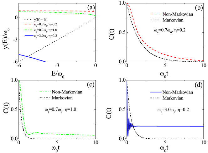
Figure 1: (a) Diagrammatic solution of Eq. (4) with different parameters of a super-Ohmic spectral density $s=3$. Entanglement evolution with parameters in the absence (b, c) and presence (d) of the bound state. Reproduced figures from [28].

Taking the super-Ohmic spectral density $J(\omega)=\eta\omega^{s}\omega_{0}^{1-s}e^{-\omega/\omega_{c}}$ with $s=3$, where the bound state is formed when $\omega_{0}-\eta\omega_{0}(\omega_{c}/\omega_{0})^{s}\underline{\Gamma}(s)<0$, as an example [28], Fig. 1(a) shows the diagrammatic solution of Eq. (4) for different parameter values. It reveals that as long as $\omega_{0}<2\eta\omega_{0}(\omega_{c}/\omega_{0})^{3}$, the bound state is formed. The corresponding entanglement dynamics are shown in Figs. 1(b), 1(c), and 1(d). Under the Markovian approximation, the concurrence always decays to zero irrespective of the existence of the bound state, whereas the exact non-Markovian dynamics reveals that the entanglement is preserved when the bound state is formed. The one-to-one correspondence between the formation of bound state and entanglement preservation clearly signifies the ability of the bound state in protecting the entanglement from decoherence.

Note that the entanglement preservation mechanism given above is also applicable to other spectral density [28] and other systems, e.g., nitrogen-vacancy centers embedded into the planar photonic-crystal cavities [30], continuous-variable system [86, 29], and quantum emitters coupled to the localized surface plasmons [26].

2.2 Quantum speed limit

The Heisenberg’s uncertainty principle sets a fundamental limit to measurement precision. One well-known example is that the precision of position is limited by the uncertainty of momentum as $\Delta x\geq\hbar/(2\Delta p)$. Such limitation also exists for the detection of time, which is known as the quantum speed limit (QSL) [87, 88, 89, 90]. It sets a bound on the minimal time a system needs to evolve between two distinguishable states [91, 92]. The QSL time for isolated systems is determined by the maximum of the Mandelstam-Tamn bound $\tau_{\text{ML}}=\pi\hbar/(2\Delta E)$ [88, 89] and Margolus-Levitin bound $\tau_{\text{ML}}=\pi\hbar/(2\bar{E})$ [92], where $\Delta E$ and $\bar{E}$ are the variation and the average of the Hamiltonian over the initial state, respectively. The QSL time for open systems characterizes the most efficient response of the system to the environmental influences. The Mandelstam-Tamm-type bound is generalized to open systems by using positive non-unitary maps [93, 94]. Based on a geometric approach, a unified bound including both Mandelstam-Tamm and Margolus-Levitin types has been formulated [95]. The QSL has attracted considerable attention because the efficient speedup of quantum systems plays remarkable roles in various areas of quantum physics, including nonequilibrium thermodynamics [96], quantum metrology [97], quantum optimal control [98], quantum computation [99], and quantum communication [100].

The previous studies revealed that the non-Markovian effect characterized by non-Markovianity can speed up the evolution of open systems [101, 102]. As a dynamical quantity, the non-Markovianity could not be seen as an essential reflection on the QSL of open systems. Furthermore, such attribution of the quantum speedup to the non-Markovianity is experimentally meaningless because the non-Markovianity is not an observable. Actually, it is the formation of the system-environment bound state that is the essential reason for the quantum speedup.

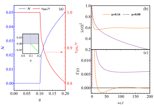
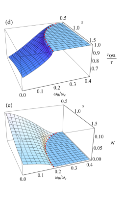
Figure 2: (a) Non-Markovianity $\mathcal{N}$ (blue dashed line) and QSL time $\tau_{\text{QSL}}$ (read solid line) for the Ohmic spectral density as a function of coupling constant $\eta$. The inset is the energy spectrum of the total system, where green dot-dashed line denotes the bound state. The obtained $|u(t)|^{2}$ (b) and the corresponding decay rate $\gamma(t)$ (c) with and without bound state. Parameters in (a), (b), and (c) are $\omega_{c}\tau=800$, $\omega_{0}/\omega_{c}=0.1$, and $s=1$, which determines that the bound state is formed when $\eta>0.1$. QSL time $\tau_{\text{QSL}}$ (d) and non-Markovianity $\mathcal{N}$ (e) as a function of the spectral power index $s$ and the system frequency $\omega_{0}$ for the spectral density $J(\omega)=\eta\omega^{s}\omega_{c}^{1-s}e^{-\omega/\omega_{c}}$. The red dashed line shows the critical values for forming the bound state. Parameters in (d) and (e) are $\omega_{c}\tau=800$ and $\eta=0.2$. Reproduced figures from [32].

To demonstrate this result, we consider again a dissipative two-level system [32]. Its dynamics follows the master equation (2) with $\hat{o}=\hat{\sigma}_{-}$. The QSL time between an initial state $\rho(0)=|\psi_{0}\rangle\langle\psi_{0}|$ and its target state $\rho(\tau)$ is defined as $\tau_{\text{QSL}}=\sin^{2}\mathcal{B}[\rho(0),\rho(\tau)]/\Lambda_{\tau}^{(\infty)}$ [101], where $\mathcal{B}[\rho(0),\rho(\tau)]\equiv\arccos\sqrt{\langle\psi_{0}|\rho(\tau)|\psi_{0}\rangle}$ is the Bures angle between $\rho(0)$ and $\rho(\tau)$, and $\Lambda_{\tau}^{(\infty)}=(1/\tau)\int_{0}^{\tau}dt||\dot{\rho}(t)||_{\infty}$ with $\|\hat{A}\|_{\infty}$ equaling to the largest eigenvalue of $\sqrt{\hat{A}^{\dagger}\hat{A}}$. From Eq. (2), the QSL time for this system

$$\tau_{\text{QSL}}=\frac{1-|u(\tau)|^{2}}{(1/\tau)\int_{0}^{\tau}|\partial_{t}|u(t)|^{2}|dt},$$ (7)

is achieved when $|\psi_{0}\rangle=|e\rangle$. In order to make a comparison with the previous works, we also calculate the non-Markovianity defined as $\mathcal{N}=\max_{\rho_{1,2}(0)}\int_{\sigma>0}dt\sigma(t,\rho_{1,2}(0))$, where $\sigma(t,\rho_{1,2}(0))=\dot{D}(\rho_{1}(t),\rho_{2}(t))$ is the change rate of the trace distance $D(\rho_{1}(t),\rho_{2}(t))=\frac{1}{2}\text{Tr}|\rho_{1}(t)-\rho_{2}(t)|$ between states $\rho_{1,2}(t)$ evolving from their respective initial forms $\rho_{1,2}(0)$ [103]. For the two-level system, it has been proven that the optimal pair of initial states to maximize $\mathcal{N}$ are $\rho_{1}(0)=|g\rangle\langle g|$ and $\rho_{2}(0)=|e\rangle\langle e|$ [101], which means $D(\rho_{1}(t),\rho_{2}(t))=|u(t)|^{2}$. Then one can readily verify $\mathcal{N}={1\over 2}\big{[}|u(\tau)|^{2}-1+\int_{0}^{\tau}|\partial_{t}|u(t)|^{2}|dt\big{]}$, which connects to $\tau_{\text{QSL}}$ as $\tau_{\text{QSL}}=\tau{1-|u(\tau)|^{2}\over 1-|u(\tau)|^{2}+2\mathcal{N}}$.

The numerical results for the Ohmic-family spectral density are shown in Fig. 2. From Fig. 2(a) one can find that both the non-Markovianity and quantum speedup show a perfect correspondence with the formation of bound state. In the absence of the bound state, there is no non-Makrovianity and quantum speedup. Whereas, an abrupt increase of the non-Markovianity and an abrupt decrease of the QSL time are observed when the bound state is formed. The corresponding excited-state population $\text{Tr}[\hat{\sigma}_{+}\hat{\sigma}_{-}\rho(t)]=|u(t)|^{2}$ and the decay rate $\gamma(t)$ are plotted in Figs. 2(b) and 2(c), respectively. We can see that $\gamma(t)$ in the absence of the bound state tends to a positive constant after a short-time jolt. Its complete positivity causes $|u(t)|^{2}$ to decay to zero monotonically. Since the system equilibrates in an asymptotic manner to its ground state, there is no more efficient evolution than the evolution characterized by $\tau$ and thus $\tau_{\text{QSL}}=\tau$. When the bound state is formed, the competition between the environmental backaction and the dissipation causes $\gamma(t)$ to transiently take a negative value and asymptotically approaches zero. Thus, after some short-time oscillations, $|u(t)|^{2}$ tends to a finite value. The transient increase of $|u(t)|^{2}$ causes the increase of the distinguishability and the decrease of $\tau_{\text{QSL}}$. The system here has a great capacity to speedup. Hence the bound state supplies a latent capability, while the non-Markovianity only supplies the dynamical way to the system for quantum speedup. The result is confirmed in the general cases with changing $\omega_{0}$ and $s$ in Figs. 2 (d) and 2(e).

The relationship between the bound state and quantum speedup reveals a mechanism for quantum speedup. It may be of both theoretical and experimental interests in exploring the ultimate QSL in realistic environments, and may open new perspectives for devising active quantum speedup devices.

2.3 Noncanonical thermalization

In statistical mechanics, systems in equilibrium with its weakly coupled environment are described by a canonical state at the same temperature as the environment. Being called canonical thermalization, this is based on the assumption of ergodicity. The assumption relies on the subjective lack of knowledge of systems. Therefore, how and when systems microscopically equilibrate from any initial state to a unique canonical state has attracted much attention [104, 105, 106, 107, 108, 109, 110, 111, 112, 113, 114, 115]. It was revealed that the assumption of ergodicity could be abandoned by examining the entanglement induced by the system-environment interaction, by which the canonical state can be achieved without referring to ensembles or time averages [104]. It inspires the studies of canonical thermalization from the dynamics of open quantum systems [116, 117, 118, 119, 120]. It is expected that equilibrium statistical physics should be an emergent steady-state limit of the nonequilibrium dynamics. It was shown that the canonical thermalization is valid only in the limit of the vanishing coupling and the memoryless correlation function of the environment [116, 118]. However, in real physical situations, e.g. photonic crystal [121] and semiconductor phonon [122] environments, low-dimensional solid-state system [123], and optical systems [124, 125], these conditions are generally invalid and the strong memory effect of the environment may even cause the anomalous decoherence behavior [126, 25, 26]. Therefore, to microscopically bridge between an arbitrary initial state of the open system and its equilibrium state via studying its equilibration dynamics is desired to check the validity regime of the assumption of ergodicity [31].

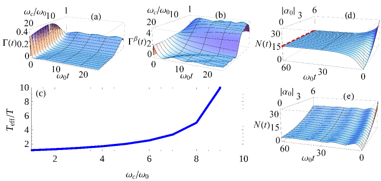
Figure 3: $\Gamma(t)$ (a) and $\Gamma^{\beta}(t)$ (b) in different $\omega_{c}$. (c) $T_{\text{eff}}$ evaluated when $t=100/\omega_{0}$. $\eta=0.1$, $\beta=0.1/\omega_{0}$, and $s=1$ have been used. Mean photon number $N(t)$ in different initial condition $\alpha_{0}$ when $\eta=0.05$ (d) and $0.2$ (e), where the red dashed line is obtained from Eq. (10). Reproduced figure from [31].

To address this issue, we consider a continuous-variable system described by a quantum harmonic oscillator interacting with a finite-temperature environment [31]. The Hamiltonian follows Eq. (1) with $\hat{o}=\hat{b}$. After generalizing Eq. (2) to the finite-temperature case, we obtain the exact non-Markovian master equation as

$$\begin{split}\dot{\rho}(t)=&-i\Omega(t)\big{[}\hat{b}^{\dagger}\hat{b},\rho(t)\big{]}+\Big{[}\Gamma(t)+\frac{\Gamma_{\beta}(t)}{2}\Big{]}\big{[}2\hat{b}\rho(t)\hat{b}^{\dagger}-\{\hat{b}^{\dagger}\hat{b},\rho(t)\}\big{]}\\ &+\frac{\Gamma_{\beta}(t)}{2}\big{[}2\hat{b}^{\dagger}\rho(t)\hat{b}-\{\hat{b}\hat{b}^{\dagger},\rho(t)\}\big{]},\end{split}$$ (8)

where $\Gamma(t)+i\Omega(t)=-\dot{u}(t)/u(t)$ and $\Gamma_{\beta}(t)=\dot{v}(t)+2v(t)\Gamma(t)$. The function $u(t)$ satisfies Eq. (3) and $v(t)=\int_{0}^{t}dt_{1}\int_{0}^{t}dt_{2}u^{*}(t_{1})\mu(t_{1}-t_{2})u(t_{2})$, where $\mu(x)=\int_{0}^{\infty}\bar{n}(\omega)J(\omega)e^{-i\omega x}d\omega$ with $\beta=(k_{B}T)^{-1}$ and $\bar{n}(\omega)=(e^{\beta\omega}-1)^{-1}$. According to the detailed balance condition, as long as $\Gamma(t)$ and $\Gamma^{\beta}(t)$ are positive, the steady state of Eq. (8) must be

$$\rho(\infty)=\sum_{n=0}^{\infty}\frac{[\Gamma^{\beta}(\infty)/(2\Gamma(\infty))]^{n}}{[1+\Gamma^{\beta}(\infty)/(2\Gamma(\infty))]^{n+1}}|n\rangle\langle n|,$$ (9)

which defines a unique canonical state irrespective of the initial state

$$\rho_{\text{con}}\equiv\rho(\infty)=e^{-\beta_{\text{eff}}\hat{H}_{\text{s}}}/\text{Tr}_{\text{s}}e^{-\beta_{\text{eff}}\hat{H}_{\text{s}}},~{}(\beta_{\text{eff}}=1/k_{B}T_{\text{eff}}),$$ (10)

with $T_{\text{eff}}=\frac{\omega_{0}}{k_{B}}\{\ln[1+\frac{2\Gamma(\infty)}{\Gamma^{\beta}(\infty)}]\}^{-1}$. The effective temperature $T_{\text{eff}}$ reduces to the environmental temperature $T$ in the Markovian limit. This can be verified from the Markovian solution of Eq. (3), i.e. $u_{\text{MA}}(t)=e^{-(\Gamma_{0}+i\Omega_{0})t}$ with $\Gamma_{0}=\pi J(\omega_{0})$ and $\Omega_{0}=\omega_{0}+\mathcal{P}\int{J(\omega)\over\omega_{0}-\omega}d\omega$, which leads to $\Gamma_{\text{MA}}(t)=\kappa$, $\Omega_{\text{MA}}(t)=\Omega_{0}$, and $\Gamma^{\beta}_{\text{MA}}(t)=2\kappa\bar{n}(\omega_{0})$. We readily have $T_{\text{eff,MA}}=T$. Thus, the canonical ensemble assumption in statistical mechanics can be dynamically confirmed under the Markovian approximation.

In the non-Markovian situation, the obtained $\Gamma(t)$, $\Gamma^{\beta}(t)$, and $T_{\text{eff}}$ for the Ohmic spectral density are plotted in Fig. 3. In the absence of the bound state when $\omega_{c}<10\omega_{0}$, both $\Gamma(t)$ and $\Gamma^{\beta}(t)$ tend to positive constant values asymptotically. Their positivity guarantees the validity of Eq. (9). Consequently, the system approaches a canonical state governed by Eq. (10), as shown in Fig. 3(c), irrespective of in what state the system initially resides. Here it is qualitatively consistent with the one under the Markovian approximation. However, whenever the bound state is formed in the regime $\omega_{c}\geq 10\omega_{0}$ of Fig. 3, $\Gamma(t)$ and $\Gamma^{\beta}(t)$ possess transient negative values and approach zero asymptotically. Their vanishing values cause the ill definition of the canonical state (10). In Fig. 3(c), we really see that $T_{\text{eff}}$ changes to be divergent when the parameters tend to the critical point forming the bound state. Another interesting observation is that even when the equilibration to a canonical state is valid in the absence of the bound state, $T_{\text{eff}}$ still shows a dramatically quantitative difference from $T$. Figure 3(d) indicates that the equilibrium state matching with Eq. (9) is independent of the initial condition when the bound state is absent. However, this is not true as long as the bound state is formed [see Fig. 3(e)]. This result confirms again the breakdown of canonical thermalization due to the formation of the bound state.

Building a unified framework to treat the issues in equilibrium and nonequilibrium statistical mechanics, the result gives a microscopic description of the canonical thermalization and reveals the working condition of the assumption of ergodicity as the basis of the equilibrium statistical mechanics.

2.4 Quantum metrology

Quantum metrology employs quantum resources, such as entanglement and squeezing, to attain a measurement precision surpassing the limit achievable in classical physics [5, 127, 128, 129, 130]. It has been found that the metrology precision with a $N$-body entangled state reaches the Heisenberg limit (HL) scaling $N^{-1}$, which is far better than the shot-noise limit (SNL) $N^{-1/2}$ revealed by $N$-body product state [5]. Such an enhancement inspires the application in gravitation wave detection [131, 132] and atomic clocks [133, 134]. The main obstacle of quantum metrology in practical applications is decoherence. It has been shown that the Markovian decoherence degrades the scaling from the HL back to the SNL [135, 8]. Some studies revealed that the non-Markovian effect can retrieve quantum superiority to beat the SNL [136, 137, 138]. However, it works only in the short encoding time condition. The precision gets worse in the long-time condition. Therefore, how to achieve metrology precision surpassing the SNL in the long encoding time condition in the presence of the dissipative environment is of significance in the practical application of quantum metrology.

2.4.1 Quantum metrology based on Mech-Zehnder interferometer

To estimate a frequency $\gamma$ of a system, we prepare two modes of optical fields with frequency $\omega_{0}$ and the initial state $|\Psi_{\text{in}}\rangle$ as the probe to input into the Mech-Zehnder interferometer (MZI). The input-output relation of the MZI reads $|\Psi_{\text{out}}\rangle=\hat{V}\hat{U}_{0}(\gamma,t)\hat{V}|\Psi_{\text{in}}\rangle$, where $\hat{V}=\exp[i\frac{\pi}{4}(\hat{b}_{1}^{\dagger}\hat{b}_{2}+\hat{b}_{2}^{\dagger}\hat{b}_{1})]$ is the action of $\text{BS}_{i}$ and $\hat{U}_{0}(\gamma,t)=\exp(-{i\hat{H}_{0}t/\hbar})$ with $\hat{H}_{0}=\hbar\omega_{0}\sum_{m=1,2}\hat{b}_{m}^{\dagger}\hat{b}_{m}+\hbar\gamma\hat{b}_{2}^{\dagger}\hat{b}_{2}$ describes the free evolution of the probe and its coupling to the system for encoding. The photon difference $\hat{M}=\hat{b}^{\dagger}_{1}\hat{b}_{1}-\hat{b}^{\dagger}_{2}\hat{b}_{2}$ is measured by $\text{D}_{i}$. If we use the squeezed state $|\Psi_{\text{in}}\rangle=\hat{D}_{\hat{b}_{1}}\hat{S}_{\hat{b}_{2}}|0,0\rangle$, where $\hat{D}_{\hat{b}}=e^{\alpha\hat{b}^{\dagger}-\alpha^{\ast}\hat{b}}$ with $\alpha=|\alpha|e^{i\varphi}$, $\hat{S}_{\hat{b}}=e^{\frac{1}{2}(\xi^{\ast}\hat{b}^{2}-\xi\hat{b}^{\dagger 2})}$ with $\xi=re^{i\phi}$, and $|0,0\rangle$ is the vacuum state, then we have the best precision of estimating $\gamma$ via $\delta\gamma=\frac{\delta M}{|\partial\bar{M}/\partial\gamma|}$ as [139]

$$\min\delta\gamma=\frac{[(1-\beta)e^{-2r}+\beta]^{1\over 2}}{t\sqrt{N}|1-2\beta|},~{}(\beta\equiv\sinh^{2}r/N)$$ (11)

when $\phi=2\varphi$ and $\gamma t={(2m+1)\pi/2}$ for $m\in\mathbb{Z}$. If the squeezing is absent, then $\min\delta\gamma|_{\beta=0}=(tN_{0}^{1/2})^{-1}$ with $N_{0}=|\alpha|^{2}$ is just the SNL. For $\beta\neq 0$, using $e^{-2r}\simeq 1/(4\sinh^{2}r)$ for $N\gg 1$ and optimizing $\beta$, we obtain $\min\delta\gamma|_{\beta=(2\sqrt{N})^{-1}}=(tN^{3/4})^{-1}$, which is called Zeno limit. It beats the SNL and manifests the superiority of the squeezing in metrology.

In practice, the above ideal encoding dynamics is obscured by the decoherence. The decoherence in MZI comes from the photon loss. Consider that the second optical field is affected by photon loss during the parameter encoding process, then its dynamics is governed by Eq. (2) with $\hat{o}=\hat{b}_{2}$. We can calculate [34]

$$\bar{M} = \text{Re}[u(t)e^{i\omega_{0}t}](\sinh^{2}r-|\alpha|^{2}),$$

$$\delta M^{2} = \text{Im}[u(t)e^{i\omega_{0}t}]^{2}[|\alpha\cosh r-\alpha^{\ast}\sinh re^{i\phi}|^{2}+\sinh^{2}r]$$ (12)

$$+\text{Re}[u(t)e^{i\omega_{0}t}]^{2}[|\alpha|^{2}+\frac{1}{2}\sinh^{2}(2r)]+\frac{1-|u(t)|^{2}}{2}N,$$

where $u(t)$ satisfies Eq. (3) with the replacement of $\omega_{0}$ by $\omega_{0}+\gamma$. Applying the Markovian solution $u_{\text{MA}}(t)=e^{-[\kappa+i(\omega_{0}+\gamma+\Delta)]t}$ with $\kappa=\pi J(\omega_{0}+\gamma)$ and $\Delta=\mathcal{P}\int_{0}^{\infty}{J(\omega)\over\omega_{0}+\gamma-\omega}d\omega$, we obtain $\min\delta\gamma\simeq({e^{2\kappa t}-1\over 2Nt^{2}})^{1/2}$ when $\beta=(2\sqrt{N})^{-1}$ and $\varphi=2\phi$. Getting divergent in the long-time limit, its minimum at $t=\kappa^{-1}$ returns the SNL $e\kappa(2N)^{-1/2}$. Thus, the quantum superiority of the scheme in the Markovian noise disappears completely, which is consistent with the result in the Ramsey spectroscopy [135].

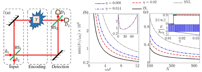
Figure 4: (a) Scheme of Mach-Zehnder interference. Metrology precision as a function of time $t$ (b) and total photon number (c) in different $\eta$ of the Ohmic spectral density. The inset of (c) shows steady-state value $Z=|c(\infty)|$ and the energy spectrum. Parameters are $\beta=(2\sqrt{N})^{-1}$, $\omega_{c}=300\omega_{0}$, $\gamma=\pi\omega_{0}$, $t=10\omega_{0}^{-1}$ for (c) and $N=100$ for (b). Reproduced figures from [34].

In the non-Markovian case, focusing on the situation in the presence of the bound state, we can obtain the precision using the long-time solution $Ze^{-iE_{b}t}$ of Eq. (5)

$$\min\delta\gamma|_{\beta=(2\sqrt{N})^{-1}}={(tN^{3/4})^{-1}\over Z}[1+{1-Z^{2}\over 2Z^{2}}N^{1\over 2}]^{1\over 2},$$ (13)

when $t={(2m+1)\pi\over 2|\omega_{0}-\varpi_{\text{b}}|}$ and $\varphi=2\phi$. It is interesting to see that, different from the previous results [135, 8, 136, 137, 138], where $\delta\gamma$ gets divergent with time, $\delta\gamma$ decreases with the encoding time monotonically. This is numerically confirmed by the results in Fig. 4(d). Thus, the bound state makes the superiority of the encoding time as a resource in the ideal metrology case retrieved. The relation of the precision with the total photon number in Fig. 4(c) reveals that, with the formation of the bound state, not only the SNL can be surpassed, but also the ideal Zeno limit is asymptotically retrieved with $Z$ approaching unit [see Eq. (13)].

2.4.2 Quantum metrology based on Ramsey spectroscopy

Another widely used metrology scheme is based on the atomic Ramsey spectroscopy [135]. To estimate atomic frequency $\omega_{0}$, we use $n$ two-level atoms prepared in $|\Psi_{\text{in}}\rangle=(|g\rangle^{\otimes n}+|e\rangle^{\otimes n})/\sqrt{2}$ as the probe. It freely evolves to $|\Psi_{\omega_{0}}\rangle=(|g\rangle^{\otimes n}+e^{-in\omega_{0}t}|e\rangle^{\otimes n})/\sqrt{2}$. After performing a CNOT gate with the first atom as the controller and the others as the target to disentangle them and a Hadamard gate on the first atom, the measuring of the excited-state population $\hat{M}=\hat{\sigma}_{+}\hat{\sigma}_{-}$ on the first atom results in $\bar{M}=\sin^{2}{n\omega_{0}t\over 2}$ and $\Delta M=|\sin{n\omega_{0}t}|/2$. Repeating the experiment in duration $T$, we have $N=T/t$ results. According to the central limit theorem, we have $\delta M=\sqrt{\Delta M\over N}$. Then the propagation of error leads to the best error in estimating $\omega_{0}$ as

$$\delta\omega_{0}|_{\text{ideal}}=(n^{2}Tt)^{-1/2},$$ (14)

which is called HL. It has a $n^{1/2}$ time enhancement to the SNL.

Same as the MZI, it is important to estimate the performance of Ramsey interferometry under decoherence. Consider that the atomic free evolution in the parameter encoding step is obscured by a dissipative environment. Thus, the dynamics of each atom is governed by Eq. (2) with $\hat{o}=\hat{\sigma}_{-}$. The state after the encoding process reads

$$\rho(t)=\frac{1}{2}\big{\{}\big{[}|u(t)|^{2}|e\rangle\langle e|+(1-|u(t)|^{2})|g\rangle\langle g|\big{]}^{\otimes n}+|g\rangle\langle g|^{\otimes n}+[u(t)^{n}|e\rangle\langle g|^{\otimes n}+\mathrm{H}.\mathrm{c}.]\big{\}}.$$ (15)

Then repeating the same readout process as the ideal case, we can evaluate [33]

$$\delta\omega_{0}=\left\{{T[\partial_{\omega_{0}}\text{Re}(u(t)^{n})]^{2}\over t[1-\text{Re}^{2}(u(t)^{n})]}\right\}^{-1/2}.$$ (16)

Using the Markovian solution $u_{\text{MA}}(t)=e^{-[\kappa+i(\omega_{0}+\Delta)]t}$, we obtain that $\delta\omega_{0}$ tends to be divergent in the long-time limit. After optimizing $t$ in short-time condition, we have the best precision $\min(\delta\omega_{0})=(nT/\kappa e)^{-1/2}$, which returns to the SNL. Thus, the quantum superiority of the scheme in the Markovian environment disappears completely [135].

In the non-Markovian dynamics, by substituting the form $Ze^{-iE_{b}t}$ of large-time $u(t)$ in the presence of the bound state into Eq. (16), we have

$$\min(\delta\omega_{0})=Z^{-(n+1)}(n^{2}Tt)^{-1/2},$$ (17)

where the dependence of $E_{b}$ on $\omega_{0}$ has been considered via $\partial_{\omega_{0}}E_{b}=Z$. Once again, the bound state causes the encoding time as a metrology resource recovered. The precision asymptotically approaches the ideal HL (14) for $n\ll\lfloor-1/\ln Z\rfloor$ when $Z$ reaches unity.

In summary, we find that whether the superiority of the quantum metrology under dissipation exists or not is highly depends on the formation of the bound state and the non-Markovian effect. When the decoherence is Markovian or the bound state is absent, the quantum superiority is destroyed; whereas when the decoherence is non-Markovian and the bound states are formed, the quantum superiority is retrieved. The result suggests a guideline to experimentation to implement the ultrasensitive measurement in the practical noise situation by engineering the formation of the bound state.

2.5 Quantum plasmonics

The hybrid system composed of the metal-dielectric interface and quantum emitters (QEs) has attracted much attention due to its application in modern science, ranging from physics and chemistry to materials science [140, 141, 142, 24, 143]. The light is confined in the mode of surface plasmon polariton (SPP), which is a hybrid mode of the electromagnetic field and charge density wave called surface plasmon near the metal-dielectric interface [23, 144, 145, 146, 147, 148]. The fascinating effect of SPP comes from its unique dispersion relation $k_{\text{SPP}}=\frac{\omega}{c}\sqrt{\frac{\varepsilon_{\text{m}}(\omega)\varepsilon_{\text{d}}}{\varepsilon_{\text{m}}(\omega)+\varepsilon_{\text{d}}}}$, where $\varepsilon_{\text{d}}$ is the relative permittivities of the dielectric. The metal has a permittivity denoted by a complex Drude model $\varepsilon_{\text{m}}(\omega)=\varepsilon_{\infty}-\omega_{p}^{2}/[\omega(\omega+i\gamma_{p})]$, where $\omega_{p}$ is the bulk plasma frequency, $\varepsilon_{\infty}$ is the high-frequency limit of $\varepsilon_{\text{m}}(\omega)$, and $\gamma_{p}$ is the Ohmic loss of light in the metal [149, 150]. The dispersion relation shows that the SPP has a shorter wavelength than the light. It makes that the SPP can confine light within regions far below the diffraction limit. This effect endows SPP an idea platform to study sub-wavelength optics [151, 149] and strong light-matter interactions [152, 153, 154, 155, 156, 157, 158].

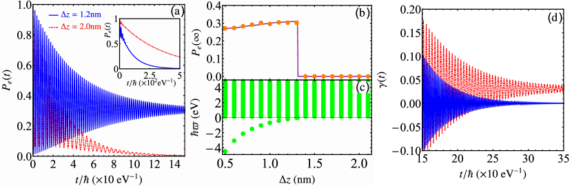
Figure 5: (a) Evolution and (b) long-time values of the excited-state population in different $\Delta z$. The purple line in (b) shows $Z^{2}$ evaluated by the bound state. (c) Energy spectrum of the whole system in different $\Delta z$. (d) Decay rate of the QE in different $\Delta z$. The parameters are chosen as $\hbar\omega_{0}=1.2$ eV, $\hbar\gamma_{0}=10^{-4}$ eV, and $\varepsilon_{\text{d}}=25$. The inset of (a) shows the evolution when $\hbar\gamma_{0}=10^{-6}$ eV. Reproduced figures from [25].

The quantized QE-SPP interaction is studied in Ref. [159] based on the macroscopic quantum electrodynamics. In the vicinity of the nanoparticle-dielectric interface, the spectral density of the SPPs shows a Lorentzian lineshape [160]. Thus, the SPPs is described by an artificially damping cavity. Based on this assumption, a lot of studies on QE-metal nanoparticle hybrid system have been given [161, 162, 163, 164, 165]. However, the Lorentzian spectral density approximation only correctly captures the short-time dynamics of the QEs. On the other hand, due to absorption of the metal to the SPPs, QE coupled to the SPPs tends to its ground state in a long-time limit. It is the main obstacle in the practical application of a hybrid QE-SSP system. Therefore, how to stabilize the coherence of QE is an urgent problem. Recent studies have shown that the formation of the QE-SPP bound states could supply an efficient way to suppress the decoherence of the QE and the damping of the SPPs in the metal [25, 26].

Consider a QE with frequency $\omega_{0}$ placed at a distance $\Delta z$ above the silver interface. The Hamiltonian follows Eq. (1) with the $\bf{k}$-th SPP mode-emitter interaction strength $g_{\bf{k}}=\frac{ic^{-2}\omega_{\bf{k}}^{2}}{\sqrt{\pi\varepsilon_{0}/\hbar}}\int d^{3}\mathbf{r}^{\prime}\sqrt{\text{Im}[\varepsilon_{m}(\omega_{\bf{k}})]}\bm{\mu}\cdot\mathbf{G}(\mathbf{r},\mathbf{r^{\prime}},\omega_{\bf{k}})\cdot\bf{e}_{\bf{k}}$. Here $\varepsilon_{0}$ being the vacuum permittivity, $c$ the speed of light, $\bf{G}(\bf{r},\bf{r}^{\prime},\omega)$ is the Green’s function satisfying the Helmholtz equation $[\nabla\times\nabla\times-\omega^{2}\varepsilon_{m}(\omega)/c^{2}]\mathbf{G}(\mathbf{r},\mathbf{r}^{\prime},\omega)=\delta(\mathbf{r}-\mathbf{r}^{\prime})$, $\bf{r}$ is the position of the emitter with electric dipole $\bm{\mu}$, and $\bf{e}_{\bf{k}}$ is the polarization direction of the SPP mode. Taking the dipole $\bm{\mu}$ along the $z$ direction, the spectral density of the SPPs reads [25]

$$J(\omega)={3\gamma_{0}\sqrt{\varepsilon_{\text{d}}}\omega^{3}\over 4\pi\omega_{0}^{3}}\text{Re}[\int_{0}^{\infty}ds{s^{3}(1-r_{\text{p}}e^{2ik_{z_{\text{d}}}\Delta z})\over\sqrt{1-s^{2}}}],$$ (18)

where $s=k_{\rho}/k_{d}$, $r_{\text{p}}=\frac{\varepsilon_{\text{d}}k_{z_{\text{m}}}-\varepsilon_{\text{m}}(\omega)k_{z_{\text{d}}}}{\varepsilon_{\text{d}}k_{z_{\text{m}}}+\varepsilon_{\text{m}}(\omega)k_{z_{\text{d}}}}$ with $k_{z_{\text{m}}}$ and $k_{z_{\text{d}}}$ being the axial components of the wave vector in the metal and the dielectric, respectively, and $\gamma_{0}=\omega_{0}^{3}\mu/(3\pi\hbar\varepsilon_{0}c^{3})$ is the vacuum spontaneous emission rate. The evolution of the QE obeys Eq. (2). Figure 5 shows the evolution of the excited-state population $P_{e}(t)=\text{Tr}[\hat{\sigma}_{+}\hat{\sigma}_{-}\rho(t)]$ of the QE in different $\Delta z$. When the intrinsic decay rate $\gamma_{0}$ is small, $P_{e}(t)$ monotonically decays to zero, especially for large $\Delta z$ [see the inset of Fig. 5(a)]. When $\gamma_{0}$ is large, the dynamical oscillation becomes significant. It represents a rapid excitation exchange and thus manifests the strong QE-SPP interactions. A remarkable difference between the two results is that although $P_{e}(t)$ approaches zero when $\Delta z=2.0$nm, while it tends to a stable nonzero value when $\Delta z=1.2$nm. It is in sharp contrast to the previous result and represents a dissipation suppression of the QE. Figure 5(b) shows the steady-state population $P_{e}(\infty)$ in different $\Delta z$. It reveals that $P_{e}(\infty)$ matches well with $Z^{2}$ obtained by the bound-state analysis. Figure 5(c) shows clearly that the regions where the QE population is preserved correspond exactly to the one where a bound state is formed in the environmental bandgap. Figure 5(d) is the decay rate $\gamma(t)$ of the QE. The fast oscillations manifest the rapid energy exchange between the QE and the SPPs. It is interesting to see that $\gamma(t)$ asymptotically approaches zero with the formation of the bound state. Such behavior implies that the plasmonic nanostructure in the presence of the bound state can be an ideal platform for the coherent manipulation of QE dynamics, even it is inherently dissipative. This is helpful for utilizing plasmonic nanostructures in quantum devices, such as entanglement generators [166].

The formation of the bound state in the QE-SPPs system also indicates that the SPPs can be used to realize entanglement preservation [26].

3 Quantum control in periodically driven systems

Coherent control via periodic driving dubbed as Floquet engineering has become a versatile tool in artificially synthesizing exotic states of matter in systems of ultracold atoms [167, 168], photonics [169, 170], superconductor qubits [171], and graphene [172]. Different from the static systems, the systems under periodic driving has no well-defined energy spectrum because its energy is not conserved. Floquet theory [173, 174] supplies us with a powerful approach to map a nonequilibrium system under periodic driving to a static one. According to Floquet theory, the periodic system with $\hat{H}(t+T)=\hat{H}(t)$ has a complete set of basis $|\phi_{\alpha}(t)\rangle$ determined by

$$[\hat{H}(t)-i\partial_{t}]|\phi_{\alpha}(t)\rangle=\epsilon_{\alpha}|\phi_{\alpha}(t)\rangle$$ (19)

such that the evolution of any state can be expanded as $|\Psi(t)\rangle=\sum_{\alpha}C_{\alpha}e^{-i\epsilon_{\alpha}t}|\phi_{\alpha}(t)\rangle$ with $C_{\alpha}=\langle u_{\alpha}(0)|\Psi(0)\rangle$. The time-independence of $C_{\alpha}$ implies that $\epsilon_{\alpha}$ and $|\phi_{\alpha}(t)\rangle$ play the same roles in a periodic system as eigenenergies and stationary states do in a static system. They are thus called quasienergies and quasi-stationary states, respectively. Carrying all the quasi-stationary-state characters, the quasienergy spectrum formed by all $\epsilon_{\alpha}$ is a key to study the periodic system. Note that $\epsilon_{\alpha}$ is periodic with period ${2\pi/T}$ because $e^{il\omega t}|u_{\alpha}(t)\rangle$ with $\omega={2\pi/T}$ is also the eigenstate of Eq. (19) with eigenvalue $\epsilon_{\alpha}+l\omega$. It can be proven that the Floquet eigenequation (19) is equivalent to

$$\hat{U}_{T}|\phi_{\alpha}(0)\rangle=e^{-i\epsilon_{\alpha}T}|\phi_{\alpha}(0)\rangle$$ (20)

with $\hat{U}_{T}$ the one-period evolution operator. Thus, the Floquet equation defines an effective static system $\hat{H}_{\text{eff}}=\frac{i}{T}\ln\hat{U}_{T}$ whose eigenvalues are the quasienergies. Then one can engineer the quasienergy spectrum by changing the parameters of the external periodic driving and artificially synthesize many exotic states of matter absent in the static systems. Its merits reside in that the controllability of the systems is dramatically enhanced because time as a new control dimension is introduced to the systems by the periodic driving. This greatly lifts the experimental difficulty in realizing different types of quantum states of matter via changing the intrinsic parameters of the systems, which is hard to be manipulated once the material of the system is fabricated.

In the above section, we reviewed the decoherence control via engineering the bound state in the energy spectrum. A practical difficulty is that one generally cannot change the energy spectrum once the system is explicitly given. In this section, we will review that a parallel decoherence control can be realized by periodic driving as long as a Floquet bound state (FBS) is formed in the quasienergy spectrum. Actually, such engineering to the FBS in the quasienergy spectrum can be generalized to realize artificial topological phases. We will also review its recent progress.

3.1 Floquet control of quantum dissipation

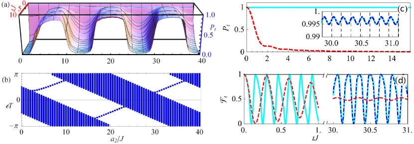
Figure 6: (a) Evolution of $P_{t}$ and (b) quasienergy spectrum of the whole system in different driving amplitude $a_{2}$. The parameters $T=0.25\pi J^{-1}$, $a_{1}=0$, $\tau=0.1\pi J^{-1}$, $g=1.0J$, $\lambda=20.0J$, and $L=800$ are used. Evolution of $P_{t}$ for the initial state $|\phi\rangle=|\uparrow_{0}\rangle$ in (c) and $\mathcal{F}_{t}$ for the initial state $|\phi\rangle=(|\uparrow_{0}\rangle+|\downarrow_{0}\rangle)/\sqrt{2}$ in (d) when $a_{2}=36.0J$ with the FBS (cyan solid line) and $a_{2}=1.5J$ without the FBS (red dashed line). The blue dotdashed lines show the results obtained via analytically evaluating the contribution of the FBS to the asymptotic state. The parameters in (c, d) are $T=0.05\pi J^{-1}$ and $\tau=0.02\pi J^{-1}$. Reproduced figures from [39].

The idea of controlling quantum dissipation via periodic driving is based on the correspondence between the quasienergy spectrum in a temporally periodic system and the energy spectrum in the static system [39]. Compared with the static case, the periodic driving provides a much flexible tool in manipulating the formation of the bound state.

Consider a periodically driven spin-1/2 system interacting with an XX-coupled spin chain environment. The Hamiltonian reads $\hat{H}(t)=\hat{H}_{S}(t)+\hat{H}_{I}+\hat{H}_{E}$ with

$$\hat{H}_{S}(t) = \frac{1}{2}[\lambda+A(t)]\hat{\sigma}_{0}^{z},~{}~{}\hat{H}_{I}=\frac{g}{2}(\hat{\sigma}_{0}^{x}\hat{\sigma}_{1}^{x}+\hat{\sigma}_{0}^{y}\hat{\sigma}_{1}^{y}),$$

$$\hat{H}_{E} = \frac{\lambda}{2}\sum_{j=1}^{L}\hat{\sigma}_{j}^{z}+\frac{J}{2}\sum_{j=1}^{L-1}(\hat{\sigma}_{j}^{x}\hat{\sigma}_{j+1}^{x}+\hat{\sigma}_{j}^{y}\hat{\sigma}_{j+1}^{y}).$$ (21)

Here $\hat{\sigma}^{\alpha}_{j}$ ($\alpha=x,y,z$) being the Pauli matrix of the $j$-th spin, $\lambda$ is the Zeeman interaction induced by the longitudinal magnetic field, $J$ and $g$ are the coupling strengths between the nearest-neighbor spins in the spin chain and the coupling between system spin and the first spin of the chain, respectively, and $L$ is the total number of spins in XX-chain. Here the periodic driving field reads

$$A(t)=\begin{cases}a_{1},&nT<t\leq nT+\tau\\ a_{2},&nT+\tau<t\leq(n+1)T\end{cases},$$ (22)

where $T$ is the driving period, $\tau$ is the duration of the first piece, and $a_{1,2}$ are the driving amplitudes. We consider the initial state as $|\Psi(0)\rangle=|\uparrow_{0}\rangle\otimes|\{\downarrow_{j}\}\rangle$. Because the total excitation number $\hat{\mathcal{N}}=\sum_{j=0}^{L}\hat{\sigma}_{j}^{+}\hat{\sigma}_{j}^{-}$ is conserved, the time-evolved state can be expanded as $|\Psi(t)\rangle=\sum_{j=0}^{L}e^{i\frac{L\lambda t}{2}}c_{j}(t)\hat{\sigma}_{j}^{+}|\{\downarrow_{j}\}\rangle$. Here the excited-state population $P_{t}\equiv|c_{0}(t)|^{2}$ of the system spin is used to characterize the decoherence effect.

Figure 6(a) shows the evolution of $P_{t}$ in different driving amplitude $a_{2}$. When the driving is switched off, i.e., $a_{2}=0$, $P_{t}$ decays monotonically to zero, which means a complete dissipation exerted by the spin chain to the system spin. When the driving is switched on, it is interesting to see that $P_{t}$ is stabilized repeatedly with the increase of $a_{2}$. It is remarkable to see that the regimes where the dissipation is inhibited match well with the ones where the FBS is formed in the quasienergy spectrum [see Fig. 6(b)]. To understand the behavior, we, according to Floquet theory, rewrite $|\Psi(t)\rangle$ as

$$|\Psi(t)\rangle = e^{i{\frac{L\lambda t}{2}}}[xe^{-i\epsilon_{\text{FBS}}t}|\phi_{\text{FBS}}(t)\rangle+\sum_{\alpha\in\text{Band}}y_{\alpha}e^{-i\epsilon_{\alpha}t}|\phi_{\alpha}(t)\rangle],$$ (23)

where $x=\langle\phi_{\text{FBS}}(0)|\Psi(0)\rangle$ and $y_{\alpha}=\langle\phi_{\alpha}(0)|\Psi(0)\rangle$. One can see that $P_{t}$ evolves asymptotically to $P_{\infty}\equiv x^{2}|\langle\Psi(0)|u_{\text{FBS}}(t)\rangle|^{2}$ with all the components in the quasi-energy band vanishing due to the out-of-phase interference contributed by the continuous phases, as confirmed in Fig. 6(c). In the absence of the FBS, $P_{t}$ decays to zero finally. It means that the presence of the FBS would cause $P_{t}$ to survive in the only component of the FBS and thus synchronize with the driving field [175]. For a general initial state $|\phi(0)\rangle=\frac{1}{\sqrt{2}}(|\uparrow_{0}\rangle+|\downarrow_{0}\rangle)$, we use the initial-state fidelity $\mathcal{F}_{t}=\langle\phi(t)|\text{Tr}_{E}[|\Psi(t)\rangle\langle\Psi(t)|]|\phi(0)\rangle$ to reflect the damping of the quantum coherence. The dynamics are shown in Fig. 6(d). In the absence of the FBS, $\mathcal{F}_{t}$ decays to a trivial value $1/2$, which indicates that the system $\rho_{s}=\text{Tr}_{E}[|\Psi(t)\rangle\langle\Psi(t)|]=\frac{\mathbb{I}}{2}$ has no coherence, while $\mathcal{F}_{t}$ shows persistent oscillation once the FBS is formed. The long-time dynamics in Fig. 6(d) verifies again the coincidence of the FBS analysis (blue dashed line) with the exact numerical results (cyan line).

As a stationary state, the bound state in both the static system and the periodically driven system makes the system survive in the only component of the bound state in the long-time limit. Thus, the coherence contained in the bound state is preserved forever. Different from the bound state in a static system, the FBS formed in the quasienergy spectrum itself is temporally periodic. Such periodic driving induced dissipation suppression can be seen as a time-dependent analog to the decoherence suppression induced by the structured environment in spatially periodic photonic crystal setting [176], where the spatial periodicity causes the environment to present a bandgap structure and thus the decoherence of the system is suppressed when the system frequency resides in the bandgap region. However, the temporally periodic driving relaxes greatly the experimental difficulties of the static system in fabricating specific spatial periodicity. Such an FBS mechanism is an exact non-Markovian dynamical control to suppress quantum dissipation by using periodic driving. An optical simulation of this mechanism has been proposed in Ref. [40].

3.2 Floquet control of dissipative quantum battery

A quantum battery (QB) is a device that stores and converts energy at the quantum level [177]. It holds the promises of higher energy-storing density in large-scale integration and faster-charging power than its classical counterpart. A minimal model of QB is described by two coupled two-level systems with one acting as the charger and another as the QB [178, 179]. The Hamiltonian reads

$$\hat{H}_{0}(t)=\hbar\sum_{l=\rm{b},\rm{c}}\omega_{l}\hat{\sigma}^{\dagger}_{l}\hat{\sigma}_{l}+\hbar\kappa f(t)(\hat{\sigma}^{\dagger}_{\text{b}}\hat{\sigma}_{\text{c}}+\text{H.c.}),$$ (24)

where $\hat{\sigma}_{l}=|g\rangle_{l}\langle e|$, with $|g\rangle$ and $|e\rangle$ being the ground and excited states of the two-level systems, are the transition operators of the QB and charger with frequency $\omega_{l}$, and $\kappa$ is their coupling strength. The time-dependent $f(t)$ is a control parameter for the charging, storing, and discharging process that takes

$$f(t)=\left\{\begin{array}[]{ll}1,&nT<t\leq\tau_{c}+nT\\ 0,&nT+\tau_{c}<t\leq nT+(\tau_{s}+\tau_{c})\\ 1,&nT+(\tau_{s}+\tau_{c})<t\leq(n+1)T\\ \end{array}\right.n\in\mathbb{N}.$$ (25)

Here $\tau_{c}$, $\tau_{s}$, and $\tau_{d}$ are the time durations of charging, storing, and discharging, respectively. The initial state of the QB-charger setup is set to $|\psi(0)\rangle=|g_{\rm{b}},e_{\rm{c}}\rangle$. The average energy $\mathcal{E}(t)=\omega_{\rm{b}}\langle\psi(t)|\hat{\sigma}^{\dagger}_{\rm{b}}\hat{\sigma}_{\rm{b}}|\psi(t)\rangle$ of the QB is used to characterize its power, where $|\psi(t)\rangle\equiv\mathcal{T}e^{{-i\over\hbar}\int_{0}^{t}\hat{H}_{0}(\tau)d\tau}|\psi(0)\rangle$ is the evolved state of the QB-charger setup. For the resonant case $\omega_{\rm{b}}=\omega_{\rm{c}}$, with the optimal control time, i.e. $\tau_{c}=\tau_{s}=\tau_{d}=\frac{2\pi}{\kappa}$ [42], the QB-charger setup shows the perfect cyclic evolution: $\mathcal{E}(t)$ reaches its maximal value at the end of each charging step, and empties its total energy at the end of each discharging step. However, in the realistic condition, an invertible power loss is present due to the interactions of the QB and the charger with their respective dissipative environment. It was found that the dissipation causes that energy of QB drop to zero after finite charing-storing-discharging cycles, which is called the aging of the QB [180, 181]. The temporally periodical nature of the cyclic process of the QB inspires us that the detrimental effect of the dissipation on the QB-charger setup can be inhibited by engineering the formation of the FBSs. Then, we review how to reactive the QB under the influences of the dissipative environments by manipulating the FBSs [42].

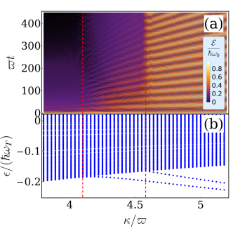
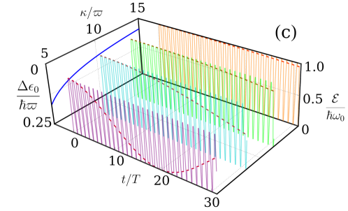
Figure 7: (a) Evolution of the energy of the QB and (b) quasienergy spectrum of the total system in different coupling strength $\kappa$. (c) Evolution of $\mathcal{E}(t)$ in long-time limit and the quasienergy difference $\Delta\epsilon_{0}$ of two FBSs in different $\kappa$. The energy in storage time duration is highlighted by red segments in (c). Other parameters are $N=30$, $\omega_{b}=\omega_{c}=2\varpi$, $g=0.5\varpi$, $q=0.5\varpi$ and $\tau_{c}=\tau_{s}=\tau_{d}=\pi/(2\kappa)$. Reproduced figures from [42].

Consider that the QB and the charger are coupled to two independent environments consisting of an $N\times N$ nearest-neighbor coupled bosonic mode on the square lattice with the mode frequency $\varpi$ and hopping rate $q$ [182]. Their couplings follow Eq. (1) with $\hat{o}\equiv\hat{\sigma}_{\rm{b},(\rm{c})}$, $\omega_{\mathbf{k}}\equiv\varpi-2q(\cos k_{x}+\cos k_{y})$, and the system-environment coupling strength being $g_{\mathbf{k}}=\frac{g}{N}$. Figure 7(a) and (b) show the evolution of $\mathcal{E}(t)$ in different coupling strength $\kappa$ and the corresponding quasienergy spectrum. We can see that the regions where different numbers of FBSs are formed match well with the ones where $\mathcal{E}(t)$ shows different behaviors, i.e. complete decay, energy trapping, and persistent oscillation. When no FBS is formed, $\mathcal{E}(t)$ asymptotically decays to zero. However, when one or two FBSs are formed, $\mathcal{E}(t)$ approaches finite value or shows a persistent oscillation in the long-time limit. According to the Floquet theory, such anomalous dynamical behaviors can be understood by decomposing the evolution state of the total system as $|\Psi(t)\rangle=\sum_{j=1}^{M}c_{j}e^{{-i\over\hbar}\epsilon_{0j}t}|\phi_{0j}(t)\rangle+\sum_{\beta\in\text{CB}}d_{\beta}e^{{-i\over\hbar}\epsilon_{\beta}t}|\phi_{\beta}(t)\rangle$, where $\epsilon$ and $|\phi(t)\rangle$ satisfy Eq. (19), $M$ is the number the FBSs, $c_{j}\equiv\langle\phi_{0j}(0)|\Psi(0)\rangle$ and $d_{\beta}\equiv\langle\phi_{\beta}(0)|\Psi(0)\rangle$. In the long-time limit, the contribution from the continuous energy band to $\mathcal{E}(t)$ approaches zero due to the out-of-phase interference. Then, $\mathcal{E}(\infty)$ reads

$${\mathcal{E}(\infty)\over\hbar\omega_{0}}=\sum_{jj^{\prime}=1}^{M}c_{j}c_{j^{\prime}}^{*}e^{{-i\over\hbar}(\epsilon_{0j}-\epsilon_{0j^{\prime}})t}\langle\phi_{0j^{\prime}}(t)|\hat{\sigma}_{\text{b}}^{\dagger}\hat{\sigma}_{\text{b}}|\phi_{0j}(t)\rangle,$$ (26)

which indicates that the steady behavior of $\mathcal{E}(\infty)$ strongly dependent on the number of FBSs, as shown in Fig. 7(a) and (b). In particular, when $M=2$, $\mathcal{E}(\infty)$ shows the persistent oscillation with multiple frequencies jointly determined by the driven frequency $\omega_{T}$ and the quasienergy difference of two FBSs $\Delta\epsilon_{0}\equiv|\epsilon_{01}-\epsilon_{01}|$. With the bound-state mechanism at hands, it is shown that the QB influenced by the environment can be reactivated by controlling the energy of two FBSs. As shown in Fig. 7(c), with the increasing of $\kappa$, the quasienergy difference asymptotically tends to zero, which reduces the undesired energy oscillation contributed from the interference between two FBSs and thus the QB returns to its near-ideal cyclic stage.

The combination between the decoherence analysis of QB and the Floquet theory supplies an efficient way to overcome the aging problem of the QB via the versatile Floquet engineering. It opens an avenue to build an aging-free QB in practice.

3.3 Floquet control of topological phases

The distinguished role of the periodic driving in engineering bound states in the quasienergy spectrum can also be used to artificially synthesize exotic topological phases [50, 51, 52, 47, 48, 49, 53]. Parallel to the topological phases in the static system, the topological phases in periodically driven systems are called Floquet topological phases. Floquet topological phases defined in the quasienergy spectrum are characterized by a full insulating gap in the bulk and gapless bound states at the edges or the surfaces [183]. The versatility of periodic driving schemes enables us not only to realize topological phases not accessible for the static system in the same setting, but also to explore novel topological phases totally absent in the static system.

Consider a two-band topological system with its parameters periodically driven by a pairwise function with the Hamiltonians read $\mathcal{H}_{1}$ and $\mathcal{H}_{2}$ in the respective time durations $T_{1}$ and $T_{2}$. The coefficient matrices of the Hamiltonians in the operator basis of the momentum space take the form $\mathcal{H}_{j}(\mathbf{k})=\mathbf{h}_{j}(\mathbf{k})\cdot\boldsymbol{\sigma}$ ($j=1,2$) with $\boldsymbol{\sigma}$ being the Pauli matrices. The one-periodic evolution operator reads ${U}_{T}=\varepsilon I_{2\times 2}+i\mathbf{r}\cdot\boldsymbol{\sigma}$ which yield the effective Hamiltonian $\mathcal{H}_{\text{eff}}(\mathbf{k}):=\frac{i}{T}\ln{U}_{T}=\mathbf{h}_{\text{eff}}(\mathbf{k})\cdot\boldsymbol{\sigma}$ with $\mathbf{h}_{\text{eff}}(\mathbf{k})=-\arccos(\varepsilon)\underline{\mathbf{r}}/T$ and [48]

$$\varepsilon = \cos|T_{1}\mathbf{h}_{1}(\mathbf{k})|\cos|T_{2}\mathbf{h}_{2}(\mathbf{k})|-\underline{\mathbf{h}}_{1}\cdot\underline{\mathbf{h}}_{2}\sin|T_{1}\mathbf{h}_{1}(\mathbf{k})|\sin|T_{2}\mathbf{h}_{2}(\mathbf{k})|,$$

$$\mathbf{r} = \underline{\mathbf{h}}_{1}\times\underline{\mathbf{h}}_{2}\sin|T_{1}\mathbf{h}_{1}(\mathbf{k})|\sin|T_{2}\mathbf{h}_{2}(\mathbf{k})|-\underline{\mathbf{h}}_{2}\cos|T_{1}\mathbf{h}_{1}(\mathbf{k})|\sin|T_{2}\mathbf{h}_{2}(\mathbf{k})|$$ (27)

$$-\underline{\mathbf{h}}_{1}\cos|T_{2}\mathbf{h}_{2}(\mathbf{k})|\sin|T_{1}\mathbf{h}_{1}(\mathbf{k})|.$$

Here $T=T_{1}+T_{2}$ and $\underline{\mathbf{v}}\equiv\mathbf{v}/|\mathbf{v}|$ is the unit vector of $\mathbf{v}$. The topological phase transition is associated with the closing and reopening of the quasi-energy bands. One can find from Eqs. (27) that the band gap closing occurs at $\varepsilon=\pm 1$, which is obtained when

$$T_{j}|\mathbf{h}_{j}(\mathbf{k})|=n_{j}\pi,~{}n_{j}\in\mathbb{Z},$$ (28)

$$\text{or}~{}\begin{cases}\underline{\mathbf{h}}_{1}\cdot\underline{\mathbf{h}}_{2}=\pm 1\\ T_{1}|\mathbf{h}_{1}(\mathbf{k})|\pm T_{2}|\mathbf{h}_{2}(\mathbf{k})|=n\pi,~{}n\in\mathbb{Z}\end{cases}$$ (29)

at the quasienergy zero (or $\pi/T$) if $n$ is even (or odd). They give the sufficient condition for judging the occurrence of the Floquet topological phase transition.

3.3.1 Floquet Majorana modes

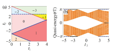
Figure 8: (a) Phase diagram characterized by the winding number when $\mu=-10|\Delta_{1}|$ and $|\Delta_{2}|=2.5|\Delta_{1}|$. (b) Quasienergy spectrum for $t_{1}=|\Delta_{1}|$. The dashed blue line and solid black line stand for two degenerate pairs and a single pair of MMs, respectively. Reproduced figures from [47].

Realizing Majorana modes (MMs) in condensed-matter systems is of vast experimental and theoretical interests due to their potential applications in quantum computation [184, 185, 186, 187, 188]. The zero-bias conductance peaks are regarded as a signature of MMs in spin-orbit coupled semiconductor nanowires [189]. However, they can also be induced by other reasons, e.g. the strong disorder in the nanowire [190, 191] and smooth confinement potential at the wire end [191]. Therefore, more ways to double confirm the formation of MMs in these systems are desired. Studies show that periodic driving can create a widely tunable number of Floquet MMs, which, on the one hand, could dramatically enhance the experimental signal strength, on the other hand, could supply a novel way to identify whether the signal originates from MFs or others by observing its response to the tuning of the driving coefficients [47].

Consider the Kitaev model Hamiltonian for a 1D spinless $p$-wave superconductor

$$H = -\mu\sum_{l=1}^{N}c_{l}^{{\dagger}}c_{l}-\sum_{l=1}^{N-1}(t_{1}c_{l}^{{\dagger}}c_{l+1}+\Delta_{1}c_{l}^{{\dagger}}c_{l+1}^{{\dagger}}+\text{h.c.})-\sum_{l=1}^{N-2}(t_{2}c_{l}^{{\dagger}}c_{l+2}$$ (30)

$$+\Delta_{2}c_{l}^{{\dagger}}c_{l+2}^{{\dagger}}+\text{h.c.}),$$

where $\mu$ is the chemical potential, $t_{a}$ and $\Delta_{a}=\left|\Delta_{a}\right|e^{i\phi_{a}}$ with $a=1$ ($a=2$) describe the nearest- (next-nearest) -neighbor hopping amplitude and pairing potential, respectively, and $\phi_{a}$ is the associated superconducting phases. Its topological characters are dependent on the relative phase $\phi=\phi_{1}-\phi_{2}$ [192]. For $\phi=0$ and $\pi$, $H$ has time-reversal and particle-hole symmetries and its topology is characterized by the winding number, where two pairs of Majorana modes can be generated at most. For other values of $\phi$, $H$ has no time-reversal and particle-hole symmetries and its topology is characterized by a $Z_{2}$ topological invariant, where one pair of Majorana modes is achievable at most.

The periodic driving protocol is designed as follows: in the first half period, $H_{1}=H(\phi_{1},\phi_{2})$ with both $\phi_{1}$ and $\phi_{2}$ fixed; whereas in the second half period, we swap $\phi_{1}$ and $\phi_{2}$ so that $H_{2}=H(\phi_{2},\phi_{1})$. It has been proved that the distinguished action of the periodic driving is that it successfully recovers the time-reversal symmetry and simulates the long-range hopping of the electrons. Thanks to these abilities, an arbitrarily number of MMs is created. Figure 8(a) shows the phase diagram for given driving parameters with the corresponding quasienergy spectrum shown in Fig. 8(b). Compared to the static case which supports at most two pairs of MMs, Floquet engineering provides a feasible method to realize tunable topological edge states. It was reported that more MMs can be induced by increasing the driving period $T$, where longer-range hopping is simulated by the periodic driving [47].

3.3.2 Floquet Chern insulators

The large-Chern-number topological phases have attracted considerable interests [193, 194, 195, 196, 197, 198, 199]. Providing more edge channels, these phases are expected to improve certain device performance by lowering the contact resistance [193, 195]. They can also support multi-mode one-way waveguides, a feature relevant to realizing reflectionless waveguides splitters, combiners, and one-way photonic circuits in photonic crystals [194, 199]. However, a band structure with large Chern numbers is normally hard to be generated in natural material. Special long-range interactions and multi-layered structure of the materials are needed to support such types of exotic phases [200, 201, 196].

Periodic driving widely used in graphene [172], optical lattices [167], and photonic crystals [170] supplies a useful way to create the large-Chern-number topological phases [48]. Consider the Haldane model with up to the third-neighbor hopping included. In the operator basis $C_{\mathbf{k}}=(c_{a\mathbf{k}},c_{b\mathbf{k}})^{T}$, its static Hamiltonian can be written as $H=\sum_{\mathbf{k}\in\text{BZ}}C_{\mathbf{k}}^{{\dagger}}[\mathbf{h}(\mathbf{k})\cdot{\boldsymbol{\sigma}}]C_{\mathbf{k}}$. The associated Bloch vectors $\mathbf{h}(\mathbf{k})$ are

$$\begin{split}&h_{x}(\mathbf{k})=t_{1}[1+\cos(\mathbf{k}\cdot\mathbf{a}_{1})+\cos(\mathbf{k}\cdot\mathbf{a}_{2})]+t_{3}\{2\cos[\mathbf{k}\cdot(\mathbf{a}_{1}-\mathbf{a}_{2})]\\ &~{}~{}~{}~{}~{}~{}~{}~{}~{}~{}+\cos[\mathbf{k}\cdot(\mathbf{a}_{1}+\mathbf{a}_{2})]\},\\ &h_{y}(\mathbf{k})=t_{1}[\sin(\mathbf{k}\cdot\mathbf{a}_{1})+\sin(\mathbf{k}\cdot\mathbf{a}_{2})]+t_{3}\sin[\mathbf{k}\cdot(\mathbf{a}_{1}+\mathbf{a}_{2})],\\ &h_{z}(\mathbf{k})=2t_{2}\sin\phi\{\sin(\mathbf{k}\cdot\mathbf{a}_{1})-\sin(\mathbf{k}\cdot\mathbf{a}_{2})-\sin[\mathbf{k}\cdot(\mathbf{a}_{1}-\mathbf{a}_{2})]\}+M,\end{split}$$ (31)

where $t_{j}$ are the $j$th-neighbor hopping amplitude, $\phi$ is the phase gained by $t_{2}$ hoppings, and $M$ is the mass term. The primitive vectors are $\mathbf{a}_{1}=(\sqrt{3}/2,3/2)$ and $\mathbf{a}_{2}=(-\sqrt{3}/2,3/2)$ in the unit of the hexagonal lattice constant [202]. Figure 9 shows the phase diagram in the $T_{1}$ and $T_{2}$ plane by periodically switching $t_{3}=0.75t_{1}$ and $\phi=-\pi/6$ for duration $T_{1}$ to $t_{3}=-0.75t_{1}$ and $\phi=-\pi/2$ for duration $T_{2}$. A widely tunable Chern numbers with the equal numbers of edge states are generated [see Figs. 9(b) and 9(c)]. Due to the high controllability of the cold atom system [203, 204], a periodic driving scheme was proposed to realize large-topological-number phases via periodically changing the optical lattices [49].

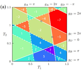
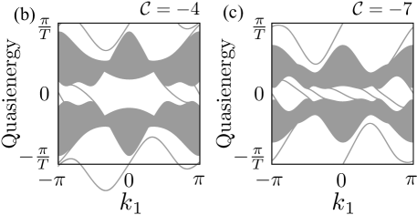
Figure 9: (a) Phase diagram in the $T_{1}$-$T_{2}$ plane obtained by calculating Chern numbers. The phase-boundary lines are analytically obtained from Eqs. (28) and (29). Quasienergy spectra of the periodically Haldane model with $\mathcal{C}=-4$ when $(T_{1},T_{2})=(0.9,1.2)$ in (b) and with $\mathcal{C}=-7$ when $(T_{1},T_{2})=(1.3,1.2)$] in (c). Parameters $t_{2}=0.8t_{1}$ and $M=0$ are used. Reproduced figures from [48].

3.3.3 Non-Hermitian Floquet topological phases

Inspired by the recent experimental realization of topological insulators and the rapid development of non-Hermitian photonics, non-Hermitian topological phases have attracted much attention. From the fundamental physics aspect, people desire to know can the well-developed topological theory in Hermitian systems be generalized to the non-Hermitian cases. This is nontrivial because the skin effect of the non-Hermitian system could cause the breakdown of the bulk-boundary correspondence, which lays the foundation in the topological description in Hermitian systems. From the application aspect, non-Hermitian topological phases have exhibited significant advantages in diverse applications, e.g., laser, invisible media, and sensing [205]. In order to prompt the application of non-Hermitian topological phases, the creation of novel non-Hermitian topological phases in a controllable way via Floquet engineering the system by periodic driving is highly promising. However, the interplay between the non-Hermitian skin effect and periodic driving makes it very hard to characterize the non-Hermitian Floquet topological phases. A recent study has established a complete description of the non-Hermitian Floquet topological phases [53].

Consider the non-Hermitian Su-Schrieffer-Heeger model

$$H=\sum_{l=1}^{L}[(t_{1}+\frac{\gamma}{2})a^{{\dagger}}_{l}b_{l}+(t_{1}-\frac{\gamma}{2})b^{{\dagger}}_{l}a_{l}+t_{2}(a^{{\dagger}}_{l}b_{l-1}+\text{h.c.})],~{}~{}~{}$$ (32)

where $a_{l}$ ($b_{l}$) are the annihilation operators on the sublattice $A$ ($B$) of the $l$th lattice, and $L$ is lattice length. In momentum space and the operator basis $(\tilde{a}_{k},\tilde{b}_{k})^{T}$ with $\tilde{a}_{k}$ ($\tilde{b}_{k}$) being the Fourier transform of $a_{l}$ ($b_{l}$), it reads $\mathcal{H}(k)=d_{x}\sigma_{x}+(d_{y}+i{\gamma}/{2})\sigma_{y}$, where $d_{x}=t_{1}+t_{2}\cos k$ and $d_{y}=t_{2}\sin k$. The bands close at $k=\pi$ (or $0$) when $t_{1}=t_{2}\pm\gamma/2$ (or $-t_{2}\pm\gamma/2$). It is in conflict with the result under the open-boundary condition, where the bands close when $t_{1}=\sqrt{t_{2}^{2}+\gamma^{2}/4}$. It is called the non-Hermiticity caused breakdown of bulk-boundary correspondence [206, 207]. The problem for the static system with chiral symmetry $\sigma^{-1}_{z}\mathcal{H}(k)\sigma_{z}=-\mathcal{H}(k)$ is cured via replacing $e^{ik}$ by $\beta=\sqrt{\lvert\frac{t_{1}-\gamma/2}{t_{1}+\gamma/2}\lvert}e^{ik}$. Then the Hamiltonian is converted into $\mathcal{H}(\beta)=\sum_{n=\pm}R_{n}(\beta)\sigma_{n}$ with $\sigma_{\pm}=(\sigma_{x}\pm i\sigma_{y})/2$ and $R_{\pm}(\beta)=t_{1}\pm\frac{\gamma}{2}+\beta^{\mp 1}t_{2}$. Here $\beta$ defines a generalized Brillouin zone (GBZ). Its topological property is described by the winding number $\mathcal{W}=-(\mathcal{W}_{+}-\mathcal{W}_{-})/2$, where $\mathcal{W}_{\pm}=\frac{1}{2\pi}[\arg R_{\pm}(\beta)]_{C_{\beta}}$ with $[\arg R_{\pm}(\beta)]_{C_{\beta}}$ are the phase change of $R_{\pm}$ as $\beta$ counterclockwisely goes along the GBZ $C_{\beta}$ [208]. When $|t_{1}|<\sqrt{t^{2}_{2}+\gamma^{2}/4}$, $\mathcal{W}=1$ and a pair of edge states is formed.

If the periodic driving

$$t_{2}(t)=\begin{cases}f,&t\in[mT,mT+T_{1})\\ q\,f,&t\in[mT+T_{1},(m+1)T),\end{cases}~{}m\in\mathbb{Z},$$ (33)

is applied to the system, then the chiral symmetry is broken, which makes the GBZ method well developed for the chiral symmetric system not directly applicable. To resolve this problem, two similarity transformations $G_{j}=e^{i(-1)^{j}\mathcal{H}_{j}T_{j}/2}$ are introduced to covert the one-period evolution operator $U_{T}$ into $\tilde{U}_{T,1}=e^{-i\mathcal{H}_{1}T_{1}/2}e^{-i\mathcal{H}_{2}T_{2}}e^{-i\mathcal{H}_{1}T_{1}/2}$ and $\tilde{U}_{T,2}=e^{-i\mathcal{H}_{2}T_{2}/2}e^{-i\mathcal{H}_{1}T_{1}}e^{-i\mathcal{H}_{2}T_{2}/2}$, from which two effective Hamiltonian $\tilde{H}_{\text{eff},j}={i\over T}\ln\tilde{U}_{T,j}$ can be defined. It can be analytically proved that the chiral symmetry is recovered in $\tilde{H}_{\text{eff},j}$. Then after introducing the GBZ $\beta$, two winding numbers $\mathcal{W}_{j}$ associated with $\tilde{\mathcal{H}}_{\text{eff},j}$ can be calculated. The numbers of zero- and $\pi/T$-mode edge sates relate to $\mathcal{W}_{j}$ as $N_{0}=|\mathcal{W}_{1}+\mathcal{W}_{2}|/2$ and $N_{\pi/T}=|\mathcal{W}_{1}-\mathcal{W}_{2}|/2$ [209]. Figure 10(a) shows the quasienergy spectrum under the open-boundary conditions. It is different from the quasienergy spectrum under the periodic-boundary condition, which is called the breakdown of bulk-boundary condition. Although qualitatively capturing the exceptional points of the quasienergy under the periodic-boundary condition, the ill-defined topological numbers from the conventional BZ nonphysically take half integers [see the dashed lines in Fig. 10(b) and 10(c)]. However, the ones from the GBZ correctly count the number of the edge states obtained in the open-boundary condition [see the solid lines in Fig. 10(b) and 10(c)]. Figures 10(d) and 10(e) show the phase diagram in the $T_{1}$-$T_{2}$ plane. A widely tunable number of non-Hermitian edge states are induced by changing the driving parameters.

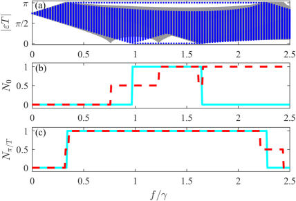
Figure 10: (a) Quasienergy spectra with the change of the driving amplitude under the open (blue lines) and periodic (gray lines) boundary conditions. Numbers of $0$-mode (b) and $\pi/T$-mode (c) edge states defined in the conventional (red dashed) and generalized (cyan solid) BZ. Parameters $t_{1}=2.0\gamma$, $T_{1}=T_{2}=0.6\gamma^{-1}$, $q=3.0$, and $L=80$ are used in (a), (b), and (c). Phase diagram characterized by $\mathcal{W}_{1}$ (d) and $\mathcal{W}_{2}$ (e). The phase boundary lines are obtained from Eqs. (28) and (29). Parameters $t_{1}=1.5\gamma$, $f=2\gamma$, and $q=0$ are used in (d) and (e). Reproduced figures from [53].

All the above results reveal that, without changing the intrinsic parameters in the static system, the periodic driving supplies us another control dimension to adjust the topological edge states. This is useful in the application of topological physics.

4 Conclusion and outlook

In summary, we have reviewed the recent progress on quantum control in open and periodically driven systems. Particular attention has been paid to the distinguished role of bound states in suppressing decoherence of open systems and realizing exotic topological phases in periodically driven systems. It has been revealed that the decoherence of the open system connects tightly with the feature of the energy spectrum of the total system consisting of the open system and its environment. With the formation of a bound state, the decoherence of the open system would be suppressed. It has a profound impact on entanglement preservation, quantum speedup, noncanonical thermalization, quantum metrology, and quantum plasmonics. A parallel result can be established in a periodically driven open system, where the formation of FBSs in the quasienergy spectrum can suppress the dissipation of the open system and the aging of the dissipative quantum battery. It is interesting to see that the controllability of periodic driving on engineering the FBSs can be applied to realize diverse exotic topological phases, e.g. the widely tunable numbers of Majorana modes, Chern insulators, and non-Hermitian topological insulators. The merit of such types of topological phases induced by periodic driving resides in that their controllability is dramatically enhanced because time as a novel control dimension is introduced to the system by periodic driving. It might inspire the exploration of their application via tuning the number of edge/surface states by the periodic driving. The bound state and its distinguished role in the static open-system dynamics have been observed in circuit QED [210, 211] and ultracold atom systems [212]. These progresses provide strong support to the bound-state mechanism and indicate that the profound consequences of the bound reviewed in this article is realizable in the current state of the art. Such experimental feasibility paves the way to beat the decoherence in diverse protocols in quantum technology.

The studies presented in this article hopefully open a number of research lines that deserve to be explored in the future. First, the combination of quantum optics and topological physics has emerged a field called topological quantum optics [213, 214, 215, 216], where the environments interacting with the quantum emitters have topologically nontrivial energy bands. It has potential application in a quantum network. Interesting questions include: Can the system-environment bound states be formed and how the interplay of these bound states with the intrinsic edge states of the environment affects the dynamics of the quantum emitters? Second, parallel to the bound states in the bandgap, the bound states in the continuum are also widely studies [217, 218]. A recent study has showed that the bound states in the continuum can be used to realize the higher-order topological phases [219]. Can they be efficietly manipulated by periodic driving such that more colorful higher-order topological phases are generated in a controllable manner? Third, time crystal is a novel state of matter showing the spontaneous symmetry breaking in the time domain of a quantum system under periodic driving [220, 221]. It arises from the competition of many-body localization due to the disorder against Floquet thermalization under periodic driving [222, 223]. Inspired by the dominated role of bound states in noncanonical thermalization in static systems, a natural question is: Does the avoidance of Floquet thermalization in order to form time crystal is due to the presence of FBSs in quasienergy spectrum? The answer to this question might give the intrinsic physical mechanism to the presence of time crystal from the quasienergy-spectrum feature.

References

- [1] Richard P. Feynman. Simulating physics with computers. Int. J. Theor. Phys., 21(6):467–488, Jun 1982.
- [2] Artur Ekert and Richard Jozsa. Quantum computation and shor’s factoring algorithm. Rev. Mod. Phys., 68:733–753, Jul 1996.
- [3] Jim Law. Quantum computation and quantum information. SIGSOFT Softw. Eng. Notes, 26(4):91, July 2001.
- [4] David P. DiVincenzo. The physical implementation of quantum computation. Fortschritte der Physik, 48(9‐11):771–783, 2000.
- [5] Vittorio Giovannetti, Seth Lloyd, and Lorenzo Maccone. Quantum-enhanced measurements: Beating the standard quantum limit. Science, 306(5700):1330–1336, 2004.
- [6] D. Leibfried, M. D. Barrett, T. Schaetz, J. Britton, J. Chiaverini, W. M. Itano, J. D. Jost, C. Langer, and D. J. Wineland. Toward heisenberg-limited spectroscopy with multiparticle entangled states. Science, 304(5676):1476–1478, 2004.
- [7] Vittorio Giovannetti, Seth Lloyd, and Lorenzo Maccone. Advances in quantum metrology. Nature Photonics, 5(4):222–229, 2011.
- [8] B. M. Escher, R. L. de Matos Filho, and L. Davidovich. General framework for estimating the ultimate precision limit in noisy quantum-enhanced metrology. Nature Physics, 7(5):406–411, 2011.
- [9] I. M. Georgescu, S. Ashhab, and Franco Nori. Quantum simulation. Rev. Mod. Phys., 86:153–185, Mar 2014.
- [10] Charles H. Bennett and Stephen J. Wiesner. Communication via one- and two-particle operators on einstein-podolsky-rosen states. Phys. Rev. Lett., 69:2881–2884, Nov 1992.
- [11] Klaus Mattle, Harald Weinfurter, Paul G. Kwiat, and Anton Zeilinger. Dense coding in experimental quantum communication. Phys. Rev. Lett., 76:4656–4659, Jun 1996.
- [12] Wojciech Hubert Zurek. Decoherence, einselection, and the quantum origins of the classical. Rev. Mod. Phys., 75:715–775, May 2003.
- [13] Charles H. Bennett, Herbert J. Bernstein, Sandu Popescu, and Benjamin Schumacher. Concentrating partial entanglement by local operations. Phys. Rev. A, 53:2046–2052, Apr 1996.
- [14] Zhi Zhao, Jian-Wei Pan, and M. S. Zhan. Practical scheme for entanglement concentration. Phys. Rev. A, 64:014301, Jun 2001.
- [15] Lorenza Viola and Seth Lloyd. Dynamical suppression of decoherence in two-state quantum systems. Phys. Rev. A, 58:2733–2744, Oct 1998.
- [16] G. de Lange, Z. H. Wang, D. Ristè, V. V. Dobrovitski, and R. Hanson. Universal dynamical decoupling of a single solid-state spin from a spin bath. Science, 330(6000):60–63, 2010.
- [17] Seth Lloyd. Coherent quantum feedback. Phys. Rev. A, 62:022108, Jul 2000.
- [18] P. Tombesi and D. Vitali. Macroscopic coherence via quantum feedback. Phys. Rev. A, 51:4913–4917, Jun 1995.
- [19] Sajeev John and Jian Wang. Quantum electrodynamics near a photonic band gap: Photon bound states and dressed atoms. Phys. Rev. Lett., 64:2418–2421, May 1990.
- [20] Shinpei Ogawa, Masahiro Imada, Susumu Yoshimoto, Makoto Okano, and Susumu Noda. Control of light emission by 3d photonic crystals. Science, 305(5681):227–229, 2004.
- [21] Masayuki Fujita, Shigeki Takahashi, Yoshinori Tanaka, Takashi Asano, and Susumu Noda. Simultaneous inhibition and redistribution of spontaneous light emission in photonic crystals. Science, 308(5726):1296–1298, 2005.
- [22] Matthew R. Jorgensen, Jeremy W. Galusha, and Michael H. Bartl. Strongly modified spontaneous emission rates in diamond-structured photonic crystals. Phys. Rev. Lett., 107:143902, Sep 2011.
- [23] D. E. Chang, A. S. Sørensen, P. R. Hemmer, and M. D. Lukin. Quantum optics with surface plasmons. Phys. Rev. Lett., 97(5):1–4, 2006.
- [24] M. S. Tame, K. R. McEnery, K. Özdemir, J. Lee, S. A. Maier, and M. S. Kim. Quantum plasmonics. Nat. Phys., 9(6):329–340, 2013.
- [25] Chun Jie Yang and Jun Hong An. Suppressed dissipation of a quantum emitter coupled to surface plasmon polaritons. Phys. Rev. B, 95(16):5–9, 2017.
- [26] Chun-Jie Yang, Jun-Hong An, and Hai-Qing Lin. Signatures of quantized coupling between quantum emitters and localized surface plasmons. Physical Review Research, 1(2):23027, 2019.
- [27] Manabu Miyamoto. Bound-state eigenenergy outside and inside the continuum for unstable multilevel systems. Phys. Rev. A, 72:063405, Dec 2005.
- [28] Qing-Jun Tong, Jun-Hong An, Hong-Gang Luo, and C. H. Oh. Mechanism of entanglement preservation. Phys. Rev. A, 81:052330, May 2010.
- [29] Ying-Qi Lü, Jun-Hong An, Xi-Meng Chen, Hong-Gang Luo, and C. H. Oh. Frozen gaussian quantum discord in photonic crystal cavity array system. Phys. Rev. A, 88:012129, Jul 2013.
- [30] W. L. Yang, Jun-Hong An, Chengjie Zhang, M. Feng, and C. H. Oh. Preservation of quantum correlation between separated nitrogen-vacancy centers embedded in photonic-crystal cavities. Phys. Rev. A, 87:022312, Feb 2013.
- [31] Chun-Jie Yang, Jun-Hong An, Hong-Gang Luo, Yading Li, and C. H. Oh. Canonical versus noncanonical equilibration dynamics of open quantum systems. Phys. Rev. E, 90:022122, Aug 2014.
- [32] Hai-Bin Liu, W. L. Yang, Jun-Hong An, and Zhen-Yu Xu. Mechanism for quantum speedup in open quantum systems. Phys. Rev. A, 93:020105, Feb 2016.
- [33] Yuan-Sheng Wang, Chong Chen, and Jun-Hong An. Quantum metrology in local dissipative environments. New Journal of Physics, 19(11):113019, nov 2017.
- [34] Kai Bai, Zhen Peng, Hong-Gang Luo, and Jun-Hong An. Retrieving ideal precision in noisy quantum optical metrology. Phys. Rev. Lett., 123:040402, Jul 2019.
- [35] Si-Yuan Bai and Jun-Hong An. Floquet engineering to reactivate a dissipative quantum battery. Phys. Rev. A, 102:060201(R), Dec 2020.
- [36] J. F. Poyatos, J. I. Cirac, and P. Zoller. Quantum reservoir engineering with laser cooled trapped ions. Phys. Rev. Lett., 77:4728–4731, Dec 1996.
- [37] A. Metelmann and A. A. Clerk. Nonreciprocal photon transmission and amplification via reservoir engineering. Phys. Rev. X, 5:021025, Jun 2015.
- [38] Takashi Oka and Sota Kitamura. Floquet engineering of quantum materials. Annual Review of Condensed Matter Physics, 10(1):387–408, 2019.
- [39] Chong Chen, Jun-Hong An, Hong-Gang Luo, C. P. Sun, and C. H. Oh. Floquet control of quantum dissipation in spin chains. Phys. Rev. A, 91:052122, May 2015.
- [40] Chao Ma, Yuan-Sheng Wang, and Jun-Hong An. Floquet engineering of localized propagation of light in a waveguide array. Phys. Rev. A, 97:023808, Feb 2018.
- [41] W L Yang, W L Song, Jun-Hong An, M Feng, D Suter, and Jiangfeng Du. Floquet engineering to entanglement protection of distant nitrogen vacancy centers. New Journal of Physics, 21(1):013007, jan 2019.
- [42] Si-Yuan Bai and Jun-Hong An. Floquet engineering to reactivate a dissipative quantum battery. 2020.
- [43] Milena Grifoni and Peter Hänggi. Driven quantum tunneling. Physics Reports, 304(5):229 – 354, 1998.
- [44] M. Thorwart, L. Hartmann, I. Goychuk, and P. Hänggi. Controlling decoherence of a two-level atom in a lossy cavity. null, 47(14-15):2905–2919, November 2000.
- [45] Sigmund Kohler, Jörg Lehmann, and Peter Hänggi. Driven quantum transport on the nanoscale. Physics Reports, 406(6):379 – 443, 2005.
- [46] Netanel H. Lindner, Gil Refael, and Victor Galitski. Floquet topological insulator in semiconductor quantum wells. Nature Physics, 7(6):490–495, 2011.
- [47] Qing-Jun Tong, Jun-Hong An, Jiangbin Gong, Hong-Gang Luo, and C. H. Oh. Generating many majorana modes via periodic driving: A superconductor model. Phys. Rev. B, 87:201109, May 2013.
- [48] Tian-Shi Xiong, Jiangbin Gong, and Jun-Hong An. Towards large-chern-number topological phases by periodic quenching. Phys. Rev. B, 93:184306, May 2016.
- [49] Hui Liu, Tian-Shi Xiong, Wei Zhang, and Jun-Hong An. Floquet engineering of exotic topological phases in systems of cold atoms. Phys. Rev. A, 100:023622, Aug 2019.
- [50] Mark S. Rudner, Netanel H. Lindner, Erez Berg, and Michael Levin. Anomalous edge states and the bulk-edge correspondence for periodically driven two-dimensional systems. Phys. Rev. X, 3:031005, Jul 2013.
- [51] Arijit Kundu, H. A. Fertig, and Babak Seradjeh. Effective theory of floquet topological transitions. Phys. Rev. Lett., 113:236803, Dec 2014.
- [52] Mahmoud Lababidi, Indubala I. Satija, and Erhai Zhao. Counter-propagating edge modes and topological phases of a kicked quantum hall system. Phys. Rev. Lett., 112:026805, Jan 2014.
- [53] Hong Wu and Jun-Hong An. Floquet topological phases of non-hermitian systems. Phys. Rev. B, 102:041119, Jul 2020.
- [54] Jérôme Cayssol, Balázs Dóra, Ferenc Simon, and Roderich Moessner. Floquet topological insulators. physica status solidi (RRL) – Rapid Research Letters, 7(1‐2):101–108, 2013.
- [55] Sebabrata Mukherjee, Alexander Spracklen, Manuel Valiente, Erika Andersson, Patrik Öhberg, Nathan Goldman, and Robert R. Thomson. Experimental observation of anomalous topological edge modes in a slowly driven photonic lattice. Nature Communications, 8(1):13918, 2017.
- [56] M.O. Scully and M.S. Zubairy. Quantum Optics. Cambridge University Press, 1997.
- [57] Alexander V. Khaetskii, Daniel Loss, and Leonid Glazman. Electron spin decoherence in quantum dots due to interaction with nuclei. Phys. Rev. Lett., 88:186802, Apr 2002.
- [58] I. A. Merkulov, Al. L. Efros, and M. Rosen. Electron spin relaxation by nuclei in semiconductor quantum dots. Phys. Rev. B, 65:205309, Apr 2002.
- [59] V. Bouchiat, D. Vion, P. Joyez, D. Esteve, and M. H. Devoret. Quantum coherence with a single cooper pair. Physica Scripta, T76(1):165, 1998.
- [60] I. R. Senitzky. Dissipation in quantum mechanics. the harmonic oscillator. Phys. Rev., 119:670–679, Jul 1960.
- [61] I. R. Senitzky. Dissipation in quantum mechanics. the harmonic oscillator. ii. Phys. Rev., 124:642–648, Nov 1961.
- [62] Inés de Vega and Daniel Alonso. Dynamics of non-markovian open quantum systems. Rev. Mod. Phys., 89:015001, Jan 2017.
- [63] A. Kossakowski. On quantum statistical mechanics of non-hamiltonian systems. Reports on Mathematical Physics, 3(4):247 – 274, 1972.
- [64] Peter Zoller Crispin Gardiner. Quantum noise: A Handbook of Markovian and Non-Markovian Quantum Stochastic Methods with Applications to Quantum Optics. Springer series in synergetics. Springer, 2nd enlarged ed edition, 2004.
- [65] Jay R. Ackerhalt, Peter L. Knight, and Joseph H. Eberly. Radiation reaction and radiative frequency shifts. Phys. Rev. Lett., 30:456–460, Mar 1973.
- [66] G. Ithier, E. Collin, P. Joyez, P. J. Meeson, D. Vion, D. Esteve, F. Chiarello, A. Shnirman, Y. Makhlin, J. Schriefl, and G. Schön. Decoherence in a superconducting quantum bit circuit. Phys. Rev. B, 72:134519, Oct 2005.
- [67] Heinz-Peter Breuer, Elsi-Mari Laine, Jyrki Piilo, and Bassano Vacchini. Colloquium: Non-markovian dynamics in open quantum systems. Rev. Mod. Phys., 88:021002, Apr 2016.
- [68] R. P. Feynman and F. L. Vernon. The theory of a general quantum system interacting with a linear dissipative system. Annals of Physics, 24:118 – 173, 1963.
- [69] Jun-Hong An and Wei-Min Zhang. Non-markovian entanglement dynamics of noisy continuous-variable quantum channels. Phys. Rev. A, 76:042127, Oct 2007.
- [70] A. J. Leggett, S. Chakravarty, A. T. Dorsey, Matthew P. A. Fisher, Anupam Garg, and W. Zwerger. Dynamics of the dissipative two-state system. Rev. Mod. Phys., 59:1–85, Jan 1987.
- [71] A. Einstein, B. Podolsky, and N. Rosen. Can quantum-mechanical description of physical reality be considered complete? Phys. Rev., 47:777–780, May 1935.
- [72] Ryszard Horodecki, Paweł Horodecki, Michał Horodecki, and Karol Horodecki. Quantum entanglement. Rev. Mod. Phys., 81:865–942, Jun 2009.
- [73] Charles H. Bennett and Gilles Brassard. Quantum cryptography: Public key distribution and coin tossing. Theoretical Computer Science, 560:7 – 11, 2014. Theoretical Aspects of Quantum Cryptography: celebrating 30 years of BB84.
- [74] Artur K. Ekert. Quantum cryptography based on bell’s theorem. Phys. Rev. Lett., 67:661–663, Aug 1991.
- [75] Nicolas Gisin, Grégoire Ribordy, Wolfgang Tittel, and Hugo Zbinden. Quantum cryptography. Rev. Mod. Phys., 74:145–195, Mar 2002.
- [76] Ting Yu and J. H. Eberly. Finite-time disentanglement via spontaneous emission. Phys. Rev. Lett., 93:140404, Sep 2004.
- [77] M. P. Almeida, F. de Melo, M. O. Hor-Meyll, A. Salles, S. P. Walborn, P. H. Souto Ribeiro, and L. Davidovich. Experimental observation of environment-induced sudden death of entanglement. In Leon Cohen, editor, Noise and Fluctuations in Photonics, Quantum Optics, and Communications, volume 6603, pages 320 – 332. International Society for Optics and Photonics, SPIE, 2007.
- [78] Ting Yu and J. H. Eberly. Sudden death of entanglement. Science, 323(5914):598–601, 2009.
- [79] B. Bellomo, R. Lo Franco, and G. Compagno. Entanglement dynamics of two independent qubits in environments with and without memory. Phys. Rev. A, 77:032342, Mar 2008.
- [80] Sabrina Maniscalco, Francesco Francica, Rosa L. Zaffino, Nicola Lo Gullo, and Francesco Plastina. Protecting entanglement via the quantum zeno effect. Phys. Rev. Lett., 100:090503, Mar 2008.
- [81] Jin-Shi Xu, Chuan-Feng Li, Ming Gong, Xu-Bo Zou, Cheng-Hao Shi, Geng Chen, and Guang-Can Guo. Experimental demonstration of photonic entanglement collapse and revival. Phys. Rev. Lett., 104:100502, Mar 2010.
- [82] Bruno Bellomo, Rosario Lo Franco, Sabrina Maniscalco, and Giuseppe Compagno. Entanglement trapping in structured environments. Phys. Rev. A, 78:060302, Dec 2008.
- [83] Qing-Jun Tong, Jun-Hong An, Hong-Gang Luo, and C H Oh. Decoherence suppression of a dissipative qubit by the non-markovian effect. Journal of Physics B: Atomic, Molecular and Optical Physics, 43(15):155501, jul 2010.
- [84] William K. Wootters. Entanglement of formation of an arbitrary state of two qubits. Phys. Rev. Lett., 80:2245–2248, Mar 1998.
- [85] Roland Hildebrand. Concurrence revisited. J. Math. Phys., 48(10):102108, 2007.
- [86] Jun-Hong An, Ye Yeo, Wei-Min Zhang, and C H Oh. Entanglement oscillation and survival induced by non-markovian decoherence dynamics of the entangled squeezed state. Journal of Physics A: Mathematical and Theoretical, 42(1):015302, nov 2008.
- [87] J. Anandan and Y. Aharonov. Geometry of quantum evolution. Phys. Rev. Lett., 65:1697–1700, Oct 1990.
- [88] Leonid Mandelstam and IG Tamm. The uncertainty relation between energy and time in non-relativistic quantum mechanics. In Selected Papers, pages 115–123. Springer, 1991.
- [89] Vaidman L. Minimum time for the evolution to an orthogonal quantum state. American Journal of Physics, 60(2):182–183, 1992.
- [90] Seth Lloyd. Ultimate physical limits to computation. Nature, 406(6799):1047–1054, 2000.
- [91] Shunlong Luo. How fast can a quantum state evolve into a target state? Physica D: Nonlinear Phenomena, 189(1):1 – 7, 2004.
- [92] Norman Margolus and Lev B. Levitin. The maximum speed of dynamical evolution. Physica D: Nonlinear Phenomena, 120(1):188 – 195, 1998. Proceedings of the Fourth Workshop on Physics and Consumption.
- [93] M. M. Taddei, B. M. Escher, L. Davidovich, and R. L. de Matos Filho. Quantum speed limit for physical processes. Phys. Rev. Lett., 110:050402, Jan 2013.
- [94] A. del Campo, I. L. Egusquiza, M. B. Plenio, and S. F. Huelga. Quantum speed limits in open system dynamics. Phys. Rev. Lett., 110:050403, Jan 2013.
- [95] Diego Paiva Pires, Marco Cianciaruso, Lucas C. Céleri, Gerardo Adesso, and Diogo O. Soares-Pinto. Generalized geometric quantum speed limits. Phys. Rev. X, 6:021031, Jun 2016.
- [96] Sebastian Deffner and Eric Lutz. Generalized clausius inequality for nonequilibrium quantum processes. Phys. Rev. Lett., 105:170402, Oct 2010.
- [97] S. Alipour, M. Mehboudi, and A. T. Rezakhani. Quantum metrology in open systems: Dissipative cramér-rao bound. Phys. Rev. Lett., 112:120405, Mar 2014.
- [98] Miroslav Gajdacz, Kunal K. Das, Jan Arlt, Jacob F. Sherson, and Tomá š Opatrný. Time-limited optimal dynamics beyond the quantum speed limit. Phys. Rev. A, 92:062106, Dec 2015.
- [99] Minh C. Tran, Chi-Fang Chen, Adam Ehrenberg, Andrew Y. Guo, Abhinav Deshpande, Yifan Hong, Zhe-Xuan Gong, Alexey V. Gorshkov, and Andrew Lucas. Hierarchy of linear light cones with long-range interactions. Phys. Rev. X, 10:031009, Jul 2020.
- [100] Man-Hong Yung. Quantum speed limit for perfect state transfer in one dimension. Phys. Rev. A, 74:030303, Sep 2006.
- [101] Sebastian Deffner and Eric Lutz. Quantum speed limit for non-markovian dynamics. Phys. Rev. Lett., 111:010402, Jul 2013.
- [102] A. D. Cimmarusti, Z. Yan, B. D. Patterson, L. P. Corcos, L. A. Orozco, and S. Deffner. Environment-assisted speed-up of the field evolution in cavity quantum electrodynamics. Phys. Rev. Lett., 114:233602, Jun 2015.
- [103] Heinz-Peter Breuer, Elsi-Mari Laine, and Jyrki Piilo. Measure for the degree of non-markovian behavior of quantum processes in open systems. Phys. Rev. Lett., 103:210401, Nov 2009.
- [104] Sandu Popescu, Anthony J. Short, and Andreas Winter. Entanglement and the foundations of statistical mechanics. Nature Physics, 2(11):754–758, 2006.
- [105] Noah Linden, Sandu Popescu, Anthony J. Short, and Andreas Winter. Quantum mechanical evolution towards thermal equilibrium. Phys. Rev. E, 79:061103, Jun 2009.
- [106] Hal Tasaki. From quantum dynamics to the canonical distribution: General picture and a rigorous example. Phys. Rev. Lett., 80:1373–1376, Feb 1998.
- [107] Sheldon Goldstein, Joel L. Lebowitz, Roderich Tumulka, and Nino Zanghì. Canonical typicality. Phys. Rev. Lett., 96:050403, Feb 2006.
- [108] Peter Reimann. Canonical thermalization. New J. Phys., 12(5):055027, may 2010.
- [109] Oleg Lychkovskiy. Necessary condition for the thermalization of a quantum system coupled to a quantum bath. Phys. Rev. E, 82:011123, Jul 2010.
- [110] Chee Kong Lee, Jianshu Cao, and Jiangbin Gong. Noncanonical statistics of a spin-boson model: Theory and exact monte carlo simulations. Phys. Rev. E, 86:021109, Aug 2012.
- [111] S. Genway, A. F. Ho, and D. K. K. Lee. Dynamics of thermalization and decoherence of a nanoscale system. Phys. Rev. Lett., 111:130408, Sep 2013.
- [112] Marcos Rigol, Vanja Dunjko, and Maxim Olshanii. Thermalization and its mechanism for generic isolated quantum systems. Nature, 452(7189):854–858, 2008.
- [113] A. V. Ponomarev, S. Denisov, and P. Hänggi. Thermal equilibration between two quantum systems. Phys. Rev. Lett., 106:010405, Jan 2011.
- [114] M. C. Bañuls, J. I. Cirac, and M. B. Hastings. Strong and weak thermalization of infinite nonintegrable quantum systems. Phys. Rev. Lett., 106:050405, Feb 2011.
- [115] Anatoli Polkovnikov, Krishnendu Sengupta, Alessandro Silva, and Mukund Vengalattore. Colloquium: Nonequilibrium dynamics of closed interacting quantum systems. Rev. Mod. Phys., 83:863–883, Aug 2011.
- [116] Eitan Geva, Efrat Rosenman, and David Tannor. On the second-order corrections to the quantum canonical equilibrium density matrix. The Journal of Chemical Physics, 113(4):1380–1390, 2000.
- [117] Takashi Mori and Seiji Miyashita. Dynamics of the density matrix in contact with a thermal bath and the quantum master equation. Journal of the Physical Society of Japan, 77(12):124005, 2008.
- [118] Y. Subasi, C. H. Fleming, J. M. Taylor, and B. L. Hu. Equilibrium states of open quantum systems in the strong coupling regime. Phys. Rev. E, 86:061132, Dec 2012.
- [119] D. Pagel, A. Alvermann, and H. Fehske. Equilibration and thermalization of the dissipative quantum harmonic oscillator in a nonthermal environment. Phys. Rev. E, 87:012127, Jan 2013.
- [120] A. Rançon and J. Bonart. Exact dynamics and thermalization of an open bosonic quantum system in the presence of a quantum phase transition induced by the environment. Europhys. Lett., 104(5):50010, dec 2013.
- [121] Ulrich Hoeppe, Christian Wolff, Jens Küchenmeister, Jens Niegemann, Malte Drescher, Hartmut Benner, and Kurt Busch. Direct observation of non-markovian radiation dynamics in 3d bulk photonic crystals. Phys. Rev. Lett., 108:043603, Jan 2012.
- [122] H. Tahara, Y. Ogawa, and F. Minami. Non-markovian dynamics of spectral narrowing for excitons in the layered semiconductor gase observed using optical four-wave mixing spectroscopy. Phys. Rev. Lett., 107:037402, Jul 2011.
- [123] Christophe Galland, Alexander Högele, Hakan E. Türeci, and Ata ç Imamoğlu. Non-markovian decoherence of localized nanotube excitons by acoustic phonons. Phys. Rev. Lett., 101:067402, Aug 2008.
- [124] Bi-Heng Liu, Li Li, Yun-Feng Huang, Chuan-Feng Li, Guang-Can Guo, Elsi-Mari Laine, Heinz-Peter Breuer, and Jyrki Piilo. Experimental control of the transition from markovian to non-markovian dynamics of open quantum systems. Nature Physics, 7(12):931–934, December 2011.
- [125] K. H. Madsen, S. Ates, T. Lund-Hansen, A. Löffler, S. Reitzenstein, A. Forchel, and P. Lodahl. Observation of non-markovian dynamics of a single quantum dot in a micropillar cavity. Phys. Rev. Lett., 106:233601, Jun 2011.
- [126] Hai-Bin Liu, Jun-Hong An, Chong Chen, Qing-Jun Tong, Hong-Gang Luo, and C. H. Oh. Anomalous decoherence in a dissipative two-level system. Phys. Rev. A, 87:052139, May 2013.
- [127] Vittorio Giovannetti, Seth Lloyd, and Lorenzo Maccone. Quantum metrology. Phys. Rev. Lett., 96:010401, Jan 2006.
- [128] Samuel L. Braunstein and Carlton M. Caves. Statistical distance and the geometry of quantum states. Phys. Rev. Lett., 72:3439–3443, May 1994.
- [129] C. L. Degen, F. Reinhard, and P. Cappellaro. Quantum sensing. Rev. Mod. Phys., 89:035002, Jul 2017.
- [130] Luca Pezzè, Augusto Smerzi, Markus K. Oberthaler, Roman Schmied, and Philipp Treutlein. Quantum metrology with nonclassical states of atomic ensembles. Rev. Mod. Phys., 90:035005, Sep 2018.
- [131] M. et al. Tse. Quantum-enhanced advanced ligo detectors in the era of gravitational-wave astronomy. Phys. Rev. Lett., 123:231107, Dec 2019.
- [132] F. et al. Acernese. Increasing the astrophysical reach of the advanced virgo detector via the application of squeezed vacuum states of light. Phys. Rev. Lett., 123:231108, Dec 2019.
- [133] Andrew D. Ludlow, Martin M. Boyd, Jun Ye, E. Peik, and P. O. Schmidt. Optical atomic clocks. Rev. Mod. Phys., 87:637–701, Jun 2015.
- [134] I. Kruse, K. Lange, J. Peise, B. Lücke, L. Pezzè, J. Arlt, W. Ertmer, C. Lisdat, L. Santos, A. Smerzi, and C. Klempt. Improvement of an atomic clock using squeezed vacuum. Phys. Rev. Lett., 117:143004, Sep 2016.
- [135] S. F. Huelga, C. Macchiavello, T. Pellizzari, A. K. Ekert, M. B. Plenio, and J. I. Cirac. Improvement of frequency standards with quantum entanglement. Phys. Rev. Lett., 79:3865–3868, Nov 1997.
- [136] Yuichiro Matsuzaki, Simon C. Benjamin, and Joseph Fitzsimons. Magnetic field sensing beyond the standard quantum limit under the effect of decoherence. Phys. Rev. A, 84:012103, Jul 2011.
- [137] Alex W. Chin, Susana F. Huelga, and Martin B. Plenio. Quantum metrology in non-markovian environments. Phys. Rev. Lett., 109:233601, Dec 2012.
- [138] Katarzyna Macieszczak. Zeno limit in frequency estimation with non-markovian environments. Phys. Rev. A, 92:010102, Jul 2015.
- [139] Carlton M. Caves. Quantum-mechanical noise in an interferometer. Phys. Rev. D, 23:1693–1708, Apr 1981.
- [140] A. V. Kabashin, P. Evans, S. Pastkovsky, W. Hendren, G. A. Wurtz, R. Atkinson, R. Pollard, V. A. Podolskiy, and A. V. Zayats. Plasmonic nanorod metamaterials for biosensing. Nature Materials, 8(11):867–871, 2009.
- [141] Harry A. Atwater and Albert Polman. Plasmonics for improved photovoltaic devices. Nature Materials, 9(3):205–213, 2010.
- [142] Vincenzo Giannini, Antonio I. Fernández-Domínguez, Susannah C. Heck, and Stefan A. Maier. Plasmonic nanoantennas: Fundamentals and their use in controlling the radiative properties of nanoemitters. Chem. Rev., 111(6):3888–3912, June 2011.
- [143] Yih Hong Lee, Wenxiong Shi, Hiang Kwee Lee, Ruibin Jiang, In Yee Phang, Yan Cui, Lucio Isa, Yijie Yang, Jianfang Wang, Shuzhou Li, and Xing Yi Ling. Nanoscale surface chemistry directs the tunable assembly of silver octahedra into three two-dimensional plasmonic superlattices. Nature Communications, 6(1):6990, 2015.
- [144] J M Pitarke, V M Silkin, E V Chulkov, and P M Echenique. Theory of surface plasmons and surface-plasmon polaritons. Reports on Progress in Physics, 70(1):1–87, dec 2006.
- [145] Adriano Cacciola, Omar Di Stefano, Roberto Stassi, Rosalba Saija, and Salvatore Savasta. Ultrastrong coupling of plasmons and excitons in a nanoshell. ACS Nano, 8(11):11483–11492, November 2014.
- [146] S. Aberra Guebrou, C. Symonds, E. Homeyer, J. C. Plenet, Yu. N. Gartstein, V. M. Agranovich, and J. Bellessa. Coherent emission from a disordered organic semiconductor induced by strong coupling with surface plasmons. Phys. Rev. Lett., 108:066401, Feb 2012.
- [147] P. Törmä and W. L. Barnes. Strong coupling between surface plasmon polaritons and emitters: a review. Reports on Progress in Physics, 78(1):013901, dec 2014.
- [148] A. González-Tudela, P. A. Huidobro, L. Martín-Moreno, C. Tejedor, and F. J. García-Vidal. Theory of strong coupling between quantum emitters and propagating surface plasmons. Phys. Rev. Lett., 110:126801, Mar 2013.
- [149] William L Barnes. Surface plasmon–polariton length scales: a route to sub-wavelength optics. Journal of Optics A: Pure and Applied Optics, 8(4):S87–S93, mar 2006.
- [150] Edward D. Palik Edward D. Palik. Handbook of Optical Constants of Solids, volume Volumes 1-4 of Academic Press Handbook. Academic Press, 1985.
- [151] William L. Barnes, Alain Dereux, and Thomas W. Ebbesen. Surface plasmon subwavelength optics. Nature, 424(6950):824–830, 2003.
- [152] Andreas Trügler and Ulrich Hohenester. Strong coupling between a metallic nanoparticle and a single molecule. Phys. Rev. B, 77:115403, Mar 2008.
- [153] Martin Wersäll, Jorge Cuadra, Tomasz J. Antosiewicz, Sinan Balci, and Timur Shegai. Observation of mode splitting in photoluminescence of individual plasmonic nanoparticles strongly coupled to molecular excitons. Nano Lett., 17(1):551–558, January 2017.
- [154] Denis G. Baranov, Martin Wersäll, Jorge Cuadra, Tomasz J. Antosiewicz, and Timur Shegai. Novel nanostructures and materials for strong light-matter interactions. ACS Photonics, 5(1):24–42, January 2018.
- [155] Rohit Chikkaraddy, Bart de Nijs, Felix Benz, Steven J. Barrow, Oren A. Scherman, Edina Rosta, Angela Demetriadou, Peter Fox, Ortwin Hess, and Jeremy J. Baumberg. Single-molecule strong coupling at room temperature in plasmonic nanocavities. Nature, 535(7610):127–130, 2016.
- [156] Korenobu Matsuzaki, Simon Vassant, Hsuan-Wei Liu, Anke Dutschke, Björn Hoffmann, Xuewen Chen, Silke Christiansen, Matthew R. Buck, Jennifer A. Hollingsworth, Stephan Götzinger, and Vahid Sandoghdar. Strong plasmonic enhancement of biexciton emission: controlled coupling of a single quantum dot to a gold nanocone antenna. Scientific Reports, 7(1):42307, 2017.
- [157] Günter Kewes, Felix Binkowski, Sven Burger, Lin Zschiedrich, and Oliver Benson. Heuristic modeling of strong coupling in plasmonic resonators. ACS Photonics, 5(10):4089–4097, October 2018.
- [158] Parinda Vasa and Christoph Lienau. Strong light-matter interaction in quantum emitter/metal hybrid nanostructures. ACS Photonics, 5(1):2–23, January 2018.
- [159] T. Gruner and D.-G. Welsch. Green-function approach to the radiation-field quantization for homogeneous and inhomogeneous kramers-kronig dielectrics. Phys. Rev. A, 53:1818–1829, Mar 1996.
- [160] Edo Waks and Deepak Sridharan. Cavity qed treatment of interactions between a metal nanoparticle and a dipole emitter. Phys. Rev. A, 82:043845, Oct 2010.
- [161] Raman A. Shah, Norbert F. Scherer, Matthew Pelton, and Stephen K. Gray. Ultrafast reversal of a fano resonance in a plasmon-exciton system. Phys. Rev. B, 88:075411, Aug 2013.
- [162] A. Delga, J. Feist, J. Bravo-Abad, and F. J. Garcia-Vidal. Quantum emitters near a metal nanoparticle: Strong coupling and quenching. Phys. Rev. Lett., 112:253601, Jun 2014.
- [163] Rong-Chun Ge and Stephen Hughes. Quantum dynamics of two quantum dots coupled through localized plasmons: An intuitive and accurate quantum optics approach using quasinormal modes. Phys. Rev. B, 92:205420, Nov 2015.
- [164] Rui-Qi Li, D. Hernángomez-Pérez, F. J. García-Vidal, and A. I. Fernández-Domínguez. Transformation optics approach to plasmon-exciton strong coupling in nanocavities. Phys. Rev. Lett., 117:107401, Aug 2016.
- [165] Pai Peng, Yong-Chun Liu, Da Xu, Qi-Tao Cao, Guowei Lu, Qihuang Gong, and Yun-Feng Xiao. Enhancing coherent light-matter interactions through microcavity-engineered plasmonic resonances. Phys. Rev. Lett., 119:233901, Dec 2017.
- [166] A. Gonzalez-Tudela, D. Martin-Cano, E. Moreno, L. Martin-Moreno, C. Tejedor, and F. J. Garcia-Vidal. Entanglement of two qubits mediated by one-dimensional plasmonic waveguides. Phys. Rev. Lett., 106:020501, Jan 2011.
- [167] André Eckardt. Colloquium: Atomic quantum gases in periodically driven optical lattices. Rev. Mod. Phys., 89:011004, Mar 2017.
- [168] F. Meinert, M. J. Mark, K. Lauber, A. J. Daley, and H.-C. Nägerl. Floquet engineering of correlated tunneling in the bose-hubbard model with ultracold atoms. Phys. Rev. Lett., 116:205301, May 2016.
- [169] Mikael C. Rechtsman, Julia M. Zeuner, Yonatan Plotnik, Yaakov Lumer, Daniel Podolsky, Felix Dreisow, Stefan Nolte, Mordechai Segev, and Alexander Szameit. Photonic floquet topological insulators. Nature, 496(7444):196–200, 2013.
- [170] Qingqing Cheng, Yiming Pan, Huaiqiang Wang, Chaoshi Zhang, Dong Yu, Avi Gover, Haijun Zhang, Tao Li, Lei Zhou, and Shining Zhu. Observation of anomalous modes in photonic floquet engineering. Phys. Rev. Lett., 122:173901, May 2019.
- [171] P. Roushan, C. Neill, A. Megrant, Y. Chen, R. Babbush, R. Barends, B. Campbell, Z. Chen, B. Chiaro, A. Dunsworth, A. Fowler, E. Jeffrey, J. Kelly, E. Lucero, J. Mutus, P. J. J. OHuo Heng alley, M. Neeley, C. Quintana, D. Sank, A. Vainsencher, J. Wenner, T. White, E. Kapit, H. Neven, and J. Martinis. Chiral ground-state currents of interacting photons in a synthetic magnetic field. Nature Physics, 13(2):146–151, 2017.
- [172] J. W. McIver, B. Schulte, F.-U. Stein, T. Matsuyama, G. Jotzu, G. Meier, and A. Cavalleri. Light-induced anomalous hall effect in graphene. Nature Physics, 16(1):38–41, 2020.
- [173] Jon H. Shirley. Solution of the schrödinger equation with a hamiltonian periodic in time. Phys. Rev., 138:B979–B987, May 1965.
- [174] Hideo Sambe. Steady states and quasienergies of a quantum-mechanical system in an oscillating field. Phys. Rev. A, 7:2203–2213, Jun 1973.
- [175] Angelo Russomanno, Alessandro Silva, and Giuseppe E. Santoro. Periodic steady regime and interference in a periodically driven quantum system. Phys. Rev. Lett., 109:257201, Dec 2012.
- [176] M. D. Leistikow, A. P. Mosk, E. Yeganegi, S. R. Huisman, A. Lagendijk, and W. L. Vos. Inhibited spontaneous emission of quantum dots observed in a 3d photonic band gap. Phys. Rev. Lett., 107:193903, Nov 2011.
- [177] Robert Alicki and Mark Fannes. Entanglement boost for extractable work from ensembles of quantum batteries. Phys. Rev. E, 87:042123, Apr 2013.
- [178] Dario Ferraro, Michele Campisi, Gian Marcello Andolina, Vittorio Pellegrini, and Marco Polini. High-power collective charging of a solid-state quantum battery. Phys. Rev. Lett., 120:117702, Mar 2018.
- [179] Gian Marcello Andolina, Maximilian Keck, Andrea Mari, Michele Campisi, Vittorio Giovannetti, and Marco Polini. Extractable work, the role of correlations, and asymptotic freedom in quantum batteries. Phys. Rev. Lett., 122:047702, Feb 2019.
- [180] Faezeh Pirmoradian and Klaus Mølmer. Aging of a quantum battery. Phys. Rev. A, 100:043833, Oct 2019.
- [181] F H Kamin, F T Tabesh, S Salimi, F Kheirandish, and Alan C Santos. Non-markovian effects on charging and self-discharging process of quantum batteries. New Journal of Physics, 22(8):083007, aug 2020.
- [182] A. González-Tudela and J. I. Cirac. Markovian and non-markovian dynamics of quantum emitters coupled to two-dimensional structured reservoirs. Phys. Rev. A, 96:043811, Oct 2017.
- [183] Takuya Kitagawa, Erez Berg, Mark Rudner, and Eugene Demler. Topological characterization of periodically driven quantum systems. Phys. Rev. B, 82:235114, Dec 2010.
- [184] Liang Fu and C. L. Kane. Superconducting proximity effect and majorana fermions at the surface of a topological insulator. Phys. Rev. Lett., 100:096407, Mar 2008.
- [185] Jay D. Sau, Roman M. Lutchyn, Sumanta Tewari, and S. Das Sarma. Generic new platform for topological quantum computation using semiconductor heterostructures. Phys. Rev. Lett., 104:040502, Jan 2010.
- [186] Masatoshi Sato, Yoshiro Takahashi, and Satoshi Fujimoto. Non-abelian topological order in -wave superfluids of ultracold fermionic atoms. Phys. Rev. Lett., 103:020401, Jul 2009.
- [187] Ming Gong, Gang Chen, Suotang Jia, and Chuanwei Zhang. Searching for majorana fermions in 2d spin-orbit coupled fermi superfluids at finite temperature. Phys. Rev. Lett., 109:105302, Sep 2012.
- [188] Shi-Liang Zhu, L.-B. Shao, Z. D. Wang, and L.-M. Duan. Probing non-abelian statistics of majorana fermions in ultracold atomic superfluid. Phys. Rev. Lett., 106:100404, Mar 2011.
- [189] J. R. Williams, A. J. Bestwick, P. Gallagher, Seung Sae Hong, Y. Cui, Andrew S. Bleich, J. G. Analytis, I. R. Fisher, and D. Goldhaber-Gordon. Unconventional josephson effect in hybrid superconductor-topological insulator devices. Phys. Rev. Lett., 109:056803, Jul 2012.
- [190] Jie Liu, Andrew C. Potter, K. T. Law, and Patrick A. Lee. Zero-bias peaks in the tunneling conductance of spin-orbit-coupled superconducting wires with and without majorana end-states. Phys. Rev. Lett., 109:267002, Dec 2012.
- [191] G. Kells, D. Meidan, and P. W. Brouwer. Near-zero-energy end states in topologically trivial spin-orbit coupled superconducting nanowires with a smooth confinement. Phys. Rev. B, 86:100503, Sep 2012.
- [192] Shinsei Ryu, Andreas P Schnyder, Akira Furusaki, and Andreas W W Ludwig. Topological insulators and superconductors: tenfold way and dimensional hierarchy. New Journal of Physics, 12(6):065010, jun 2010.
- [193] Jing Wang, Biao Lian, Haijun Zhang, Yong Xu, and Shou-Cheng Zhang. Quantum anomalous hall effect with higher plateaus. Phys. Rev. Lett., 111:136801, Sep 2013.
- [194] Scott A. Skirlo, Ling Lu, and Marin Soljačić. Multimode one-way waveguides of large chern numbers. Phys. Rev. Lett., 113:113904, Sep 2014.
- [195] Chen Fang, Matthew J. Gilbert, and B Andrei Bernevig. Large-chern-number quantum anomalous hall effect in thin-film topological crystalline insulators. Phys. Rev. Lett., 112:046801, Jan 2014.
- [196] Gunnar Möller and Nigel R. Cooper. Fractional chern insulators in harper-hofstadter bands with higher chern number. Phys. Rev. Lett., 115:126401, Sep 2015.
- [197] Thomas Scaffidi and Steven H. Simon. Large chern number and edge currents in . Phys. Rev. Lett., 115:087003, Aug 2015.
- [198] Joel Röntynen and Teemu Ojanen. Topological superconductivity and high chern numbers in 2d ferromagnetic shiba lattices. Phys. Rev. Lett., 114:236803, Jun 2015.
- [199] Scott A. Skirlo, Ling Lu, Yuichi Igarashi, Qinghui Yan, John Joannopoulos, and Marin Soljačić. Experimental observation of large chern numbers in photonic crystals. Phys. Rev. Lett., 115:253901, Dec 2015.
- [200] Hua Jiang, Zhenhua Qiao, Haiwen Liu, and Qian Niu. Quantum anomalous hall effect with tunable chern number in magnetic topological insulator film. Phys. Rev. B, 85:045445, Jan 2012.
- [201] Shuo Yang, Zheng-Cheng Gu, Kai Sun, and S. Das Sarma. Topological flat band models with arbitrary chern numbers. Phys. Rev. B, 86:241112, Dec 2012.
- [202] F. D. M. Haldane. Model for a quantum hall effect without landau levels: Condensed-matter realization of the ”parity anomaly”. Phys. Rev. Lett., 61:2015–2018, Oct 1988.
- [203] J. Jünemann, A. Piga, S.-J. Ran, M. Lewenstein, M. Rizzi, and A. Bermudez. Exploring interacting topological insulators with ultracold atoms: The synthetic creutz-hubbard model. Phys. Rev. X, 7:031057, Sep 2017.
- [204] I.-D. Potirniche, A. C. Potter, M. Schleier-Smith, A. Vishwanath, and N. Y. Yao. Floquet symmetry-protected topological phases in cold-atom systems. Phys. Rev. Lett., 119:123601, Sep 2017.
- [205] Yuto Ashida, Zongping Gong, and Masahito Ueda. Non-hermitian physics, 2020.
- [206] Tony E. Lee. Anomalous edge state in a non-hermitian lattice. Phys. Rev. Lett., 116:133903, Apr 2016.
- [207] Shunyu Yao and Zhong Wang. Edge states and topological invariants of non-hermitian systems. Phys. Rev. Lett., 121:086803, Aug 2018.
- [208] Kazuki Yokomizo and Shuichi Murakami. Non-bloch band theory of non-hermitian systems. Phys. Rev. Lett., 123:066404, Aug 2019.
- [209] J. K. Asbóth, B. Tarasinski, and P. Delplace. Chiral symmetry and bulk-boundary correspondence in periodically driven one-dimensional systems. Phys. Rev. B, 90:125143, Sep 2014.
- [210] Jonathan D. Hood, Akihisa Goban, Ana Asenjo-Garcia, Mingwu Lu, Su-Peng Yu, Darrick E. Chang, and H. J. Kimble. Atom–atom interactions around the band edge of a photonic crystal waveguide. Proceedings of the National Academy of Sciences, 113(38):10507–10512, 2016.
- [211] Yanbing Liu and Andrew A. Houck. Quantum electrodynamics near a photonic bandgap. Nature Physics, 13(1):48–52, 2017.
- [212] Ludwig Krinner, Michael Stewart, Arturo Pazmiño, Joonhyuk Kwon, and Dominik Schneble. Spontaneous emission of matter waves from a tunable open quantum system. Nature, 559(7715):589–592, July 2018.
- [213] J. Perczel, J. Borregaard, D. E. Chang, S. F. Yelin, and M. D. Lukin. Topological quantum optics using atomlike emitter arrays coupled to photonic crystals. Phys. Rev. Lett., 124:083603, Feb 2020.
- [214] Sabyasachi Barik, Aziz Karasahin, Christopher Flower, Tao Cai, Hirokazu Miyake, Wade DeGottardi, Mohammad Hafezi, and Edo Waks. A topological quantum optics interface. Science, 359(6376):666–668, 2018.
- [215] M. Bello, G. Platero, J. I. Cirac, and A. González-Tudela. Unconventional quantum optics in topological waveguide qed. Science Advances, 5(7), 2019.
- [216] Iñaki García-Elcano, Alejandro González-Tudela, and Jorge Bravo-Abad. Tunable and robust long-range coherent interactions between quantum emitters mediated by weyl bound states. Phys. Rev. Lett., 125:163602, Oct 2020.
- [217] Yonatan Plotnik, Or Peleg, Felix Dreisow, Matthias Heinrich, Stefan Nolte, Alexander Szameit, and Mordechai Segev. Experimental observation of optical bound states in the continuum. Phys. Rev. Lett., 107:183901, Oct 2011.
- [218] Giuseppe Calajó, Yao-Lung L. Fang, Harold U. Baranger, and Francesco Ciccarello. Exciting a bound state in the continuum through multiphoton scattering plus delayed quantum feedback. Phys. Rev. Lett., 122:073601, Feb 2019.
- [219] Alexander Cerjan, Marius Jürgensen, Wladimir A. Benalcazar, Sebabrata Mukherjee, and Mikael C. Rechtsman. Observation of a higher-order topological bound state in the continuum. Phys. Rev. Lett., 125:213901, Nov 2020.
- [220] N. Y. Yao, A. C. Potter, I.-D. Potirniche, and A. Vishwanath. Discrete time crystals: Rigidity, criticality, and realizations. Phys. Rev. Lett., 118:030401, Jan 2017.
- [221] Soonwon Choi, Joonhee Choi, Renate Landig, Georg Kucsko, Hengyun Zhou, Junichi Isoya, Fedor Jelezko, Shinobu Onoda, Hitoshi Sumiya, Vedika Khemani, Curt von Keyserlingk, Norman Y. Yao, Eugene Demler, and Mikhail D. Lukin. Observation of discrete time-crystalline order in a disordered dipolar many-body system. Nature, 543(7644):221–225, 2017.
- [222] Nicolas Regnault and Rahul Nandkishore. Floquet thermalization: Symmetries and random matrix ensembles. Phys. Rev. B, 93:104203, Mar 2016.
- [223] Asmi Haldar, Roderich Moessner, and Arnab Das. Onset of floquet thermalization. Phys. Rev. B, 97:245122, Jun 2018.