Fast marginal likelihood estimation of penalties for group-adaptive elastic net

Abstract

Nowadays, clinical research routinely uses omics data, such as gene expression, for predicting clinical outcomes or selecting markers. Additionally, so-called co-data are often available, providing complementary information on the covariates, like p-values from previously published studies or groups of genes corresponding to pathways. Elastic net penalisation is widely used for prediction and covariate selection. Group-adaptive elastic net penalisation learns from co-data to improve the prediction and covariate selection, by penalising important groups of covariates less than other groups. Existing methods are, however, computationally expensive. Here we present a fast method for marginal likelihood estimation of group-adaptive elastic net penalties for generalised linear models. We first derive a low-dimensional representation of the Taylor approximation of the marginal likelihood and its first derivative for group-adaptive ridge penalties, to efficiently estimate these penalties. Then we show by using asymptotic normality of the linear predictors that the marginal likelihood for elastic net models may be approximated well by the marginal likelihood for ridge models. The ridge group penalties are then transformed to elastic net group penalties by using the variance function. The method allows for overlapping groups and unpenalised variables. We demonstrate the method in a model-based simulation study and an application to cancer genomics. The method substantially decreases computation time and outperforms or matches other methods by learning from co-data.

1 Introduction

Clinical studies increasingly involve the analysis of omics data, like gene expression, metabolomics and radiomics. The research goal may be to predict some outcome, like therapy response or diagnosis, or selecting markers for follow-up study. In addition to the main data with information on the samples, so-called co-data may be available, providing complementary information on the covariates. In cancer genomics, for example, genes are grouped according to pathways or gene ontology, and p-values may be derived from previous studies available in public repositories like The Cancer Genome Atlas (Tomczak et al., 2015). The predictions and covariate selection may improve by learning from co-data.

A popular approach to prediction and covariate selection is elastic net penalisation (Zou and Hastie, 2005), as it simultaneously estimates and selects covariates. Recent work includes co-data by allowing for differential group penalties, penalising informative groups of covariates less than non-informative ones. The method fwelnet (Tay et al., 2020) extends use of grouped co-data to continuous co-data (termed features of features). The method may be used for grouped co-data as well, for which it is shown to correspond to an elastic net penalty on the group level, with the amount of penalisation governed by one global penalty parameter. Though fast, this method may not be flexible enough when groups differ largely in prediction strength. The method ipflasso (Boulesteix et al., 2017) selects the best group penalties from a proposed grid of possible values and is therefore able to flexibly adapt group penalties. In general, however, it is unclear what values should be proposed and only a finite set of values may be proposed. Moreover, the method is not scalable in the number of groups as the number of possible grid configurations increases exponentially. The method gren (Münch et al., 2019), for group-adaptive elastic net, uses a variational Bayes algorithm to compute empirical Bayes estimates for the group penalties in logistic regression. The method is group-adaptive and scalable in the number of groups, but not in the number of covariates. Moreover, it is only implemented for binary response. Note that group-adaptive methods are very different in nature than (variations of) the group lasso (Meier et al., 2008). The latter selects entire groups. While this may be useful when there are many small groups, its limited flexibility in terms of penalisation may render inferior predictive performance for settings with a limited number of groups (Münch et al., 2019).

Here we propose a fast and efficient method for marginal likelihood estimation of group elastic net penalties. The method is group-adaptive and may be used for elastic net penalised generalised linear models in high-dimensional data. We include details for linear and logistic regression. Groups may be overlapping and the method allows for unpenalised covariates, such as an intercept or clinical covariates like age and sex. First, we derive a low-dimensional representation of the marginal likelihood for ridge models, a special case of elastic net. Then we show by using the asymptotic multivariate normality of the linear predictor that this marginal likelihood also approximates the marginal likelihood of elastic net models well. Lastly, we show how the ridge group penalties are transformed to find optimal marginal likelihood elastic net group penalties.

The outline of the paper is as follows. Section 2 includes details of the method. Section 3 first compares performance and computation times of several methods in a linear regression model-based simulation study. After, the method is illustrated in the logistic regression setting on a cancer genomics data example. Section 4 then concludes and discusses the method and results.

2 Method

Let the response be given by $\boldsymbol{Y}\in\mathbb{R}^{n}$ and the observed high-dimensional data, $p>n$, by $X\in\mathbb{R}^{n\times p}$. Let the co-data matrix $Z\in\mathbb{R}^{p\times G}$ contain group membership information for $G$ groups as defined in (van Nee et al., 2020). First assume that groups are not overlapping. Below, we show how the method may be used for partly overlapping groups too. Let the observed data for group $g$ be given by $X_{g}$. We model the response with a generalised linear model, and impose a group-regularised elastic net prior on the regression coefficients $\boldsymbol{\beta}\in\mathbb{R}^{p}$, with group penalties $\boldsymbol{\lambda}\in\mathbb{R}^{G}$:

$$\begin{split}Y_{i}|\boldsymbol{X}_{i},\beta&\overset{ind.}{\sim}\pi\left(Y_{i}|\boldsymbol{X}_{i},\beta\right),\ \mu_{i}:=E_{Y_{i}|\boldsymbol{X}_{i},\boldsymbol{\beta}}(Y_{i})=g^{-1}(\boldsymbol{X}_{i}\boldsymbol{\beta}),\ i=1,..,n,\\ \pi(\beta_{k}|\alpha,\lambda_{g_{k}})&\propto\exp\left(-\lambda_{g_{k}}(\alpha|\beta_{k}|+(1-\alpha)/2\beta_{k}^{2})\right),\ k=1,..,p,\end{split}$$ (1)

with $g(\cdot)$ the link function corresponding to the type of generalised linear model used, $\mathrm{Var}(y_{i})=\phi V(\mu_{i})$ for some known variance function $V(\cdot)$ and scale parameter $\phi$, and $\lambda_{g_{k}}$ the group-specific penalty of group $g$ to which covariate $k$ belongs.

We use an empirical Bayes approach and estimate the group penalties for a given $\alpha$ to arrive at the group-adaptive regularised elastic net estimate for the regression coefficients:

$$\hat{\boldsymbol{\lambda}} =\underset{\boldsymbol{\lambda}}{\mathrm{argmax}}\ \pi(\boldsymbol{Y}|\boldsymbol{\lambda},\alpha)=\underset{\boldsymbol{\lambda}}{\mathrm{argmax}}\ \int_{\boldsymbol{\beta}}\pi(\boldsymbol{Y}|\boldsymbol{\beta})\pi(\boldsymbol{\beta}|\boldsymbol{\lambda},\alpha)\mathrm{d}\boldsymbol{\beta},$$ (2)

$$\hat{\boldsymbol{\beta}} =\underset{\boldsymbol{\beta}}{\mathrm{argmax}}\ \left\{\log(\pi(\boldsymbol{Y}|\boldsymbol{\beta}))+\log(\pi(\boldsymbol{\beta}|\hat{\boldsymbol{\lambda}},\alpha))\right\}.$$ (3)

The data $X$ possibly contain some unpenalised variables next to the penalised variables, e.g. for an intercept, which we will refer to by $X_{unpen}\in\mathbb{R}^{n\times p_{1}}$ and $X_{pen}\in\mathbb{R}^{n\times p_{2}}$ respectively, $p=p_{1}+p_{2}$. In that case, only the penalised variables are integrated out in Equation (2). We refer to the unpenalised and penalised regression coefficients by $\boldsymbol{\beta}_{unpen}$ and $\boldsymbol{\beta}_{pen}$ respectively.

2.1 Fast marginal likelihood estimation for group-adaptive ridge models

First, consider group-regularised ridge models ($\alpha=0$). Wood (2011) derives a Laplace approximation for the marginal likelihood for semiparametric generalised linear models when the prior distribution is of the form:

$$\boldsymbol{\beta}\sim N(\boldsymbol{0},\phi S^{-}),\ S=\sum_{g}\lambda_{g}S_{g},$$ (4)

with $S^{-}$ a generalised inverse and $S$ the ridge penalty matrix equal to the weighted sum over $G$ different known penalty matrices $S_{g}$. The R-package mgcv implementing this approximation is developed for low-dimensional data and does not allow for high-dimensional data. In theory, the results include the case of ridge models in high-dimensional data as well, i.e. define $S_{g}=I_{g}\in\mathbb{R}^{p\times p}$, with $I_{g}$ the diagonal matrix with the $k^{th}$ diagonal element equal to $1$ if covariate $k$ belongs to group $g$ and $0$ otherwise. In practice, however, the Laplace approximation may be inaccurate for high-dimensional integrals (van de Wiel et al., 2019) and is computationally expensive due to the large dimension of $p$.

For ridge models, we may rewrite the high, $p$-dimensional integral as a lower, $n$-dimensional integral by observing that the likelihood only depends on $\boldsymbol{\beta}$ via the linear predictors $\boldsymbol{\eta}=X\boldsymbol{\beta}$ (Veerman et al., 2019). The resulting prior distribution for $\boldsymbol{\eta}_{pen}=X_{pen}\boldsymbol{\beta}_{pen}\in\mathbb{R}^{n}$ is again a multivariate normal distribution:

$$\boldsymbol{\eta}_{pen}|\boldsymbol{\lambda},\phi\sim N\left(0,X_{pen}\phi\Lambda_{pen}^{-1}X_{pen}^{T}\right)=N\left(0,\phi\sum_{g}\lambda_{g}^{-1}X_{g}X_{g}^{T}\right),$$ (5)

with $\Lambda_{pen}\in\mathbb{R}^{p_{2}\times p_{2}}$ denoting the diagonal ridge penalty matrix for the penalised variables. Note that in general, the penalty matrix $(\sum_{g}\lambda_{g}^{-1}X_{g}X_{g}^{T})^{-1}$ cannot be written in the weighted combination of $G$ penalty matrices as in Equation (4) when $G>1$. Moreover, when unpenalised variables are included, the dimension of $(\boldsymbol{\beta}_{unpen}^{T},\boldsymbol{\eta}_{pen}^{T})^{T}$ is still larger than the number of samples, preventing straightforwardly using the existing software for including only one group of high-dimensional data too.

Here, we derive a low-dimensional representation of the high-dimensional Laplace approximated marginal likelihood and its first derivative as derived by (Wood, 2011) that may be computed efficiently for multiple groups and allows for inclusion of unpenalised variables.

Recently, it was shown that the maximum likelihood estimate for the linear predictors, $\hat{\boldsymbol{\eta}}$, may be obtained efficiently by rewriting the steps of the iterative weighted least squares algorithm (IWLS) in $n$-dimensional terms (van de Wiel et al., 2020). We use similar results to rewrite the Laplace approximation and its first derivative in low-dimensional terms. We then use a general purpose optimiser to optimise the marginal likelihood for group-regularised ridge models. Below we state the results, details are given in Appendix A.

The Laplace approximation of the minus log marginal likelihood for group-regularised ridge models is:

$$-\ell(\boldsymbol{\lambda},\phi) \approx-\ell(\hat{\boldsymbol{\eta}},\phi)+\frac{1}{2\phi}(\boldsymbol{y}-\boldsymbol{\mu})^{T}\hat{\boldsymbol{\eta}}-\frac{1}{2}\log(|I_{n\times n}-WH_{pen}|),$$ (6)

with $\ell(\boldsymbol{c})$ denoting the log likelihood given parameters $\boldsymbol{c}$, $I_{n\times n}\in\mathbb{R}^{n\times n}$ the identity matrix, $W\in\mathbb{R}^{n\times n}$ the weight matrix in IWLS, and $H_{pen}$ the hat matrix for the penalised variables only:

$$H_{pen} =X_{pen}(X_{pen}^{T}WX_{pen}+\Lambda_{pen})^{-1}X_{pen}^{T},$$ (7)

with $\Lambda_{pen}$ the diagonal penalty matrix containing the group penalties. We use the efficient expression of the $n\times n$-dimensional hat matrix as derived in (van de Wiel et al., 2020).

We state the derivative in terms of $\rho_{g}=\log(\lambda_{g})$. First we define some useful expressions. Let $I_{g}\in\mathbb{R}^{p\times p}$ denote the diagonal matrix with diagonal element $k$ equal to $1$ if covariate $k$ belongs to group $g$ and $0$ otherwise. Denote the full hat matrix by $H$, i.e. as in Equation (7) but with $X_{pen}$ substituted by $X$, and denote the contribution of the $g^{th}$ group to the hat matrix by $H_{g}:=X(X^{T}WX+\Lambda)^{-1}I_{g}X^{T}$, with the efficient lower-dimensional representation given in Appendix A. The partial derivatives of the Laplace approximation of the log marginal likelihood to the group parameters are given by, $g=1,..,G$:

$$\begin{split}\frac{\partial-\ell(\boldsymbol{\rho},\phi)}{\partial\rho_{g}}&=\frac{1}{\phi}\left(\boldsymbol{y}-\boldsymbol{\mu}\right)^{T}V^{-1}G^{\prime-1}\left[I_{n\times n}-HW\right]H_{g}^{T}\left(\boldsymbol{y}-\boldsymbol{\mu}+W\hat{\boldsymbol{\eta}}\right)\\ &\qquad-\frac{1}{2\phi}\left(-G^{\prime-1}\hat{\boldsymbol{\eta}}+\boldsymbol{y}-\boldsymbol{\mu}\right)^{T}\left[I_{n\times n}-HW\right]H_{g}^{T}\left(\boldsymbol{y}-\boldsymbol{\mu}+W\hat{\boldsymbol{\eta}}\right)\\ &\qquad+\frac{1}{2}tr\left(H_{pen}\frac{\partial W}{\partial\rho_{g}}\right)-\frac{1}{2}tr\left(\exp(-\rho_{g})X_{g}X_{g}^{T}\left(W^{-1}+\sum_{g=1}^{G}\lambda_{g}^{-1}X_{g}X_{g}^{T}\right)^{-1}\right).\end{split}$$ (8)

where $V\in\mathbb{R}^{n\times n}$ is the diagonal matrix with diagonal elements $V(\mu_{i})$, $G^{\prime}$ is the diagonal matrix with diagonal elements $g^{\prime}(\mu_{i})$, and the partial derivative $\frac{\partial W}{\partial\rho_{g}}$ readily obtained from (Wood, 2011). The partial derivatives for $\lambda_{g}$ are obtained by multiplying the derivative to $\rho_{g}$ by $\frac{1}{\lambda_{g}}$.

We optimise $\phi$ jointly with the group parameters. As $\hat{\boldsymbol{\eta}}$ does not depend on $\phi$, the partial derivative is given by:

$$\frac{\partial-\ell(\boldsymbol{\rho},\phi)}{\partial\phi} =\frac{\partial-\ell(\hat{\boldsymbol{\eta}},\phi)}{\partial\phi}-\frac{1}{2\phi^{2}}(\boldsymbol{y}-\boldsymbol{\mu})^{T}\hat{\boldsymbol{\eta}}.$$ (9)

The partial derivative of the log likelihood depends on the type of glm considered and is known for canonical models. We include details for linear regression in Appendix A. For logistic regression, $\phi=1$ is constant and the partial derivative is $0$.

2.2 Fast marginal likelihood estimation for group-adaptive elastic net models

Next, we describe how we use the ridge penalty estimates to obtain elastic net penalties with $\alpha\in[0,1]$. Without loss of generality, consider the penalised variables only and leave out subscripts ${\cdot}_{pen}$ for notational convenience. Denote the ridge penalty parameters and penalty matrix by $\boldsymbol{\lambda}_{R}$ and $\Lambda_{R}$ respectively. Define the variance function of the elastic net prior distribution for a given $\alpha\in[0,1]$ as $h(\cdot)$:

$$h(\lambda_{g_{k}}) :=\mathrm{Var}_{\boldsymbol{\beta}|\alpha,\boldsymbol{\lambda}}(\beta_{k}).$$ (10)

Note that for each $\lambda_{g_{k}}$, $g_{k}\in\{1,..,G\}$, there exist $\phi,\boldsymbol{\lambda}_{R}$ such that $h(\lambda_{g_{k}})=\phi\lambda_{R,g}^{-1}$.

The prior distribution for $\boldsymbol{\eta}=X\boldsymbol{\beta}$ is not analytical for $\alpha>0$. An important observation is that we can exploit the high-dimensionality of the data to approximate the prior for $\boldsymbol{\eta}$ with a multivariate normal distribution. The following theorem follows from the multivariate central limit theorem for linear random vector forms in (Eicker, 1966):

Theorem 1.

Suppose $\beta_{j}\overset{ind.}{\sim}\pi_{g_{j}}(\beta_{j})$ for $j=1,\ldots,p$ and group-specific prior $\pi_{g_{j}}(\cdot)$, with $E(\beta_{j})=0$ and $\mathrm{Var}(\beta_{j})=\tau_{g_{j}}^{2}\in(0,\infty)$. For $g=1,\ldots,G$, let $G_{g}$ be the group size and let $X_{g}\in\mathbb{R}^{n\times G_{g}}$ be the weights corresponding to group $g$. Let $\boldsymbol{x}_{*j}$ denote the $j^{th}$ column of $X\in\mathbb{R}^{n\times p}$. Suppose $\boldsymbol{x}_{*j}\not=\boldsymbol{0}\in\mathbb{R}^{n}$ for all $j$, $rank(X)=n$ for all $p$, and for $p\to\infty$,

$$\max_{j=1,\ldots,p}\boldsymbol{x}_{*j}^{T}\big{(}XX^{T}\big{)}^{-1}\boldsymbol{x}_{*j}\to 0.$$ (11)

Then, for fixed $G$, fixed $n$, and $p\rightarrow\infty$,

$$\textstyle\left(\sum_{g}\tau_{g}^{2}X_{g}X_{g}^{T}\right)^{-1/2}X\boldsymbol{\beta}\overset{d}{\rightarrow}N(0,I_{n\times n}),$$ (12)

where $I_{n\times n}$ is the $(n\times n)$-dimensional identity matrix and $\big{(}\sum_{g}\tau_{g}^{2}X_{g}X_{g}^{T}\big{)}^{-1/2}$ is the inverse of the unique positive definite square root of $\sum_{g}\tau_{g}^{2}X_{g}X_{g}^{T}$.

If $n=1$ then condition (11) is equivalent to

$$\max_{j=1,\ldots,p}x_{1j}^{2}\Big{/}\textstyle\sum_{j=1}^{p}x_{1j}^{2}\to 0,$$

for $p\to\infty$. Informally, condition (11) can be interpreted as each variable being asymptotically negligible in size compared to the full data set. In practice, this condition will be reasonable for most omics, especially as omics data are often standardised, but counter examples may exist such as mutation data with rare mutations.

Hence, the prior on $\boldsymbol{\eta}$ under an elastic net prior on $\boldsymbol{\beta}$ may be approximated by the following multivariate normal distribution:

$$\pi(\boldsymbol{\eta}|\alpha,\boldsymbol{\lambda})\approx N\left(0,\sum_{g}h(\lambda_{g})X_{g}X_{g}^{T}\right)=N\left(0,\sum_{g}\phi\lambda_{R,g}^{-1}X_{g}X_{g}^{T}\right)=\pi(\boldsymbol{\eta}|\phi,\boldsymbol{\lambda}_{R}).$$ (13)

Then the marginal likelihood may be approximated as follows:

$$\pi(\boldsymbol{Y}|\phi,\alpha,\boldsymbol{\lambda}) =\int_{\boldsymbol{\eta}}\pi(\boldsymbol{Y}|\boldsymbol{\eta},\phi)\pi(\boldsymbol{\eta}|\boldsymbol{\lambda},\alpha)\mathrm{d}\eta\approx\int_{\boldsymbol{\eta}}\pi(\boldsymbol{Y}|\boldsymbol{\eta},\phi)\pi(\boldsymbol{\eta}|\boldsymbol{\lambda}_{R},\phi)\mathrm{d}\eta$$

$$=\pi(\boldsymbol{Y}|\phi,\boldsymbol{\lambda}_{R}),$$ (14)

where the latter expression is efficiently computed using Equation (6). Hence, the marginal likelihood of group-regularised elastic net models is approximately the same as that of ridge models, but parametrised differently. The partial derivatives from the elastic net parametrisation may then be obtained from the partial derivatives for the ridge parametrisation as given in Equations (8) and (9) by using the chain rule and a change of variables.

Now, one could again use a general purpose optimiser to maximise the marginal likelihood given in Equation (2.2) for the elastic net parametrisation. We use a more direct approach and transform the marginal likelihood estimates for the ridge parametrisation to the elastic net parametrisation using the known variance function. As the marginal likelihood of the ridge and elastic net model are approximately equal, the maximal value, obtained in the transformed maximiser, is also approximately equal. So, the elastic net estimates are given by:

$$\hat{\boldsymbol{\lambda}} =h^{-1}\left(\hat{\phi}\hat{\boldsymbol{\lambda}}_{R}^{-1}\right),$$ (15)

where $h^{-1}(\cdot)$ is applied element-wise. The proposed approach has the advantage that, once the optimal ridge penalties are obtained, the optimal elastic net penalties are quickly obtained for a whole range of possible $\alpha$ values. Figure 1 illustrates this for elastic net penalties.

The variance function for the elastic net prior for a given $\alpha$ can be shown to be given by:

$$h(\lambda_{g})=\mathrm{Var}_{\boldsymbol{\beta}|\alpha,\lambda_{g}}(\beta_{k})=\lambda^{-1}_{g}(1-\alpha)^{-1}-\frac{\alpha}{\lambda^{1/2}_{g}(1-\alpha)^{3/2}}\frac{\varphi\left(\frac{\lambda^{\frac{1}{2}}_{g}\alpha}{(1-\alpha)^{\frac{1}{2}}}\right)}{1-\Phi\left(\frac{\lambda^{\frac{1}{2}}_{g}\alpha}{(1-\alpha)^{\frac{1}{2}}}\right)}+\frac{\alpha^{2}}{(1-\alpha)^{2}},$$ (16)

with $\Phi(\cdot)$ and $\varphi(\cdot)$ the standard normal cumulative density function and probability density function respectively.

The expression simplifies for lasso ($\alpha=1$) to $h(\lambda_{g})=\frac{2}{\lambda_{g}^{2}}$, and is easily solved analytically. For $0<\alpha<1$, we use the root-finding algorithm of the R-function uniroot to find the roots of $h(\hat{\phi}\hat{\lambda}_{R,g}^{-1})-\lambda_{g}=0$. This suffices for values of $10^{-6}<\lambda_{g}<10^{6}$. The evaluation of the variance function is numerically unstable for more extreme values of $\lambda_{g}$. Therefore we truncate the values to either the ridge or lasso estimate while maintaining the monotonicity for more extreme $\lambda_{g}$, as illustrated in Figure 1. We expect that this fix will suffice as the precise absolute value has less impact in the extremes.

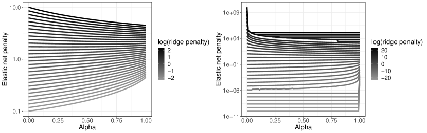
Figure 1: Transformed elastic net penalty for various $\alpha$ and ridge penalty.

2.3 Overlapping groups

So far, we have assumed the groups to be non-overlapping. A simple way to allow for partly overlapping groups is to make artifical, non-overlapping groups, similarly as proposed as naive implementation of the latent overlapping group lasso (Jacob et al., 2009).

First consider group-regularised ridge models, for which we define $\boldsymbol{\tau}=\phi\boldsymbol{\lambda}_{R}^{-1}$. We model the prior variance by the average over multiple groups, given in $Z\boldsymbol{\tau}$, as used in (van Nee et al., 2020). Let $\bar{X}$ denote the observed data matrix where each column $k$ of the original matrix $X$ is duplicated $I_{k}$ times for each of the $I_{k}$ groups covariate $k$ belongs to, with group indices given in $\mathcal{I}_{k}$. Let $\bar{X}^{\prime}$ denote the matrix where the columns are additionally scaled by $\frac{1}{\sqrt{I_{k}}}$. Define the extended vector of artificial regression coefficients by $\bar{\boldsymbol{\beta}}$ and the extended vector with scaled artificial regression coefficients by $\bar{\boldsymbol{\beta}}^{\prime}$. Each column duplicated from the original column $k$ now corresponds to an artificial, independent effect $\beta_{k_{g}}=\frac{1}{\sqrt{I_{k}}}\beta_{k_{g}}^{\prime}\overset{ind.}{\sim}N(0,\tau_{g}^{2}/I_{k})$ for $k=1,..,p,$ and $g\in\mathcal{I}_{k}$. The effect of a covariate $k$ is equal to the sum of the contributions of the groups, $\beta_{k}=\sum_{g\in\mathcal{I}_{k}}\beta_{k_{g}}=\frac{1}{\sqrt{I_{k}}}\sum_{g\in\mathcal{I}_{k}}\beta_{k_{g}}^{\prime}$, such that $X\boldsymbol{\beta}=\bar{X}\bar{\boldsymbol{\beta}}=\bar{X}^{\prime}\bar{\boldsymbol{\beta}}^{\prime}$. The prior distribution of $\beta_{k_{g}}^{\prime}$ is given by $N(0,\tau_{g}^{2})=N(0,\phi\lambda_{R,g})$. Hence, we can use our proposed method on the scaled, duplicated $\bar{X}^{\prime}$ to obtain the estimates for the prior parameters $\phi,\boldsymbol{\lambda}_{R}$. Finally, the variance estimates are pooled by the co-data matrix $Z$ to compute $\boldsymbol{\beta}$ with ridge prior variances $Z\phi\boldsymbol{\lambda}_{R}^{-1}$.

For elastic net models, we first transform the ridge prior variances given in $Z\phi\boldsymbol{\lambda}_{R}^{-1}$ to elastic net penalties as described above.

The high-dimension of $\bar{X}$ increases fast for largely overlapping groups. In practice, however, it is not necessary to store this matrix, nor will it increase the computational time as fast, as the computations for the marginal likelihood only require the high-dimensional computation of $G$ $n\times n$-dimensional matrices $\bar{X}^{\prime}_{g}\bar{X}^{\prime}_{g}{}^{T}$ once. Note that one should take care in including highly overlapping groups as this results in highly correlated groups.

2.4 Recalibration by cross-validation

In particular for non-linear models, like logistic regression, we experienced that the components $\lambda_{g}$ of $\boldsymbol{\lambda}$ were estimated well in a relative sense, but less so in the absolute sense. This may be due to the Laplace approximation of the likelihood, which is rather coarse for binary outcomes, while being exact for the linear model. Therefore, the predictive performance may benefit from using recalibrated group-penalties: $\boldsymbol{\lambda}^{\prime}=\lambda_{0}\boldsymbol{\lambda}$, where $\boldsymbol{\lambda}$ are the estimated penalty factors, and $\lambda_{0}$ is a global rescaling penalty. As $\lambda_{0}$ is a scalar, it is efficiently and easily estimated by cross-validation, e.g. by using glmnet with penalty factors $\boldsymbol{\lambda}$.

3 Data examples

The method is termed squeezy as it squeezes out some sparsity from dense group-adaptive ridge models. We conduct a model-based linear regression simulation study and illustrate the method on a cancer genomics example in the logistic regression setting. We include the following elastic net models to compare performance and computation time:

1. EN (glmnet, Friedman et al. (2010)): a co-data agnostic elastic net penalty, with global penalty parameter obtained by cross-validation;

2. fwEN and fwEN (continuous) (fwelnet, Tay et al. (2020)): a globally adaptive elastic net penalty on group level for grouped data (fwEN) or elastic net penalty with weights a function of continuous co-data (fwEN (continuous)). Note that we include fwelnet (continuous) only in the cancer genomics data example for which continuous co-data is available;

3. ipf and ipf2 (ipflasso, Boulesteix et al. (2017)): a group-adaptive elastic net penalty, with the group penalty factors selected from a grid of possible values. We take the grid where each penalty factor is in $\{1,2\}$ (ipf) or in $\{1,2,4\}$ (ipf2). Note that we only include the computationally expensive ipf2 in the model-based simulated data example for comparison of computing times;

4. gren (gren, Münch et al. (2019)): a group-adaptive elastic net penalty, with the group penalty factors obtained by an approximate empirical-variational Bayes framework. Note that gren is not included in the first linear regression example, as it is not implemented for the linear model;

5. ecpcEN squeezy (ecpc, van Nee et al. (2020) and squeezy): a group-adaptive elastic net penalty. The method ecpc provides empirical Bayes moment estimates for group-adaptive ridge penalties. We use squeezy to transform these to elastic net penalties combined with a recalibrated global rescaling penalty;

6. squeezy (single) and squeezy (single+reCV): a co-data agnostic elastic net penalty, where the global penalty is obtained by transforming the marginal likelihood estimate for the ridge penalty to an elastic net penalty, without or with recalibration of a global rescaling penalty. While glmnet internally standardises linear response, squeezy (single+reCV) does not;

7. squeezy (multi) and squeezy (multi+reCV): a group-adaptive elastic net penalty using the proposed method, without or with recalibration of a global rescaling penalty.

3.1 Model-based simulation study

We simulate training and test sets of observed data $X$ in $10$ correlated blocks of size $p/10$, regression coefficients from a Laplace distribution ($\alpha=1$) with mean zero and group-specific scale parameter $b_{g_{k}}$, $g_{k}\in\{1,..,5\}$, for $5$ equally sized groups, and response from a normal distribution:

$$\boldsymbol{x}_{i,b} \overset{ind.}{\sim}N\left(\boldsymbol{0},I_{(p/10)\times(p/10)}+\frac{\rho^{2}}{(1-\rho)^{2}}\boldsymbol{1}_{(p/10)\times(p/10)}\right),\ i=1,..,n,\ b=1,..,10,$$

$$\beta_{k} \overset{ind.}{\sim}Laplace(0,b_{k_{g}}),\ k=1,..,p,\ \boldsymbol{Y}\sim N(X\boldsymbol{\beta},\sigma^{2}I_{n\times n}),$$

with $\rho=0.2$ and $\sigma^{2}=2$. We consider three settings of group parameters: i) no groups: the group scale parameters $\boldsymbol{b}$ are the same and chosen such that the variance under each group prior is equal to $(0.1,0.1,0.1,0.1,0.1)\cdot\frac{1200}{p}$; ii) weakly informative groups: the group scale parameters are different, but less so than in the third setting. The variances match $(0.141,0.161,0.186,0.336,0.536)\cdot\frac{1200}{p}$; iii) informative groups: groups are different, with variances matching $(0.01,0.05,0.1,0.4,0.8)\cdot\frac{1200}{p}$.

First, we fit the methods listed above for $\alpha=0.3$ on $100$ independent training and test sets, with $n=150$, $p=600$ and the co-data providing group membership of the $G=5$ groups, to compare performance. Our method squeezy easily obtains optimal elastic net group penalties for a range of $\alpha$. We observe that there is usually little benefit from recalibration by cross-validation (reCV) in the linear case (Figure 2).

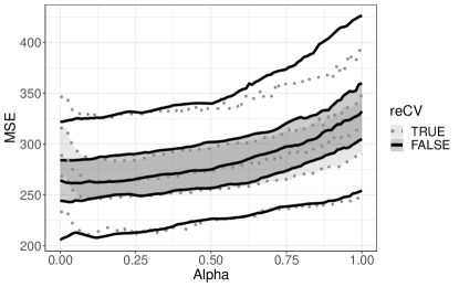
Figure 2: Model-based simulation study, informative groups setting. MSE performance of squeezy (multi) and squeezy (multi+reCV) on the test sets of $100$ pairs of training and test sets for $100$ evenly spaced values of $\alpha\in[0,1]$, shown in pointwise quantiles of $(0.05,0.25,0.5,0.75,0.95)$.

Figure 3 shows the MSE performance on the test sets for all methods. Our proposed method performs well. The method squeezy (single) (either with or without reCV) outperforms the other methods in the single group setting. The difference in performance between squeezy (single+reCV) and EN may be due to loss of information due to the internally standardisation of the linear response of EN. More importantly, squeezy (multi) (either with or without reCV) outperforms the other methods including squeezy (single) in the setting with informative groups, illustrating the benefit of informative co-data. The performance of squeezy (multi) and squeezy (single) is more alike in the setting with weakly informative groups, and superior to the other methods. The method performs better when maximum marginal likelihood estimates for ridge penalties are transformed (squeezy) than when moment estimates are transformed (ecpc EN squeezy). Note that the performance of ipf might improve by using a larger grid, but only at a very substantial computational cost as shown in Figure 4. While the difference in performance between squeezy and the other methods is smaller for $\alpha=0.8$, squeezy (multi) still outperforms the other methods when the co-data is informative (Figure B1 in Appendix B).

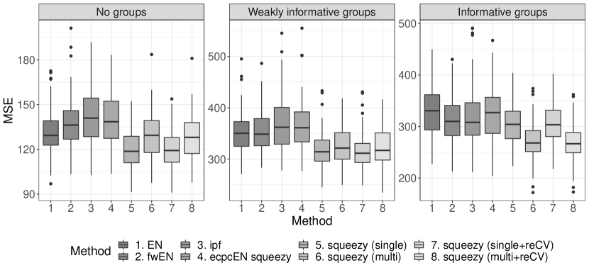
Figure 3: Model-based simulation study. Box plots of the MSE performance on the test sets of $100$ pairs of training and test sets, $\alpha=0.3$.

Then, we fit the methods on $5$ training sets to compare computation time for varying $n$, $p$ and $G$. The group parameters are set according to the setting with informative groups. We set $(n,p,G)=(150,1200,5)$. Then we vary one of $n,p,G$ while keeping the others fixed. Figure 4 shows the average computation time for fitting the models. Unsurprisingly, the group-adaptive methods are slower than the other methods, but squeezy scales substantially better than ipf in the number of groups.

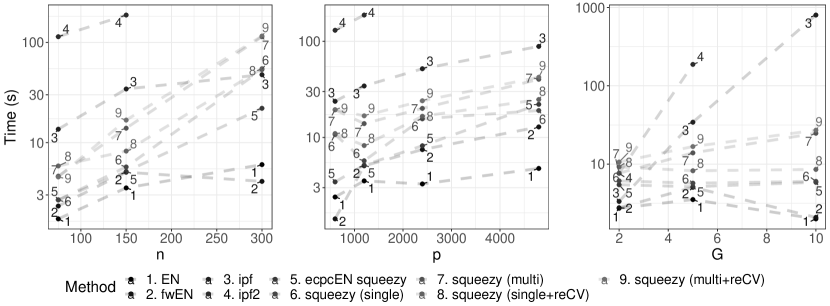
Figure 4: Model-based simulation study. Average computation time in $5$ training sets for varying $n$, $p$ and $G$.

3.2 Application to predicting therapy response

We apply squeezy to predict therapy response (clinical benefit versus progressed disease) using microRNA (miRNA) data from a study on colorectal cancer (Neerincx et al., 2018), consisting of $p=2114$ miRNA expression levels for $n=88$ independent individuals. As co-data, we use false discovery rates (FDRs) for differential expression in the primary tumour versus adjacent colorectal tissue. The FDRs were obtained in a previous study (Neerincx et al., 2015) from a different set of non-overlapping samples. These co-data were previously shown to be informative for the prediction, miRNAs that are tumor-specific tend to be more important for the response prediction (van Nee et al., 2020). Here, we discretise the continuous FDRs in $G=8$ equally sized groups, such that we have around $10$ samples per group parameter.

We fit the methods listed above on $10$ folds to compare cross-validated performance (Figure 5) and average computation time (Table 1). Figure 5 (left) clearly shows the benefit of recalibration by cross-validation (reCV) in this logistic regression setting. Our method squeezy (multi+reCV) performs as well as gren (Figure 5 (right), cf 10 vs 5) but is around 35 times as fast. The method ecpcEN squeezy is twice as fast as squeezy (multi+reCV) and is competitive to squeezy (multi+reCV) and gren. These three methods all benefit from the informative co-data and outperform the other methods.

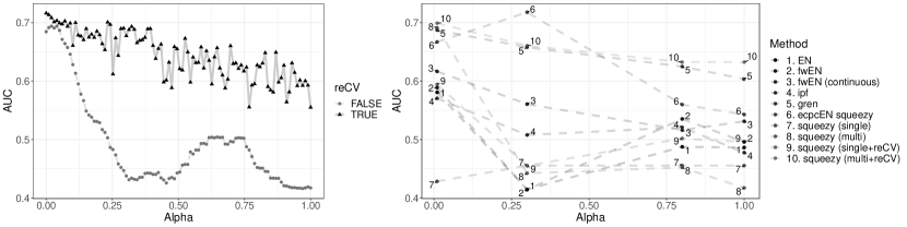
Figure 5: Results of 10-fold cross-validation in miRNA data example. Left: AUC performance for squeezy (multi) and squeezy (multi+reCV) for $100$ evenly spaced values of $\alpha\in[0,1]$. Right: AUC performance for several values of $\alpha$ for various methods.

Method	Time (s)	Method	Time (s)
1. EN	1.17 (1.06)	2. fwEN (groups)	12.20 (6.84)
7. squeezy (single)	5.12 (3.29)	10. squeezy (multi+reCV)	13.58 (13.59)
6. ecpcEN squeezy	5.48 (3.01)	3. fwEN (continuous)	14.11 (11.13)
9. squeezy (single+reCV)	7.45 (5.77)	5. gren	351.52 (96.74)
8. squeezy (multi)	10.47 (10.50)	4. ipf	422.39 (259.80)

Table 1: Results of 10-fold CV in miRNA data example. Mean time per fold and standard deviation over folds, sorted from shortest to longest time.

4 Discussion

The proposed method, termed squeezy, computes fast marginal likelihood estimates for group-adaptive elastic net penalties. The method estimates those penalties by deducing them from group-adaptive ridge penalties, for which we derive a low-dimensional representation of the Taylor approximation of the marginal likelihood and its first derivative for generalised linear models, using results from (Wood, 2011). Squeezy implements this and uses Nelder-Mead optimisation to find the penalties. An extension would be to also use the hessian (Wood, 2011), which may speed up the optimisation.

An alternative implementation of our method uses the R-package mgcv (Wood, 2011) to estimate the ridge penalties from the linear predictors, as detailed in (van de Wiel et al., 2020). As mgcv does not allow for more variables than samples, this solution cannot include unpenalised variables. A fix to this is to include these as pre-estimated offsets. In the absence of unpenalised variables, we found that the two implementations provided similar results at comparable computing times. The alternative solution opens up for application of squeezy to a wider variety of models (provided that the elastic net counter part is also available) such as the penalised Cox model for survival data.

We showed that the marginal likelihood of ridge models also approximates the marginal likelihood of elastic net models, by using the asymptotic multivariate normality of the linear predictor. This result also holds for other priors with finite variance. When co-data includes many groups, for example, a hierarchical prior could be used for shrinkage or selection on group level. The result does not hold for priors with infinite variance, such as the highly sparse horseshoe prior (Carvalho et al., 2009). Moreover, the practical use of our method for other relatively sparse priors should be tested.

The method transforms the ridge penalties to elastic net penalties using the variance function of the elastic net prior. We showed in a data example that it is beneficial to recalibrate the transformed elastic net penalties in logistic regression. Furthermore, the simulation study and data example showed that our method is more scalable and faster than other group-adaptive methods, while it benefits from co-data and performs as well as or better than other (group-adaptive) methods.

Should squeezy perform inferior to other methods, it may be useful to check whether this might be due to invalidity of the multivariate normal assumption for $\boldsymbol{\eta}=X\boldsymbol{\beta}$. Once the elastic net prior(s) for $\boldsymbol{\beta}$ are known, it is straightforward to generate multiple $\boldsymbol{\eta}$ realisations. Then, we suggest using those to generate a chi-square-based Q-Q plot, e.g. by the R-package MVN (Korkmaz et al., 2014), to verify multivariate normality.

As our method is based on (marginal) likelihood, it in principle facilitates model selection in terms of the hyper-parameters (e.g. single group versus multi-group) by the use of information criteria (Greven and Kneib, 2010). To what extent which criterion is useful in our setting is a topic for further research.

We provide the R-package squeezy and scripts demonstrating the package and reproducing the results on https://github.com/Mirrelijn/squeezy.

Appendix

A Details for Laplace approximate marginal likelihood for group-adaptive ridge models

We provide details of the derivation of a low-dimensional representation of the Laplace approximation for the marginal likelihood and its first derivative as stated in Equations (6) and (8). When some covariates are left unpenalised, we need to integrate over the penalised covariates only. Wood (2011) forms an ortogonal basis $U$ for the range space of $S$. For group-adaptive ridge penalties, this orthogonal basis is simply given by the identity matrix, as $S$ is diagonal with zeros for unpenalised covariates. The proposed reparametrisation of $X$ and $S$ boils down to simply taking the columns in $X$ that correspond to the penalised variables, $\bar{X}=X_{pen}$, and taking the columns and rows of the penalty matrix that correspond to the penalised variables, $\bar{S}=S_{pen}=\Lambda_{pen}=\sum_{g}\lambda_{g}S_{g,pen}$.

A.1 Laplace approximate marginal likelihood

The high-dimensional log-marginal likelihood approximation is given in Equation (5) in (Wood, 2011) and may be written as:

$$]-\ell(\boldsymbol{\lambda}) \approx\frac{D_{p}}{2\phi}-\ell_{s}(\phi)+\frac{\log(\bar{X}^{T}W\bar{X}+\bar{S})-\log(|S|_{+})}{2}$$

$$=-\ell(\hat{\boldsymbol{\beta}})+\frac{1}{2\phi}\hat{\boldsymbol{\beta}}^{T}\Lambda_{pen}\hat{\boldsymbol{\beta}}+\frac{1}{2}\log(|X_{pen}^{T}WX_{pen}+\Lambda_{pen}|)-\frac{1}{2}\log(|\Lambda_{pen}|).$$ (A1)

When we use Newton iterations to obtain $\hat{\boldsymbol{\beta}}$ or $\hat{\boldsymbol{\eta}}$, upon convergence:

$$\hat{\boldsymbol{\beta}}=(X^{T}WX+\Lambda)^{-1}X^{T}(\boldsymbol{y}-\boldsymbol{\mu}+WX\hat{\boldsymbol{\beta}}),$$

$$\hat{\boldsymbol{\eta}}=X(X^{T}WX+\Lambda)^{-1}X^{T}(\boldsymbol{y}-\boldsymbol{\mu}+W\hat{\boldsymbol{\eta}}).$$

We substitute this in the second term of the log-marginal likelihood approximation:

$$\hat{\boldsymbol{\beta}}^{T}\Lambda\hat{\boldsymbol{\beta}} =(\boldsymbol{y}-\boldsymbol{\mu}+WX\hat{\boldsymbol{\beta}})^{T}X(X^{T}WX+\Lambda)^{-1}\Lambda\hat{\boldsymbol{\beta}}$$

$$=(\boldsymbol{y}-\boldsymbol{\mu}+WX\hat{\boldsymbol{\beta}})^{T}X(I_{p\times p}-(X^{T}WX+\Lambda)^{-1}X^{T}WX)\hat{\boldsymbol{\beta}}$$

$$=(\boldsymbol{y}-\boldsymbol{\mu}+WX\hat{\boldsymbol{\beta}})^{T}\hat{\boldsymbol{\eta}}-\hat{\boldsymbol{\eta}}^{T}W\hat{\boldsymbol{\eta}}$$

$$=(\boldsymbol{y}-\boldsymbol{\mu})^{T}\hat{\boldsymbol{\eta}}.$$

The latter two terms may be rewritten in a lower-dimensional representation by:

$$\frac{1}{2}\log(|X_{pen}^{T}WX_{pen}+\Lambda_{pen}|)-\frac{1}{2}\log(|\Lambda_{pen}|)=-\frac{1}{2}\log(|(X_{pen}^{T}WX_{pen}+\Lambda_{pen})^{-1}\Lambda_{pen}|)$$

$$=-\frac{1}{2}\log(|I_{pen\times pen}-(X_{pen}^{T}WX_{pen}+\Lambda_{pen})^{-1}X_{pen}^{T}WX_{pen}|)$$

$$=-\frac{1}{2}\log(|I_{n\times n}-WX_{pen}(X_{pen}^{T}WX_{pen}+\Lambda_{pen})^{-1}X_{pen}^{T}|)$$

$$=-\frac{1}{2}\log(|I_{n\times n}-WH_{pen}|),$$

where efficient representations for $H_{pen}$ exist (van de Wiel et al., 2020).

So, the low-dimensional Laplace approximation for the minus log-marginal likelihood is:

$$-\ell(\boldsymbol{\lambda}) \approx-\ell(\hat{\boldsymbol{\eta}})+\frac{1}{2\phi}(\boldsymbol{y}-\boldsymbol{\mu})^{T}\hat{\boldsymbol{\eta}}-\frac{1}{2}\log(|I_{n\times n}-WH_{pen}|).$$

A.2 First derivative of Laplace approximate marginal likelihood

We derive low-dimensional representations of the derivatives to $\rho_{g}=\log(\lambda_{g})$ for $g=1,..,G$, as derived in a high-dimensional representation by (Wood, 2011).

A.2.1 Derivative of $\frac{\partial\hat{\boldsymbol{\eta}}}{\partial\rho_{g}}$

Denote by $I_{g}\in\mathbb{R}^{p\times p}$ the diagonal matrix with diagonal element $k$ equal to $1$ if $k$ is in group $g$ and $0$ otherwise and define $\Lambda_{g}=\lambda_{g}I_{g}$. The derivative for $\hat{\boldsymbol{\beta}}$ is then given by (Wood, 2011):

$$\frac{\partial\hat{\boldsymbol{\beta}}}{\partial\rho_{g}} =-\exp(\rho_{g})(X^{T}WX+S)^{-1}S_{g}\hat{\boldsymbol{\beta}}$$

$$=-\exp(\rho_{g})(X^{T}WX+\Lambda)^{-1}\Lambda_{g}\frac{1}{\lambda_{g}}\hat{\boldsymbol{\beta}}$$

$$=-\exp(\rho_{g})(X^{T}WX+\Lambda)^{-1}\Lambda\frac{1}{\lambda_{g}}I_{g}\hat{\boldsymbol{\beta}}$$

$$=-\exp(\rho_{g})\left[I_{p\times p}-(X^{T}WX+\Lambda)^{-1}X^{T}WX\right]\frac{1}{\lambda_{g}}I_{g}\hat{\boldsymbol{\beta}}$$

$$=-\exp(\rho_{g})\left[I_{p\times p}-(X^{T}WX+\Lambda)^{-1}X^{T}WX\right]\frac{1}{\lambda_{g}}I_{g}(X^{T}WX+\Lambda)^{-1}X^{T}\left(\boldsymbol{y}-\boldsymbol{\mu}+W\hat{\boldsymbol{\eta}}\right).$$

We can write the derivative for $\hat{\boldsymbol{\eta}}$ as:

$$\frac{\partial\hat{\boldsymbol{\eta}}}{\partial\rho_{g}} =X\frac{\partial\hat{\boldsymbol{\beta}}}{\partial\rho_{g}}$$

$$=-\exp(\rho_{g})X\left[I_{p\times p}-(X^{T}WX+\Lambda)^{-1}X^{T}WX\right]\frac{1}{\lambda_{g}}I_{g}(X^{T}WX+\Lambda)^{-1}X^{T}\left(\boldsymbol{y}-\boldsymbol{\mu}+W\hat{\boldsymbol{\eta}}\right)$$

$$=-\exp(\rho_{g})\left[I_{n\times n}-X(X^{T}WX+\Lambda)^{-1}X^{T}W\right]X\frac{1}{\lambda_{g}}I_{g}(X^{T}WX+\Lambda)^{-1}X^{T}\left(\boldsymbol{y}-\boldsymbol{\mu}+W\hat{\boldsymbol{\eta}}\right)$$

$$=-\exp(\rho_{g})\left[I_{n\times n}-HW\right]\frac{1}{\lambda_{g}}H_{g}^{T}\left(\boldsymbol{y}-\boldsymbol{\mu}+W\hat{\boldsymbol{\eta}}\right),$$

with $H_{g}$, which can be seen as a contribution of the $g^{th}$ group to the hat matrix, defined as:

$$\begin{split}&H_{g}:=X(X^{T}WX+\Lambda)^{-1}I_{g}X^{T}=W^{-\frac{1}{2}}P_{1}W^{\frac{1}{2}}\left(I_{n\times n}-X_{pen}\Lambda^{-1}_{pen}X_{pen}^{T}W^{\frac{1}{2}}P_{1}W^{-\frac{1}{2}}\right.\\ &\qquad\cdot\left.[W^{-1}+X_{pen}\Lambda^{-1}X_{pen}^{T}W^{\frac{1}{2}}P_{1}W^{-\frac{1}{2}}]^{-1}\right)\lambda_{g}^{-1}X_{g}X_{g}^{T},\end{split}$$

where we have used (van de Wiel et al., 2020):

$$P_{1}=I_{n\times n}-W^{\frac{1}{2}}X_{unpen}(X_{unpen}^{T}WX_{unpen})^{-1}X_{unpen}^{T}W^{\frac{1}{2}},$$

$$\begin{split}&[X(X^{T}WX+\Lambda)^{-1}]_{pen}=W^{-\frac{1}{2}}P_{1}W^{\frac{1}{2}}\left(X_{pen}\Lambda^{-1}_{pen}-X_{pen}\Lambda^{-1}_{pen}X_{pen}^{T}W^{\frac{1}{2}}P_{1}W^{-\frac{1}{2}}\right.\\ &\qquad\cdot\left.[W^{-1}+X_{pen}\Lambda^{-1}X_{pen}^{T}W^{\frac{1}{2}}P_{1}W^{-\frac{1}{2}}]^{-1}X_{pen}\Lambda_{pen}^{-1}\right).\end{split}$$

A.2.2 Derivative of $\frac{\partial\ell(\hat{\boldsymbol{\eta}})}{\partial\rho_{g}}$

Wood (2008) derives partials for the deviance of generalised linear models:

$$\frac{\partial\ell(\hat{\boldsymbol{\beta}})}{\partial\hat{\boldsymbol{\beta}}} =\frac{1}{\phi}X^{T}\frac{\boldsymbol{y}-\boldsymbol{\mu}}{V(\boldsymbol{\mu})\odot g^{\prime}(\boldsymbol{\mu})},$$

where division by $V(\boldsymbol{\mu})\odot g^{\prime}(\boldsymbol{\mu})$ is element-wise and $\odot$ representing element-wise multiplication. The derivative of the log likelihood is then given by:

$$\frac{\partial\ell(\hat{\boldsymbol{\eta}})}{\partial\rho_{g}}=\frac{\partial\ell(\hat{\boldsymbol{\beta}})}{\partial\rho_{g}} =\frac{\partial\ell(\hat{\boldsymbol{\beta}})}{\partial\hat{\boldsymbol{\beta}}}^{T}\frac{\partial\hat{\boldsymbol{\beta}}}{\partial\rho_{g}}$$

$$=-\exp(\rho_{g})\frac{1}{\phi}\left(\frac{\boldsymbol{y}-\boldsymbol{\mu}}{V(\boldsymbol{\mu})}\right)^{T}G^{\prime-1}X(X^{T}WX+\Lambda)^{-1}\Lambda_{g}\frac{1}{\lambda_{g}}\hat{\boldsymbol{\beta}}$$

$$=-\exp(\rho_{g})\frac{1}{\phi}\left(\frac{\boldsymbol{y}-\boldsymbol{\mu}}{V(\boldsymbol{\mu})}\right)^{T}G^{\prime-1}\left[I_{n\times n}-HW\right]\frac{1}{\lambda_{g}}H_{g}^{T}\left(\boldsymbol{y}-\boldsymbol{\mu}+W\hat{\boldsymbol{\eta}}\right),$$

with $G^{\prime}$ a diagonal matrix with diagonal elements $g^{\prime}(\mu_{i})$.

A.2.3 Derivative of $\frac{1}{2\phi}(\boldsymbol{y}-\boldsymbol{\mu})^{T}\hat{\boldsymbol{\eta}}$

We have for the low-dimensional penalty term, recall that $\boldsymbol{\mu}=g^{-1}(\boldsymbol{\eta})$:

$$\frac{\partial}{\partial\rho_{g}}\left(\frac{1}{2\phi}(\boldsymbol{y}-\boldsymbol{\mu})^{T}\hat{\boldsymbol{\eta}}\right) =\frac{1}{2\phi}\left(\frac{\partial(\boldsymbol{y}-\boldsymbol{\mu})^{T}}{\partial\rho_{g}}\hat{\boldsymbol{\eta}}+(\boldsymbol{y}-\boldsymbol{\mu})^{T}\frac{\partial\hat{\boldsymbol{\eta}}}{\partial\rho_{g}}\right)$$

$$=\frac{1}{2\phi}\left(\frac{\partial(-\boldsymbol{\mu}^{T})}{\partial\rho_{g}}\hat{\boldsymbol{\eta}}+(\boldsymbol{y}-\boldsymbol{\mu})^{T}\frac{\partial\hat{\boldsymbol{\eta}}}{\partial\rho_{g}}\right)$$

$$=\frac{1}{2\phi}\left(-\frac{\partial\hat{\boldsymbol{\eta}}^{T}}{\partial\rho_{g}}G^{\prime-1}\hat{\boldsymbol{\eta}}+(\boldsymbol{y}-\boldsymbol{\mu})^{T}\frac{\partial\hat{\boldsymbol{\eta}}}{\partial\rho_{g}}\right)$$

$$=\frac{1}{2\phi}\left(-G^{\prime-1}\hat{\boldsymbol{\eta}}+\boldsymbol{y}-\boldsymbol{\mu}\right)^{T}\frac{\partial\hat{\boldsymbol{\eta}}}{\partial\rho_{g}}$$

$$=-\exp(\rho_{g})\frac{1}{2\phi}\left(-G^{\prime-1}\hat{\boldsymbol{\eta}}+\boldsymbol{y}-\boldsymbol{\mu}\right)^{T}\left[I_{n\times n}-HW\right]\frac{1}{\lambda_{g}}H_{g}^{T}\left(\boldsymbol{y}-\boldsymbol{\mu}+W\hat{\boldsymbol{\eta}}\right).$$

A.2.4 Derivative of $-\frac{1}{2}\log(|\boldsymbol{I}_{n\times n}-\boldsymbol{W}\boldsymbol{H}_{pen}|)$

We have for the third term in Equation (A.1):

$$\frac{\partial}{\partial\rho_{g}}\left(\frac{1}{2}\log(|X_{pen}^{T}WX_{pen}+\Lambda_{pen}|\right) =\frac{1}{2}tr\left((X_{pen}^{T}WX_{pen}+\Lambda_{pen})^{-1}\frac{\partial X_{pen}^{T}WX_{pen}+\Lambda_{pen}}{\partial\rho_{g}}\right)$$

$$=\frac{1}{2}tr\left((X_{pen}^{T}WX_{pen}+\Lambda_{pen})^{-1}X_{pen}^{T}\frac{\partial W}{\partial\rho_{g}}X_{pen}\right)$$

$$\qquad+\frac{1}{2}tr\left((X_{pen}^{T}WX_{pen}+\Lambda_{pen})^{-1}\Lambda_{g}\right)$$

$$=\frac{1}{2}tr\left(X_{pen}(X_{pen}^{T}WX_{pen}+\Lambda_{pen})^{-1}X_{pen}^{T}\frac{\partial W}{\partial\rho_{g}}\right)$$

$$\qquad+\frac{1}{2}tr\left((X_{pen}^{T}WX_{pen}+\Lambda_{pen})^{-1}\Lambda_{g}\right)$$

$$=\frac{1}{2}tr\left(H_{pen}\frac{\partial W}{\partial\rho_{g}}\right)+\frac{1}{2}tr(I_{g})$$

$$\qquad-\frac{1}{2}tr\left(\Lambda_{pen}^{-1}X_{pen}^{T}(W^{-1}+X_{pen}\Lambda_{pen}^{-1}X_{pen}^{T})^{-1}X_{pen}I_{g}\right)$$

$$=\frac{1}{2}tr\left(H_{pen}\frac{\partial W}{\partial\rho_{g}}\right)+\frac{1}{2}tr(I_{g})$$

$$\qquad-\frac{1}{2}tr\left(\lambda_{g}^{-1}X_{g}X_{g}^{T}(W^{-1}+X_{pen}\Lambda_{pen}^{-1}X_{pen}^{T})^{-1}\right),$$

where we have used the following equalities:

$$(X_{pen}^{T}WX_{pen}+\Lambda_{pen})^{-1} =\Lambda_{pen}^{-1}-\Lambda_{pen}^{-1}X_{pen}^{T}(W^{-1}+X_{pen}\Lambda_{pen}^{-1}X_{pen}^{T})^{-1}X_{pen}\Lambda_{pen}^{-1}$$

$$H_{pen} =X_{pen}(X_{pen}^{T}WX_{pen}+\Lambda_{pen})^{-1}X_{pen}^{T},$$

with the partials of $W\in\mathbb{R}^{n\times n}$ readily obtained from (Wood, 2011).

For the latter term in Equation (A.1):

$$\frac{\partial}{\partial\rho_{g}}\left(-\frac{1}{2}\log(|\Lambda_{pen}|)\right) =-\frac{1}{2}tr\left(\Lambda_{pen}^{-1}\frac{\partial\Lambda_{pen}}{\partial\rho_{g}}\right)$$

$$=-\frac{1}{2}tr\left(\Lambda_{pen}^{-1}I_{g}\frac{\partial\lambda_{g}}{\partial\rho_{g}}\right)$$

$$=-\frac{1}{2}tr(I_{g})\frac{1}{\lambda_{g}}\lambda_{g}$$

$$=-\frac{1}{2}tr(I_{g}).$$

So, the derivative of the Laplace approximate minus log marginal likelihood is given by:

$$\frac{\partial-\ell(\boldsymbol{\rho})}{\partial\rho_{g}} =\frac{1}{\phi}\left(\frac{\boldsymbol{y}-\boldsymbol{\mu}}{V(\boldsymbol{\mu})}\right)^{T}G^{\prime-1}\left[I_{n\times n}-HW\right]H_{g}^{T}\left(\boldsymbol{y}-\boldsymbol{\mu}+W\hat{\boldsymbol{\eta}}\right)$$

$$\qquad-\frac{1}{2\phi}\left(-G^{\prime-1}\hat{\boldsymbol{\eta}}+\boldsymbol{y}-\boldsymbol{\mu}\right)^{T}\left[I_{n\times n}-HW\right]H_{g}^{T}\left(\boldsymbol{y}-\boldsymbol{\mu}+W\hat{\boldsymbol{\eta}}\right)$$

$$\qquad+\frac{1}{2}tr\left(H_{pen}\frac{\partial W}{\partial\rho_{g}}\right)-\frac{1}{2}tr\left(\lambda_{g}^{-1}X_{g}X_{g}^{T}(W^{-1}+X_{pen}\Lambda_{pen}^{-1}X_{pen}^{T})^{-1}\right).$$

A.3 Details for linear regression

Denote by $\phi(\cdot;\mu,\sigma^{2})$ the normal pdf with mean $\mu$ and variance $\sigma^{2}$. The Laplace approximation is in fact exact for linear regression. We need the following parameters:

$$\phi =\sigma^{2},V(\mu)=1,\ell(\hat{\boldsymbol{\eta}})=\sum_{i=1}^{n}\log(\phi(y_{i};\hat{\boldsymbol{\eta}}_{i},\sigma^{2})),$$

$$\boldsymbol{\mu} =\hat{\boldsymbol{\eta}},\ W=I_{n\times n},\ g(\mu)=\mu,\ g^{\prime}(\mu)=1,\ G^{\prime-1}=I_{n\times n}.$$

The partial derivative of the minus log likelihood to the scale parameter $\phi=\sigma^{2}$ from Equation (9) is given by:

$$\frac{\partial-\ell(\hat{\boldsymbol{\eta}},\sigma^{2})}{\partial\sigma^{2}} =\frac{n}{2\sigma^{2}}-\frac{1}{2\sigma^{4}}(\boldsymbol{y}-\hat{\boldsymbol{\eta}})^{T}(\boldsymbol{y}-\hat{\boldsymbol{\eta}}).$$

A.4 Details for logistic regression

We need the following parameters:

$$\phi =1,V(\mu_{i})=\mu_{i}(1-\mu_{i}),\ell(\hat{\boldsymbol{\eta}})=\sum_{i=1}^{n}y_{i}\log(expit(\hat{\eta}_{i}))+(1-y_{i})\log(1-expit(\hat{\eta}_{i})),$$

$$\boldsymbol{\mu} =expit(\hat{\boldsymbol{\eta}})=(1+\exp(-\hat{\boldsymbol{\eta}}))^{-1},$$

$$W =diag(\boldsymbol{\mu}\odot(1-\boldsymbol{\mu})),\ \alpha_{i}=1,\ \frac{\partial w_{i}}{\partial\eta_{i}}=\mu_{i}(1-\mu_{i})(2\mu_{i}-1),$$

$$g(\mu_{i}) =logit(\mu_{i}),\ g^{\prime}(\mu_{i})=(\mu_{i}(1-\mu_{i}))^{-1},\ G^{\prime-1}=W,\ g^{\prime\prime}(\mu_{i})=\frac{2\mu_{i}-1}{\mu_{i}^{2}(1-\mu_{i})^{2}}.$$

B Additional figures to the data examples

Figure B1 shows the MSE performance in the model-based simulation study for $\alpha=0.8$.

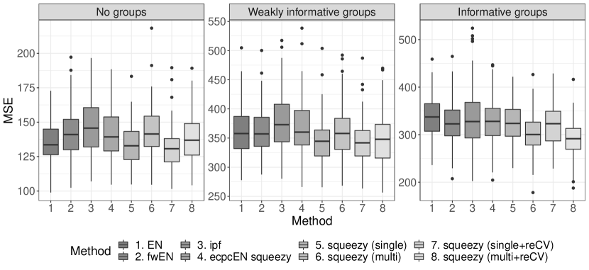
Figure B1: Model-based simulation study. Box plots of the MSE performance on the test sets of $50$ pairs of training and test sets, $\alpha=0.8$.

References

- Boulesteix et al. (2017) Anne-Laure Boulesteix, Riccardo De Bin, Xiaoyu Jiang, and Mathias Fuchs. Ipf-lasso: Integrative-penalized regression with penalty factors for prediction based on multi-omics data. Computational and mathematical methods in medicine, 2017, 2017.
- Carvalho et al. (2009) Carlos M Carvalho, Nicholas G Polson, and James G Scott. Handling sparsity via the horseshoe. In Artificial Intelligence and Statistics, pages 73–80. AISTATS, 2009.
- Eicker (1966) F Eicker. A multivariate central limit theorem for random linear vector forms. The Annals of Mathematical Statistics, pages 1825–1828, 1966.
- Friedman et al. (2010) Jerome Friedman, Trevor Hastie, and Rob Tibshirani. Regularization paths for generalized linear models via coordinate descent. Journal of statistical software, 33(1):1, 2010.
- Greven and Kneib (2010) Sonja Greven and Thomas Kneib. On the behaviour of marginal and conditional aic in linear mixed models. Biometrika, 97(4):773–789, 2010.
- Jacob et al. (2009) Laurent Jacob, Guillaume Obozinski, and Jean-Philippe Vert. Group lasso with overlap and graph lasso. In Proceedings of the 26th annual international conference on machine learning, pages 433–440. ACM, 2009.
- Korkmaz et al. (2014) Selcuk Korkmaz, Dincer Goksuluk, and Gokmen Zararsiz. Mvn: An r package for assessing multivariate normality. The R Journal, 6(2):151–162, 2014.
- Meier et al. (2008) L. Meier, S. van de Geer, and P. Bühlmann. The group Lasso for logistic regression. J. R. Stat. Soc. Ser. B Stat. Methodol., 70(1):53–71, 2008. ISSN 1369-7412.
- Münch et al. (2019) Magnus M Münch, Carel FW Peeters, Aad W van der Vaart, and Mark A van de Wiel. Adaptive group-regularized logistic elastic net regression. Biostatistics, 12 2019. ISSN 1465-4644. doi: 10.1093/biostatistics/kxz062. kxz062.
- Neerincx et al. (2015) Maarten Neerincx, DLS Sie, MA Van De Wiel, NCT Van Grieken, JD Burggraaf, H Dekker, PP Eijk, Bauke Ylstra, C Verhoef, GA Meijer, et al. Mir expression profiles of paired primary colorectal cancer and metastases by next-generation sequencing. Oncogenesis, 4(10):e170, 2015.
- Neerincx et al. (2018) Maarten Neerincx, Dennis Poel, Daoud LS Sie, Nicole CT van Grieken, Ram C Shankaraiah, Floor SW Van Der Wolf-De, Jan-Hein TM van Waesberghe, Jan-Dirk Burggraaf, Paul P Eijk, Cornelis Verhoef, et al. Combination of a six microrna expression profile with four clinicopathological factors for response prediction of systemic treatment in patients with advanced colorectal cancer. PloS one, 13(8):e0201809, 2018.
- Tay et al. (2020) J Kenneth Tay, Nima Aghaeepour, Trevor Hastie, and Robert Tibshirani. Feature-weighted elastic net: using” features of features” for better prediction. arXiv preprint arXiv:2006.01395, 2020.
- Tomczak et al. (2015) Katarzyna Tomczak, Patrycja Czerwińska, and Maciej Wiznerowicz. The cancer genome atlas (tcga): an immeasurable source of knowledge. Contemporary oncology, 19(1A):A68, 2015.
- van de Wiel et al. (2019) Mark A van de Wiel, Dennis E Te Beest, and Magnus M Münch. Learning from a lot: Empirical bayes for high-dimensional model-based prediction. Scandinavian Journal of Statistics, 46(1):2–25, 2019.
- van de Wiel et al. (2020) Mark A van de Wiel, Mirrelijn M van Nee, and Armin Rauschenberger. Fast cross-validation for multi-penalty ridge regression. arXiv preprint arXiv:2005.09301, 2020.
- van Nee et al. (2020) Mirrelijn M van Nee, Lodewyk FA Wessels, and Mark A van de Wiel. Flexible co-data learning for high-dimensional prediction. arXiv preprint arXiv:2005.04010, 2020.
- Veerman et al. (2019) Jurre R Veerman, Gwenaël GR Leday, and Mark A van de Wiel. Estimation of variance components, heritability and the ridge penalty in high-dimensional generalized linear models. Communications in Statistics-Simulation and Computation, pages 1–19, 2019.
- Wood (2008) Simon N Wood. Fast stable direct fitting and smoothness selection for generalized additive models. Journal of the Royal Statistical Society: Series B (Statistical Methodology), 70(3):495–518, 2008.
- Wood (2011) Simon N Wood. Fast stable restricted maximum likelihood and marginal likelihood estimation of semiparametric generalized linear models. Journal of the Royal Statistical Society: Series B (Statistical Methodology), 73(1):3–36, 2011.
- Zou and Hastie (2005) Hui Zou and Trevor Hastie. Regularization and variable selection via the elastic net. Journal of the Royal Statistical Society: Series B (Statistical Methodology), 67(2):301–320, 2005.