The Pauli Exclusion Operator: example of Hooke’s atom

Abstract

The Pauli Exclusion Operator (PEO) which ensures proper symmetry of the eigenstates of multi-electron systems with respect to exchange of each pair of electrons is introduced. Once PEO is added to the Hamiltonian, no additional constraints on multi-electron wave function due to the Pauli exclusion principle are needed. For two-electron states in two dimensions ($2D$) the PEO can be expressed in a closed form in terms of momentum operators, while in the position representation PEO is a non-local operator. Generalizations of PEO for multi-electron systems is introduced. Several approximations to PEO are discussed. Examples of analytical and numerical calculations of PEO are given for isotropic and anisotropic Hooke’s atom in $2D$. Application of approximate and kernel forms of PEO for calculations of energies and states in $2D$ Hooke’s atom are analyzed. Relation of PEO to standard variational calculations with the use of Slater determinant is discussed.

I Introduction

Two-electron systems, e.g. the helium atom, were analyzed from the early years of quantum mechanics Kellner1927 ; Hylleraas1928 ; Hylleraas1929 . Since the exact solutions of such situations are not known one usually calculates the energies of low states and the corresponding wave functions using the variational method. To be consisted with the Pauli exclusion principle Pauli1925 ; Pauli1940 one first selects the spin state of the electron pair, that is either a singlet or a triplet, and then assumes the trial functions of two electrons to be either symmetric or antisymmetric with respect to exchange of the two particles. This approach was successfully applied to the ground energy of the helium atom as well as to its excited states BetheBook ; Tanner2000 .

The Pauli exclusion principle can be introduced to the variational calculations by choosing the trial function of required symmetry with respect to exchange of the electrons. This approach may not be used in a numerical integration of the Schrodinger equation of the two electron systems since this equation does not include terms which can be related to the Pauli exclusion principle. Then, if one integrates this equation for two electrons or for two non-fermions having the same charges and masses as the electrons, then in both cases one obtains the same energies and states.

However, for the two-electron case some calculated states do not fulfill the Pauli exclusion principle and such states have to be eliminated as nonphysical ones. As an example, wave functions symmetric with respect to exchange of electrons are allowed for the singlet, but have to be eliminated for the triplet.

One can then state that, beyond the external potential and the Coulomb repulsion, there exists an additional spin-dependent field acting on both electrons which eliminates some states from the spectrum of the Hamiltonian $\hat{H}$. The presence of this field can be included in the model by introducing a spin-depended operator $\hat{P}$ responsible for the existence of the Pauli exclusion principle. The final effect of the operators $\hat{H}$ and $\hat{P}$ acting on the eigenstate $|\Psi(1,2)\rangle$ of $\hat{H}$ is that the states of the proper electron exchange symmetry are not altered but those of the improper symmetry vanish. Then, by solving numerically the Schrodinger equation with the operator $\left(\hat{H}-\hat{P}\right)$ instead of $\hat{H}$

$$\left(\hat{H}-\hat{P}\right)|\Psi(1,2)\rangle=E|\Psi(1,2)\rangle,$$ (1)

one automatically obtains states fulfilling the Pauli exclusion principle, and no additional constrains on multi-electron wave function due to the Pauli exclusion principle are needed. The main purpose of this work is to analyze the operator $\hat{P}$, [called further the Pauli Exclusion Operator (PEO)], in several two-electron systems. We show that in these cases it is possible to obtain PEO in a closed form. We also discuss generalization of PEO for multi-electron case and propose several approximations of this operator. Note that PEO exists in the literature in a different meaning and it was used to calculate nuclear matter Cheon1989 ; Schiller1999 ; Suzuki2000 , see Discussion.

It is impossible to obtain PEO for the helium atom because of two reasons. First, the Schrodinger equation of the latter does not separate into a sum of two one-electron equations, so one has to solve numerically the eigenequation in the six-dimensional space. Second, in the presence of the attractive Coulomb potential of helium nucleus there exist both localized and delocalized electron states, and the latter are difficult to be treated numerically.

There exists a model in which one avoids the above problems. This system, called the Hooke’s atom, consists of two electrons in the field of $N$-dimensional harmonic oscillator Kais1989 ; Taut1993 ; Taut1994 ; ONeil2003 ; HookesWiki . In this model the Schrodinger equation separates into two equations of the center-of-mass and relative motion of electrons. For potentials with a radial symmetry one obtains two one-dimensional equations which are much easier to solve numerically. For sufficiently strong harmonic potential the spectrum of the Hooke’s atom consists of the localized states alone. For these reasons we analyze here PEO in Hooke’s atom model and then generalize obtained results for multi-electron case.

The work is organized as follows. In Section II we introduce the Pauli Exclusion Operator for $2D$ two-electron systems. In Section III we generalize PEO for multi-electron systems and propose several approximations of PEO. In Section IV we show examples of PEO in two $2D$ Hooke’s atoms and calculate them analytically and numerically. In the same section we show examples of approximate formulas for PEO. In Section V we discuss the obtained results, while in the appendices we describe a numerical method of obtaining low and high energy states of the Hooke’s atom and provide auxiliary formulas. The work is concluded by the Summary.

II Two-electron systems 

In the atomic units the Hamiltonian of two interacting electrons in the presence of an external potential $U({\bm{r}})$ reads

$$\hat{H}=-\frac{1}{2}{\bm{\nabla}}_{1}^{2}-\frac{1}{2}{\bm{\nabla}}_{2}^{2}+\frac{e^{2}}{|{\bm{r}}_{1}-{\bm{r}}_{2}|}+U({\bm{r}}_{1})+U({\bm{r}}_{2}).$$ (2)

We consider a $2D$ case. The description given in Eq. (2) is not complete because the solutions have to be limited to those fulfilling the Pauli exclusion principle. The two-electron wave function $\Psi({\bm{r}}_{1},{\bm{r}}_{2})$, being the eigenstate of $\hat{H}$ should be either symmetric (for the singlet state) or antisymmetric (for triplet states) with respect to exchange ${\bm{r}}_{1}\Leftrightarrow{\bm{r}}_{2}$. We introduce the center-of-mass ${\bm{R}}=({\bm{r}}_{1}+{\bm{r}}_{2})/2$ and the relative motion $\bm{r}={\bm{r}}_{1}-{\bm{r}}_{2}$. In the new coordinates the exchange of electrons does not affect ${\bm{R}}$ but changes sign of ${\bm{r}}$, i.e. ${\bm{r}}\rightarrow-{\bm{r}}$. Then there is

$$\Psi({\bm{R}},-{\bm{r}})=\left\{\begin{array}[]{rr}\Psi({\bm{R}},{\bm{r}})&\textrm{for singlet},\\ -\Psi({\bm{R}},{\bm{r}})&\textrm{for triplets}.\end{array}\right.$$ (3)

In the circular coordinates ${\bm{r}}=(r,\phi)$ the change ${\bm{r}}\rightarrow-{\bm{r}}$ corresponds to the transformation: $(r,\phi)\rightarrow(r,\phi+\pi)$. We introduce symmetric (even in ${\bm{r}}$) and anti-symmetric (odd in ${\bm{r}}$) parts of $\Psi({\bm{R}},r,\phi)$

$$\Psi({\bm{R}},r,\phi)^{e}=\frac{1}{2}\left[\Psi({\bm{R}},r,\phi)+\Psi({\bm{R}},r,\phi+\pi)\right],$$ (4)

$$\Psi({\bm{R}},r,\phi)^{o}=\frac{1}{2}\left[\Psi({\bm{R}},r,\phi)-\Psi({\bm{R}},r,\phi+\pi)\right].$$ (5)

Because of the existence of the Pauli exclusion principle one obtains two separate eigenproblems for $\Psi({\bm{R}},r,\phi)^{\eta}$ (with $\eta\in\{e,o\}$)

$$\hat{H}\Psi({\bm{R}},r,\phi)^{\eta}=E^{\eta}\Psi({\bm{R}},r,\phi)^{\eta},$$ (6)

instead of the single problem for $\Psi({\bm{R}},r,\phi)$. We can introduce the spin-dependent operator $\hat{P}$, which we call the Pauli Exclusion Operator (PEO), which for a given combination of electron spins removes even or odd states from the spectrum of $\hat{H}$. We define $\hat{P}$ as, see Eq. (6)

$$\left(\hat{H}-\hat{P}\right)\Psi({\bm{R}},r,\phi)=\hat{H}\Psi({\bm{R}},r,\phi)^{e},$$ (7)

for a symmetric function of spins $\hat{s}_{1},\hat{s}_{2}$, and

$$\left(\hat{H}-\hat{P}\right)\Psi({\bm{R}},r,\phi)=\hat{H}\Psi({\bm{R}},r,\phi)^{o},$$ (8)

for antisymmetric function of $\hat{s}_{1},\hat{s}_{2}$. In Eqs. (7) and (8) the operator $\left(\hat{H}-\hat{P}\right)$ acts on $\Psi({\bm{R}},r,\phi)$, while the operator $\hat{H}$ in Eq. (6) acts on $\Psi({\bm{R}},r,\phi)^{\eta}$. In their spectrums the operators $\hat{P}$ and $\left(\hat{H}-\hat{P}\right)$ contain states having opposite symmetry with respect to a change ${\bm{r}}\rightarrow-{\bm{r}}$, and sets of states belonging to both operators are disjointed. A closed form of $\hat{P}$ for multi-electron systems is unknown, but for two-electron Hamiltonians in $2D$ we can express $\hat{P}$ in terms of differential operators and as a nonlocal operator in the position representation.

To find the spectrum of $\hat{P}$ we introduce two auxiliary operators $\hat{P}^{e}$ and $\hat{P}^{o}$. Let $\hat{P}^{e}$ equals $\hat{P}$ in Eq. (7) and $\hat{P}^{o}$ in Eq. (8). Let $|{\rm n}\rangle$ and $E_{\rm n}$ be the states and energies of $\hat{H}$, respectively. Then $\hat{H}=\sum_{\rm n}E_{\rm n}|{\rm n}\rangle\langle{\rm n}|$, and

$$\hat{P}^{e} = \sum_{{\rm n}\ \textrm{even}}E_{\rm n}|{\rm n}\rangle\langle{\rm n}|,$$ (9)

$$\hat{P}^{o} = \sum_{{\rm n}\ \textrm{odd}}E_{\rm n}|{\rm n}\rangle\langle{\rm n}|,$$ (10)

where ’even’ and ’odd’ means that in the summations we restrict ourselves to states being even or odd functions of ${\bm{r}}$, respectively. The above form of operators $\hat{P}^{e}$ and $\hat{P}^{o}$ is useful if one knows all energies and states of $\hat{H}$. Examples of such calculations are presented in the next section. The operators $\hat{P}^{e}$ and $\hat{P}^{o}$ are on the same order as $\hat{H}$ and they may not be treated as perturbations to $\hat{H}$. Operator $\hat{P}$ depends on the Hamiltonian of the system.

On the left sides of Eqs. (7) and (8) there is the function $\Psi({\bm{R}},r,\phi)$ while on the right sides there are functions $\Psi({\bm{R}},r,\phi)^{e}$ or $\Psi({\bm{R}},r,\phi)^{o}$. To find a more symmetric form of these equations let us insert $\hat{P}^{e}$ in Eq. (9) into Eq. (7). Then one has

$$\left(\hat{H}-\hat{P}^{e}\right)|\Psi\rangle = \sum_{\rm n}E_{\rm n}|\rm n\rangle\langle{\rm n}|\Psi\rangle-\sum_{{\rm n}\ \textrm{even}}E_{\rm n}|{\rm n}\rangle\langle{\rm n}|\Psi\rangle$$ (11)

$$= \sum_{{\rm n}\ \textrm{odd}}E_{\rm n}|{\rm n}\rangle\langle{\rm n}|\Psi\rangle.$$

If $|\Phi\rangle$ is an eigenstate of $\hat{H}$ with energy $E$ then one obtains from Eq. (11)

$$\left(\hat{H}-\hat{P}^{e}\right)\Psi({\bm{R}},r,\phi)=\left\{\begin{array}[]{c}E\\ 0\end{array}\right\}\Psi({\bm{R}},r,\phi),\hskip 2.5pt\left\{\begin{array}[]{c}\Psi=\Psi^{o}\\ \Psi\neq\Psi^{o}\end{array}\right\}.$$ (12)

As seen from Eq. (12), even parts of $\Psi({\bm{R}},r,\phi)$ are annihilated by $\left(\hat{H}-\hat{P}^{e}\right)$ operator, while odd parts of $\Psi({\bm{R}},r,\phi)$ satisfy the Schrodinger-like equation. For $\hat{P}^{o}$ one finds

$$\left(\hat{H}-\hat{P}^{o}\right)\Psi({\bm{R}},r,\phi)=\left\{\begin{array}[]{c}E\\ 0\end{array}\right\}\Psi({\bm{R}},r,\phi),\hskip 2.5pt\left\{\begin{array}[]{c}\Psi=\Psi^{e}\\ \Psi\neq\Psi^{e}\end{array}\right\}.$$ (13)

Equations (12) and (13) can be treated as alternative definitions of $\hat{P}^{e}$ and $\hat{P}^{o}$ operators.

Consider the functions $\Psi$, $\Psi^{o}$ and $\Psi^{e}$ in Eqs. (4) and (5). Let $\hat{T}_{\bm{a}}$ be the translation operator: $\hat{T}_{\bm{a}}w({\bm{r}})=w({\bm{r}}+{\bm{a}})$. Then one has TranslWiki

$$\hat{T}_{\bm{a}}=\exp(-i{\bm{a}}\hat{\bm{p}}/\hbar),$$ (14)

where $\hat{\bm{p}}=(\hbar/i)\hat{\bm{\nabla}}_{\bm{r}}$ is the canonical momentum. Applying the above definition to $\phi$ coordinate in $\Psi({\bm{R}},r,\phi)$ one obtains from Eqs. (4), (5) and (14)

$$\Psi({\bm{R}},r,\phi)^{e}=\frac{1}{2}\left(\hat{I}+e^{-i\pi r\hat{p}_{\phi}/\hbar}\right)\Psi({\bm{R}},r,\phi),$$ (15)

$$\Psi({\bm{R}},r,\phi)^{o}=\frac{1}{2}\left(\hat{I}-e^{-i\pi r\hat{p}_{\phi}/\hbar}\right)\Psi({\bm{R}},r,\phi),$$ (16)

where $\hat{p}_{\phi}=(\hbar/ir)(\partial/\partial\phi)$ is the angular component of the momentum, and $\hat{I}$ is the unity operator. We introduce two auxiliary operators

$$\hat{A}^{e}=\frac{1}{2}\left(\hat{I}+e^{-i\pi r\hat{p}_{\phi}/\hbar}\right),$$ (17)

$$\hat{A}^{o}=\frac{1}{2}\left(\hat{I}-e^{-i\pi r\hat{p}_{\phi}/\hbar}\right).$$ (18)

Then one has from Eqs. (7), (8), and (15)–(18)

$$\left(\hat{H}-\hat{P}^{e}\right)\Psi({\bm{R}},r,\phi) = \hat{H}\left[\hat{A}^{o}\Psi({\bm{R}},r,\phi)\right],$$ (19)

$$\left(\hat{H}-\hat{P}^{o}\right)\Psi({\bm{R}},r,\phi) = \hat{H}\left[\hat{A}^{e}\Psi({\bm{R}},r,\phi)\right].$$ (20)

The meaning of Eq. (19) is that the operator $\left(\hat{H}-\hat{P}^{e}\right)$, which has only odd states, acting on a general function $\Psi({\bm{R}},r,\phi)$ gives the same result as the Hamiltonian $\hat{H}$ acting on $\hat{A}^{o}\Psi({\bm{R}},r,\phi)$, which is an odd part of $\Psi({\bm{R}},r,\phi)$. Solving equations (19) and (20) for $\hat{P}^{e}$ and $\hat{P}^{o}$ one finds

$$\hat{P}^{e} = \frac{1}{2}\hat{H}\left(\hat{I}+e^{-i\pi r\hat{p}_{\phi}/\hbar}\right),$$ (21)

$$\hat{P}^{o} = \frac{1}{2}\hat{H}\left(\hat{I}-e^{-i\pi r\hat{p}_{\phi}/\hbar}\right).$$ (22)

Introducing the total spin: $\hat{S}=\hat{s}_{1}+\hat{s}_{2}$ one obtains

$$\hat{P}=\frac{1}{2}\hat{H}\left(\hat{I}+(-1)^{2\hat{S}_{z}}e^{-i\pi r\hat{p}_{\phi}/\hbar}\right).$$ (23)

Operators $\hat{P}^{e}$, $\hat{P}^{o}$ and $\hat{P}$ defined in Eqs. (21)–(23) act on the function $\Psi({\bm{R}},r,\phi)$. The representation of $\hat{P}$, as given in Eqs. (21)–(23), exists only in $2D$, see Discussion. Inserting $\hat{P}$ from Eq. (23) into Eqs. (7) and (8) one does not obtain the Schrodinger equation for $\Psi({\bm{R}},r,\phi)^{\eta}$ but the differential equations of higher order in $\hat{p}_{\phi}$, since

$$e^{-i\pi r\hat{p}_{\phi}/\hbar}=\sum_{n=0}^{\infty}\frac{1}{n!}\left(\frac{-i\pi r\hat{p}_{\phi}}{\hbar}\right)^{n}.$$ (24)

The presence of $\hat{p}_{\phi}$ in the exponents in Eqs. (21)–(23) causes a non-locality of $\hat{P}$ in the position representation. Using notation: $|{\bm{Q}}\rangle=|{\bm{R}},{\bm{r}}\rangle$ and $d{\bm{Q}}=d^{2}{\bm{R}}d^{2}{\bm{r}}$ the matrix element of $\hat{P}^{e}$ in Eq. (21) between two $|{\bm{Q}}\rangle$ states is

$$\langle{\bm{Q}}|\hat{P}^{e}|{\bm{Q}}^{\prime}\rangle = \int d{\bm{Q}}^{\prime\prime}\langle{\bm{Q}}|\hat{H}|{\bm{Q}}^{\prime\prime}\rangle\times$$ (25)

$$\langle{\bm{Q}^{\prime\prime}}|\frac{1}{2}\left(\hat{I}+e^{-i\pi r\hat{p}_{\phi}/\hbar}\right)|{\bm{Q}}^{\prime}\rangle,$$

and similarly for $\hat{P}^{o}$. In the position representation $\hat{H}$ in Eq. (2) is a local operator, so that: $\langle{\bm{Q}}|\hat{H}|{\bm{Q}}^{\prime\prime}\rangle=\hat{H}_{{\bm{Q}}{\bm{Q}}}\delta({\bm{Q}}-{\bm{Q}}^{\prime\prime})$. The translation $e^{-i\pi r\hat{p}_{\phi}/\hbar}$ in Eq. (21) has nonzero elements between states $|{\bm{R}},r,\phi\rangle$ and $|{\bm{R}},r,\phi+\pi\rangle$, (for $0\leq\phi<2\pi$), i.e. between states $|{\bm{R}},{\bm{r}}\rangle$ and $|{\bm{R}},-{\bm{r}}\rangle$. This gives

$$\langle{\bm{Q}}|\hat{P}^{e}|{\bm{Q}}^{\prime}\rangle=\frac{1}{2}\hat{H}_{{\bm{Q}}{\bm{Q}}}\delta({\bm{R}}-{\bm{R}}^{\prime})\left[\delta({\bm{r}}-{\bm{r}}^{\prime})+\delta({\bm{r}}+{\bm{r}}^{\prime})\right],\ \ \ \ \$$ (26)

$$\langle{\bm{Q}}|\hat{P}^{o}|{\bm{Q}}^{\prime}\rangle=\frac{1}{2}\hat{H}_{{\bm{Q}}{\bm{Q}}}\delta({\bm{R}}-{\bm{R}}^{\prime})\left[\delta({\bm{r}}-{\bm{r}}^{\prime})-\delta({\bm{r}}+{\bm{r}}^{\prime})\right].\ \ \ \ \$$ (27)

From the above equations one has, see Eq. (23)

$$\langle{\bm{R}},{\bm{r}}|\hat{P}|{\bm{R}}^{\prime},{\bm{r}}^{\prime}\rangle = \frac{1}{2}\langle{\bm{R}},{\bm{r}}|\hat{H}|{\bm{R}}^{\prime},{\bm{r}}^{\prime}\rangle\ \delta\left({\bm{R}}-{\bm{R}}^{\prime}\right)\times$$ (28)

$$\times \left[\delta({\bm{r}}-{\bm{r}}^{\prime})+(-1)^{2\hat{S}_{z}}\delta({\bm{r}}+{\bm{r}}^{\prime})\right].\ \$$

In the position representation one obtains a non-local equation for the energy levels and wave functions

$$\hat{H}\Psi({\bm{Q}})-\int d^{2}{\bm{Q}}^{\prime}\langle{\bm{Q}}|\hat{P}|{\bm{Q}}^{\prime}\rangle\Psi({\bm{Q}}^{\prime})=\left\{\begin{array}[]{c}E\\ 0\end{array}\right\}\Psi({\bm{Q}}),$$ (29)

which resembles the Yamaguchi equation Yamaguchi1954 . The second term in Eq. (29) describes a correction to the two-particle Hamiltonian $\hat{H}$ due to presence of the Pauli exclusion principle. Equations (28) and (29) completely describe the system because they contain all information necessary to solve the two-electron problem including the limitations resulting from the Pauli exclusion principle. Once $\hat{P}$ is added to the Hamiltonian, no additional conditions on multi-electron wave function are needed.

Equations (26)–(28) suggest that in the position representation in $1D$ and $3D$ the PEO for two-electron systems have similar forms. Examples in the Section IV confirm this observation.

III Multi-electron systems

In this section we generalize PEO for systems having more electrons. The results are more formal and abstract than those obtained for two-electron systems. Below we provide a definition of PEO for an arbitrary multi-electron Hamiltonian, but the remaining definition will relate to three-electron systems.

III.1 General results

Let $\hat{\Pi}_{ij}$ be the operator exchanging positions of two particles

$$\hat{\Pi}_{ij}|{\bm{r}}_{i}{\bm{r}}_{j}\rangle=|{\bm{r}}_{j}{\bm{r}}_{i}\rangle.$$ (30)

This operator can be expressed as an infinite series of position and momentum operators. In $1D$ there is Schmid1979

$$\hat{\Pi}_{ij}=\sum_{n=0}^{\infty}\left(\frac{1}{n!}\right)\left(\frac{i}{\hbar}\right)^{n}(\Delta\hat{p}_{x})^{n}(\Delta\hat{r}_{x})^{n},$$ (31)

where $\Delta\hat{r}_{x}=\hat{r}_{jx}-\hat{r}_{ix}$ and $\Delta\hat{p}_{x}=\hat{p}_{jx}-\hat{p}_{ix}$. The series for $\hat{\Pi}_{ij}$ in $2D$ and $3D$ are given in Appendix A.

Let $|\sigma_{i}\sigma_{j}\rangle$ be a state of two electron spins. The operator $\Sigma_{ij}$ exchanging the spins is, see Appendix A

$$\hat{\Sigma}_{ij}=\frac{1}{2}+2({\bm{\sigma}}_{i}\cdot{\bm{\sigma}}_{j}).$$ (32)

Then the operator exchanging two electrons is

$$\hat{\chi}_{ij}=\hat{\Pi}_{ij}\hat{\Sigma}_{ij}.$$ (33)

Let $|{\rm n}\rangle$ be a state vector of $k\geq 2$ electrons

$$\langle{\bm{r}}_{1}\sigma_{1},\ldots,{\bm{r}}_{k}\sigma_{k}|{\rm n}\rangle = \Psi({\bm{r}}_{1}\sigma_{1},\ldots,{\bm{r}}_{k}\sigma_{k})$$ (34)

$$= \Psi(1,\ldots,k).$$

Then we define PEO as

$$\left(\hat{H}-\hat{\cal P}\right)\Psi(1,\ldots,k)=\hat{H}\left(\prod_{i=1,j>i}^{k}\hat{\chi}_{ij}\Psi(1,\ldots,k)\right).$$ (35)

The physical meaning of $\hat{\cal P}$ is that the operator $\left(\hat{H}-\hat{\cal P}\right)$ acting on unrestricted function $\Psi(1,\ldots,k)$ gives the same result as the Hamiltonian $\hat{H}$ acting on a function that is antisymmetric with respect to exchange of all pairs of electrons. Note that $\hat{\cal P}$ in Eq. (35) is defined in a different way than $\hat{P}^{e}$ and $\hat{P}^{o}$ in Eqs. (7) and (8), see Discussion. By solving Eq. (35) one obtains

$$\hat{\cal P}\Psi(1,\ldots,k)=\left[\hat{H}\left(\hat{I}-\prod_{i=1,j>i}^{k}\hat{\chi}_{ij}\right)\right]\Psi(1,\ldots,k).$$ (36)

Equation (36) generalizes Eqs. (19) and (20) for multi-electron case. Let $\{|{\rm n}\rangle\}$ and $\{E_{\rm n}\}$ be the complete sets of states and energies of multi-electron Hamiltonian $\hat{H}$, respectively. Let $\{|{\rm n}^{a}\rangle\}$ be a subset of $\{|{\rm n}\rangle\}$ including states antisymmetric with respect to exchange of all pairs of electrons $({\bm{r}}_{i}\sigma_{i})\Leftrightarrow({\bm{r}}_{j}\sigma_{j})$ for $1\leq i,j\leq k$. Then PEO is

$$\hat{\cal P}=\sum_{\rm n}E_{\rm n}\Big{(}|{\rm n}\rangle\langle{\rm n}|-|{\rm n}^{a}\rangle\langle{\rm n}^{a}|\Big{)}=\sum_{{\rm n}\notin\{{\rm n}^{a}\}}E_{\rm n}|{\rm n}\rangle\langle{\rm n}|.$$ (37)

As seen from Eq. (37), spectral resolution of PEO includes all states of $\hat{H}$ except those that are antisymmetric with respect to exchange of all pairs of electrons. Equation (37) generalizes Eqs. (9) and (10) for multi-electron systems. To find the analogue of Eqs. (12) and (13) we insert Eqs. (34) and (37) into Eq. (35) and obtain

$$\left(\hat{H}-\hat{\cal P}\right)|{\rm n}\rangle=\left[\begin{array}[]{c}E_{\rm n}\\ 0\end{array}\right]|{\rm n}\rangle,$$ (38)

where the upper identity holds for $|{\rm n}\rangle\in\{|{\rm n}^{a}\rangle\}$ and the lower one for $|{\rm n}\rangle\notin\{|{\rm n}^{a}\rangle\}$. As follows from Eq. (38), operator $\left(\hat{H}-\hat{\cal P}\right)$ annihilates states $|{\rm n}\rangle$ of improper symmetry with respect to exchange of all pairs of electrons, while states of proper symmetry satisfy the Schrodinger-like equation.

III.2 Approximations

Since it is difficult to obtain the exact form of PEO for multi-electron systems we describe here several possible approximations of $\hat{\cal P}$. The natural approximation to $\hat{\cal P}$ is truncation of infinite series in Eqs. (31), (A) and (A) to large but finite number of terms. Then one obtains a high-order differential equation that can be solved by standard methods. Attention should be paid to the domain of series convergence in Eqs. (31), (A) and (A). An alternative expression for permutation operator is given in Ref. Grau1981 .

In the second approach one may approximate in Eq. (36) the exact operator $\prod_{i=1,j>i}^{k}\hat{\chi}_{ij}$ by a simpler one using results from the previous section. Consider the four-electron case, the function $\Psi({\bm{r}}_{1},{\bm{r}}_{2},{\bm{r}}_{3},{\bm{r}}_{4})$, and disregard electrons spins. Let us introduce two pairs of center-of-mass and relative-motion coordinates, see Eq. (3). Then one obtains a set of functions in the form

$$\Psi_{ij,kl}({\bm{R}}_{ij},{\bm{r}}_{ij},{\bm{R}}_{kl},{\bm{r}}_{kl}),\hskip 5.0pt1\leq i,j,k,l\leq 4,$$ (39)

and each of them satisfies Eq. (29) with PEO similar to that in Eq. (28) for appropriate pairs of coordinates. Each of functions in Eq. (39) is symmetric or antisymmetric in two pairs of variables (instead of all pairs), but having all set of function $\Psi_{ij,kl}$ one may approximate the true function $\Psi$.

In the third approximation one replaces the exact Hamiltonian $\hat{H}$ entering to PEO in Eq. (38) by a simpler one $\hat{H}_{0}$, as e.g. that of $k\geq 2$ free electrons in a harmonic potential. Let $|\Psi\rangle$ be $k$-electron state and $\hat{\cal P}_{0}$ be PEO corresponding to $\hat{H}_{0}$. Then one has

$$\left(\hat{H}-\hat{\cal P}\right)|\Psi\rangle\simeq\left(\hat{H}-\hat{\cal P}_{0}\right)|\Psi\rangle.$$ (40)

Using Eq. (37) one finds

$$\left(\hat{H}-\hat{\cal P}\right)|\Psi\rangle\simeq\hat{H}|\Psi\rangle-\lambda\left(\sum_{{\rm n}_{0}^{a}}E_{{\rm n}_{0}^{a}}|{\rm n}_{0}^{a}\rangle\langle{\rm n}_{0}^{a}|\right)|\Psi\rangle=E|\Psi\rangle,$$ (41)

where $\lambda$ is a parameter, $|{\rm n}_{0}^{a}\rangle$ are antisymmetric states of $\hat{H}_{0}$ with respect to exchange of all pairs of electrons and $E_{{\rm n}_{0}^{a}}$ are the corresponding energies. The summation in Eq. (41) is restricted to a finite number of states. The presence of $\lambda$ in Eq. (41) allows one to switch on the approximate PEO to the Schrodinger equation. If the obtained function $\Psi$ has proper symmetry with respect to exchange of all pairs of electrons then both $\Psi$ and the corresponding energy $E$ weakly depend on $\lambda$ since in this case the second tern in Eq. (41) vanishes or is small. If the calculated function $\Psi$ has improper symmetry, then both $\Psi$ and $E$ strongly depend on $\lambda$ because in this case the second term in Eq. (41) is large and it strongly influences $\Psi$ and $E$. The described approach gives a practical method of finding multi-electron states having proper symmetry with respect to exchange of all pairs of electrons. Example of such calculations for Hooke’s atom is shown in the next section.

A possible generalization of Eq. (41) is to treat the second term in this equation as a kernel operator that ensures the antisymmetry of the resulting function $\Psi$ for some set of states, e.g., low-energy ones. Let $|\bm{Q}\rangle=|{\bm{r}}_{1},\ldots,{\bm{r}}_{k}\rangle$ and $\Psi({\bm{Q}})=\Psi({\bm{r}}_{1},\ldots,{\bm{r}}_{k})$. Then one has from Eq. (41)

$$\langle{\bm{Q}}|\hat{H}-\hat{\cal P}|\Psi\rangle \simeq \hat{H}\Psi({\bm{Q}})-\lambda\int\hat{K}({\bm{Q}}^{\prime},{\bm{Q}})\Psi({\bm{Q}}^{\prime})d{\bm{Q}}^{\prime}$$ (42)

$$= E\Psi({\bm{Q}}).$$

Comparing Eqs. (41) and (42) one finds

$$\hat{K}({\bm{Q}},{\bm{Q}}^{\prime})=\sum_{{\rm n}_{0}^{a}}E_{{\rm n}_{0}^{a}}\langle{\bm{Q}}|{\rm n}_{0}^{a}\rangle\langle{\rm n}_{0}^{a}|{\bm{Q}}^{\prime}\rangle.$$ (43)

The idea of kernel approach is that $\hat{K}({\bm{Q}},{\bm{Q}}^{\prime})$ in Eq. (42) can be any mathematical operator without physical meaning. As an example, when in Eq. (43) one replaces energies $E_{{\rm n}_{0}^{a}}$ by a constant value ${\cal E}_{c}$ and limits the summation to ${\rm n}_{max}$ terms, one obtains simpler expression

$$\hat{K}_{1}({\bm{Q}},{\bm{Q}}^{\prime})={\cal E}_{c}\sum_{{\rm n}_{0}^{a}}^{{\rm n}_{max}}\langle{\bm{Q}}|{\rm n}_{0}^{a}\rangle\langle{\rm n}_{0}^{a}|{\bm{Q}^{\prime}}\rangle,$$ (44)

that also selects states having proper symmetry with respect to exchange of all pairs of electrons. However, the kernel in Eq. (44) works correctly only for states having similar energies to those corresponding to functions $\langle{\bm{Q}}|{\rm n}_{0}^{a}\rangle$ in Eq. (44). The example of kernel approach to Hooke’s atom is given in the next section.

Finally, we discuss approximation in which one calculates the expected value of $\left(\hat{H}-\hat{\cal P}\right)$ over a trial function $|\Phi^{a}\rangle$ that is already antisymmetric with respect to exchange of all pairs of electrons. Assuming that $\langle\Phi^{a}|\Phi^{a}\rangle=1$ one obtains from Eq. (37)

$$\langle\Phi^{a}\left|\hat{\cal P}\right|\Phi^{a}\rangle=0,$$ (45)

since in this case the trial functions $|\Phi^{a}\rangle$ is a linear combination of states $|{\rm n}^{a}\rangle$ that are antisymmetric with respect to exchange of all pairs of electrons, while $\hat{\cal P}$ does not include these states in its spectral resolution, see Eq. (37). Then

$$\langle\Phi^{a}\left|\hat{H}-\hat{\cal P}\right|\Phi^{a}\rangle\equiv\langle\Phi^{a}\left|\hat{H}\right|\Phi^{a}\rangle=E_{a},$$ (46)

where $E_{a}$ is approximated energy. A practical consequence of Eqs. (45) and (46) is that, when one calculates variationally energies and states of multi-electron system with trial function in the form of Slater determinant, then PEO identically vanishes and there is no need to introduce it to calculations.

IV Examples of $\hat{P}$ operators for Hooke’s atom

Here we show two examples of $\hat{P}$ for two-electron systems and rederive analytically or numerically the results of Eqs. (26)–(28) by explicit summations over even or odd states of the Hamiltonian spectrum, see Eqs. (9) and (10).

We consider first the Hooke’s atom in $2D$ whose Hamiltonian is given in Eq. (2) with $U({\bm{r}}_{i})=kr_{i}^{2}/2$ and $i=1,2$, where $k>0$ is the harmonic potential strength Kais1989 ; Taut1993 ; Taut1994 ; ONeil2003 ; HookesWiki . Then $\hat{H}$ separates into two parts $\hat{H}_{\bm{R}}$ and $\hat{H}_{\bm{r}}$ depending on ${\bm{R}}$ and ${\bm{r}}$, respectively. The eigenfunctions of $\hat{H}$ are $\Psi({\bm{R}},{\bm{r}})=F({\bm{R}})f({\bm{r}})$, where $F({\bm{R}})$ and $f({\bm{r}})$ satisfy equations

$$\left(-\frac{1}{4}{\bm{\nabla}}_{\bm{R}}^{2}+kR^{2}\right)F({\bm{R}}) = E_{R}F({\bm{R}}),$$ (47)

$$\left(-{\bm{\nabla}}_{\bm{r}}^{2}+\frac{1}{r}+\frac{1}{4}kr^{2}\right)f_{m,n}({\bm{r}}) = E_{m,n}f_{m,n}({\bm{r}}),$$ (48)

where $E_{m,n}$ is the energy of $n$-th state with the angular momentum number $m$. The center-of-mass motion, as given in Eq. (47), is described by $2D$ harmonic oscillator. For the relative motion in Eq. (48) we set: $f_{m,n}({\bm{r}})=g_{m,n}(r)e^{im\phi}/\sqrt{2\pi}$, where $g_{m,n}(r)$ are solutions of

$$\left(-\frac{d^{2}}{dr^{2}}-\frac{1}{r}\frac{d}{dr}+\frac{m^{2}}{r^{2}}+\frac{1}{r}+\frac{k}{4}r^{2}\right)g_{m,n}(r)=E_{m,n}g_{m,n}(r).$$ (49)

Consider the operator $\hat{P}^{o}$ in Eq. (10). Since $\hat{H}_{\bm{R}}$ in Eq. (47) is not affected by $\hat{P}^{o}$ we concentrate on $\hat{H}_{\bm{r}}$. Let $|m,n\rangle$ be an eigenstate of Eq. (48), and $\langle{\bm{r}}|m,n\rangle=f({\bm{r}})$. Then one has

$$\hat{P}^{o} = \sum_{m=-\infty}^{\infty}\sum_{n=1}^{\infty}E_{2m+1,n}|2m+1,n\rangle\langle 2m+1,n|$$ (50)

$$= \hat{H}\left(\sum_{m=-\infty}^{\infty}\sum_{n=1}^{\infty}|2m+1,n\rangle\langle 2m+1,n|\right).$$

In the position representation there is

$$\langle{\bm{r}}|\hat{P}^{o}|{\bm{r}}^{\prime}\rangle = \frac{1}{2\pi}\int d^{2}{\bm{r}}^{\prime\prime}\langle{\bm{r}}|\hat{H}|{\bm{r}}^{\prime\prime}\rangle\sum_{m=-\infty}^{\infty}e^{i(2m+1)(\phi^{\prime\prime}-\phi^{\prime})}\times$$ (51)

$$\sum_{n=1}^{\infty}g_{2m+1,n}(r^{\prime\prime})^{*}g_{2m+1,n}(r^{\prime}).$$

We first calculate the sum over $n$. The functions $g_{m,n}(r)$ are normalized using the weight function $w_{g}(r)=r$. Consider functions $h_{m,n}(r)=\sqrt{r}g_{m,n}(r)$ normalized using the weight function $w_{h}(r)=1$. They are eigenfunctions of equation, see Eq. (49)

$$\left(-\frac{d^{2}}{dr^{2}}+\frac{m^{2}-1/4}{r^{2}}+\frac{1}{r}+\frac{k}{4}r^{2}\right)h_{m,n}(r)=E_{m,n}h_{m,n}(r).$$ (52)

For fixed $m$, functions $h_{m,n}(r)$ form a complete set of states of the Hermitian operator in Eq. (49), so there is

$$\sum_{n=1}^{\infty}h_{2m+1,n}(r^{\prime\prime})^{*}h_{2m+1,n}(r^{\prime})=\delta(r^{\prime}-r^{\prime\prime}),$$ (53)

which gives

$$\sum_{n=1}^{\infty}g_{2m+1,n}(r^{\prime\prime})^{*}g_{2m+1,n}(r^{\prime})=\frac{\delta(r^{\prime}-r^{\prime\prime})}{r^{\prime\prime}},$$ (54)

and the result of summation over $n$ does not depend on $m$. Consider now the sum over $m$ in Eq. (51). Let $\xi=\phi^{\prime\prime}-\phi^{\prime}$. Then one has

$$\frac{1}{2\pi}\sum_{m=-\infty}^{\infty}\!\!e^{i(2m+1)\xi}=\frac{e^{i\xi}}{2\pi}\!\!\sum_{m=-\infty}^{\infty}\!\!e^{im(2\xi)}=\frac{e^{i\xi}}{2}\delta(\xi-N\pi),$$ (55)

which gives: $(\phi^{\prime\prime}-\phi^{\prime})=0$ or $(\phi^{\prime\prime}-\phi^{\prime})=\pi$, since $(\phi^{\prime}-\phi^{\prime\prime})\in[0,2\pi)$. In Eq. (55) we used identity: $\sum_{m=-\infty}^{\infty}e^{im\xi}=2\pi\delta(\xi-2N\pi)$ with $N$ integer. Then one obtains

$$\langle{\bm{r}}|\hat{P}^{o}|{\bm{r}}^{\prime}\rangle=\int d^{2}{\bm{r}}^{\prime\prime}\langle{\bm{r}}|\hat{H}|{\bm{r}}^{\prime\prime}\rangle\times$$

$$\left[\frac{1}{2}\delta(\phi^{\prime\prime}-\phi^{\prime})+\frac{e^{i\pi}}{2}\delta(\phi^{\prime\prime}-\phi^{\prime}+\pi)\right]\!\!\left[\frac{1}{r^{\prime\prime}}\delta(r^{\prime\prime}-r^{\prime})\right].\ \ \$$ (56)

There is $\langle{\bm{r}}|\hat{H}|{\bm{r}}^{\prime\prime}\rangle=\delta({\bm{r}}-{\bm{r}}^{\prime\prime})$ since the Hamiltonian is a local operator. Using the identity: $\delta({\bm{r}}-{\bm{r}}^{\prime})=(1/r)\delta(r-r^{\prime})\delta(\phi-\phi^{\prime})$ for $2D$ delta function one obtains Eq. (27). The generalization of this approach to $1D$ and $3D$ Hooke’s atoms is straightforward.

In the second example we calculate numerically operator $\hat{P}^{o}$ in a system in which the functions $f(r,\phi)$ do not separate into products of two one-dimensional functions. Consider the model similar to the Hooke’s atom in Eq. (49) but with non-radial external potential. Its Hamiltonian is given by Eq. (2) with $U({\bm{r}}_{i})=k_{x}x_{i}^{2}/2+k_{y}y_{i}^{2}/2$ and $i=1,2$. The potential strengths $k_{x},k_{y}>0$. Introducing center-of-mass and relative motion coordinates one obtains

$$\left(-\frac{1}{4}{\bm{\nabla}}_{\bm{R}}^{2}+k_{x}X^{2}+k_{y}Y^{2}\right)F({\bm{R}}) = E_{R}F({\bm{R}}),\ \ \ \$$ (57)

$$\left(-\frac{\partial^{2}}{\partial r^{2}}-\frac{1}{r}\frac{\partial}{\partial r}-\frac{1}{r^{2}}\frac{\partial^{2}}{\partial\phi^{2}}+\frac{1}{r}+\right.$$

$$\left.+\frac{1}{4}k_{y}r^{2}+qr^{2}\cos(\phi)^{2}\right)f({\bm{r}}) = E_{r}f({\bm{r}}).\ \ \ \$$ (58)

where $q=k_{x}-k_{y}$ characterizes anisotropy of the external potential. To find $\hat{P}^{o}$ we expand functions $f(r,\phi)$ in Eq. (58) into the set of eigenstates $g_{m,n}(r)e^{im\phi}/\sqrt{2\pi}$ of the Hooke’s atom, see Eq. (49)

$$f(r,\phi)=\sum_{m=-m_{max}}^{m_{max}}\sum_{n=1}^{n_{max}}b_{m,n}g_{m,n}(r)e^{im\phi},$$ (59)

where $b_{m,n}$ are the expansion coefficients, $m_{max}=16$ and $n_{max}\simeq 250$. The presence of Hooke’s atom functions in Eq. (49) ensures orthogonality of the basis. We used $8054$ basis functions $g_{m,n}(r)$, which are calculated by the shooting method, see Appendix B. We introduce a mapping: $(m,n)\rightarrow i$ which labels the basis functions $g_{m,n}(r)$ with a single index $i$.

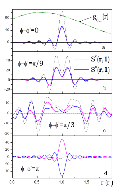
Figure 1: Dimensionless sums ${\cal S}^{o}({\bm{r}},{\bm{1}})$ and ${\cal S}^{e}({\bm{r}},{\bm{1}})$ given in Eq. (63) calculated numerically for nonsymmetric $2D$ Hooke’s atom in Eq. (58) for several values of relative phases $(\phi-\phi^{\prime})$. The dashed lines represent sums ${\cal S}^{o}({\bm{r}},{\bm{1}})+{\cal S}^{e}({\bm{r}},{\bm{1}})$ approximating delta function $\delta({\bm{r}}-{\bm{1}})$. In panel a) the dotted line indicates ground-state function $g_{0,1}(r)$ of $2D$ Hooke’s atom in Eq. (48).

The eigenenergies and eigenstates of the Hamiltonian in Eq. (58) are obtained by solving the problem of finite-size matrix: $\sum_{i^{\prime}}H_{ii^{\prime}}a_{i^{\prime}}=Ea_{i}$, where $a_{i}$ are uniquely obtained from $b_{m,n}$ by the mapping: $i\rightarrow(m,n)$. Using the inverse mapping $(m,n)\rightarrow i$ one has

$$H_{ii^{\prime}}=E_{i}\delta_{i,i^{\prime}}+qc_{m,m^{\prime}}\int_{0}^{\infty}\left[r^{2}g_{m,n}(r)g_{m^{\prime},n^{\prime}}(r)\right]rdr,$$ (60)

where for fixed $m$ the functions $g_{m,n}$ are normalized: $\int_{0}^{\infty}g_{m,n}(r)g_{m,n^{\prime}}(r)rdr=\delta_{n,n^{\prime}}$. The selection rules for $\phi$ integrals are

$$c_{m,m^{\prime}} = \frac{1}{2\pi}\int_{0}^{2\pi}e^{i(m-m^{\prime})\phi}\cos(\phi)^{2}d\phi$$ (61)

$$= \frac{1}{2}\delta_{m,m^{\prime}}+\frac{1}{4}\delta_{m,m^{\prime}\pm 2}.$$

The nonzero elements of $H_{ii^{\prime}}$ are those with $m^{\prime}=m$ and $m^{\prime}=m\pm 2$. Let $\{f_{l}^{e}(r,\phi)\}$ be a set of states of $H_{ii^{\prime}}$ obtained from even functions $g_{2m,n}(r)e^{(2m)i\phi}/\sqrt{2\pi}$, and $\{f_{l}^{o}(r,\phi)\}$ be a set of states of $H_{ii^{\prime}}$ obtained from odd functions $g_{2m+1,n}(r)e^{(2m+1)i\phi}/\sqrt{2\pi}$. Then

$$\hat{P}^{\eta}({\bm{r}},{\bm{r}}^{\prime})=\hat{H}({\bm{r}},{\bm{r}})\ {\cal S}^{\eta}({\bm{r}},{\bm{r}}^{\prime}).$$ (62)

where

$${\cal S}^{\eta}({\bm{r}},{\bm{r}}^{\prime})=\sum_{l}f_{l}^{\eta}(r,\phi)^{*}f_{l}^{\eta}(r^{\prime},\phi^{\prime}),$$ (63)

and $\eta\in\{e,o\}$. Note that for $l\rightarrow\infty$ there is: ${\cal S}^{e}({\bm{r}},{\bm{r}}^{\prime})+{\cal S}^{o}({\bm{r}},{\bm{r}}^{\prime})\rightarrow\delta({\bm{r}},{\bm{r}}^{\prime})$. In our calculations we take $4146$ $f_{l}^{e}(r,\phi)$ functions and $3908$ $f_{l}^{o}(r,\phi)$ functions, respectively.

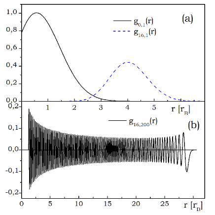
Figure 2: Functions $g_{m,n}(r)$ of 2D Hooke’s atom given in Eq. (49) calculated numerically for three $m,n$ values. Function $g_{0,1}(r)$ corresponds to the ground state of the system.

In Figure 1 we plot the sums ${\cal S}^{\eta}({\bm{r}},{\bm{r}}^{\prime})$ in Eq. (63) for ${\bm{r}}^{\prime}={\bm{1}}$ and several $(\phi-\phi^{\prime})$ values, where ${\bm{1}}$ is a unit vector in arbitrary direction. In our calculations we take $k_{y}=4$ and $k_{x}=9.61$, which gives $q=1.4025$, see Eq. (48). In Figure 1a there is $(\phi-\phi^{\prime})=0$ and both sums ${\cal S}^{\eta}({\bm{r}},{\bm{1}})$ tend to $\delta(r-1)$, where $r=|{\bm{r}}|$. We also plot the un-normalized function $g_{0,1}(r)$. It is seen that ${\cal S}^{\eta}$ are more localized than $g_{0,1}(r)$ which justifies treating ${\cal S}^{\eta}({\bm{r}},{\bm{1}})$ as approximations of $\delta(r-1)$ function.

By increasing $(\phi-\phi^{\prime})$ in Figures 1b and 1c the sums ${\cal S}^{\eta}({\bm{r}},{\bm{1}})$ gradually decrease, but they do not vanish because they are truncated to finite number of terms. For $(\phi-\phi^{\prime})=\pi$ in Figure 1d, the sum ${\cal S}^{e}({\bm{r}},{\bm{1}})$ tends to $\delta(r-1)$, while the sum ${\cal S}^{o}({\bm{r}},{\bm{1}})$ tends to $-\delta(r-1)$, so their sum practically cancels out (dotted line). The above results obtained numerically in Figure 1 for a non-separable function $f(r,\phi)$ illustrate general formulas in Eqs. (26)–(28).

We emphasize two approximations related to Figure 1. First, the summations over angular states are limited to $0\leq m\leq 16$, and the results may be incomplete because we omitted basis functions with higher $m$. Second, for fixed $m$ we take $n\simeq 250$ radial functions $g_{m,b}(r)$ and claim that they are sufficient to approximate combinations of delta functions in Eqs. (26) and (27). Both issues are clarified in Figures 2 and 3.

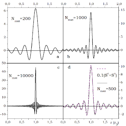
Figure 3: a), b), c) Dimensionless sums $S(x,x^{\prime})$ given in Eq. (64) for $1D$ harmonic oscillator functions calculated numerically for four $N_{max}$ values and $x^{\prime}=1$. d) Sum $S(x,1)$ calculated for $N_{max}=500$ compared with re-scaled sum ${\cal S}^{e}({\bm{r}},{\bm{1}})+{\cal S}^{o}({\bm{r}},{\bm{1}})$ defined in Eq. (63) and shown in Figure 1a, dashed line. The scaling factor is $c=0.1$.

In Figure 2 we show normalized functions $g_{0,1}(r)$ (ground state), $g_{16,1}(r)$, and $g_{16,200}(r)$. As seen from Figures 2b and 2c, functions having $m=16$ practically vanish at $r=1$ and they give negligible contributions to ${\cal S}^{\eta}({\bm{r}},{\bm{1}})$ for $0\leq r\leq 2$, see Eq. (63). This result confirms the validity of truncating the summation over $m$ states to $m\leq 16$ in Figure 1. Selecting larger $r^{\prime}$ and $r$ one has to include states with larger $m$.

To show that finite sums ${\cal S}^{\eta}$ in Figure 1 approximate the combinations of delta functions we consider the set of functions $\{\psi_{n}(x)\}$ being states of the one-dimensional harmonic oscillator with the potential $U(x)=x^{2}$. Let

$$S(x,x^{\prime})=\sum_{n}^{N_{max}}\psi_{n}(x)\psi_{n}(x^{\prime})\rightarrow\delta(x-x^{\prime}).$$ (64)

We calculate $S(x,x^{\prime})$ numerically using the recursion relation HermiteWiki : $\sqrt{\frac{n+1}{2}}\psi_{n+1}(x)=x\psi_{n}(x)-\sqrt{\frac{n}{2}}\psi_{n-1}(x)$ with the initial conditions: $\psi_{0}(x)=\pi^{-1/4}\exp(-x^{2}/2)$ and $\psi_{-1}(x)=0$. In Figure 3 we show $S(x,1)$ for several values of $N_{max}$. As seen in Figures 3a, 3b, and 3c, when increasing $N_{max}$ the sums $S(x,1)$ tend to $\delta(x-1)$. In Figure 3d we compare the sum $S(x,1)$ for $N_{max}=500$ with the re-scaled sum ${\cal S}^{e}({\bm{r}},{\bm{1}})+{\cal S}^{o}({\bm{r}},{\bm{1}})$ for $(\phi-\phi^{\prime})=0$ shown in Figure 1a. Both curves are close to each other up to a scaling factor $c=0.1$, which confirms the delta-like character of the curves shown in Figure 1.

As the third example we calculate the states and energies of the symmetric $2D$ Hooke’s atom described in Eq. (49) with use of Eqs. (41) and (42). We analyze odd states of $\hat{H}$, so we apply $\hat{P}^{o}$ operator, see Eq. (10). In the position representation $|{\bm{Q}}\rangle=|{\bm{R}},{\bm{r}}\rangle$ equations (41) and (42) read

$$\hat{H}\Psi({\bm{Q}})-\left(\hat{H}_{0}-\hat{P}^{o}_{0}\right)\Psi({\bm{Q}})=$$

$$\hat{H}\Psi({\bm{Q}})-\lambda\sum_{{\rm n}_{0}^{e}}E_{{\rm n}_{0}^{e}}\langle{\bm{Q}}|{\rm n}_{0}^{e}\rangle\int\langle{\rm n}_{0}^{e}|{\bm{Q}}^{\prime}\rangle\Psi({\bm{Q}}^{\prime})d^{2}{\bm{Q}}^{\prime}$$

$$=E\Psi({\bm{Q}}),\ \ \$$ (65)

and ${\bm{R}},{\bm{r}}$ are the center-of-mass and relative-motion coordinates, respectively. The superscript $e$ in Eq. (65) denotes even states and energies of $\hat{H}_{0}$, since the odd ones were eliminated by $\hat{P}^{o}_{0}$. Let

$$\Psi({\bm{R}},{\bm{r}}) = \frac{1}{\sqrt{2\pi}}F({\bm{R}})g_{m,n}(r)e^{im\phi},$$ (66)

$$\langle{\bm{R}},{\bm{r}}|{\rm n}_{0}^{a}\rangle = \frac{1}{\sqrt{2\pi}}F({\bm{R}})\psi_{2j,l}(r)e^{2ij\phi},$$ (67)

where $F({\bm{R}})$ satisfies Eq. (47), $g_{m,n}(r)$ is solution of Eq. (49), $\psi_{2j,l}(r)$ and $\epsilon_{2j,l}$ are functions and energies of $2D$ harmonic oscillator, respectively, $m,j$ describe angular momentum and $n,l$ label the discrete states. Functions $\psi({\bm{r}})=\psi_{2j,l}(r)e^{2ij\phi}$ in Eq. (67) are even: $\psi({\bm{r}})=\psi(-{\bm{r}})$. We approximate $\hat{\cal P}_{0}$ in Eq. (65) by restricting summations to few low-energy states: $j=0,\pm 1$ and $n=0,1,2$. For given $m$ and $n$ one has from Eq. (65)

$$\hat{H}_{r}g_{m,n}(r)\frac{e^{im\phi}}{\sqrt{2\pi}}-\lambda\sum_{l=0}^{2}\sum_{j=-1}^{1}\epsilon_{2j,l}\phi_{2j,l}(r)\frac{e^{2ij\phi}}{\sqrt{2\pi}}\times$$

$$\int_{0}^{\infty}\phi_{2j,l}(r^{\prime})g_{m,n}(r^{\prime})r^{\prime}dr^{\prime}\int_{0}^{2\pi}\frac{e^{i(m-2j)\phi^{\prime}}}{2\pi}d\phi^{\prime}$$

$$=E_{m,n}g_{m,n}(r)\frac{e^{im\phi}}{\sqrt{2\pi}},\ \ \ \ \$$ (68)

where $\hat{H}_{r}$ is defined in Eq. (49) and we used $\int|F({\bm{R}}^{\prime})d^{2}{\bm{R}}^{\prime}|^{2}=1$. The kernel corresponding to Eq. (68) is, see Eqs. (43) and (44)

$$\hat{K}({\bm{r}},{\bm{r}}^{\prime})=\sum_{l=0}^{2}\sum_{j=-1}^{1}\epsilon_{2j,l}\phi_{2j,l}(r)\phi_{2j,l}(r^{\prime})\frac{e^{2ij(\phi-\phi^{\prime})}}{2\pi}.$$ (69)

Now we discuss solutions of Eq. (68) for various values of $m$ and we analyze three cases: $m=\pm 1$, $m=0,\pm 2$ and $|m|>2$. Consider first two odd states with $m=\pm 1$. Since the second integral in Eq. (68) vanishes for $m=\pm 1$ one obtains

$$\hat{H}_{r}g_{m,n}(r)=E_{m,n}g_{m,n}(r),$$ (70)

i.e. Eq. (49). The solutions of Eq. (70) do not depend on $\lambda$. If in Eq. (68) one uses the kernel $\hat{K}_{1}({\bm{r}},{\bm{r}}^{\prime})$ of the form, see Eq. (44)

$$\hat{K}_{1}({\bm{r}},{\bm{r}}^{\prime})={\cal E}_{c}\sum_{j=-1}^{1}\phi_{2j,0}(r)\phi_{2j,0}(r^{\prime})\frac{e^{2ij(\phi-\phi^{\prime})}}{2\pi},$$ (71)

then for $g_{m,n}(r)$ one also obtains equation (70). In Eq. (71) the sum over $l$ is limited to a single term with $l=0$ and ${\cal E}_{c}$ is an arbitrary energy.

Consider now three even states with $m=0,\pm 2$. Then the sum over $j$ in Eq. (68) reduces to a single term with $2j=m$ and one has

$$\hat{H}_{r}g_{m,n}(r)-\lambda\sum_{l=0}^{2}\epsilon_{m,l}\phi_{m,l}(r)\int_{0}^{\infty}\phi_{m,l}(r^{\prime})g_{m,n}(r^{\prime})r^{\prime}dr^{\prime}$$

$$=E_{m,n}g_{m,n}(r).\ \ \ \ \ \ \$$ (72)

Equation (72) is differential-integral equation for unknown function $g_{m,n}(r)$, and it resembles Eq. (29). In Eq. (72) the function $g_{m,n}(r)$ does not vanish and it depends on $\lambda$. This also occurs when in Eq. (68) one replaces the kernel $\hat{K}({\bm{r}},{\bm{r}}^{\prime})$ by $\hat{K}_{1}({\bm{r}},{\bm{r}}^{\prime})$ in Eq. (71).

Consider now the exact operator $\hat{\cal P}$ instead of $\hat{\cal P}_{0}$. Then we set in Eq. (72) $\psi_{j,l}(r)\rightarrow g_{m,n}(r)$ and $\epsilon_{j,l}\rightarrow E_{m,n}$. For $m=0,\pm 2$ one has

$$\hat{H}_{r}g_{m,n}(r)-\lambda E_{m,n}g_{m,n}(r)=E_{m,n}g_{m,n}(r).$$ (73)

For $\lambda=1$ the left-hand-side of Eq. (73) vanishes, which gives $g_{m,n}(r)\equiv 0$, as expected from Eq. (38) for the exact $\hat{\cal P}$ operator.

Finally, for $|m|>2$ one obtains Eq. (70) both for odd and even $m$, since the approximate PEO in Eq. (68) contains only states with angular momenta $|m|\leq 2$. This also occurs for kernel $\hat{K}_{1}({\bm{r}},{\bm{r}}^{\prime})$ in Eq. (71).

From the above results we reach the following conclusions. First, by properly chosen set of $\langle{\bm{Q}}|{\rm n}_{0}^{a}\rangle$ states in Eqs. (41), (43) and (65) one can construct an approximate operator $\hat{\cal P}_{0}$ that does not alter odd (or even) states of the Hamiltonian and strongly affects the states of the opposite symmetry. Second, the use of simpler kernel in Eqs. (44) and (71) leads to qualitatively similar results to those obtained for the kernel in Eqs. (42) and (69). Third, the parameter $\lambda$ can be used as a tool for distinguishing states having proper or improper symmetry with respect to exchange of all pair of electrons. Finally, if one uses an approximate kernel in Eqs. (44) or (71), then they work correctly for some states only, in above example only for those with $|m|\leq 2$.

V Discussion

In this work we introduced the Pauli Exclusion Operator that ensures appropriate symmetry of multi-electron eigenstate, see Eqs. (7) and (8). For two-electron systems we showed three alternative representations of PEO. In Eqs. (9) and (10) we expressed PEO in terms of infinite sums over subsets of states belonging to the spectrum of the Hamiltonian. Using this method we calculated PEO for isotropic and anisotropic Hooke’s atom.

For $2D$ two-electron systems it is possible to express $\hat{P}$ in a closed form in terms of momentum operators, see Eqs. (21)–(23). In the position representation $\hat{P}$ is a nonlocal operator, and the states of the two-electron Hamiltonian should be calculated from the nonlocal Yamaguchi equation rather than the Schrodinger equation, see Eqs. (28) and (29).

In two-electron systems the spectrum of the Hamiltonian contains only symmetric or antisymmetric states. This is not valid in multi-electron cases, since for the latter the solutions of the Schrodinger equation may be symmetric for the exchange of some pairs of electrons and antisymmetric for the others. Only application of the Pauli exclusion principle selects states of $\hat{H}$ that are antisymmetric for exchange of all pairs of electrons.

The PEO can be generalized for multi-electron systems and it can be defined in two alternative forms: either in terms of operators $\hat{\chi}_{ij}$ [(see Eq. (33)] or by spectral resolution, see Eq. (36). The $\hat{\chi}_{ij}$ operators can be represented as a product of an infinite power series of position and momentum operators and electron spins. In this representation PEO depends on the product of $\hat{\chi}_{ij}$ for all pairs of electrons. In the second representation $\hat{\cal P}$ is an operator that includes all states and energies of the Hamiltonian except states being antisymmetric with respect to exchange of all pairs of electrons. For two-electron systems both forms of PEO reduce to results in Section II. Note that PEO can not be represented in a closed form for more than two electrons.

Several approximate formulas for $\hat{\cal P}$ were proposed in Section III. The most promising ones for multi-electron systems are based on the approximate forms of $\hat{\cal P}_{0}$ calculated for simpler systems as, e.g., for set of free electrons in harmonic potential, see Eq. (41). Another possibility is to treat $\hat{\cal P}_{0}$ as a kernel operator that ensures antisymmetry of the calculated wave function, see Eq. (42). This kernel may be treated as a mathematical object without clear physical meaning. Calculated energies and states of $2D$ Hooke’s atom confirm the effectiveness of these approximations.

It is interesting to compare results obtained with the use of PEO to variational methods for trial functions taken in form of Slater determinants. As shown in Eq. (45), once the wave function $|\Psi^{a}\rangle$ is already anti-symmetrized there is $\hat{\cal P}|\Psi^{a}\rangle=0$, and it is not necessary to introduce PEO. Variational calculations with the use of trial function in the Slater form are the most common method of calculating the energies and states of multi-electron systems. In practice this method is the best compared to other approaches. The conclusion is, that for variational calculations with the Slater determinants PEO is not needed.

However, if one goes beyond variational calculations or if a trial variational function is not antisymmetric in all pairs of electrons, then one encounters problem of ensuring antisymmetry of multi-electron function. This problem could be solved either ex-post, by eliminating spurious solutions that are not antisymmetric with respect to exchange of all pairs or electrons, or by adding PEO to the Hamiltonian that ensures antisymmetry of resulting wave function. As pointed above, it seems to be impossible to find exact PEO for arbitrary systems, but application of approximate forms of POE proposed in Section III may be sufficient to obtain a wave function fulfilling antisymmetry requirement.

The fundamental difference between PEO method and commonly used methods, as e.g. the configuration interaction (CI) method is as follows. In PEO approach one does not take any assumption of the wave function but the PEO ensures proper antisymmetry of the resulting wave function. In the CI method one does not introduce any additional operator, but assumes the multi-electron wave function as a combination of Slater determinants. Therefore the PEO method is in some sense ’opposite’ to commonly used methods based on Slater determinants. If both approaches, if one takes exact PEO or exact antisymmetric trial function the one obtains identical results. However, since in practice one always uses approximate methods, as e.g. those in Section III, it may turn out that in some problems one method is superior to the other. As an example, for $2D$ Hooke’s atom the use PEO gives exact energies and states, see Eq. (70), but variational method based on Slater determinants leads to approximate results.

In this work we concentrate on the analysis of the Pauli Exchange Operator for $2D$ Hooke’s atom, which is simpler than Hooke’s atom in $3D$. In the latter case the Hamiltonian also separates into parts depending on the center-of-mass motion and the relative motion. The states of the Hooke’s atom Hamiltonian in $3D$ have the form $\Psi({\bm{r}})=g_{l,n}(r)Y_{l,m}(\Theta,\phi)$, where $Y_{l,m}(\Theta,\phi)$ are the spherical harmonics in the standard notation. Functions $g_{l,m}(r)$ are the solutions of the equation

$$\left(-\frac{d^{2}}{dr^{2}}-\frac{2}{r}\frac{d}{dr}+\frac{l(l+1)}{r^{2}}+\frac{1}{r}+\frac{k}{4}r^{2}\right)g_{l,n}(r)=E_{l,n}g_{l,n}(r),$$ (74)

where $l=0,1\ldots$ is angular momentum number and $E_{l,n}$ are the energies. Functions $g_{l,n}(r)$ in Eq. (74) are similar to $g_{m,n}(r)$ in Eq. (49), see Figure 2. In $3D$ the transformation ${\bm{r}}\rightarrow-{\bm{r}}$ does not change $r=|{\bm{r}}|$ coordinate, but changes the angular functions

$$Y_{l,m}(\Theta,\phi)\rightarrow Y_{l,m}(\pi-\Theta,\phi+\pi)=(-1)^{l}Y_{l,m}(\Theta,\phi).$$ (75)

Then, similarly to $2D$ case, the states with even $l$ are symmetric with respect to exchange of electrons, while those with odd $l$ are asymmetric. In $3D$ one may not express $\hat{P}$ in terms of differential operator, because the transformation $\Theta\rightarrow\pi-\Theta$ can not be expressed in terms of translation operator, see Eqs. (14) and (23). However, representation of PEO in Eqs. (26)–(28) is valid also in $3D$ Hooke’s atom model.

There exist two systems having two interacting electrons, i.e. the helium atom and the lithium ion. In these systems the external potential acting on the electrons is the Coulomb potential of the nucleus. The Schrodinger equations of both systems do not separate into the center-of-mass and relative motions, and in order to find eigenvalues or the eigenstates one has to use approximate methods, e.g. variational calculations, molecular orbital approximations or perturbation methods BetheBook ; Tanner2000 . These methods work correctly for low energy states but their accuracy decreases for high-energies. For this reason it is practically impossible to calculate PEO for helium atom and lithium ion by summating the eigenstates in Eqs. (9) and (10). However, the results in Figures 1 and 3 suggest that for both systems the position representation of PEO is also given in Eqs. (26)–(28). Finally, for hypothetical $2D$ helium atom PEO is also given by Eq. (23).

Let us briefly discuss some issues related to spin part of wave function for multi-electron systems. Consider first the three-electron case as e.g. the lithium atom and assume that the Hamiltonian of the system does not depend on electron spins. In such a case the wave function of the system is a product of position-dependent and spin-dependent functions. For three spins there is $2^{3}$ spins-combinations, and they form four quartets and four doublets Buchachenko2002 . The quartet states are symmetric with respect to exchange of three pairs of spins, but doublets are not, so to ensure proper symmetry of three-electron wave function a combination of doublets should be taken. For $k$-electron system there is $2^{k}$ spins combinations, and for large $k$ it is practically impossible to treat spins exactly, so one may either treat them classically, or apply further approximations.

In Section II we assumed spin-independent two-body Hamiltonian. In real systems one often meets spin-dependent interactions, usually related to the spin-orbit (SO) coupling. In practical realizations of Hooke’s-like systems in quantum dots the SO is common, see Darnhofer1993 ; Jacak1997 ; Poszwa2020 . In the standard notation there is $\hat{H}_{SO}=\alpha\hat{\bm{L}}\cdot\hat{\bm{S}}$, and for $L>0$. Then, for $L>0$ the wave functions of electrons do not separate in position-only and spin-only parts and we may not use the approach in Section II. The general formalism in Section III as well as the approximate methods are valid also for systems with spin-dependent interactions including SO.

For two-electron systems in Section II the PEO is defined as an operator that removes even or odd states from the Hamiltonian spectrum. Then the function $|\Psi\rangle$, being the solution of $\left(\hat{H}-\hat{P}\right)|\Psi\rangle=E|\Psi\rangle$, includes odd or even states only. For multi-electron systems in Section III the PEO is defined as an operator that removes antisymmetric states with respect to exchange of all pairs of electrons from Hamiltonian spectrum. Then the function $|\Psi\rangle$, being the solution of $\left(\hat{H}-\hat{\cal P}\right)|\Psi\rangle=E|\Psi\rangle$, includes antisymmetric states only. The difference between both definitions is that even or odd states of two-electron system relate to relative motion of electrons, while for multi-electron systems the antisymmetry relates to exchange of two electrons including their positions and spins.

PEO in literature appear previously in calculations of nuclear matter properties Cheon1989 ; Schiller1999 ; Suzuki2000 . In the approach of Ref. Suzuki2000 the $\hat{G}$ matrix satisfies the Bethe-Goldstone equation

$$\hat{G}=v+v\frac{\hat{Q}}{\epsilon}\hat{G},$$ (76)

where $\hat{G}$ is the reaction matrix, $v$ is the two-nucleon interaction, $\epsilon$ is re-scaled energy and $\hat{Q}$ is PEO in nuclear matter which prevents two particles from scattering into intermediate states with momenta below the Fermi energy. In some aspects this approach is similar to ours since the authors introduce an operator responsible for the Pauli exclusion principle, but PEO in the previous approach excludes some states from real or virtual scattering. In our approach PEO ensures proper symmetry of multi-electron wave function.

VI Summary

In this work we introduce the Pauli Exclusion Operator which ensures proper symmetry of the states of multi-electron systems with respect to exchange of each pair of electrons. Once PEO is added to the Hamiltonian, no additional constraints due to the Pauli exclusion principle need to be imposed to multi-electron wave function. PEO is analyzed for two-electron Hamiltonian and we found its three representations. We concentrated on PEO in $2D$ in which it can be expressed in closed form. Some properties of PEO in $3D$ and $1D$ for two-electron states are discussed. PEO are calculated analytically or numerically for symmetric and antisymmetric Hooke’s atoms. We generalized PEO for multi-electron systems; its two alternative forms are obtained. Several approximations of PEO to multi-electron systems were derived. Kernel-based methods were proposed, and they seem to be most promising approximations of PEO for practical calculations. It is shown that once the wave function $|\Psi^{a}\rangle$ is already antisymmetric with respect to exchange of all pairs of electrons, $\hat{\cal P}|\Psi^{a}\rangle$ identically vanishes. For this reason, in variational calculations employing trial functions in the form of Slater determinants there is no need to introduce PEO. However, if one goes beyond variational calculations, one should introduce PEO to ensure antisymmetry of the resulting wave functions. We believe that the approach based on exact, approximate or kernel forms of PEO may be useful in calculating energies and states of multi-electron systems.

Appendix A Auxiliary identities

The spin-exchange operator $\hat{\Sigma}_{ij}$ is defined by its action on four two-spin states

$$\hat{\Sigma}_{ij}|\uparrow\uparrow\rangle=|\uparrow\uparrow\rangle,$$ (77)

$$\hat{\Sigma}_{ij}|\uparrow\downarrow\rangle=|\downarrow\uparrow\rangle,$$ (78)

$$\hat{\Sigma}_{ij}|\downarrow\uparrow\rangle=|\uparrow\downarrow\rangle,$$ (79)

$$\hat{\Sigma}_{ij}|\downarrow\downarrow\rangle=|\downarrow\downarrow\rangle.$$ (80)

Operator $\hat{\Sigma}_{ij}$ in Eq. (32) satisfies all above equations.

In $3D$ the particle exchange operator is given in Eq. (23) of Ref. Schmid1979 and for completeness we quote this expression

$$\hat{\Pi}_{ij}=\sum_{n=0}^{\infty} \left(\frac{1}{n!}\right)\left(\frac{i}{\hbar}\right)^{n}\sum_{l=0}^{n}\sum_{m=0}^{l}\left(\begin{array}[]{c}n\\ l\end{array}\right)\left(\begin{array}[]{c}l\\ m\end{array}\right)$$

$$\times \left(\hat{p}_{jx}-\hat{p}_{ix}\right)^{n-l}\left(\hat{r}_{jx}-\hat{r}_{ix}\right)^{n-l}$$

$$\times \left(\hat{p}_{jy}-\hat{p}_{iy}\right)^{l-m}\left(\hat{r}_{jy}-\hat{r}_{iy}\right)^{l-m}$$

$$\times \left(\hat{p}_{jz}-\hat{p}_{iz}\right)^{m}\left(\hat{r}_{jz}-\hat{r}_{iz}\right)^{m}.$$ (86)

By taking limit $\Delta\hat{x}_{ij}\rightarrow 0$ in Eq. (A) one obtains the particle exchange operator in $2D$

$$\hat{\Pi}_{ij}=\sum_{n=0}^{\infty} \left(\frac{1}{n!}\right)\left(\frac{i}{\hbar}\right)^{n}\sum_{l=0}^{n}\left(\begin{array}[]{c}n\\ l\end{array}\right)$$

$$\times \left(\hat{p}_{jx}-\hat{p}_{ix}\right)^{n-l}\left(\hat{r}_{jx}-\hat{r}_{ix}\right)^{n-l}$$

$$\times \left(\hat{p}_{jy}-\hat{p}_{iy}\right)^{l}\left(\hat{r}_{jy}-\hat{r}_{iy}\right)^{l}.$$ (90)

Alternative expressions for $\hat{\Pi}_{ij}$ is given in Grau1981 .

Appendix B Shooting method

The eigenenergies and eigenstates of Hooke’s atom in Eq. (49) are found using shooting method NRecBook . As the initial guesses for the energies we use those of two-dimensional harmonic oscillator equal to $E_{n}=\sqrt{(k/4)}(2n+1)$, $n=0,1,..\ldots$m and $k=4$. Then we iteratively bracket the true energies of $\hat{H}$ by analyzing behavior of $g_{m,n}(r)$ at large $r$. The advantage of the shooting method is that it is equally accurate for low and high energy states. Only functions with $m\geq 0$ were calculated since $g_{-m,n}(r)=g_{m,n}(r)$. We tabulate normalized states of Eq. (49) from $n=1$ (ground state) to $n=250$ and from $m=0$ to $m=16$.

We solve Eq. (49) using DVERK procedure which is $6-$th order Runge-Kutta method Verner1971 ; HairerBook . The accuracy of calculations has been verified by checking the orthogonality of all pairs of $g_{m,n}(r)$ and $g_{m^{\prime},n^{\prime}}(r)$ functions with $m=m^{\prime}$ and $n\neq n^{\prime}$. In each case the accuracy below $10^{-5}$ has been obtained.

For small $r$ there is: $g_{0,n}(r)\simeq c_{0}(1+r)$ with $c_{0}>0$, and the initial conditions for DVERK procedure are: $g_{0,n}(0)=1$, $g_{0,n}^{\prime}(0)=h$, where $h$ is the integration step, and $h\simeq 0.001-0.01$ r_B. For $m>0$ and small $r$ there is: $g_{m,n}(r)\propto r^{m}$, and the initial conditions for DVERK procedure are: $g_{m,n}(0)=0$, $g_{m,n}^{\prime}(0)=mh^{m-1}$. For large $m$ the last condition is unstable numerically, and it is replaced by: $g_{m,n}(r_{0})=g_{c}$, $g_{m,n}^{\prime}(r_{0})=mg_{c}/r_{0}$, $g_{c}\simeq 10^{-5}$, and $g_{m,n}(r)=0$ for $r<r_{0}$. Here $r_{0}>0$ and its values for $g_{m,n}(r)$ are obtained by analysis of $g_{m-1,n}(r)$ for small $r$. Generally, $r_{0}$ gradually increases with $m$.

References

- (1) G. W. Kellner, Z. Phys. 44, 91 (1927).
- (2) E. A. Hylleraas, Z. Phys. 48, 469 (1928).
- (3) E. A. Hylleraas, Z. Phys. 54, 347 (1929).
- (4) W. Pauli, Zeits. Phys. 31, 765 (1925).
- (5) W. Pauli, Phys. Rev. 58, 715 (1940).
- (6) H. A. Bethe and E. E. Salpeter Quantum Mechanics of One- and Two-electron Atoms (Academic Press, New York, 1957).
- (7) G. Tanner, K. Richter and J. M. Rost, Rev. Mod. Phys. 72, 497 (2000).
- (8) T. Cheon and E. F. Redish, Phys. Rev. C 39, 331 (1989).
- (9) E. Schiller, H. Muther, and P. Czerski, Phys. Rev. C 59, 2934 (1999); Phys. Rev. C 60, 059901(E) (1999).
- (10) K. Suzuki, R. Okamoto, M. Kohno, and S. Nagata, Nucl. Phys. A665, 92 (2000).
- (11) S. Kais, D. R. Herschbach, and R. D. Levine, J. Chem. Phys. 91, 7791 (1989).
- (12) M. Taut, Phys. Rev. A 48, 3561 (1993).
- (13) M. Taut, J. Phys. A 27, 1045 (1994).
- (14) D. P. O’Neill and P. M. W. Gill, Phys. Rev. A 68, 022505 (2003).
- (15) https://en.wikipedia.org/wiki/Hooke%27s_atom, (2020).
- (16) https://en.wikipedia.org/wiki/Translation_operator _(quantum_mechanics), (2020).
- (17) Y. Yamaguchi, Phys. Rev. 95, 1628 (1954).
- (18) B. Schmid, Am. J. Phys. 47, 166 (1979).
- (19) D. Grau, Am. J. Phys. 49, 669 (1981).
- (20) https://en.wikipedia.org/wiki/Hermite_polynomials, (2020).
- (21) A. L. Buchachenko and V. L. Berdinsky, Chem. Rev. 102, 603 (2002).
- (22) T. Darnhofer and U. Rossler, Phys. Rev. B 47, 16020 (1993)
- (23) L. Jacak, J. Krasnyj, and A. Wojs, Physica B 229, 279 (1997).
- (24) A. Poszwa Act. Phys. Pol. A 138, 477 (2020).
- (25) W. H. Press, S. A. Teukolsky, W. T. Vetterling, and B. P. Flannery Numerical Recipes: The Art of Scientific Computing (3rd ed.), (New York: Cambridge 2007), Section 18.1.
- (26) J. H. Verner, Proc. Conf. Appl. Numer. Analysis, Lecture Notes in Mathematics 228, Springer Verlag, p. 340 (1971).
- (27) E. Hairer, S. P. Norsett, and G. Wanner, Solving Ordinary Differential Equations I, Nonstiff Problems (2nd ed.), (Springer Series in Computational Mathematics, Berlin, 1993) p. 181, Table 5.4.