Initial operation and data processing on a system for real-time evaluation of Thomson scattering signals on the Large Helical Device

Abstract

A scalable system for real-time analysis of electron temperature and density based on signals from the Thomson scattering diagnostic, initially developed for and installed on the NSTX-U experiment, was recently adapted for the Large Helical Device (LHD) and operated for the first time during plasma discharges. During its initial operation run, it routinely recorded and processed signals for four spatial points at the laser repetition rate of 30 Hz, well within the system’s rated capability for 60 Hz. We present examples of data collected from this initial run and describe subsequent adaptations to the analysis code to improve the fidelity of the temperature calculations.

I Introduction

The ability to determine plasma temperature and density profiles in real time is valuable to plasma control systems seeking to optimize plasma properties or maintain device safety. The Thomson scattering diagnostic is an attractive candidate for real-time profile evaluation due to its ability to make non-invasive measurements of electron temperature $T_{e}$ and electron density $n_{e}$ throughout a typical fusion plasma.Hutchinson (2002) In addition, the localized nature of the measurement obviates the need for intermediate analysis such as tomographic inversion or equilibrium modeling to infer the profiles.

Systems for evaluating Thomson scattering data in real time have been developed for a number of devices over the years.Greenfield et al. (1990); Shibaev et al. (2010a, b); Kolemen et al. (2015); Arnichand et al. (2019) In this work, we use a framework that was developed recently for NSTX-ULaggner et al. (2019) but has not yet been tested during plasma discharges. Its main components are a set of fast digitizers and a multi-core server. The digitizers collect signals from the detection electronics. The server employs real-time software to calculate $T_{e}$ and $n_{e}$ from the signals between subsequent laser pulses, supporting repetition rates of up to 60 Hz.Rozenblat et al. (2019) The server outputs $T_{e}$, $n_{e}$, and their uncertainties for each scattering volume as analog signals that may be fed into control systems.

The setup was subsequently replicated and installed on the Large Helical Device (LHD) to evaluate signals from the LHD Thomson scattering system. This system currently employs four Nd:YAG lasers that enable pulse repetition rates ranging from 10 to 100 Hz.Yamada et al. (2016) Backscattered light is transmitted through optical fibers to a set of 144 polychromators.Narihara et al. (1997, 2001) Within each polychromator, the scattered light passes through bandpass filters to six avalanche photodiodes (APDs).Yamada et al. (2010) Signals from five of these APDs are used for $T_{e}$ and $n_{e}$ evaluation during plasma discharges, and the remaining signal is used for Rayleigh calibration.Yamada et al. (2007) As the setup is similar to what is employed in NSTX-U,LeBlanc et al. (2003); Diallo et al. (2012) the real-time framework could be adapted for LHD with minor modifications.

During its initial operation on LHD, the real-time system collected and evaluated signals from four polychromators. For these experiments, laser pulses occurred at a 30 Hz repetition rate. In addition to performing $T_{e}$ and $n_{e}$ calculations for each pulse, the real-time system archived the polychromator signals at the end of each discharge, thereby enabling a postmortem assessment of the real-time calculations. In this paper, we describe this assessment, with a focus on the methods used for processing the raw polychromator signals. In Sec. II, we assess three signal-processing methods. Then, in Sec. III, we compare the values of $T_{e}$ and $n_{e}$ derived from each of these methods with the values calculated by the standard LHD methods performed after each discharge.

II Signal processing methods

The real-time system computes $T_{e}$ and $n_{e}$ values in a least-squares spectral fitting technique that optimizes $T_{e}$ and a scaling factor $c$ to minimize $\chi^{2}$, defined as follows:

$$\chi^{2}=\sum_{i=1}^{N_{c}}\frac{\left(s_{i}-cF_{i}(T_{e})\right)^{2}}{\sigma_{s_{i}}^{2}+s_{i}^{2}\sigma_{F_{i}}^{2}}$$ (1)

Here, $N_{c}$ is the number of polychromator channels (five for LHD) and $F_{i}(T_{e})$ is the expected relative signal strength from the $i$th channel for electron temperature $T_{e}$. The electron density $n_{e}$ can then be determined from $c$ along with calibration data. $s_{i}$ is a measure of the signal strength from the $i$th polychromator channel. $\sigma_{s_{i}}$ is the standard error in the $s_{i}$ measurement, and $\sigma_{F_{i}}$ is the (dimensionless) fractional error in $F_{i}$.

As described in Ref. Laggner et al., 2019, the values of $F_{i}$ are pre-computed for a range of $T_{e}$ by integrating the measured transmissivity spectrum of the $i$th polychromator channel with the Thomson scattering spectrum as predicted by the Selden model.Selden (1980) Fig. 1 shows transmissivity curves for one polychromator, along with scattering spectra for selected values of $T_{e}$. Evaluation of $F_{i}(T_{e})$ between laser pulses entails querying a table of the pre-computed values.

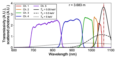
Figure 1: Transmissivity spectra of the five channels of the polychromator surveying the scattering volume at $r=3.683$ m, along with Thomson scattering spectra for three example electron temperatures.

$s_{i}$ in Eq. 1 must be proportional to the number of scattered photons received by the i^th channel. In this section, we will describe three procedures for deriving $s_{i}$ from polychromator signals and compare their accuracy and computational requirements. The procedures, which include peak detection, direct integration, and curve fitting, are displayed schematically in Fig. 2 with examples of two types of raw signals. The first type (Fig. 2a-c) is a response to the firing of a single laser and will be categorized as a “single laser pulse,” whereas the second type (Fig. 2d-f) arises from two lasers firing in rapid succession along the same beam path and will be categorized as a “double laser pulse.”

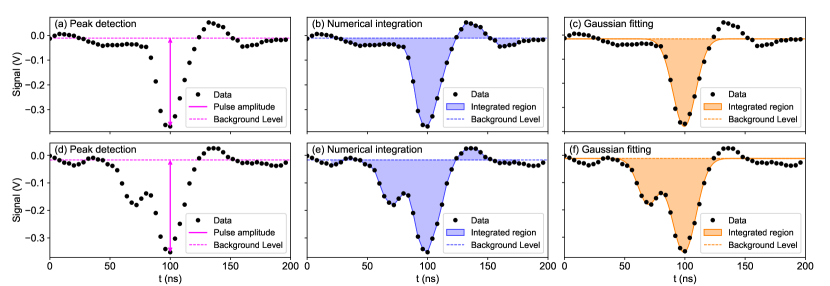
Figure 2: Typical signal from a polychromator channel along with depictions of the three methods for evaluation considered in this work: (a) peak detection, (b) numerical integration, and (c) Gaussian curve-fitting for a signal arising from light scattered from a single laser pulse; (d)-(f) like (a)-(c) but for a signal arising from light scattered from two overlapping laser pulses.

Each procedure was implemented as a C++11 function that could be called by the real-time software. The functions each took a digitized raw signal as input and returned values for $s_{i}$ and $\sigma_{s_{i}}$. The computational expense of each procedure was determined by recording the time required for its respective function to process archived experimental signals. These tests were performed on the same type of processing hardware employed in the experimental setup, i.e. a SuperMicro real-time server with 32 GB RAM and 20 cores clocked at 2.1 GHz.Laggner et al. (2019); Rozenblat et al. (2019)

We will use function evaluation times to determine how much each procedure will add to the system’s end-to-end processing time. This duration, which includes digitization, signal evaluation, plasma parameter calculation, and output signal generation, was previously determined in offline tests to be less than 16.7 ms with the peak detection procedure. While the calculations for each scattering volume are performed in parallel threads, the values of $s_{i}$ and $\sigma_{s_{i}}$ for each polychromator channel are determined in series. Hence, we will estimate the additional end-to-end-time required for a given procedure as the time by which the evaluation of the five signals from a polychromator with the procedure exceeds that of peak detection. To accommodate the 30 Hz laser repetition rate used during the LHD experiments, the total time should not exceed 33.3 ms.

II.1 Peak detection

As originally designed, the software worked on the assumption that the photon flux to each polychromator channel would scale directly with the peak amplitude of its signal. Hence, it would suffice to define $s_{i}$ simply as the peak amplitude in order to determine $T_{e}$. Provided that the signals from absolute calibrations are evaluated in the same way, a consistent scaling factor may be determined for extracting $n_{e}$ from $c$.

The real-time code determines the amplitude of the scattered-light signal during each laser pulse by subtracting the peak value of the signal from the average of the background signal recorded prior to the laser pulse. The procedure is illustrated in Fig. 2a for the case of a single laser pulse and in Fig. 2d for a double pulse. The background level, illustrated by the horizontal dashed line, is obtained as the average of a group of sample points separated from the peak by at least 80 ns. To correct for stray laser light due to reflections within the plasma vessel, this amplitude would be adjusted by subtracting the average signal amplitude recorded during laser pulses prior to the beginning of the discharge from the corresponding scattering volume and polychromator channel.

This approach has the advantage of simplicity and speed. However, the amplification circuitry, which in this setup includes a high-pass filter, may exhibit a dispersive or nonlinear response that would give rise to distortions of the signal that can vary from one channel to another. Evidence of this response can be seen in the overshoot of the signal above the background level following the peak in the examples shown in Fig. 2.

The effect of such distortions in the fitting of the polychromator output spectra is visible in Fig. 3a, which compares fitted data $s_{i}/c$ with the predicted signals $F_{i}(T_{e})$ acquired from one scattering volume during an example plasma discharge. These fits contain substantial systematic errors. In particular, the fitted signal amplitudes are mostly lower than the model prediction for polychromator channels 3 and 5, whereas they are mostly higher than the model prediction for channel 4.

Figure 3: Comparison of calibration spectra with fitted polychromator signals from the scattering volume at $r=3.683$ m. Solid curves represent $F_{i}(T_{e})$ from each polychromator channel. Circles represent $s_{i}/c$, positioned to $T_{e}$ according their respective fits. Signals determined through (a) peak detection; (b) numerical integration; (c) integration of a Gaussian fit curve.

II.2 Numerical integration

In the presence of distorted polychromator signals, the integrals of the signals may provide a more accurate representation of the detected scattered light than the amplitudes alone. To test this, we implemented a modified version of the signal processing function that performs trapezoidal integration on an interval of the signal of pre-determined length centered around the peak value. This procedure is illustrated schematically in Fig. 2b and 2e. Analogously to the case of pulse amplitude determination, the integrals of signals recorded during the plasma discharge were corrected by subtracting the average integral value of a set of stray laser light signals obtained prior to the plasma discharge.

The switch to numerical integration has minimal impact on computation time, with each integration taking $\leq~{}1~{}\mu$s longer than a corresponding amplitude determination. Hence, to evaluate the five polychromator outputs necessary for a spectral fit, the added time would not exceed 5 $\mu$s. This is negligible compared to the laser firing period of $16.7$ ms for which the system was designed.

As shown in Fig. 3b, the use of integrated signals improved the quality of the spectral fits. In particular, the systematic offsets between the data and the fitted spectra that arose from the use of pulse amplitudes (Fig. 3a) are no longer visible.

While the use of numerical integration removed the systematic offsets, the fits did exhibit increased scatter, particularly for the weaker signals from channel 5. This may arise from background noise, which can make spurious contributions to the integral in the case of a low signal-to-noise ratio (SNR) as seen in Fig. 2b and 2e. As the background fluctuations in the raw signal exhibit time scales similar to the laser pulse width, their contributions to the integral will not necessarily cancel out.

II.3 Curve fitting

One way to avoid contributions from background fluctuations is to integrate a waveform fitted to the signal rather than the raw signal itself.Kurzan et al. (2004); Bozhenkov et al. (2017) To this end, we implemented an additional function that fits Gaussian curves to the signal and outputs the integrals computed analytically from the fitting parameters. Specifically, signals were fit to functions of the form

$$f(t)=p_{1}+p_{2}\exp\left[-\frac{(t-p_{4})^{2}}{2p_{3}^{2}}\right]+p_{5}\exp\left[-\frac{(t-p_{7})^{2}}{2p_{6}^{2}}\right]$$ (2)

with free parameters $p_{1...7}$. For single laser pulses, $p_{5}=0$, and $p_{6}$ and $p_{7}$ were ignored. The true signal waveform is not exactly Gaussian due to the effects of the amplifier circuitry. However, a more precise model would be more computationally expensive, and we expect that the Gaussian fits will be accurate enough for the purposes of real-time analysis.

The parameters $p_{i}$ are determined in a Levenberg-Marquardt least-squares fitting procedure. The integrals of the fitted curves follow as $\sqrt{2\pi}p_{2}p_{3}$ for single pulses and $\sqrt{2\pi}(p_{2}p_{3}+p_{5}p_{6})$ for double pulses. The choice of whether to fit to a single or double pulse can be made based on laser energy signals: if two lasers fire, a double pulse is fitted; otherwise, a single pulse is fitted.

The curve-fitting approach requires substantially more complex computations than the previous approaches. Each least-squares iteration requires at least two evaluations of the exponential function for each time point within the integration window, as well as the inversion of an an $n\times{n}$ matrix, where $n$ is the number of free parameters. We employed the Armadillo C++ linear algebra librarySanderson and Curtin (2016, 2018) to ensure efficient matrix inversion.

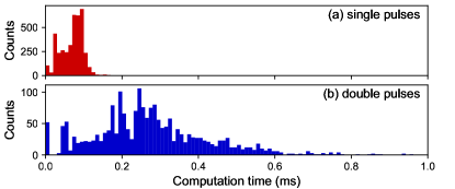
Figure 4: Histograms of the total computation time required to evaluate signal amplitudes from each of five polychromator channels using curve fitting. (a) Single laser pulses; (b) double laser pulses.

Evaluation times for curve-fitting during a survey of five example shots are shown in Fig. 4. Each sample corresponds to the total time to evaluate fitting parameters for signals from each of five polychromator channels from a single scattering volume for a particular laser pulse during a given discharge. Values near zero correspond to samples in which all the signals from a polychromator were less than their respective SNR (occurring, e.g., at the beginnings and ends of discharges), in which case the procedure would not attempt any fits. Overall, the computation time to process five polychromator signals was less than 110 $\mu$s in 95% of cases for single laser pulses. For double pulses, the total time was less than 550 $\mu$s in 95% of cases, although a number of outliers required more than 800 $\mu$s.

As stated previously, the real-time system with its original software has an end-to-end processing time of 16.7 ms or less. Hence, in a worst-case performance scenario in which the system requires a full 16.7 ms to complete its operations for a laser pulse, replacing the peak-detection procedure with curve-fitting could extend the required processing time by 0.5 ms to 1 ms. Under these conditions, the system could not accommodate laser pulses at the 60 Hz repetition rate for which it was originally designed. However, it could still accommodate rates of up to 50 Hz, which would have cycle deadlines of $\geq$20 ms. In particular, the incorporation of curve-fitting would still work on LHD when a 30 Hz rate is employed.

III Temperature and density calculations

Fig. 5 compares example $T_{e}$ and $n_{e}$ estimates using the three different procedures described in Sec. II. The reference values $T_{e,\text{ref}}$ and $n_{e,\text{ref}}$ were obtained from the standard LHD post-processing routines. The real-time functions calculated $n_{e}$ using the values of $c$ (Eq. 1) scaled and offset by calibration factors determined through fitting to $n_{e,\text{ref}}$ obtained from a separate set of discharges, independently for single and double laser pulses. Points with $n_{e}<0.5\times 10^{-19}$ m^-3 and $T_{e}>4$ keV generally had high uncertainty for this example and were omitted from the plot.

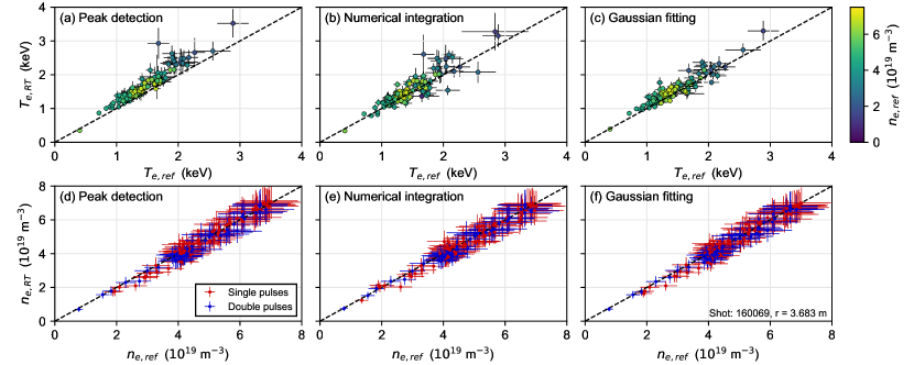
Figure 5: Comparison of $T_{e,\text{RT}}$ and $n_{e,\text{RT}}$ calculated by functions from the real-time code employing different signal-processing methods with reference values $T_{e,\text{ref}}$ and $n_{e,\text{ref}}$ calculated by the standard LHD post-processing routines. (a)-(c) $T_{e}$ with color scaling according to $n_{e}$; (d)-(f) $n_{e}$, colored according to pulse type.

Overall, the values of $T_{e}$ and $n_{e}$ as computed by all three methods track well with the reference values, almost always agreeing to within 0.5 keV and $0.5\times 10^{19}$ m^-3. In general, the real-time software tends to slightly overestimate $T_{e}$ relative to the reference values. Note that the overestimation of $T_{e}$ is most severe for the peak-detection method (Fig. 5a), an effect that we believe is related to the systematic errors in the spectral fitting for this method. The values of $T_{e}$ determined from numerical integration exhibit greater scatter than the other methods due to the impacts of noise on the integration: the standard deviation of $T_{e}-T_{e,\text{ref}}$ was $190$ eV for the numerical integration approach, whereas it was $160$ eV for the pulse amplitude approach and $130$ eV for curve fitting. The tendency of curve-fitting methods to produce $T_{e}$ values with less scatter than direct integration has also been observed, for example, in the Thomson scattering system at KSTAR.Lee et al. (2017)

IV Conclusions

In summary, we have adapted and commissioned a real-time evaluation system for Thomson scattering on the LHD experiment, representing the first in situ operation of the system. We have implemented and compared three different approaches to evaluating the polychromator signals, each of which offers advantages and disadvantages. The curve fitting approach generally provides the greatest accuracy and precision, but at the expense of extra computation time. Nevertheless, initial comparisons of $T_{e}$ and $n_{e}$ output by all three methods mostly exhibit good agreement with values calcuated by the standard post-processing software.

Data availability

The data supporting the findings of this study are available at http://arks.princeton.edu/ark:/88435/dsp014t64gr25v.

References

- Hutchinson (2002) I. Hutchinson, Principles of Plasma Diagnostics, 2nd ed. (Cambridge University Press, 2002).
- Greenfield et al. (1990) C. M. Greenfield, G. L. Campbel, T. N. Carlstrom, J. C. DeBoo, C.-L. Hsieh, R. T. Snider, and P. K. Trost, Review of Scientific Instruments 61, 3286 (1990).
- Shibaev et al. (2010a) S. Shibaev, G. Naylor, R. Scannell, G. McArdle, T. O’Gorman, and M. J. Walsh, Fusion Engineering and Design 85, 683 (2010a).
- Shibaev et al. (2010b) S. Shibaev, G. Naylor, R. Scannell, G. J. McArdle, and M. J. Walsh, in Proceedings of the 17th IEEE-NPSS Real Time Conference (2010).
- Kolemen et al. (2015) E. Kolemen, S. L. Allen, B. D. Bray, M. E. Fenstermacher, D. A. Humphreys, A. W. Hyatt, C. J. Lasnier, A. W. Leonard, M. A. Makowski, A. G. McLean, R. Maingi, R. Nazikian, T. W. Petrie, V. A. Soukhanovskii, and E. A. Unterberg, Journal of Nuclear Materials 463, 1186 (2015).
- Arnichand et al. (2019) H. Arnichand, Y. Andrebe, P. Blanchard, S. Antonioni, S. Couturier, J. Decker, B. P. Duval, F. Felici, C. Galperti, P.-F. Isoz, P. Lavanchy, X. Llobet, B. Marlétaz, P. Marmillod, J. Masur, and the TCV team, Journal of Instrumentation 14, C09013 (2019).
- Laggner et al. (2019) F. M. Laggner, A. Diallo, B. P. LeBlanc, R. Rozenblat, G. Tchilinguirian, E. Kolemen, and the NSTX-U team, Review of Scientific Instruments 90, 043501 (2019).
- Rozenblat et al. (2019) R. Rozenblat, E. Kolemen, F. M. Laggner, C. Freeman, G. Tchilinguirian, P. Sichta, and G. Zimmer, Fusion Science and Technology 75, 835 (2019).
- Yamada et al. (2016) I. Yamada, H. Funaba, R. Yasuhara, H. Hayashi, N. Kenmochi, T. Minami, M. Yoshikawa, K. Ohta, J. H. Lee, and S. H. Lee, Review of Scientific Instruments 87, 11E531 (2016).
- Narihara et al. (1997) K. Narihara, K. Yamauchi, I. Yamada, T. Minami, K. Adachi, A. Ejiri, Y. Hamada, K. Ida, H. Iguchi, K. Kawahata, T. Ozaki, and K. Toi, Fusion Engineering and Design 34-35, 67 (1997).
- Narihara et al. (2001) K. Narihara, I. Yamada, H. Hayashi, and K. Yamauchi, Review of Scientific Instruments 72, 1122 (2001).
- Yamada et al. (2010) I. Yamada, K. Narahara, H. Funaba, T. Minami, H. Hayashi, T. Kohmoto, and the LHD experiment group, Fusion Science and Technology 58, 345 (2010).
- Yamada et al. (2007) I. Yamada, K. Narihara, H. Hayashi, H. Funaba, and the LHD experiment group, Plasma and Fusion Research 2, S1106 (2007).
- LeBlanc et al. (2003) B. P. LeBlanc, R. E. Bell, D. W. Johnson, D. E. Hoffman, D. C. Long, and R. W. Palladino, Review of Scientific Instruments 74, 1659 (2003).
- Diallo et al. (2012) A. Diallo, B. P. LeBlanc, G. Labik, and D. Stevens, Review of Scientific Instruments 83, 10D532 (2012).
- Selden (1980) A. C. Selden, Physics Letters 79A, 405 (1980).
- Kurzan et al. (2004) B. Kurzan, M. Jakobi, H. Murmann, and the ASDEX Upgrade team, Plasma Physics and Controlled Fusion 46, 299 (2004).
- Bozhenkov et al. (2017) S. A. Bozhenkov, M. Beurskens, A. Dal Molin, G. Fuchert, E. Pasch, M. R. Stoneking, M. Hirsch, U. Höfel, J. Knauer, J. Svensson, H. Trimiño Mora, R. C. Wolf, and the W7-X team, Journal of Instrumentation 12, P10004 (2017).
- Sanderson and Curtin (2016) C. Sanderson and R. Curtin, Journal of Open Source Software 1, 26 (2016).
- Sanderson and Curtin (2018) C. Sanderson and R. Curtin, “A user-friendly hybrid sparse matrix class in C++,” (Springer, 2018) p. 422.
- Lee et al. (2017) J. H. Lee, H. J. Kim, I. Yamada, H. Funaba, Y. G. Kim, and D. Y. Kim, Journal of Instrumentation 12, C12035 (2017).