Finite System-Size Effects in Self-Organized Criticality Systems

Abstract

We explore upper limits for the largest avalanches or catastrophes in nonlinear energy dissipation systems governed by self-organized criticality (SOC). We generalize the idealized “straight” power low size distribution and Pareto distribution functions in order to accomodate for incomplete sampling, limited instrumental sensitivity, finite system-size effects, “Black-Swan” and “Dragon-King” extreme events. Our findings are: (i) Solar flares show no finite system-size limits up to $L\lower 1.72218pt\hbox{$\;\buildrel<\over{\scriptstyle\sim}\;$}200$ Mm, but solar flare durations reveal an upper flare duration limit of $\lower 1.72218pt\hbox{$\;\buildrel<\over{\scriptstyle\sim}\;$}6$ hrs; (ii) Stellar flares observed with KEPLER exhibit inertial ranges of $E\approx 10^{34}-10^{37}$ erg, finite system-size ranges at $E\approx 10^{37}-10^{38}$ erg, and extreme events at $E\approx(1-5)\times 10^{38}$ erg; (iii) The maximum flare energy of different spectral-type stars (M, K, G, F, A, Giants) reveal a positive correlation with the stellar radius, which indicates a finite system-size limit imposed by the stellar surface area. Fitting our finite system-size models to terrestrial data sets (Earth quakes, wildfires, city sizes, blackouts, terrorism, words, surnames, web-links) yields evidence (in half of the cases) for finite system-size limits and extreme events, which can be modeled with dual power law size distributions.

1 Introduction

At the time of writing this paper, while the author works in smoke-filled poor air, caused by large wildfires around San Francisco, The New York Times (September 2000) reported that the number of observed wildfires in California doubled in number as well as in size this year, most likely caused by the global warming that contributes to drier conditions of forests and thus to their enhanced flammability. An obvious question arises therefore, to what maximum size the largest possible wildfire could grow. The size of wildfires is generally measured by the burned area (in units of acres). In the USA, of the 1.4 million wildfires that have occurred since 2000, 197 exceeded 100,000 acres, and 13 exceeded 500,000 acres, according to a report of the Interagency Fire Center (NIFC), (https://fas.org/sgp/crs/misc/IF10244.pdf).

Although wildfires represent just one phenomenon of nonlinear energy dissipation events that have been modeled with self-organized criticality (SOC) (Drossel and Schwabl 1992; Malamud et al. 1998; Zinck and Grimm 2008; Hergarten 2013), a fundamental question is the determination of finite system-size effects, which constrains the largest possible event in a size distribution. Here we investigate finite system-size effects in large astrophysical data sets (with $\lower 1.72218pt\hbox{$\;\buildrel>\over{\scriptstyle\sim}\;$}10^{3}$ events), which mostly apply to solar and stellar flare statistics (with 16 data sets). In the spirit of interdisciplinary research, we subject also 8 empirical data sets to our analysis, selected by Clauset et al. (2009), covering information technology (words, surnames, weblinks), geophysics (Earth quakes, wildfires), and human activities (city sizes, blackouts, terrorism statistics).

The SOC concept predicts power law-like size distributions of nonlinear energy dissipation events (also called avalanches or catastrophes), as well as scaling laws in form of power law relationships (Aschwanden 2020). However, although power laws are the hallmark of SOC avalanches, many observed size distributions exhibit significant deviations from ideal power law functions, caused by critical thresholds, instrumental sensitivity limitations, background subtraction, incomplete sampling, finite system-size effects, and extreme event outliers. In this study we demonstrate that all these effects can be built into generalized power law models that fit the data within acceptable values of least-square fits ($\chi\lower 1.72218pt\hbox{$\;\buildrel<\over{\scriptstyle\sim}\;$}2$). Alternative size distribution functions have also been tested, such as a Poisson, log-normal, exponential, stretched exponential, or power law plus cutoff (Clauset et al. 2009). The modeled size distributions may show large parameter ranges with ideal power law behavior for some size distributions on one side, but also curved power laws without any straight power law segments in other cases, which triggered some researchers to question whether power law size distribution functions exist at all (Stumpf and Porter 2012). Nevertheless, we find that straight power laws still exist for large inertial ranges (of $\approx 2-5$ decades), but are strongly convolved in data sets with small inertial ranges (of $\approx 1-2$ decades). The promise of this study is the detectability of finite system sizes in form of exponential-like cutoffs near the upper end of an observed size distribution, while a straight power law all the way to the largest observed event indicates a lack of finite system-size effects, and thus even larger events are expected when the statistics is prolonged in time. In other words, we attempt to discriminate between a temporary maximum size (for short-term data sets) and an absolute maximum size (for long-term data sets). And there is also the notion of “Dragon-King” and “Black-Swan” events, which represent outliers from a canonical power law size distribution, and thus may be produced by an alternative physical mechanism altogether (Sornette 2009; Sornette and Ouillon 2012, measured for solar and stellar flares for the first time in Aschwanden (2019). The Black-Swan theory is essentially a metaphor for rare events that cannot be predicted by standard statistics (Taleb 2007). Dragon-King events, defined by Sornette 2009 in financial risk management, are fundamentally the same: an unusually extreme event that was unforeseen by almost everyone, even when examining the far right tail of the loss distribution. For astrophysical applications, Black-Swan or Dragon-King events are produced by different physical mechanisms than events in the left tail of power law distributions. The precise model for such outliers is of course unknown, but we identify them by an excess in the size distribution above the exponential-like cutoff of the finite system-size limit. It has been shown that the solar flare events observed in the past four centuries have not exceeded the level of the largest flares observed in the space era, and that there is at most a 10% chance of a flare larger than about X30 (GOES-class) in the next 30 years (Schrijver et al. 2012).

The content of this paper contains theoretical definitions of power law-like size distributions (Section 2), data analysis of 24 astrophysical and empirical data sets with discussion (Section 3), and conclusions (Section 4).

2 Theory and Method

Our goal is the determination of the power law slope $\alpha_{x}$ in power law-like size distributions, by modeling a number of known effects, such as the (astrophysical) background subtraction (Section 2.1), incomplete sampling, instrumental sensitivity limitations, and detection thresholds, which affect differential size distributions (Secions 2.2) and require thresholded power law distributions (Section 2.3), finite system-size effects (Section 2.4), and extreme (“Dragon-King”) events (Section 2.5). The least-square optimization criterion is described in Section 2.6.

2.1 Empirical Background Subtraction

We start with a data sample $X_{i},i=1,...,n_{ev}$ that contains some size parameter $X_{i}$ with $n_{ev}$ events. In astrophysical data sets, observables for the size parameter $X_{i}$ are most often measured in terms of peak fluxes $P_{i}$, time-integrated fluences, intensities, luminosities, or energies $E_{i}$, and event time durations $T_{i}$. The observable $X_{i}$ refers to the size of an event, a pulse amplitude, or a flare. A first correction that needs to be applied to the size value $X_{i}$ is the background subtraction

$$x_{i}=X_{i}-B_{i}\ ,\quad i=1,...,n_{ev}\ ,$$ (1)

where $B_{i}$ represents an event-unrelated flux or fluence, for instance the galactic quiescent soft X-ray flux that is irradiated from the same source direction as the soft X-ray flux of a solar flare. If the flux time profile $F_{i}(t)$ of an event “i” is available, the background flux can be determined from the pre-flare flux $B_{i}$, and the corrected peak flux is $P_{i}=max[F_{i}(t)]-B_{i}$. Since the background correction affects the power law slope $\alpha_{P}$ of the peak flux (see Fig. 5 in Aschwanden 2011), it is advisable to apply a mean estimated background correction $B=<B_{i}>$ at least.

2.2 Differential Size Distribution

A size distribution of events, $N(x)dx$, also called a differential occurrence frequency distribution, can ideally be approximated by a power law function as a function of some size parameter $x$, quantified by three observables ($x_{1},x_{2},n_{0}$) and one variable ($\alpha_{x}$),

$$N(x)dx=n_{0}\ x^{-\alpha_{x}}dx\ ,\qquad x_{1}\leq x\leq x_{2}\ ,$$ (2)

where $x_{1}$ and $x_{2}$ are the lower and upper bounds of the power law inertial range, $n_{0}$ is a normalization constant, and $\alpha_{x}$ is the power law slope. Uncertainties in previous calculations of the power law slope mostly resulted from the arbitrary choice of fitting ranges $[x_{1},x_{2}]$, which can be largely corrected by a generalized power law function that includes under-sampling at the lower end and finite system-size effects at the upper end of the inertial range $[x_{1},x_{2}]$.

2.3 Thresholded Power Law Distribution

The straight power law function (Eq. 2) can be generalized with a threshold parameter $x_{0}$. This generalized function is called Lomax distribution (Lomax 1954), the generalized Pareto distribution (Hosking and Wallis 1987), or the Thresholded power law size distribution (Aschwanden 2015),

$$N(x)dx=n_{0}\left(x_{0}+x\right)^{-\alpha_{x}}dx\ ,$$ (3)

where $n_{0}$ is a normalization constant. This threshold parameter $x_{0}$ models three different features: such as truncation effects due to incomplete sampling of events below a threshold (if $x_{0}>0$), incomplete sampling due to instrumental sensitivity limitations (if $x_{0}>0$), or subtraction of event-unrelated background (if $x_{0}<0$), as it is common in astrophysical data sets (Aschwanden 2015, 2019).

2.4 Finite System-Size Effects

The size distribution can be uniquely approximated with a classical power law function, if the lower bound ($x_{1}$) and upper bound ($x_{2}$) is well-defined. In practice, however, the lower bound is flattened by undersampling, detection thresholds, or instrumental sensitivity limitations, while the upper bound typically shows a gradual steepening due to finite system-size effects (Pruessner 2012). Ignoring these effects leads to power law fits with arbitrary inertial ranges $[x_{1},x_{2}]$, which affects the accuracy of the determined power law slope and its uncertainty. Finite system size effects are modeled here with an exponential cutoff function, which we can combine with the generalized Pareto distribution (Eq. 3),

$$N(x)dx=n_{0}\left(x_{0}+x\right)^{-\alpha_{x}}\exp{\left(-{x\over x_{e}}\right)}\ dx\ ,$$ (4)

which is quantified with an exponential function $\exp(-x/x_{e})$ at a characteristic size $x\approx x_{e}$. The inclusion of finite system-size effects steepens the power law slope asymptotically to infinity at the upper end of the distribution function.

2.5 Extreme Events

Sometimes extreme events at the upper end of the size distribution function cannot be fitted with the exponential cutoff function, as expected from finite system-size effects.

These extreme events that deviate from a standard power law distribution function have also been dubbed as “Black-Swan” and “Dragon-King” events (alluding to their extremely rare appearance) by Sornette (2009) and Sornette and Ouillon (2012), who suggested that they are generated by a different physical mechanism. Detections of such extreme event outliers have occasionally been noted in astrophysical data sets (Aschwanden 2019).

To accomodate these extreme events, we define a size distribution with a second power law component, where the first power law distribution includes the exponential function (Eq. 4) with amplitude $(1-q_{pow})$, while the second power law distribution with amplitude $(q_{pow})$ extends without a cutoff all the way to the largest event (with an identical power law slope, in order to minimize the number of free parameters),

$$N(x)dx=n_{0}\left(x_{0}+x\right)^{-\alpha_{x}}\left[(1-q_{pow})\exp{\left(-{x\over x_{e}}\right)}+q_{pow}\right]\ dx\ ,$$ (5)

where we define the exponential cutoff energy $x_{e}=x_{2}\ q_{exp}$, with $q_{exp}$ being a free parameter. This combinatory definition of the size distribution converges to the canonical finite system-size distribution as defined in Eq. (4) for $q_{pow}\mapsto 0$, and to the previously defined Pareto distribution function for $q_{pow}\mapsto 1$.

A synopsis of the three models is shown in Fig. 1, depicting the Pareto distribution model (PM), the finite system-size effect model (FM), and combined with the extreme event component model (EM). Note that the most general model (EM) has 3 observables ($n_{0},x_{0},x_{2}$) and 3 variables ($\alpha_{x},q_{exp},q_{pow}$).

2.6 Fitting Method

Our power law fitting procedure is straightforward. As indicated in Fig. 1, the total range of the size distribution is bound by the smallest ($x_{1}=min[x_{i}]$) and the largest event size ($x_{2}=max[x_{i}]$). Before any data binning is done, we apply first the empirical background subtraction (Section 2.1). Then we bin the number or counts of events per bin, $C_{j}=N_{j}\Delta x_{j}$, with logarithmic steps $\Delta x_{j}$, and determine the threshold $x_{0}$ from the maximum of the binned count rate, $max[C_{i}]=C_{i}(x_{0})$. The size $x_{0}$ represents a threshold in the Pareto distribution that roughly demarcates the range $[x_{1},x_{0}]$ of incomplete sampling, while the range $[x_{0},x_{2}]$ represents the inertial range where the size distribution is fitted. The lower bound $x_{0}$ of the inertial range is adjusted when multiple peaks are present (see also Monte-Carlo simulations in Aschwanden 2011; 2015).

The fitting of any of the 3 models of the differential occurrence size distribution $N_{diff}^{theo}(x)$ to an observed (binned) size distribution $N_{diff}^{obs}(x)$ is performed with a standard least-square $\chi^{2}$-criterion (i.e., reduced $\chi^{2}$),

$$\chi_{diff}=\sqrt{{1\over(n_{bin}-n_{par})}\sum_{j=1}^{n_{bin}}{[N_{diff}^{theo}(x_{j})-N_{diff}^{obs}(x_{j})]^{2}\over\sigma_{diff,j}^{2}}}\ ,$$ (6)

where $x_{j},j=1,...,n_{j}$ are the counts per bin width, $n_{j}$ is the number of the bins, and $n_{par}$ is the number (1, 2, 3) of free parameters (variables) of the fitted model functions. For the number of bins we use 6 bins per decade. The estimated uncertainty of counts per bin, $\sigma_{diff,j}$ (Eq. 6), is according to Poisson statistics,

$$\sigma_{diff,j}={\sqrt{N_{j}\Delta x_{j}}\over\Delta x_{j}}\ .$$ (7)

where $\Delta x_{j}$ is the (logarithmic) bin width. The goodness-of-fit $\chi_{diff}$ quantifies which model size distribution is consistent with the (observed) data.

Finally, the uncertainty $\sigma_{\alpha}$ of the best-fit power law slope $\alpha$ is estimated to,

$$\sigma_{\alpha}={\alpha\over\sqrt{n_{ev}}}\ ,$$ (8)

with $n_{ev}$ the total number of events in the entire size distribution (or in the fitted range), according to Monte-Carlo simulations with least-square fitting (Aschwanden 2011). A slightly different estimate of $\sigma_{\alpha}=(\alpha-1)/\sqrt{n}$ is calculated in Clauset et al. (2009), based on the Hill estimator (Hill 1975) for the maximum likelihood estimator of the scaling parameter.

3 Data Analysis and Discussion

Theoretical models of SOC systems often involve a large 1-D, 2-D, or 3-D lattice grid that has a finite system size. As long as avalanches evolve inside the lattice grid, we expect a power law distribution of avalanche sizes, while avalanches propagating to the edge of the lattice grid have a quenched or reduced size that manifests itself as an exponential-like cutoff in the size distribution (Pruessner 2012). The presence of this suppression effect enables a measurement of the system size. Such a measurement, however, requires sufficiently long sampling times, otherwise one can not distinguish between a power law with a sharp cutoff versus an exponential cutoff. Fortunately, the data set of stellar flares observed with KEPLER provides sufficient statistics to infer two power law components in the size distribution. In the following we investigate the presence or absence of finite system-size limits in solar and stellar flare data.

3.1 Performance of the 3 Models

Ultimately, the aim of this analysis is adequate modeling of the observed power law size distributions, to which we apply three different theoretical models; (i) the Pareto distribution model that shows a flattening at the lower end due to incomplete sampling, with a straight power law at the upper end (PM); (ii) the Pareto distribution model with an exponentially dropping cutoff at the upper end that is caused by finite system-size effects (FM); and (iii) an additional power law component that extends above the exponential cutoff, caused by extreme events that are also called “Dragon-King” extreme event model (EM). These three models are depicted in Fig. 1. The three models have an increasing number of free parameters (1, 2, and 3), where the models with a larger number of free parameters represent generalizations of the models with fewer parameters. The Pareto distribution, the simplest of our three size distribution models, has three observable parameters: the threshold $x_{0}$, the maximum value $x_{2}$, the normalization constant $n_{0}$ (Eq. 3), and one variable: the power law slope $\alpha_{x}$. The finite system-size model contains an additional size parameter $x_{e}=q_{exp}\ x_{2}$ that marks the size of the exponential cutoff (Eq. 4). The extreme event model contains an additional parameter $q_{pow}$ that expresses the fraction of extreme events (Eq. 5).

The best-fitting cases of the 24 analyzed data sets with a goodness-of-fit $\chi\lower 1.72218pt\hbox{$\;\buildrel<\over{\scriptstyle\sim}\;$}2$ (fitted over the inertial range) are listed in Table 1, containing the number of events $n_{ev}$ per data set, the power law slope $\alpha_{x}$, the goodness-of-fit $\chi$, and the best-fit model (PM, FM, EM). According to this evaluation listed in Table 1 we find that 6 data sets are fitted best with the Pareto model (PM), 4 data sets are fitted best with the finite system-size model (FM), and 8 data sets are fitted best with the extreme event model (EM). Thus each of the 3 models has its own merit to fit real-world data. In the following we analyze finite system-size effects and deviations from ideal power law distributions.

3.2 Solar Flare Finite Size Limit

The first six analyzed data sets were compiled from some $n_{ev}\lower 1.72218pt\hbox{$\;\buildrel<\over{\scriptstyle\sim}\;$}10^{4}$ solar flares, detected with three different instruments: the Hard X-ray Burst Spectrometer (HXRBS) onboard the Solar Maximum Mission (SMM), the Burst And Transient Source Experiment (BATSE) onboard the Compton Gamma Ray Observatory (CGRO), and the Ramaty High-Energy Solar Spectroscopic Imager (RHESSI), where each instrument was operated during a different solar cycle (Aschwanden 2015; 2019; and references therein). The first three data sets were measured from the flare peak count rate $P$ (Figs. 2a, 2b, 2c), while the next three sets were measured from the time-integrated counts (or fluences) $F$ of hard X-ray photons with energies of $E$ $\lower 1.72218pt\hbox{$\;\buildrel>\over{\scriptstyle\sim}\;$}20$ keV (Figs. 2d, 2e, 2f). Each histogram shown in Fig. 2 contains in the uppermost bin the absolute maximum size $x_{2}$ of the largest event. The fact that the size distributions of these six data sets observed in solar flares do not reveal any recognizable finite system-size limit, leaves the progression of the power law distribution at the upper end open, implying that larger “super events” are possible, beyond the observed maximum event size $x_{2}$. This brings us to the question what are the size limits in solar flares? One of the largest observed spatial scale of a solar flare (or active region) was measured during the “Bastille-day” flare, amounting to about $L\approx 200$ Mm $\approx 0.3$ solar radius (Aschwanden and Alexander 2001). Interestingly, the depth of the solar convection zone has a similar spatial scale in vertical direction, above a radius of $R\approx 0.7R_{\odot}$. This coincidence between the maximum size of the horizontal flare area and the vertical depth of the convection zone may play a role in predicting the depths of stellar convection zones. The finding of a correlation between the stellar radius and flare energy as shown in Fig. 7 is an encouraging result along this line.

3.3 Solar Flare Finite Duration Limit

Size distribution fits of solar flare durations $T$ are shown in Figs. 3a, 3b, and 3c. All three cases can be fitted with an exponential cutoff over an inertial range of $\lower 1.72218pt\hbox{$\;\buildrel<\over{\scriptstyle\sim}\;$}2$ decades, covering an inertial range of $T\approx 10^{2}-10^{4}$ s, or from $\approx 2$ minutes to 3 hours. The inferred power law slopes have a mean of $\alpha_{T}=1.90\pm 0.09$ (i.e., the average of the 3 cases shown in Fig. 3), which is close to the prediction of SOC models ($\alpha_{T}=2.0$; Aschwanden and Freeland 2012). The meaning of a finite system size in the time domain of this data set of flare durations $T$ is a temporal limit that cannot be exceeded by a coherent flare process. We see that the longest flare durations are $T_{2}\approx 5.6$ hrs for HXRBS data (Fig. 3a), $T_{2}\approx 2.2$ hrs for BATSE data (Fig. 3b), and $T_{2}\approx 0.8$ hrs for RHESSI data (Fig. 3c). Since each data set is recorded by a different instrument and during different (non-overlapping) time epochs, the differences in the maximum event duration $T_{2}$ could result from different definitions of the flare duration or detection threshold. Nevertheless, all three data sets seem to indicate an exponential cutoff, which implies an upper limit of the flare duration, in the order of $T_{2}\lower 1.72218pt\hbox{$\;\buildrel<\over{\scriptstyle\sim}\;$}6$ hrs. The exponential cutoff suggests that we are unlikely to observe solar flares with longer durations. We could not make such a statement if the size distribution of time durations would show a straight power law all the way to the upper end.

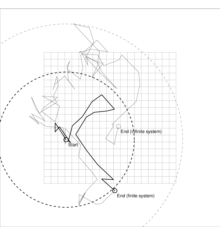
Figure 10: Example of 2-D random walk (or classical diffusion) in a finite system size lattice grid (trajectory with thick solid linestyle) and in an infinite system without boundaries (trajectory with thin solid linestyle). Both travel paths start at the same location, but end at a different location, either at the system boundary or outside of the finite system. The gyration radii of the two random walks are indicated with circles in dashed linestyle, differing by a factor of about two.

We may ask why flare durations (Fig. 3) do not show power laws extending over 3-5 decades as we find for peak fluxes and fluences (Fig. 2). We note that the inertial range with straight power law behavior is only 1-2 decades in size distributions of event durations, which makes it harder to separate it from the flattening at the lower end ($x\lower 1.72218pt\hbox{$\;\buildrel<\over{\scriptstyle\sim}\;$}x_{0}$) and the exponential cutoff at the upper end ($x\lower 1.72218pt\hbox{$\;\buildrel>\over{\scriptstyle\sim}\;$}x_{3}$). However, at this time it is not entirely understood why event durations have a pronounced exponential cutoff (Fig. 3), in contrast to event peak rates and fluences (Fig. 2). It appears that finite system-size effects are different in the time domain (e.g., flare durations) and in the spatial domain (see Fig. 10 and Appendix B).

3.4 Stellar Flare Finite Energy Limits

The size distribution of stellar flares according to the entire KEPLER (Borucki et al. 2010) flare event catalog (Davenport 2016; Yang and Liu 2019) includes a total of 162,264 flare events from different stars (normalized to the same stellar distance) and is shown in Fig. (4). This size distribution describes the largest available solar and stellar flare data set and extends over more than 4 decades, and thus can be modeled with much higher statistical accuracy than even the solar data sets (Fig. 2). The size distribution of the KEPLER flare luminosities has a power law slope of $\alpha_{F}=1.813\pm 0.004$, which is similar to the hard X-ray fluxes of solar flares (with $\alpha_{F}=1.79\pm 0.06$, averaged from Fig. (2a, 2b, 2c)). It is gratifying to find similar power law slopes for solar and stellar flare fluxes, which can be interpreted in terms of an identical physical process operating in both cases (such as the magnetic reconnection process).

The size distribution of stellar flare luminosities observed by KEPLER is best fitted with the extreme event model (EM), exhibiting a goodness-of-fit of $\chi=1.48$ (Fig. 4): The inertial range $[x_{0}=7\times 10^{33},x_{3}=1.5\times 10^{37}]$ erg is bracketing the power law part, over which our model fits apply. Some exponential cutoff around $x_{3}=q_{exp}x_{2}=0.04\ x_{2}\approx 1.5\times 10^{37}$ erg indicates finite system-size behavior, and the upper range range $[x_{0},x_{2}]$ (with the maximum size value at $x_{2}=4\times 10^{38}$ erg) indicates extreme events beyond the exponential cutoff, making up for a fraction of $q_{pow}=0.11$. It appears that 11% of the flare sizes belong to a group of high-energy flare events with extreme energies of $x\lower 1.72218pt\hbox{$\;\buildrel<\over{\scriptstyle\sim}\;$}x_{3}$, while the remaining 89% of the flares constitute a different group with low-energy events.

3.5 Stellar Spectral Types

Since the entire KEPLER flare catalog contains at least 6 different stellar spectral types (Davenport 2016; Yang and Liu 2019), it is of interest to study which spectral types produce the most extreme events and whether finite system-size effects occur that give us some stellar diagnostics. For instance, is the depth of the stellar convection zone related to the finite system-size inferred from size distributions?

We make use of the stellar spectral type classification of the KEPLER stellar flare catalog (A, F, G, K, M, Giants), for which the size distributions and power law fits are presented in Fig. 3 of Yang and Liu (2009), which is reproduced in Fig. 5 here. A list of the power law slopes $\alpha$ obtained by Yang and Liu (2009), with power law slopes $\alpha_{P},\alpha_{F},\alpha_{E}$ of our three models and the mean values (of the 3 models) are provided in Table 2. The agreement of the power law slopes $\alpha$ between the two studies is largely compatible: The differences are generally small, 14% for F-type stars, 9% for G-type, 1% for K-type, 16% for M-type, 5% for Giants, except for A-type stars (with a difference of 32%). We attribute this discrepancy of the power law slope in A-type stars ($\alpha=1.12\pm 0.08$ according to Yang and Liu (2009) versus $\alpha=1.65\pm 0.07$ in Fig. 5 here) to a flawed fit by an inadequate choice of the fitting range, which nullifies the claim of Yang and Liu (2009) that A-type stellar flares are produced by a different physical mechanism. The model fits shown in Fig. 5 exhibit a straight power law for K-type stars only (Fig. 5d), which shows also the best agreement (1%) between the two studies. All other spectral types exhibit significant deviations from straight power laws, which explains the discrepancies between the power law fits of Yang and Liu (2009) and our model fits. While arbitrary inertial ranges $[x_{0},x_{2}]$ have been used in the past to fit a power law, which is ill-defined in the absence of straight power laws, we recommend to use the Pareto distribution model (PM) (Eq. 3) to accomodate for incomplete sampling of small events, or more adequately, the model with finite system-size effects (FM; Eq. 4), and the model of extreme events (EM; Eq. 5). The goodness-of-fit $\chi\lower 1.72218pt\hbox{$\;\buildrel<\over{\scriptstyle\sim}\;$}2$ of these models is found to be acceptable for all stellar spectral types (Fig. 5).

We show a synopsis of the flare energy size distributions for the 6 spectral types of stellar flares, juxtaposed with the size distributions of all stellar and solar flare events in Fig. 6. This diagram demonstrates that incomplete sampling occurs up to energies of $E\lower 1.72218pt\hbox{$\;\buildrel<\over{\scriptstyle\sim}\;$}10^{35}$ erg, while the power law-like inertial ranges are confined to $E\approx 10^{35}-10^{37}$ erg. The most energetic flare events occur on Giant stars in the energy range of $E\approx 10^{37}-10^{38}$ erg, perhaps capped by extreme events at energies of $E\approx(1-5)\times 10^{38}$ erg. This upper limit is slightly higher than derived from sparse statistics of stellar flares ($E\lower 1.72218pt\hbox{$\;\buildrel<\over{\scriptstyle\sim}\;$}10^{37}$ erg) obtained before the KEPLER mission (see Fig. 3 in Schrijver et al. 2012).

We find that the median or the maximum flare energy $E_{max}$ in each stellar spectral type is related to the size of the star, based on the mean or maximum of the stellar radius $R/R_{\odot}$ (Fig. 7), defined by the Hertzsprung-Russell diagram of the Harvard spectral classification of main sequence and giant stars:

Giants, O-types $R\geq 6.6R_{\odot}$,

B-types $R=1.8-6.6R_{\odot}$,

A-types $R=1.4-1.8R_{\odot}$,

F-types $R=1.15-1.4R_{\odot}$,

G-types $R=0.96-1.15R_{\odot}$,

K-types $R=0.7-0.96R_{\odot}$,

M-types $R\leq 0.7R_{\odot}$.

We show this relationship for the median flare energy $E_{med}$ (diamonds) in Fig. 7, as well as for the maximum flare energy $E_{max}$ (crosses in Fig. 7), sampled from the size distributions of the KEPLER data (Fig. 6). This relationship supports the notion that the maximum flare energy $E_{max}$ scales with the spatial size (or stellar radius $R$), stellar surface area, or vertical depth of the stellar convection zone. In Fig. 7 we show also the relationship $E\propto(R^{2}+R_{M}^{2})$, which expresses that the stellar area $A=\pi R^{2}$ is an upper limit of the flare energy for Giants and A-type stars (since $R>R_{M}$), while M, K, F, G-type stars have flare energies with a lower limit at $R_{M}=0.7R_{\odot}$ (since $R<R_{M}$), possibly indicating a lower limit of the emission from the stellar corona, besides the chromospheric emission. Consequently we can associate the largest flare energies in the stellar flare size distribution with the finite system-size limit.

4 Conclusions

Occurrence frequency distributions (or size distributions) come in all shapes and sizes. The most common case is the power law function, which is easily to recognize by its straight line in a log(Number)-log(Size) representation, but one finds curved functions also that exhibit significant deviations from straight power laws and thus require refined models that can accomodate incomplete sampling, instrumental sensitivity limitations, event-unrelated background noise, truncation bias, finite system-size effects, and outliers of extreme events, possibly caused by multiple physical mechanisms, rather than a singular power law function produced by a classical SOC model. In order to illustrate the meaning of finite system-size effects in the context of SOC models see also APPENDIX B and Fig. 10. In this study we focus on the existence or absence of finite system-size effects, which requires large statistics with $n_{ev}\lower 1.72218pt\hbox{$\;\buildrel>\over{\scriptstyle\sim}\;$}10^{4}$ events per sample. We apply our data analysis to solar and stellar data sets, as well as to other empirical “real-world” data sets of interest to our human population (Appendix B). Our conclusions are summarized in the following.

1. We define 3 generalized power-law functions (Fig. 1): (i) the Pareto distribution that shows a flattening at the lower end due to incomplete sampling, and a straight power law at the upper end model (PM); (ii) the Pareto distribution with an exponentially dropping cutoff at the upper end that is caused by finite system-size effects (FM); and (iii) an additional power law component that extends above the exponential cutoff, caused by outlier events that are also called “Dragon-King” extreme events model (EM). We find that each of the 3 model functions can fit most of the observed 24 size distributions analyzed here with a goodness-of-fit of $\chi\lower 1.72218pt\hbox{$\;\buildrel<\over{\scriptstyle\sim}\;$}2$. This quantitative result is superior to previous straight power law fits, where (i) arbitrary (inertial) fitting ranges are used, (ii) power laws are ill-defined for curved size distributions, and (iii) no goodness-of-fit is specified.

2. We re-visit solar flare size distributions of the hard X-ray peak flux, the hard X-ray fluence, and flare durations (Figs. 2, 3). We corroborate previous findings that the peak fluxes and the fluences can be well fitted by Pareto distributions, with no sign of finite system-size effects at the upper end, indicating that larger super-flares are possible above the currently observed maximum size limit of $L\lower 1.72218pt\hbox{$\;\buildrel<\over{\scriptstyle\sim}\;$}200$ Mm. For flare durations we find that the best fits display an exponential cutoff at the upper end of $T_{2}\lower 1.72218pt\hbox{$\;\buildrel<\over{\scriptstyle\sim}\;$}6$ hrs, which suggests that solar flares cannot last longer in a coherent way. Size distributions of flare durations show no straight power law part, partially because of relatively smaller inertial ranges.

3. The KEPLER mission provides the largest statistics ($n_{ev}\approx 2.6\times 10^{5}$) of stellar flare energy size distributions, and thus facilitates the most detailed modeling of size distributions (Fig. 4). For the total of all KEPLER observed flares we find an approximate inertial range of $E\approx 10^{34}-10^{37}$ erg, a finite system-size range of $E\approx 10^{37}-10^{38}$ erg, and extreme events at $E\approx(1-5)\times 10^{38}$ erg. For smaller subsets of KEPLER data (e.g., Fig. 5), the detection of finite system-size effects is less feasible).

4. Subdividing the KEPLER flares into 6 stellar spectral types (Figs. 5,6) we find that the maximum flare energy $E_{max}$ in each stellar spectral type is related to the stellar radius $R/R_{\odot}$ (Fig. 7), based on the mean stellar radius defined by the Hertzsprung-Russell diagram of the Harvard spectral classification. This relationship supports the notion that the maximum flare energy may scale also with the vertical depth $z$ of the stellar convection zone, based on a convection cell geometry with compatible vertical and horizontal sizes, $z\approx 2R$. Consequently we expect that the stellar surface area $(4\pi R^{2})$ represents a finite system-size limit for flare energies in every stellar spectral type.

This study demonstrates that we can extract a large amount of new knowledge from model fitting of power law-like size distribution functions, sampled from a host of interdisciplinary data sets, pertaining to nonlinear energy dissipation events in SOC models. Although power law distributions are considered as the hallmark of SOC models (Bak et al. 1987, 1988; Aschwanden 2011; Aschwanden et al. 2016), a large number of pertaining data sets exhibit significant deviations from straight power laws, which justifies the eloquent criticism of Stumpf and Porter (2012). We have demonstrated here that refined modifications of power law-like functions, such as Pareto distribution functions, exponential cutoff functions, and dual (or multiple) power law functions are essential for more accurate fitting of observed size distributions. Future work may focus on finite system-size effects in solar and stellar flares, which may provide new knowledge on stellar convection and dynamos.

APPENDIX A: Finite System-Size Effects in Empirical Data

In the spirit of interdisciplinary research we fit our power law-like size distribution functions to 8 empirical data sets compiled by Clauset et al. (2009). Four out of these 8 cases show mostly Pareto distributions with a straight power law function all the way to the upper end of the size distribution (Fig. 8), covering information technology (word frequencies, surnames, and weblinks), as well as geophysics (Earth quakes). Another four data sets (Fig. 9) exhibit clear deviations from straight power laws, such as wildfires and human activities (city sizes, blackouts, terrorism statistics). Our size distribution models FM and EM indicate some sort of finite system-size effects, either in form of an exponential cutoff (see wildfires in Fig. 9b), or in form of a secondary power law component of extreme events beyond the cutoff (see city sizes, blackouts, terrorism in Fig. 9). The two power law components in the size distribution may indicate some duality of scales: wildfires may be subdivided into natural (e.g., by lightning) and human-induced fires (Krenn and Hergarten 2009); city sizes may be subdivided into two groups, depending on whether suburban agglomerations are merged with urban areas or not. The Zipf law does not fit as well with the data when using a traditional administrative definition of cities (Veneri 2013). Blackouts may be subdivided depending on whether a detected blackout produces a continent-wide ripple (cascading) or not (Shuvro et al. 2018). Acts of terrorism may have different statistics, depending on whether they are organized for economic causes, or for political causes (Kirk 1983). The identification of such dual behavior could give us a deeper understaning of complex size distribution functions that show significant deviations from ideal power laws.

APPENDIX B: Finite System-Size Effects in SOC

All known SOC systems have a finite system size. For instance, solar and stellar flares are limited by their finite solar or stellar surface area. Earth quakes or wild fires are ultimately bound by the Earth’s continents, etc. In the original sandpile model (Bak et al. 1987, 1988), upper limits on avalanche sizes are given by the geometric size of lattice 1-D, 2-D, or 3-D grids. The largest events span the distance from the central region to the remote boundaries of a sandpile. We illustrate the phenomenon of finite-size effects in Fig. 10. In the fractal-diffusive SOC model of a slowly-driven SOC system (Aschwanden 2012), the centroid of an avalanche propagates according to a random walk within the boundaries of a finite lattice grid and stops at the edge of the lattice grid (thick solid linestyle in Fig. 10), while the itinerary can cross the lattice boundaries, return to the inside area of the lattice, or even cross the boundaries multiple times (thin solid linestyle in Fig. 10), performing a random walk pattern. The radial extent of the avalanche is also called radius of gyration (Charbonneau et al. 2001), which obviously can have hugely different values for finite or infinite systems. Numerical simulations of avalanches with finite system size effects have been carried out in a number of studies (Pruessner 2012), which mostly demonstrated that the size distribution can be approximated with an exponential cutoff function (Eq. 4). Alternatively, some simulations show an additional bump near the exponential cutoff (see p. 33 in Pruessner 2012).

Acknowledgements: We acknowledge helpful comments from the Editor (Manolis Georgoulis) and an anonymous referee. Part of the work was supported by NASA contract NNG04EA00C of the SDO/AIA instrument and NNG09FA40C of the IRIS instrument.

References

Aschwanden, M.J. and Alexander, D. 2001, Flare Plasma Cooling from 30 MK down to 1 MK modeled from Yohkoh, GOES, and TRACE observations during the Bastille-Day Event (2000 July 14) SoPh 204, 91-121.

Aschwanden, M.J. 2011 Self-Organized Criticality in Astrophysics. The Statistics of Nonlinear Processes in the Universe, ISBN 978-3-642-15000-5, Springer-Praxis: New York, 416p.

Aschwanden, M.J. 2011, The state of self-organized criticality of the Sun during the last three solar cycles, SoPh 274:99-117.

Aschwanden, M.J. 2012, A statistical fractal-diffusive avalanche model of a slowly-driven self-organized criticality system A&A 539:A2.

Aschwanden, M.J. and Freeland, S.M. 2012, Automated solar flare statistics in soft X-rays over 37 years of GOES observations: The invariancxe of SOC during 3 solar cycles, ApJ 754:112.

Aschwanden, M.J. 2015, Thresholded power law size distributions of instabilities in astrophysics, ApJ 814:19.

Aschwanden, M.J. 2016, 25 Years of SOC: Solar and astrophysics, SSRv 198:47.

Aschwanden, M.J. 2019, Self-organized criticality in solar and stellar flares: Are extreme events scale-free ? ApJ 880, 105.

Aschwanden, M.J. 2020, Global energetics of solar flares. XII. Energy scaling laws, ApJ 903:23.

Bak, P., Tang, C., and Wiesenfeld, K. 1987, Self-organized criticality - An explanation of 1/f noise, Physical Review Lett. 59/27, 381-384.

Bak, P., Tang, C., and Wiesenfeld, K. 1988, Self-organized criticality, Physical Rev. A 38/1, 364-374.

Charbonneau, P., McIntosh, S.W., Liu, H.L., and Bogdan,T.J. 2001, Avalanche models for solar flares, SoPh 203, 321.

Clauset, A., Shalizi, C.R., and Newman, M.E.J. 2009, Power-law distributions in empirical data, SIAM Review 51/4, 661-703.

Borucki, W.J., Koch, D., Basri, G. et al. 2010, Kepler planet-detection mission: Introduction and first results Science 327, 977.

Davenport, J.R. 2016, The Kepler Catalog of stellar flares, ApJ 829:23.

Drossel B. and Schwabl F. 1992, Self-organized critical forest-fire model. Phys. Rev. Lett 69:1629-1632.

Hergarten S. 2013, Wildfires and the Forest-Fire Model, in Self-Organized Criticality Systems (ed., M.J. Aschwanden), Open Academic Press, www.openacademicpress.de

Hill B.M. 1975, Annals of Statistics 3, 1163.

Hosking, J.M.R. and Wallis, J.R. 1987, Technometrics 29, 339.

Kirk, R.M. 1983, Political terrorism and the size of government: A positive institutional analysis of violent political activity, Public Choice 40, 41–52, https://doi.org/10.1007/BF00174995

Krenn, R. and Hergarten, S. 2009, Cellular automaton modelling of lightening-induced and man-made forest fires, Natural Hazards and Earth System Sciences 9:1743-1748.

Lomax, K.S. 1954, , J. Am. Stat. Assoc. 49, 847.

Malamud, B.D., Morein, G., and Turcotte, D.L. 1998, Science 281:1840-1842.

Pruessner, G. 2012, Self-organised criticality. Theory, models and characterisation, Cambridge University Press, Cambridge.

Schrijver, C.J., Beer, J., Baltensperger, U. et al. 2012, Estimating the frequency of extremely energetic solar events, based on solar, stellar, lunar, and terrestrial records, JGRA 117, A8, CiteID A08103.

Shuvro, R., Das, P., Wang, Z., Rahnamay-Naeini, M., and Hayat, M. 2018. Impact of Initial Stressor(s) on Cascading Failures in Power Grid. DOI 10.1109/NAPS.2018.8600585

Sornette, D. 2009, Dragon-King, Black-Swans and the prediction of crises, J. Terraspace Science and Engineering, 2, 1

Sornette, D. and Ouillon, G. 2012, Dragon-Kings: Mechanisms, statistical methods and empirical evidence, EPJST 205, 1

Stumpf, M.P.H. and Porter, M.A. 2012, Science 335, 665.

Taleb, N.N. (2007, 2010), The Black Swan: the impact of the highly improbable (2nd ed.). London: Penguin, ISBN 978-0-14103459-1.

Veneri P. 2013, On City Size Distribution: Evidence from OECD Functional Urban Areas, OECD Regional Development Working Papers 2013/27, https://dx.doi.org/10.1787/5k3tt100wf7j-en

Yang, H. and Liu, J. 2019, The flare catalog and the flare activity in the Kepler mission, ApJSS 241:1

Zinck, R.D. and Grimm, V. 2008, Open Ecol J 1:8-13, DOI 10.2174/1874213000801010008.

Table 1: Observed phenomena with power law slopes, goodness-of-fit, and models (PM = Pareto Distribution model, FM = Finite System-Size model, EM = Finite System-Size and extreme event model).

Observable	Number	Background	Power law	Goodness	Model
	of events	level	slope	$\chi^{2}$
Peak flux HXRBS	11,352	1	$1.75\pm 0.02$	0.88	EM
Peak flux BATSE	7,245	1	$1.76\pm 0.02$	1.87	EM
Peak flux RHESSI	7,998	1	$1.85\pm 0.02$	1.41	PM
Counts HXRBS	11,550	1	$1.57\pm 0.01$	1.52	PM
Counts BATSE	3,425	1	$1.65\pm 0.03$	0.90	PM
Counts RHESSI	11,549	1	$1.74\pm 0.02$	1.51	PM
Duration HXRBS	11,549	0	$1.81\pm 0.02$	1.81	EM
Duration BATSE	7,243	0	$1.99\pm 0.02$	1.04	FM
Duration RHESSI	11,525	0	$1.90\pm 0.02$	1.40	FM
Kepler (catalog)	162,264	1	$1.813\pm 0.002$	1.45	EM
Words	9,695	1	$2.12\pm 0.02$	1.85	EM
Surnames	2,753	1	$2.58\pm 0.05$	1.72	PM
Weblinks	8,658	1	$1.49\pm 0.02$	1.94	PM
Earth quakes	17,452	1	$1.71\pm 0.01$	1.98	EM
City sizes	19,447	1	$1.59\pm 0.01$	1.57	EM
Wildfires	56,052	1	$1.77\pm 0.01$	1.56	FM
Blackouts	213	1	$1.35\pm 0.10$	0.73	EM
Terrorisms	4,303	1	$2.64\pm 0.04$	1.26	FM

Table 2: Model fitting of the power law slope of the size distributions of stellar flares observed with KEPLER for three models (PM = Pareto Distribution model, FM = Finite System-Size model, EM = Finite System-Size and extreme event model), separately sampled for six different stellar spectral types (A, F, G, K, M, and Giants), and compared with the previously published results of Yang and Liu (2009).

Spectral	Number	Power law	Power law	Power law	Power law	Power law
type	of events	Yang and Liu (2009)	PM	FM	EM	average
		$\alpha$	$\alpha_{PM}$	$\alpha_{PM}$	$\alpha_{EM}$	$\alpha_{avg}$
A-type	583	$1.12\pm 0.08$	$1.65\pm 0.07$	$1.65\pm 0.07$	$1.65\pm 0.07$	$1.65\pm 0.00$
F-type	8869	$2.11\pm 0.09$	$1.96\pm 0.02$	$1.80\pm 0.02$	$1.79\pm 0.02$	$1.85\pm 0.09$
G-type	55,259	$1.96\pm 0.04$	$1.85\pm 0.01$	$1.80\pm 0.01$	$1.72\pm 0.01$	$1.79\pm 0.06$
K-type	47,112	$1.78\pm 0.02$	$1.69\pm 0.01$	$1.67\pm 0.01$	$2.03\pm 0.01$	$1.80\pm 0.20$
M-type	50,439	$2.13\pm 0.05$	$1.83\pm 0.01$	$1.83\pm 0.01$	$1.86\pm 0.01$	$1.84\pm 0.02$
Giants	6,496	$1.90\pm 0.10$	$2.39\pm 0.03$	$1.80\pm 0.02$	$1.80\pm 0.02$	$2.00\pm 0.34$

Figure 1: Synopsis of three power law models: (PM) = Pareto distribution model $[x_{1},x_{0}]$, (EM) = Extreme events model $[x_{3},x_{2}$], and (FM) = Finite system-size model $[\lower 1.72218pt\hbox{$\;\buildrel>\over{\scriptstyle\sim}\;$}x_{3}]$. The inertial range covers $[\lower 1.72218pt\hbox{$\;\buildrel>\over{\scriptstyle\sim}\;$}x_{0},\lower 1.72218pt\hbox{$\;\buildrel<\over{\scriptstyle\sim}\;$}x_{3}$]. The data used here are from the Kepler flare catalog, see also Table 1 and Fig. 4.

Figure 2: Differential occurrence size distributions of solar hard X-ray peak fluxes (left panels) and total counts (right panels), observed with three different instruments (HXRBS, BATSE, RHESSI) (binned histograms) and fitted with the model functions (solid curves) over an inertial range of $[x_{0},x_{2}]$. For comparison, the power law slope is indicated with a dotted line.

Figure 3: Differential occurrence size distributions of solar flare durations, observed with three different instruments (HXRBS, BATSE, RHESSI) (binned histograms) and fitted with the model functions (solid curves) over an inertial range of $[x_{0},x_{2}]$. The size $x_{3}$ refers to the finite system-size model.

Figure 4: Differential occurrence size distributions of stellar flare energy observed with KEPLER (binned histograms) and fitted with the model function (solid curve) over an inertial range of $[x_{0},x_{3}]$. The size $x_{3}$ refers to the finite system-size model. The power law slope is indicated with a dotted diagonal.

Figure 5: Size distributions of stellar flare energies observed with KEPLER in six groups of different spectral types (histograms), reproduced from Fig. 3 in Yang and Liu (2019). The size distributions are fitted with our model EM for extreme events (thick solid curves). Note the deviations from straight power laws.

Figure 6: Composite size distribution of stellar flares (diamonds), containing six groups with different stellar spectral types (A, F, G, K, M, Giants). For comparison we show also the size distributions of solar (asterisks) and all stellar flares (diamonds) combined (thick solid lines).

Figure 7: Observed relationship between the maximum (curve with crosses) and median (curve with diamonds) flare energies $E_{max}$ and the stellar radius in units of solar radii, $R/R_{\odot}$, for 6 different stellar spectral types. The thin curves depict the relationship $E\propto(R^{2}+R_{M}^{2})$, where $R_{M}=0.7R_{\odot}$ represents the lower limit of M dwarf stars.

Figure 8: Differential occurrence size distributions of empirical data sets compiled by Clauset et al. (2009) (binned histograms) and fitted with the model functions (solid curves) over an inertial range of $[x_{0},x_{2}]$.

Figure 9: Differential occurrence size distributions of empirical data compiled by Clauset et al. (2009) (binned histograms) and fitted with the model functions (solid curves) over an inertial range of $[x_{0},x_{2}]$.