Elliptical rotation of cavity amplitude in ultrastrong waveguide QED

Abstract

We investigate optical response of a linear waveguide quantum electrodynamics (QED) system, namely, an optical cavity coupled to a waveguide. Our analysis is based on exact diagonalization of the overall Hamiltonian and is therefore rigorous even in the ultrastrong coupling regime of waveguide QED. Owing to the counter-rotating terms in the cavity-waveguide coupling, the motion of cavity amplitude in the phase space is elliptical in general. Such elliptical motion becomes remarkable in the ultrastrong coupling regime due to the large Lamb shift comparable to the bare cavity frequency. We also reveal that such elliptical motion does not propagate into the output field and present an analytic form of the reflection coefficient that is asymmetric with respect to the resonance frequency.

I introduction

Cavity quantum electrodynamics (QED) deals with the interaction between a single atom and a discretized photon mode confined in a resonator, which is the simplest embodiment of quantum light-matter interaction. The cavity QED systems have been realized in various physical platforms: just to cite a few, single atoms coupled to an optical cavity, a semiconductor quantum dot in a photonic-crystal cavity, and a superconducting qubit coupled to a transmission-line resonator. Interestingly, regardless of its physical platform, a cavity QED system is characterized by several universal parameters, such as $\omega_{a}$ and $\omega_{c}$ (atom and cavity frequencies), $g$ (atom-photon coupling), $\kappa$ (cavity decay rate), and $\gamma$ (atomic decay rate into environments). In the history of cavity QED, extensive efforts have been made to reach the strong-coupling regime ($g>\kappa,\gamma$), where the vacuum Rabi oscillation and splitting become observable sc1 ; sc2 ; sc3 ; sc4 . In usual strong-coupling systems, the coupling is still by far smaller than the resonance frequencies of the atom and cavity. Recently, attainments of the ultrastrong-coupling ($g\gtrsim\omega_{a,c}/10$) and deep-strong-coupling ($g\gtrsim\omega_{a,c}$) regimes have been reported us1 ; us2 ; us3 ; us4 ; us5 ; deep1 ; deep2 . In such ultrastrong-coupling systems, the counter-rotating terms in the Hamiltonian, which do not conserve the total number of excitations and are usually negligible in the weakly coupled systems, result in several intriguing physical phenomena, such as the Bloch-Siegert shift BS1 ; BS2 , virtual photons in the ground state vp1 ; vp2 ; vp3 ; vp4 ; vp5 , and the number non-conserving optical processes such as multiphoton vacuum Rabi oscillation multi0 ; multi1 ; multi2 .

Waveguide QED deals with the interaction between a single atom and a one-dimensional continuum of photon modes, typically provided by a waveguide attached to the atom. The parameters to characterize waveguide QED systems are $\omega_{a}$, $\gamma_{e}$ (atomic decay rate into waveguide) and $\gamma_{i}$ (atomic decay rate into environments). The strong-coupling regime in waveguide QED is defined by $\gamma_{e}>\gamma_{i}$, namely, the condition that radiation from the atom is dominantly forwarded to the waveguide wQED1 ; wQED2 ; wQED3 ; wQED4 ; wQED5 ; wQED6 . This is reflected in spectroscopy as a strong suppression of transmission near the atomic resonance. Following the definitions in cavity QED, the ultra- and deep-strong waveguide QED should be defined as $\gamma_{e}\gtrsim\omega_{a}/10$ and $\gamma_{e}\gtrsim\omega_{a}$, respectively. The ultrastrong and deep-strong regimes of waveguide QED have already been reached using a superconducting qubit usQED1 ; usQED2 . Theoretically, up to the usual strong-coupling regime, perturbative treatment of dissipation based on the rotating-wave and Born-Markov approximations provides convenient and powerful theoretical tools, such as the Lindblad master equation and the input-output formalism th0a ; th0b . However, this is not the case in highly dissipative regimes, and rigorous numerical methods are actively developed th1 ; th2 ; th3 ; th4 .

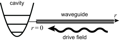
Figure 1: Schematic of a cavity-waveguide system. A cavity is coupled to a semi-infinite waveguide, through which a monochromatic drive field is applied. The $r<0$ ($r>0$) region in the waveguide corresponds to the input (output) port.

In this study, we investigate a linear waveguide QED setup, namely, a harmonic oscillator coupled to a waveguide, and investigate its optical response to a classical drive field applied through this waveguide. A merit of this system is that the overall Hamiltonian is diagonalizable by the Fano’s method Fano1 ; Fano2 ; Fano3 and rigorous optical response is accessible even for highly dissipative situations. We report an elliptic motion of the oscillator in the phase space, which occurs, in principle, even in the usual waveguide QED setups but becomes remarkable in the ultrastrong-coupling regime due to the large Lamb shift. However, in contrast with the intuition provided by the input-output theory, such elliptic motion does not propagate into the waveguide. We also obtain an analytic formula of the reflection/transmission coefficient, which is asymmetric with respect to the renormalized cavity frequency. We hope that the rigorous optical response presented here would be useful for developing theoretical tools applicable to highly dissipative cavity and waveguide QEDs.

II theoretical model

II.1 Hamiltonian

In a setup considered in this study (Fig. 1), a cavity is coupled to a semi-infinite waveguide and a monochromatic drive field is applied through this waveguide. In the natural units of $\hbar=v=1$, where $v$ is the photon velocity in the waveguide, the Hamiltonian of the overall system is given by

$$\hat{H} = \omega_{b}\hat{b}^{{\dagger}}\hat{b}+\int_{0}^{\infty}dk\left[k\hat{c}_{k}^{{\dagger}}\hat{c}_{k}+\xi_{k}(\hat{b}^{{\dagger}}+\hat{b})(\hat{c}_{k}^{{\dagger}}+\hat{c}_{k})\right],$$ (1)

where $\omega_{b}$ is the bare cavity frequency, and $\hat{b}$ and $\hat{c}_{k}$ are the annihilation operators of the cavity mode and the waveguide mode with wave number $k$, respectively, satisfying the bosonic commutation relations, $[\hat{b},\hat{b}^{{\dagger}}]=1$ and $[\hat{c}_{k},\hat{c}^{{\dagger}}_{k^{\prime}}]=\delta(k-k^{\prime})$. The cavity-waveguide coupling $\xi_{k}$ is a real function of $k$. In this study, in order that the Fano diagonalization is applicable, we assume the following conditions on $\xi_{k}$ Fano2 : (i) $\xi_{k}$ is nonzero for $k>0$, (ii) $\xi^{2}_{k}$ is an odd function of $k$, namely, $\xi^{2}_{-k}=-\xi^{2}_{k}$, and (iii) the coupling is weak enough to satisfy

$$\int_{0}^{\infty}dk\ \xi^{2}_{k}/k < \omega_{b}/4.$$ (2)

II.2 Drude-form coupling

To be more concrete, we employ a Drude-form for the cavity-waveguide coupling,

$$\xi_{k}^{2} = C\frac{k}{k^{2}+\omega_{x}^{2}},$$ (3)

where $C$ is a constant and $\omega_{x}$ is the cutoff frequency. We assume $\omega_{x}\gg\omega_{b}$ so that the coupling is Ohmic ($\propto k$) near the cavity resonance. We set $\omega_{x}=5~{}\omega_{b}$ hereafter. We denote the radiative decay rate of the cavity mode into the waveguide by $\kappa$. By naively applying the Fermi golden rule, we obtain $\kappa=2\pi\xi_{\omega_{b}}^{2}$. Therefore, we set the constant $C$ as

$$C = \frac{\kappa(\omega_{b}^{2}+\omega_{x}^{2})}{2\pi\omega_{b}}.$$ (4)

In this paper, we employ a dimensionless quantity $\kappa/\omega_{b}$ as a measure of the strength of the cavity-waveguide coupling.

II.3 Renormalization of frequency and decay rate

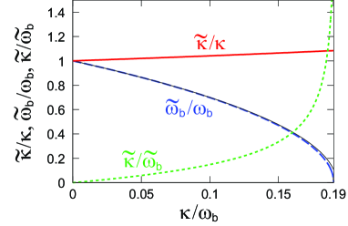
Figure 2: Dependences of the cavity decay rate ($\widetilde{\kappa}/\kappa$, solid) and resonance frequency ($\widetilde{\omega}_{b}/\omega_{b}$, dashed) on the cavity-waveguide coupling, $\kappa/\omega_{b}$. Their ratio, $\widetilde{\kappa}/\widetilde{\omega}_{b}$, is plotted by a dotted line. The ultrastrong coupling ($\widetilde{\kappa}/\widetilde{\omega}_{b}>0.1$) is attained for $\kappa/\omega_{b}>0.076$ and the deep-strong coupling ($\widetilde{\kappa}/\widetilde{\omega}_{b}>1$) is attained for $\kappa/\omega_{b}>0.183$. An alternative expression of the renormalized frequency, Eq. (44), is also shown (thin solid).

Since the Fermi golden rule is in principle valid only for a weak cavity-waveguide coupling, $\kappa$ may deviate from the actual decay rate $\widetilde{\kappa}$, particularly for a stronger coupling. Furthermore, the resonance frequency $\omega_{b}$ also acquires a Lamb shift and takes a renormalized value $\widetilde{\omega}_{b}$. As we observe later in Sec. III.2, $\widetilde{\omega}_{b}$ and $\widetilde{\kappa}$ are identified as

$$\widetilde{\omega}_{b} = \mathrm{Re}(\lambda_{1}),$$ (5)

$$\widetilde{\kappa} = 2\ \mathrm{Im}(\lambda_{1}),$$ (6)

where $\lambda_{1}$ is a complex cavity frequency, which is a solution of the cubic equation (23) in the first quadrant (Fig. 3).

From Eq. (2), we have $\kappa/\omega_{b}<\omega_{b}\omega_{x}/(\omega_{b}^{2}+\omega_{x}^{2})$. This inequality sets an upper bound for the coupling strength: $\kappa/\omega_{b}<0.192$ for $\omega_{x}=5\omega_{b}$. However, as we discuss in Sec. III.2, from the condition that the renormalized frequency $\widetilde{\omega}_{b}$ is positive, we have a more strict upper bound, $\kappa/\omega_{b}<0.190$.

In Fig. 2, we plot the dependences of $\widetilde{\omega}_{b}$ and $\widetilde{\kappa}$ on $\kappa/\omega_{b}$. We observe that, beyond the perturbative regime of $\kappa/\omega_{b}\ll 1$, the agreement between $\widetilde{\kappa}$ and $\kappa$ is fairly good even for stronger coupling. In contrast, the renormalized cavity frequency decreases drastically as the coupling becomes stronger. As a result, not only the ultrastrong coupling regime ($\widetilde{\kappa}/\widetilde{\omega}_{b}>0.1$) but also the deep-strong coupling regime ($\widetilde{\kappa}/\widetilde{\omega}_{b}>1$) is attainable within this theoretical model.

II.4 Initial state vector

In this study, we investigate the optical response of a cavity driven by a monochromatic classical field applied through the waveguide (Fig. 1). The positively rotating part of drive amplitude is given by

$$E(r,t) = E_{d}e^{ik_{d}(r-t)},$$ (7)

where $E_{d}$ and $k_{d}$ are the complex amplitude and wavenumber/frequency of the drive, respectively. At the initial moment ($t=0$), we assume that the whole system is in the ground state expect the drive field in the waveguide, which is in a coherent state. The initial state vector is then written as

$$|\psi_{i}\rangle = \exp\left(\sqrt{2\pi}E_{d}\hat{c}_{k_{d}}^{{\dagger}}-\sqrt{2\pi}E^{*}_{d}\hat{c}_{k_{d}}\right)|vac\rangle,$$ (8)

where $|vac\rangle$ is the overall ground state.

The real-space representation $\widetilde{c}_{r}$ of the waveguide field operator is defined as the Fourier transform of $\hat{c}_{k}$,

$$\widetilde{c}_{r} = \frac{1}{\sqrt{2\pi}}\int_{0}^{\infty}dk\ e^{ikr}\hat{c}_{k}.$$ (9)

We can check that $\langle\widetilde{c}_{r}(0)\rangle\equiv\langle\psi_{i}|\widetilde{c}_{r}(0)|\psi_{i}\rangle=E(r,0)$. Strictly speaking, the real-space representation of the waveguide mode depends on the boundary condition of the waveguide at $r=0$. For example, for a closed boundary condition, the waveguide mode function takes the form of $f_{k}(r)=\sqrt{2/\pi}\sin(kr)=(ie^{-ikr}-ie^{ikr})/\sqrt{2\pi}$ norm . Therefore, we should add a phase factor $i$ ($-i$) for the input (output) port in Eq. (9), which accounts for the sign flip upon reflection at a mirror. However, we employ Eq. (9) as the real-space representation of waveguide modes for simplicity. This introduces no problem except for definition of the relative phase in the input and output ports.

III Diagonalization

III.1 General formula

The Hamiltonian [Eq. (1)] is bilinear in bosonic operators and can be diagonalized by the Fano’s method. When the cavity-waveguide coupling is weak enough to satisfy Eq. (2), we can rewrite the Hamiltonian as

$$\hat{H} = \int_{0}^{\infty}dk\ k\hat{d}_{k}^{{\dagger}}\hat{d}_{k},$$ (10)

where $\hat{d}_{k}$ is an eigenmode annihilation operator satisfying the bosonic commutation relation,

$$[\hat{d}_{k},\hat{d}_{k^{\prime}}^{\dagger}] = \delta(k-k^{\prime}).$$ (11)

$\hat{d}_{k}$ is given by linear combination of the original bosonic operators as

$$\hat{d}_{k} = \beta_{1}(k)\hat{b}+\beta_{2}(k)\hat{b}^{{\dagger}}+\int_{0}^{\infty}dq\left[\gamma_{1}(k,q)\hat{c}_{q}+\gamma_{2}(k,q)\hat{c}_{q}^{{\dagger}}\right],$$ (12)

where the coefficients are given by (see Appendix A for derivation)

$$\beta_{1}(k) = \frac{(k+\omega_{b})\xi_{k}}{k^{2}-\omega_{b}^{2}z(k)},$$ (13)

$$\beta_{2}(k) = \frac{(k-\omega_{b})\xi_{k}}{k^{2}-\omega_{b}^{2}z(k)},$$ (14)

$$\gamma_{1}(k,q) = \delta(k-q)+\widetilde{\gamma}_{1}(k,q),$$ (15)

$$\gamma_{2}(k,q) = \frac{2\omega_{b}\xi_{k}\xi_{q}}{(k+q)[k^{2}-\omega_{b}^{2}z(k)]},$$ (16)

where

$$\widetilde{\gamma}_{1}(k,q) = \frac{2\omega_{b}\xi_{k}\xi_{q}}{(k-q-i0)[k^{2}-\omega_{b}^{2}z(k)]},$$ (17)

and $z(k)$ is a dimensionless quantity representing the self-energy correction for the resonator frequency,

$$z(k) = 1+\frac{2}{\omega_{b}}\int_{-\infty}^{\infty}dq\frac{\xi_{q}^{2}}{k-q-i0}.$$ (18)

Inversely, the bare operators $\hat{b}$ and $\hat{c}_{k}$ are expressed in terms of the eigenoperators by

$$\hat{b} = \int_{0}^{\infty}dq[\beta_{1}^{*}(q)\hat{d}_{q}-\beta_{2}(q)\hat{d}_{q}^{{\dagger}}],$$ (19)

$$\hat{c}_{k} = \int_{0}^{\infty}dq[\gamma_{1}^{*}(q,k)\hat{d}_{q}-\gamma_{2}(q,k)\hat{d}_{q}^{{\dagger}}].$$ (20)

III.2 Specific results for Drude-form coupling

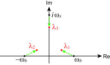
Figure 3: $\lambda_{1,2,3}$ on the complex plane. Arrows indicate the directions as the cavity-waveguide coupling $\kappa$ is increased.

When the cavity-waveguide coupling takes the Drude form [Eqs. (3) and (4)], $z(k)$ and $k^{2}-\omega_{b}^{2}z(k)$ are rewritten as follows,

$$z(k) = 1+\frac{2\pi iC}{\omega_{b}(k-i\omega_{x})},$$ (21)

$$k^{2}-\omega_{b}^{2}z(k) = \frac{(k-\lambda_{1})(k-\lambda_{2})(k-\lambda_{3})}{k-i\omega_{x}},$$ (22)

where $\lambda_{1,2,3}$ are the solutions of the following cubic equation for $k$,

$$k^{3}-i\omega_{x}k^{2}-\omega_{b}^{2}k+(i\omega_{x}\omega_{b}^{2}-2i\pi C\omega_{b}) = 0.$$ (23)

As shown in Fig. 3, $\lambda_{1}$ ($\lambda_{2}$) is on the first (seond) quadrant and $\lambda_{3}$ is on the positive imaginary axis. The real and imaginary parts of $\lambda_{1}$ correspond to the Lamb-shifted resonance frequency $\widetilde{\omega}_{b}$ and half of the decay rate $\widetilde{\kappa}/2$ [Eqs. (5) and (6)]. For reference, we present the perturbative solution of Eq. (23) with respect to the cavity-waveguide coupling $\kappa$. The zeroth-order solutions are $\lambda_{1}^{(0)}=\omega_{b}$, $\lambda_{2}^{(0)}=-\omega_{b}$, and $\lambda_{3}^{(0)}=i\omega_{x}$. Up to the first order in $\kappa$, the three solutions are given by $\lambda_{1}\approx(\omega_{b}-\kappa\omega_{x}/2\omega_{b})+i\kappa/2$, $\lambda_{2}\approx-(\omega_{b}-\kappa\omega_{x}/2\omega_{b})+i\kappa/2$, and $\lambda_{3}\approx i\omega_{x}-i\kappa$.

For an extremely strong coupling, $\lambda_{1}$ and $\lambda_{2}$ also become purely imaginary. The condition that the renormalized frequency $\widetilde{\omega}_{b}$ remain positive, in other words, $\lambda_{1}$ and $\lambda_{2}$ are not purely imaginary, is that $\kappa<[\omega_{b}^{2}\omega_{x}-f(\mu_{-})]/(\omega_{b}^{2}+\omega_{x}^{2})$, where $f(x)=x^{3}-\omega_{x}x^{2}+\omega_{b}^{2}x$ and $\mu_{-}$ is a smaller root of the $df/dx=0$, namely, $\mu_{-}=(\omega_{x}-\sqrt{\omega_{x}^{2}-3\omega_{b}^{2}})/3$. For $\omega_{x}=5~{}\omega_{b}$, this condition is $\kappa/\omega_{b}<0.190$.

IV optical response

IV.1 Cavity Amplitude

In this section, we investigate time evolution of the whole system from the initial state vector, Eq. (8). We first observe the amplitude of the cavity mode, $\langle\hat{b}(t)\rangle\equiv\langle\psi_{i}|\hat{b}(t)|\psi_{i}\rangle$. Since $\hat{d}_{k}$ is an eigenoperator of the Hamiltonian, $\hat{b}(t)$ is given, from Eq. (19), by

$$\hat{b}(t) = \int_{0}^{\infty}dq\left[e^{-iqt}\beta_{1}^{*}(q)\hat{d}_{q}-e^{iqt}\beta_{2}(q)\hat{d}^{{\dagger}}_{q}\right].$$ (24)

Furthermore, $|\psi_{i}\rangle$ is an eigenstate of $\hat{d}_{q}$ and satisfies

$$\hat{d}_{q}|\psi_{i}\rangle = \sqrt{2\pi}[E_{d}\gamma_{1}(q,k_{d})+E^{*}_{d}\gamma_{2}(q,k_{d})]|\psi_{i}\rangle.$$ (25)

From these results, $\langle\hat{b}(t)\rangle$ is given by

$$\langle\hat{b}(t)\rangle = \sqrt{2\pi}E_{d}\int_{0}^{\infty}dq\left[e^{-iqt}\beta_{1}^{*}(q)\gamma_{1}(q,k_{d})-e^{iqt}\beta_{2}(q)\gamma_{2}^{*}(q,k_{d})\right]$$ (26)

$$+ \sqrt{2\pi}E^{*}_{d}\int_{0}^{\infty}dq\left[e^{-iqt}\beta_{1}^{*}(q)\gamma_{2}(q,k_{d})-e^{iqt}\beta_{2}(q)\gamma_{1}^{*}(q,k_{d})\right].$$

This is divided into stationary and transient components as $\langle\hat{b}(t)\rangle=\langle\hat{b}(t)\rangle_{s}+\langle\hat{b}(t)\rangle_{t}$. The stationary component is given by

$$\langle\hat{b}(t)\rangle_{s} = \sqrt{2\pi}\beta_{1}^{*}(k_{d})E_{d}e^{-ik_{d}t}-\sqrt{2\pi}\beta_{2}(k_{d})E_{d}^{*}e^{ik_{d}t}.$$ (27)

The transient component is presented in Appendix B. Putting $E_{d}=|E_{d}|e^{i\theta_{d}}$, we have

$$\mathrm{Re}\langle\hat{b}(t)\rangle_{s} = \sqrt{8\pi}|E_{d}|\omega_{b}\xi_{k_{d}}\mathrm{Re}\left(\frac{e^{i(k_{d}t-\theta_{d})}}{k_{d}^{2}-\omega_{b}^{2}z(k_{d})}\right),$$ (28)

$$\mathrm{Im}\langle\hat{b}(t)\rangle_{s} = -\sqrt{8\pi}|E_{d}|k_{d}\xi_{k_{d}}\mathrm{Im}\left(\frac{e^{i(k_{d}t-\theta_{d})}}{k_{d}^{2}-\omega_{b}^{2}z(k_{d})}\right).$$ (29)

These equations indicate that the motion of the cavity amplitude $\langle\hat{b}(t)\rangle_{s}$ on the phase space is elliptical in general; the ratio of the vertical (imaginary) radius relative to the horizontal (real) radius is $k_{d}/\omega_{b}$, and thus depends on the drive frequency. However, such elliptical motion is not remarkable when the cavity-waveguide coupling $\kappa$ is small. For a small $\kappa$ case, strong optical response is obtained within a narrow frequency region around the renormalized cavity frequency $\widetilde{\omega}_{b}$, which is close to the bare frequency $\omega_{b}$. For example, when $\kappa/\omega_{b}=0.01$, the renormalized frequency amounts to $\widetilde{\omega}_{b}=0.975~{}\omega_{b}$ [Eq. (44)]. Therefore, the motion is almost circular for small $\kappa$, as we observe in Figs. 4 (a) and (c). In contrast, for a large $\kappa$ case, the motion on the phase space becomes highly elliptical, as we observe in Figs. 4 (b) and (d). This is due to the large frequency renormalization (Lamb shift). When $\kappa/\omega_{b}=0.15$, the renormalized frequency amounts to $\widetilde{\omega}_{b}=0.476~{}\omega_{b}$.

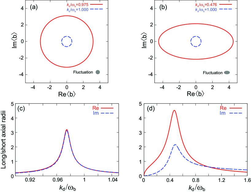
Figure 4: Elliptical motion of the cavity amplitude. (a) Trajectories on the phase space for $\kappa/\omega_{b}=0.01$. The drive frequency is set at the renormalized resonance $\widetilde{\omega}_{b}(=0.975~{}\omega_{b})$ (solid) and the bare resonance $\omega_{b}$ (dashed). The photon rate of the drive field is set at $|E_{d}|^{2}=2.5~{}\kappa$, at which the mean intra-cavity photon number is estimated to be $\langle\hat{b}^{{\dagger}}\hat{b}\rangle=4|E_{d}|^{2}/\kappa=10$ on resonance, following the input-output theory. The uncertainty ellipse is also shown. (b) The same plot as (a) for $\kappa/\omega_{b}=0.15$. The renormalized resonance is $\widetilde{\omega}_{b}=0.476~{}\omega_{b}$. (c) Dependence of the long (solid line) and short (dotted line) axial radii on the drive frequency $k_{d}$ for $\kappa/\omega_{b}=0.01$. (d) The same plot as (c) for $\kappa/\omega_{b}=0.15$.

IV.2 Quadrature Fluctuations

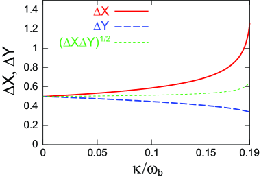
Figure 5: Quadrature fluctuations: $\Delta X$ (solid), $\Delta Y$ (dashed), and $\sqrt{\Delta X\Delta Y}$ (thin dotted). $\omega_{x}/\omega_{b}=5$.

Here, we investigate the quadrature fluctuations of the cavity mode. We define the $\hat{X}$ and $\hat{Y}$ quadratures by $\hat{X}=(\hat{b}+\hat{b}^{\dagger})/2$ and $\hat{Y}=-i(\hat{b}-\hat{b}^{\dagger})/2$, respectively, and their fluctuations by $\Delta X=\sqrt{\langle\hat{X}^{2}\rangle-\langle\hat{X}\rangle^{2}}$ and $\Delta Y=\sqrt{\langle\hat{Y}^{2}\rangle-\langle\hat{Y}\rangle^{2}}$, respectively, where $\langle\hat{O}\rangle=\langle\psi_{i}|\hat{O}|\psi_{i}\rangle$. From these definitions, we have

$$\Delta X = \frac{\sqrt{1+2\langle\hat{b}^{{\dagger}}(t),\hat{b}(t)\rangle+2\mathrm{Re}\langle\hat{b}(t),\hat{b}(t)\rangle}}{2},$$ (30)

$$\Delta Y = \frac{\sqrt{1+2\langle\hat{b}^{{\dagger}}(t),\hat{b}(t)\rangle-2\mathrm{Re}\langle\hat{b}(t),\hat{b}(t)\rangle}}{2},$$ (31)

where $\langle\hat{O},\hat{O}^{\prime}\rangle\equiv\langle\hat{O}\hat{O}^{\prime}\rangle-\langle\hat{O}\rangle\langle\hat{O}^{\prime}\rangle$. From Eqs. (24) and (25), we can confirm that both $\langle\hat{b}^{{\dagger}}(t),\hat{b}(t)\rangle$ and $\langle\hat{b}(t),\hat{b}(t)\rangle$ reduces to the following time-independent quantities,

$$\langle\hat{b}^{{\dagger}},\hat{b}\rangle = \int_{0}^{\infty}dq|\beta_{2}(q)|^{2},$$ (32)

$$\langle\hat{b},\hat{b}\rangle = -\int_{0}^{\infty}dq\beta_{1}^{*}(q)\beta_{2}(q),$$ (33)

and that the quadrature fluctuations, $\Delta X$ and $\Delta Y$, are identical to those of the vacuum fluctuations. The integrals appearing in Eqs. (32) and (33) can be performed analytically for the Drude-form coupling (Appendix C).

Figure 5 plots the dependences of $\Delta X$ and $\Delta Y$ on the cavity-waveguide coupling $\kappa$. We observe that there exists squeezing in $Y$ quadrature, and the degree of squeezing increases for larger $\kappa$. The state is not a minimum uncertainty state, since $\sqrt{\Delta X\Delta Y}>1/2$ as we observe in Fig. 5.

IV.3 Amplitude of waveguide field

From Eqs. (20) and (25), the amplitude of the waveguide field in the wavenumber representation is given by

$$\langle\hat{c}_{k}(t)\rangle = \sqrt{2\pi}E_{d}\int_{0}^{\infty}dq\left[e^{-iqt}\gamma_{1}^{*}(q,k)\gamma_{1}(q,k_{d})-e^{iqt}\gamma_{2}(q,k)\gamma_{2}^{*}(q,k_{d})\right]$$ (34)

$$+ \sqrt{2\pi}E^{*}_{d}\int_{0}^{\infty}dq\left[e^{-iqt}\gamma_{1}^{*}(q,k)\gamma_{2}(q,k_{d})-e^{iqt}\gamma_{2}(q,k)\gamma_{1}^{*}(q,k_{d})\right].$$

Using Eqs. (15)–(17), this quantity is rewritten as follows,

$$\langle\hat{c}_{k}(t)\rangle = \sqrt{2\pi}E_{d}\left[e^{-ik_{d}t}\delta(k-k_{d})+e^{-ikt}\widetilde{\gamma}_{1}(k,k_{d})+e^{-ik_{d}t}\widetilde{\gamma}_{1}^{*}(k_{d},k)\right]$$ (35)

$$- i\sqrt{2/\pi}\omega_{b}\xi_{k}\xi_{k_{d}}E_{d}\int_{-\infty}^{\infty}dq\frac{e^{-iqt}}{(q-k+i0)(q-k_{d}-i0)}\left(\frac{1}{q^{2}-\omega_{b}^{2}z(q)}-\frac{1}{q^{2}-\omega_{b}^{2}z^{*}(q)}\right)$$

$$+ \sqrt{2\pi}E_{d}^{*}\left[e^{-ikt}\gamma_{2}(k,k_{d})-e^{ik_{d}t}\gamma_{2}(k_{d},k)\right]$$

$$+ i\sqrt{2/\pi}\omega_{b}\xi_{k}\xi_{k_{d}}E_{d}^{*}\int_{-\infty}^{\infty}dq\frac{e^{iqt}}{(q+k-i0)(q-k_{d}+i0)}\left(\frac{1}{q^{2}-\omega_{b}^{2}z(q)}-\frac{1}{q^{2}-\omega_{b}^{2}z^{*}(q)}\right).$$

The integral in the second line in the above equation can be performed by employing the residue theorem. The integrand has four poles in the lower complex plane of $q$ at $k-i0$, $\lambda_{1}^{*}$, $\lambda_{2}^{*}$, and $\lambda_{3}^{*}$, and the latter three poles yield transient components. Therefore, the stationary component of the second line comes from the pole at $k-i0$ and is given by $-\sqrt{8\pi}\omega_{b}\xi_{k}\xi_{k_{d}}\frac{E_{d}e^{-ikt}}{k-k_{d}-i0}(\frac{1}{k^{2}-\omega_{b}^{2}z(k)}-\frac{1}{k^{2}-\omega_{b}^{2}z^{*}(k)})$. Repeating the same arguments, the stationary component of the fourth line of Eq. (35) is given by $-\sqrt{8\pi}\omega_{b}\xi_{k}\xi_{k_{d}}\frac{E_{d}^{*}e^{-ikt}}{k+k_{d}}(\frac{1}{k^{2}-\omega_{b}^{2}z(k)}-\frac{1}{k^{2}-\omega_{b}^{2}z^{*}(k)})$. As a result, the stationary component of the waveguide amplitude is written as

$$\langle c_{k}(t)\rangle = \langle c_{k}(t)\rangle^{(1)}+\langle c_{k}(t)\rangle^{(2)}+\langle c_{k}(t)\rangle^{(3)},$$ (36)

$$\langle c_{k}(t)\rangle^{(1)} = \sqrt{2\pi}\delta(k-k_{d})E_{d}e^{-ik_{d}t},$$ (37)

$$\langle c_{k}(t)\rangle^{(2)} = \frac{\sqrt{8\pi}\omega_{b}\xi_{k}\xi_{k_{d}}E_{d}}{k-k_{d}-i0}\left(\frac{e^{-ikt}}{k^{2}-\omega_{b}^{2}z^{*}(k)}-\frac{e^{-ik_{d}t}}{k_{d}^{2}-\omega_{b}^{2}z^{*}(k_{d})}\right),$$ (38)

$$\langle c_{k}(t)\rangle^{(3)} = \frac{\sqrt{8\pi}\omega_{b}\xi_{k}\xi_{k_{d}}E_{d}^{*}}{k+k_{d}}\left(\frac{e^{-ikt}}{k^{2}-\omega_{b}^{2}z^{*}(k)}-\frac{e^{ik_{d}t}}{k_{d}^{2}-\omega_{b}^{2}z(k_{d})}\right).$$ (39)

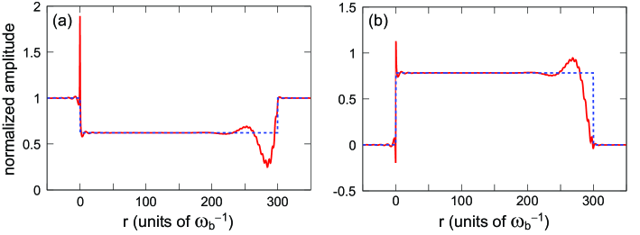
Figure 6: Normalized amplitude of the waveguide field, $\langle\widetilde{c}_{r}(t)\rangle/E(r,t)$. (a) Real and (b) imaginary parts. Solid lines represent the rigorous numerical results, and dotted lines represent the approximate one given by Eq. (42). The parameters are chosen as follows: $\kappa/\omega_{b}=0.1$, $k_{d}/\omega_{b}=0.6$, and $t=300/\omega_{b}$.

We switch to the real-space representation, $\langle\widetilde{c}_{r}(t)\rangle$, using Eq. (9). $\langle\widetilde{c}_{r}(t)\rangle^{(1)}$ is immediately given by

$$\langle\widetilde{c}_{r}(t)\rangle^{(1)} = E_{d}e^{ik_{d}(r-t)}.$$ (40)

Obviously, this is nothing but the input drive field of Eq. (7). Regarding $\langle\widetilde{c}_{r}(t)\rangle^{(2)}$, the principal contribution comes from the pole at $k=k_{d}+i0$ in the right-hand-side of Eq. (38). Therefore, we can employ the following approximation, $\langle c_{k}(t)\rangle_{s}^{(2)}\approx\sqrt{8\pi}\omega_{b}\xi_{k_{d}}^{2}E_{d}[k_{d}^{2}-\omega_{b}^{2}z^{*}(k_{d})]^{-1}[k-k_{d}-i0]^{-1}\left(e^{-ikt}-e^{-ik_{d}t}\right)$. Then, we have

$$\langle\widetilde{c}_{r}(t)\rangle^{(2)} \approx -\frac{4\pi i\omega_{b}\xi_{k_{d}}^{2}}{k_{d}^{2}-\omega_{b}^{2}z^{*}(k_{d})}\theta(r)\theta(t-r)E_{d}e^{ik_{d}(r-t)},$$ (41)

where $\theta$ is the Heaviside step function. This represents the radiation from the cavity emitted into the positive $r$ region. Finally, $\langle\widetilde{c}_{r}(t)\rangle^{(3)}$ yields no propagating wave. Combining these results, we obtain the following analytic form of $\langle\widetilde{c}_{r}(t)\rangle$:

$$\langle\widetilde{c}_{r}(t)\rangle \approx \left(1-\frac{4\pi i\omega_{b}\xi_{k_{d}}^{2}}{k_{d}^{2}-\omega_{b}^{2}z^{*}(k_{d})}\theta(r)\theta(t-r)\right)\times E_{d}e^{ik_{d}(r-t)}.$$ (42)

The spatial shape of $\langle\widetilde{c}_{r}(t)\rangle$ is plotted in Fig. 6, in which the rigorous shape [numerical Fourier transform of Eq. (36)] is plotted by solid lines and the approximate form [Eq. (42)] is plotted by dotted lines. We observe good agreement between them, except the deviations at the wavefront of the cavity radiation ($r\lesssim t$) and at the cavity position ($r\sim 0$). The former deviation originates in the transient cavity response, which is not taken into account in Eq. (42). The transient response vanishes within a timescale of $\kappa^{-1}$, which agrees with our observation in Fig. 6. On the other hand, the latter deviation around the cavity position originates in the fact that the cavity-waveguide interaction has a finite bandwidth in the wavenumber space and therefore is not spatially local in the present theoretical model. The bandwidth of the cavity-waveguide coupling is of the order of $\omega_{b}$ in the wavenumber space, and is therefore of the order of $\omega_{b}^{-1}$ in the real space. This explains the deviation localized at the origin in Fig. 6.

A notable fact is that, in contrast with the intracavity field amplitude [Eq. (27)] that is composed of both positively and negatively oscillating components, the waveguide field amplitude in the output port [Eq. (42)] is composed only of the positively oscillating one. Therefore, the elliptic motion is specific to the intracavity amplitude.

IV.4 Refection coefficient

The refection coefficient is identified as $R=\langle\widetilde{c}_{r}(t)\rangle/E(r,t)$ at the output port ($r>0$). From Eq. (42), $R$ is identified as

$$R(k_{d}) = 1-\frac{4\pi i\omega_{b}\xi_{k_{d}}^{2}}{k_{d}^{2}-\omega_{b}^{2}z^{*}(k_{d})}.$$ (43)

We can check that $|R|=1$ for any input frequency $k_{d}$. This implies that input field is reflected completely coherently, which is characteristic to linear optical response. In Fig. 7, we plot the phase shift upon reflection, $\arg R$, as a function of the drive frequency $k_{d}$, varying the cavity-waveguide coupling. As we increase the coupling, we observe the broadening of the linewidth and the redshift of the resonance frequency. The spectrum takes a kink-shaped form around the renormalized frequency. For a weak coupling, the spectrum is anti-symmetric with respect to the renormalized frequency, as is predicted by standard input-output theory. However, for a stronger coupling, such symmetry is gradually lost.

We can determine the renormalized resonance frequency $\widetilde{\omega}_{b}$ as the drive frequency achieving the $\pi$ phase shift, $R(\widetilde{\omega}_{b})=-1$. From this condition, $\widetilde{\omega}_{b}$ is analytically given by

$$\widetilde{\omega}_{b}^{2} = \frac{\omega_{b}^{2}-\omega_{x}^{2}+\sqrt{(\omega_{b}^{2}+\omega_{x}^{2})(\omega_{b}^{2}+\omega_{x}^{2}-4\kappa\omega_{x})}}{2}.$$ (44)

As we can confirm in Fig. 2, this is almost identical to the former definition of $\widetilde{\omega}_{b}$ by Eq. (5). We observe in Fig. 7 that the reflection coefficient becomes independent of the coupling strength $\kappa/\omega_{b}$ at the bare cavity resonance, $k_{d}=\omega_{b}$; we can check that $R(\omega_{b})=(\omega_{x}-i\omega_{b})/(\omega_{x}+i\omega_{b})$.

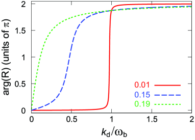
Figure 7: Phase shift upon reflection as a function of the drive frequency. The cavity-waveguide coupling strength, $\kappa/\omega_{b}$, is indicated.

IV.5 Open waveguide

In the previous subsection, we have determined the reflection coefficient $R$ when a semi-infinite waveguide is coupled to a cavity (Fig. 1). From this result, we can readily determine the reflection and transmission coefficients $R^{\prime}$ and $T^{\prime}$, when the cavity is coupled to an open waveguide [Fig. 8(a)]. The amplitude of waveguide field in this case is written as

$$E(r,t) = E_{d}e^{-i\omega_{d}t}\times\begin{cases}e^{ik_{d}r}+R^{\prime}e^{-ik_{d}r}&(r<0)\\ T^{\prime}e^{ik_{d}r}&(0<r)\end{cases}.$$ (45)

We divide this field into even and odd components. The even component interacts with the cavity whereas the odd component does not. The even component is defined by $E_{s}(r,t)=[E(r,t)+E(-r,t)]/2$ and is therefore given by $E_{s}(r,t)=\frac{1}{2}E_{d}e^{-ik_{d}(r+t)}+\frac{R^{\prime}+T^{\prime}}{2}E_{d}e^{ik_{d}(r-t)}$ for $r>0$. Since the first (second) term in the right-hand-side of this equation represents the incoming (outgoing) field, we have $R^{\prime}+T^{\prime}=R$. Similarly, the odd component is defined by $E_{a}(r,t)=[E(r,t)-E(-r,t)]/2$ and is therefore given by $E_{s}(r,t)=-\frac{1}{2}E_{d}e^{-ik_{d}(r+t)}+\frac{T^{\prime}-R^{\prime}}{2}E_{d}e^{ik_{d}(r-t)}$ for $r>0$. Since the incoming field simply transmits the cavity without interaction, we have $T^{\prime}-R^{\prime}=1$. Therefore,

$$R^{\prime} = (R-1)/2,$$ (46)

$$T^{\prime} = (R+1)/2.$$ (47)

We can readily confirm that $|R^{\prime}|^{2}+|T^{\prime}|^{2}=1$. The transmissivity $|T^{\prime}|^{2}$ is plotted in Fig. 8(b) as a function of the drive frequency. We observe that the symmetric transmission dip for a weak coupling case (solid line) gradually becomes asymmetric as the cavity-waveguide coupling increases (dashed and dotted lines).

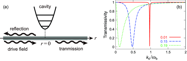
Figure 8: (a) Schematic of a cavity coupled to an open waveguide. (b) Transmissiveity $|T^{\prime}|^{2}$ as a function of the drive frequency. The cavity-waveguide coupling strength, $\kappa/\omega_{b}$, is indicated.

V summary

In this study, we investigated optical response of a linear waveguide QED system, namely, an optical cavity coupled to a waveguide. Our analysis is based on exact diagonalization of the overall Hamiltonian, and is therefore rigorous even in the ultrastrong and deep-strong coupling regimes of waveguide QED, in which the perturbative treatments of dissipation such as the Lindblad master equation are no longer valid. We observed that the motion of the cavity amplitude in the phase space is elliptical in general, owing to the counter-rotating terms in the cavity-waveguide coupling. Such elliptical motion becomes remarkable in the ultrastrong coupling regime due to the large Lamb shift of the cavity frequency comparable to its bare frequency. However, such an elliptical motion of the cavity amplitude is not reflected in the output field, contrary to the intuition by the input-output theory. We obtained an analytic expression of the reflection/transmission coefficient, which becomes asymmetric with respect to the resonance frequency as the cavity-waveguide coupling is increased.

Appendix A Fano diagonalization

From Eqs. (10) and (11), we have $[\hat{d}_{k},\hat{H}]=k\hat{d}_{k}$. This leads the following equations:

$$(k-\omega_{b})\beta_{1}(k) = \int_{0}^{\infty}dq\xi_{q}[\gamma_{1}(k,q)-\gamma_{2}(k,q)],$$ (48)

$$(k+\omega_{b})\beta_{2}(k) = \int_{0}^{\infty}dq\xi_{q}[\gamma_{1}(k,q)-\gamma_{2}(k,q)],$$ (49)

$$(k-q)\gamma_{1}(k,q) = \xi_{q}[\beta_{1}(k)-\beta_{2}(k)],$$ (50)

$$(k+q)\gamma_{2}(k,q) = \xi_{q}[\beta_{1}(k)-\beta_{2}(k)].$$ (51)

From Eqs. (49) and (51), we obtain $\beta_{2}(k)=\frac{k-\omega_{b}}{k+\omega_{b}}\beta_{1}(k)$ and $\gamma_{2}(k,q)=\frac{k-q}{k+q}\gamma_{1}(k,q)$. Then, Eqs. (48) and (50) are rewritten as

$$(k-\omega_{b})\beta_{1}(k) = 2\int_{0}^{\infty}dq\frac{q\xi_{q}}{k+q}\gamma_{1}(k,q),$$ (52)

$$(k-q)\gamma_{1}(k,q) = \frac{2\omega_{b}}{k+\omega_{b}}\beta_{1}(k)\xi_{q}.$$ (53)

Equation (53) is rewritten as

$$\gamma_{1}(k,q) = \frac{2\omega_{b}}{k+\omega_{b}}\beta_{1}(k)\xi_{q}\left(\frac{1}{k-q-i0}+y(k)\delta(k-q)\right),$$ (54)

where $y(k)$ is a quantity to be determined. Substituting the above equation into Eq. (52), and using $\int_{0}^{\infty}\frac{q\xi_{q}^{2}}{(k+q)(k-q-i0)}=\frac{1}{2}\int_{-\infty}^{\infty}\frac{\xi_{q}^{2}}{k-q-i0}$, $y(k)$ is given by

$$y(k) = \frac{1}{\xi_{k}^{2}}\left(\frac{k^{2}-\omega_{b}^{2}}{2\omega_{b}}-\Sigma(k)\right),$$ (55)

$$\Sigma(k) = \int_{-\infty}^{\infty}dq\frac{\xi_{q}^{2}}{k-q-i0}.$$ (56)

Note that $\Sigma(k)$ is the self-energy of the cavity, satisfying $\Sigma(-k)=\Sigma^{*}(k)$ and $\mathrm{Im}\Sigma(k)=\pi\xi_{k}^{2}$.

Up to here, we derived the expressions of $\beta_{2}$, $\gamma_{1}$ and $\gamma_{2}$ in terms of $\beta_{1}$. $\beta_{1}(k)$ is determined by the normalization condition, Eq. (11). This is rewritten as $\delta(k-k^{\prime})=\beta_{1}(k)\beta_{1}^{*}(k^{\prime})-\beta_{2}(k)\beta_{2}^{*}(k^{\prime})+\int_{0}^{\infty}dq[\gamma_{1}(k,q)\gamma_{1}^{*}(k^{\prime},q)-\gamma_{2}(k,q)\gamma_{2}^{*}(k^{\prime},q)]$, which leads to $\frac{2\omega_{b}\xi_{k}}{(k+\omega_{b})}|\beta_{1}(k)||y(k)|=1$. By adequately choosing the phase of $\beta_{1}$, we obtain Eq. (13),

$$\beta_{1}(k) = \frac{k+\omega_{b}}{2\omega_{b}\xi_{k}y(k)}=\frac{(k+\omega_{b})\xi_{k}}{k^{2}-\omega_{b}^{2}z(k)}.$$ (57)

$\beta_{2}$, $\gamma_{1}$ and $\gamma_{2}$ are obtained accordingly.

Appendix B transient component of cavity mode

Here we present the transient component of the cavity amplitude, $\langle\hat{b}(t)\rangle_{t}$, which is omitted in Sec. IV.1:

$$\langle\hat{b}(t)\rangle_{t} = \sqrt{8\pi}E_{d}\omega_{b}\xi_{k_{d}}\int_{-\infty}^{\infty}dq\frac{e^{-iqt}(q+\omega_{b})\xi_{q}^{2}}{(q-k_{d}-i0)[q^{2}-\omega_{b}^{2}z(q)][q^{2}-\omega_{b}^{2}z^{*}(q)]}$$ (58)

$$- \sqrt{8\pi}E_{d}^{*}\omega_{b}\xi_{k_{d}}\int_{-\infty}^{\infty}dq\frac{e^{iqt}(q-\omega_{b})\xi_{q}^{2}}{(q-k_{d}+i0)[q^{2}-\omega_{b}^{2}z(q)][q^{2}-\omega_{b}^{2}z^{*}(q)]}.$$

Using $\frac{\omega_{b}\xi_{q}^{2}}{[q^{2}-\omega_{b}^{2}z(q)][q^{2}-\omega_{b}^{2}z^{*}(q)]}=\frac{1}{4i\pi}(\frac{1}{q^{2}-\omega_{b}^{2}z(q)}-\frac{1}{q^{2}-\omega_{b}^{2}z^{*}(q)})$ and that $\frac{1}{q^{2}-\omega_{b}^{2}z(q)}$ has no poles on the lower half plane, transient component is rewritten as

$$\langle b(t)\rangle_{t} = \frac{iE_{d}\xi_{k_{d}}}{\sqrt{2\pi}}\int_{-\infty}^{\infty}dq\frac{e^{-iqt}(q+\omega_{b})}{(q-k_{d}-i0)[q^{2}-\omega_{b}^{2}z^{*}(q)]}+\frac{iE_{d}^{*}\xi_{k_{d}}}{\sqrt{2\pi}}\int_{-\infty}^{\infty}dq\frac{e^{iqt}(q-\omega_{b})}{(q-k_{d}+i0)[q^{2}-\omega_{b}^{2}z(q)]}.$$ (59)

Appendix C Integrals in Eqs. (32) and (33)

Here, we derive an analytical form of the integral in the right-hand-side of Eq. (32). From Eq. (18), we have $z(k)-z^{*}(k)=4i\pi\xi_{k}^{2}/\omega_{b}$. Therefore, the integral is rewritten as

$$\int_{0}^{\infty}dq|\beta_{2}(q)|^{2} = \frac{1}{4i\pi\omega_{b}}\left(\int_{0}^{\infty}dq\frac{(q-\omega_{b})^{2}}{q^{2}-\omega_{b}^{2}z(q)}-\mathrm{c.c.}\right).$$ (60)

We denote the integrand in the right-hand-side of Eq. (60) by $f(q)$. Using Eq. (22), $f(q)$ is rewritten as

$$f(q) = \frac{(q-\omega_{b})^{2}}{q^{2}-\omega_{b}^{2}z(q)}=\frac{(q-\omega_{b})^{2}(q-i\omega_{x})}{(q-\lambda_{1})(q-\lambda_{2})(q-\lambda_{3})}=1+\sum_{j=1}^{3}\frac{c_{j}}{q-\lambda_{j}},$$ (61)

where $c_{j}$ is a residue of $f(q)$ at $q=\lambda_{j}$. Substituting Eq. (61) into Eq. (60), we obtain

$$\int_{0}^{\infty}dq|\beta_{2}(q)|^{2} = -\frac{1}{2\pi\omega_{b}}\sum_{j=1}^{3}\mathrm{Im}\{c_{j}\log(-\lambda_{j})\}.$$ (62)

Repeating the same argument, the integral appearing in Eq. (33) is given by

$$-\int_{0}^{\infty}dq\beta_{1}^{*}(q)\beta_{2}(q) = -\frac{1}{2\pi\omega_{b}}\sum_{j=1}^{3}\mathrm{Im}\{d_{j}\log(-\lambda_{j})\},$$ (63)

where $d_{j}$ is a residue at $q=\lambda_{j}$ of the following function $g(q)$,

$$g(q) = \frac{(\omega_{b}^{2}-q^{2})(q-i\omega_{x})}{(q-\lambda_{1})(q-\lambda_{2})(q-\lambda_{3})}.$$ (64)

References

- (1) M. Brune, F. Schmidt-Kaler, A. Maali, J. Dreyer, E. Hagley, J. M. Raimond, and S. Haroche, Quantum Rabi Oscillation: A Direct Test of Field Quantization in a Cavity, Phys. Rev. Lett. 76, 1800 (1996).
- (2) J. McKeever, A. Boca, A. D. Boozer, J. R. Buck, and H. J. Kimble, Experimental realization of a one-atom laser in the regime of strong coupling, Nature 425, 268 (2003).
- (3) M. Keller, B. Lange, K. Hayasaka, W. Lange, and H. Walther, Deterministic coupling of single ions to an optical cavity, Appl. Phys. B 76, 125 (2003).
- (4) T. Yoshie, A. Scherer, J. Hendrickson, G. Khitrova, H. M. Gibbs, G. Rupper, C. Ell, O. B. Shchekin, and D. G. Deppe, Vacuum Rabi splitting with a single quantum dot in a photonic crystal nanocavity, Nature 432, 200 (2004).
- (5) G. Gunter, A. A. Anappara, J. Hees, A. Sell, G. Biasiol, L. Sorba, S. D. Liberato, C. Ciuti, A. Tredicucci, A. Leitenstorfer, and R. Huber, Sub-cycle switch-on of ultrastrong light-matter interaction, Nature 458, 178, (2009).
- (6) T. Niemczyk, F. Deppe, H. Huebl, E. P. Menzel, F. Hocke, M. J. Schwarz, J. J. Garcia-Ripoll, D. Zueco, T. Hummer, E. Solano, A. Marx, and R. Gross, Circuit quantum electrodynamics in the ultrastrong-coupling regime, Nat. Phys. 6, 772 (2010).
- (7) S. Gambino, M. Mazzeo, A. Genco, O. D. Stefano, S. Savasta, S. Patane, D. Ballarini, F. Mangione, G. Lerario, D. Sanvitto, and G. Gigli, Exploring light-matter interaction phenomena under ultrastrong coupling regime, ACS Photon. 1, 1042 (2014).
- (8) A. Bayer, M. Pozimski, S. Schambeck, D. Schuh, R. Huber, D. Bougeard, and C. Lange, Terahertz light-matter interaction beyond unity coupling strength, Nano Lett. 17, 6340 (2017).
- (9) X. Li, M. Bamba, Q. Zhang, S. Fallahi, G. C. Gardner, W. Gao, M. Lou, K. Yoshioka, M. J. Manfra, and J. Kono, Vacuum Bloch-Siegert shift in Landau polaritons with ultra-high cooperativity, Nat. Photon. 12, 324 (2018).
- (10) F. Yoshihara, T. Fuse, S. Ashhab, K. Kakuyanagi, S. Saito, and K. Semba, Superconducting qubit-oscillator circuit beyond the ultrastrong-coupling regime, Nat. Phys. 13, 44 (2017).
- (11) F. Yoshihara, T. Fuse, Z. Ao, S. Ashhab, K. Kakuyanagi, S. Saito, T. Aoki, K. Koshino, and K. Semba, Inversion of qubit energy levels in qubit-oscillator circuits in the deep-strong-coupling regime, Phys. Rev. Lett. 120, 183601 (2018).
- (12) P. Forn-Diaz, J. Lisenfeld, D. Marcos, J. J. Garcia-Ripoll, E. Solano, C. J. P. M. Harmans, and J. E. Mooij, Observation of the Bloch-Siegert Shift in a Qubit-Oscillator System in the Ultrastrong Coupling Regime, Phys. Rev. Lett. 105, 237001 (2010).
- (13) S.-P. Wang, G.-Q. Zhang, Y. Wang, Z. Chen, T. Li, J. S. Tsai, S.-Y. Zhu, J. Q. You, Photon-Dressed Bloch-Siegert Shift in an Ultrastrongly Coupled Circuit Quantum Electrodynamical System, Phys. Rev. Appl. 13, 054063 (2020).
- (14) C. Ciuti, G. Bastard and I. Carusotto, Quantum vacuum properties of the intersubband cavity polariton field, Phys. Rev. B 72, 115303 (2005).
- (15) V. V. Dodonov and A. V. Dodonov, QED effects in a cavity with a time-dependent thin semiconductor slab excited by laser pulses, J. Phys. B 39, 1 (2006).
- (16) A. Auer and G. Burkard, Entangled photons from the polariton vacuum in a switchable optical cavity, Phys. Rev. B 85, 235140 (2012).
- (17) M. Cirio, S. De Liberato, N. Lambert, and F. Nori, Ground State Electroluminescence, Phys. Rev. Lett. 116, 113601 (2016).
- (18) S. De Liberato, Virtual photons in the ground state of a dissipative system, Nat. Commun. 8, 1 (2017).
- (19) C. K. Law, Vacuum Rabi oscillation induced by virtual photons in the ultrastrong-coupling regime, Phys. Rev. A 87, 045804 (2013).
- (20) L. Garziano, R. Stassi, V. Macri, A. F. Kockum, S. Savasta, and F. Nori, Multiphoton quantum Rabi oscillations in ultrastrong cavity QED, Phys. Rev. A 92, 063830 (2015).
- (21) A. F. Kockum, A. Miranowicz, V. Macri, S. Savasta, and F. Nori, Deterministic quantum nonlinear optics with single atoms and virtual photons, Phys. Rev. A 95, 063849 (2017).
- (22) O. Astafiev, A. M. Zagoskin, A. A. Abdumalikov Jr., Yu. A. Pashkin, T. Yamamoto, K. Inomata, Y. Nakamura, and J. S. Tsai, Resonance fluorescence of a single artificial atom, Science 327, 840 (2010).
- (23) I.-C. Hoi, A. F. Kockum, T. Palomaki, T. M. Stace, B. Fan, L. Tornberg, S. R. Sathyamoorthy, G. Johansson, P. Delsing, and C. M. Wilson, Giant cross-Kerr effect for propagating microwaves induced by an artificial atom, Phys. Rev. Lett. 111, 053601 (2013).
- (24) A. F. van Loo, A. Fedorov, K. Lalumiere, B. C. Sanders, A. Blais, and A. Wallraff, Photon-mediated interactions between distant artificial atoms, Science 342, 1494 (2013).
- (25) K. Koshino, H. Terai, K. Inomata, T. Yamamoto, W. Qiu, Z. Wang, and Y. Nakamura, Observation of three-state dressed states in circuit quantum electrodynamics, Phys. Rev. Lett. 110, 263601 (2013).
- (26) A. Goban, C.-L. Hung, J. D. Hood, S.-P. Yu, J. A. Muniz, O. Painter, and H. J. Kimble, Superradiance for atoms trapped along a photonic crystal waveguide, Phys. Rev. Lett. 115, 063601 (2015).
- (27) M. Arcari, I. Sollner, A. Javadi, S. Lindskov Hansen, S. Mahmoodian, J. Liu, H. Thyrrestrup, E. H. Lee, J. D. Song, S. Stobbe, and P. Lodahl, Near-unity coupling efficiency of a quantum emitter to a photonic crystal waveguide, Phys. Rev. Lett. 113, 093603 (2014).
- (28) P. Forn-Diaz, J. J. Garcia-Ripoll, B. Peropadre, J. L. Orgiazzi, M. A. Yurtalan, R. Belyansky, C. M. Wilson, and A. Lupascu, Ultrastrong coupling of a single artificial atom to an electromagnetic continuum in the nonperturbative regime, Nat. Phys. 13, 39 (2017).
- (29) J. Puertas Martinez, S. Leger, N. Gheeraert, et al., A tunable Josephson platform to explore many-body quantum optics in circuit-QED npj Quantum Inf 5, 19 (2019).
- (30) D. F. Walls and G. J. Milburn, Quantum Optics, (Springer, Berlin, 1995).
- (31) D. Manzano, A short introduction to the Lindblad Master Equation, arXiv:1906.04478 (2019).
- (32) B. Peropadre, D. Zueco, D. Porras, and J. J. Garcia-Ripoll, Nonequilibrium and Nonperturbative Dynamics of Ultrastrong Coupling in Open Lines, Phys. Rev. Lett. 111, 243602 (2013).
- (33) G. Diaz-Camacho, A. Bermudez, and J. J. Garcia-Ripoll, Dynamical polaron Ansatz: A theoretical tool for the ultrastrong-coupling regime of circuit QED, Phys. Rev. A 93, 043843 (2016).
- (34) D. Zueco and J. Garcia-Ripoll, Ultrastrongly dissipative quantum Rabi model, Phys. Rev. A 99, 013807 (2019).
- (35) W. S. Teixeira, F. L. Semiao, J. Tuorila, and M. Mottonen, Numerically exact treatment of dissipation in a driven two-level system, arXiv:2011.06106 (2020).
- (36) U. Fano, Effects of Configuration Interaction on Intensities and Phase Shifts, Phys. Rev., 124 1866 (1961).
- (37) B. Huttner and S. M. Barnett, Quantization of the electromagnetic field in dielectrics, Phys. Rev. A 46, 4306 (1992).
- (38) M. R. da Costa, A. O. Caldeira, S. M. Dutra, and H. Westfahl Jr., Exact diagonalization of two quantum models for the damped harmonic oscillator, Phys. Rev. A 61, 022107 (2000).
- (39) The mode function is normalized so as to satisfy .