Average-Reward Off-Policy Policy Evaluation with Function Approximation

Abstract

We consider off-policy policy evaluation with function approximation (FA) in average-reward MDPs, where the goal is to estimate both the reward rate and the differential value function. For this problem, bootstrapping is necessary and, along with off-policy learning and FA, results in the deadly triad (Sutton & Barto, 2018). To address the deadly triad, we propose two novel algorithms, reproducing the celebrated success of Gradient TD algorithms in the average-reward setting. In terms of estimating the differential value function, the algorithms are the first convergent off-policy linear function approximation algorithms. In terms of estimating the reward rate, the algorithms are the first convergent off-policy linear function approximation algorithms that do not require estimating the density ratio. We demonstrate empirically the advantage of the proposed algorithms, as well as their nonlinear variants, over a competitive density-ratio-based approach, in a simple domain as well as challenging robot simulation tasks.

shangtong

1 Introduction

A fundamental problem in average-reward Markov Decision Processes (MDPs, see, e.g., Puterman (1994)) is policy evaluation, that is, estimating, for a given policy, the reward rate and the differential value function. The reward rate of a policy is the average reward per step and thus measures the policy’s long term performance. The differential value function summarizes the expected cumulative future excess rewards, which are the differences between received rewards and the reward rate. The solution of the policy evaluation problem is interesting in itself because it provides a useful performance metric, the reward rate, for a given policy. In addition, it is an essential part of many control algorithms, which aim to generate a policy that maximizes the reward rate by iteratively improving the policy using its estimated differential value function (see, e.g., Howard (1960); Konda (2002); Abbasi-Yadkori et al. (2019)).

One typical approach in policy evaluation is to learn from real experience directly, without knowing or learning a model. If the policy followed to generate experience (behavior policy) is the same as the policy of interest (target policy), then this approach yields an on-policy method; otherwise, it is off-policy. Off-policy methods are usually more practical in settings in which following bad policies incurs prohibitively high cost (Dulac-Arnold et al., 2019). For policy evaluation, we can use either tabular methods, which maintain a look-up table to store quantities of interest (e.g., the differential values for all states) separately, or use function approximation, which represents these quantities collectively, possibly in a more efficient way (e.g., using a neural network). Function approximation methods are necessary for MDPs with large state and/or action spaces because they are scalable in the size of these spaces and also generalize to states and actions that are not in the data (Mnih et al., 2015; Silver et al., 2016). Finally, for the policy evaluation problem in average reward MDPs, the agent’s stream of experience never terminates and thus actual returns cannot be obtained. Because of this, learning algorithms have to bootstrap, that is, the estimated values must be updated towards targets that include existing estimated values instead of actual returns.

In this paper, we consider methods for solving the average-reward policy evaluation problem with all the above three elements (off-policy learning, function approximation and bootstrapping), which comprise the deadly triad (see Chapter 11 of Sutton & Barto (2018) and Section 3). The main contributions of this paper are two newly proposed methods to break this deadly triad in the average-reward setting, both of which are inspired by the celebrated success of the Gradient TD family of algorithms (Sutton et al., 2009b, a) in breaking the deadly triad in the discounted setting.

Few methods exist for learning differential value functions. These are either on-policy linear function approximation methods (Tsitsiklis & Van Roy, 1999; Konda, 2002; Yu & Bertsekas, 2009; Abbasi-Yadkori et al., 2019) or off-policy tabular methods (Wan et al., 2020). The on-policy methods use the empirical average of received rewards as an estimate for the reward rate. Thus they are not straightforward to extend to the off-policy case. And, as we show later with a counterexample, the naive extension of the off-policy tabular method by Wan et al. (2020) to the linear function approximation setting can diverge, exemplifying the deadly triad. By contrast, the two algorithms we propose are the first provably convergent methods for learning the differential value function via off-policy linear function approximation.

All existing methods for estimating reward rate in off-policy function approximation setting require learning the density ratio, i.e., the ratio between the stationary distribution of the target policy and the sampling distribution (Liu et al., 2018a; Zhang et al., 2020a, b; Mousavi et al., 2020; Lazic et al., 2020). Interestingly, while density-ratio-based methods dominate off-policy policy evaluation with function approximation in average-reward MDPs, in the discounted MDPs, both density-ratio-based (Hallak & Mannor, 2017; Liu et al., 2018a; Gelada & Bellemare, 2019; Nachum et al., 2019a; Uehara & Jiang, 2019; Xie et al., 2019; Tang et al., 2019; Zhang et al., 2020a, b) and value-based (Baird, 1995; Sutton et al., 2009b, a, 2016; Thomas et al., 2015; Jiang & Li, 2015) methods have succeeded. It thus remains unknown whether a convergent value-based method could be found for such a problem and if it exists, how it performs compared with density-ratio-based methods. The two algorithms we propose are the first provably convergent differential-value-based methods for reward rate estimation via off-policy linear function approximation, which answer the question affirmatively. Furthermore, our empirical study shows that our value-based methods consistently outperform a competitive density-ratio-based approach, GradientDICE (Zhang et al., 2020b), in the tested domains, including both a simple Markov chain and challenging robot simulation tasks.

2 Background

In this paper, we use $\norm{\cdot}_{M}$ to denote the vector norm induced by a positive definite matrix $M$, i.e., $\norm{x}_{M}=\sqrt{x^{\top}Mx}$. We also use $\norm{\cdot}_{M}$ to denote the corresponding induced matrix norm. When $M=I$, we ignore the subscript $I$ and write $\norm{\cdot}$ for simplicity. All vectors are column vectors. 0 denotes an all-zero vector whose dimension can be deduced from the context. 1 is similarly defined. When it does not confuse, we use a function and a vector interchangeably. For example, if $f$ is a function from $\mathcal{X}$ to $\mathbb{R}$, we also use $f$ to denote the corresponding vector in $\mathbb{R}^{|\mathcal{X}|}$.

We consider an infinite horizon MDP with a finite state space $\mathcal{S}$, a finite action space $\mathcal{A}$, a reward function $r:\mathcal{S}\times\mathcal{A}\to\mathbb{R}$, and a transition kernel $p:\mathcal{S}\times\mathcal{S}\times\mathcal{A}\to[0,1]$. When an agent follows a policy $\pi:\mathcal{A}\times\mathcal{S}\to[0,1]$ in the MDP, at time step $t$, the agent observes a state $S_{t}$, takes an action $A_{t}\sim\pi(\cdot|S_{t})$, receives a reward $r(S_{t},A_{t})$, proceeds to the next time step and observes the next state $S_{t+1}\sim p(\cdot|S_{t},A_{t})$. The reward rate of policy $\pi$ is defined as

$$\textstyle{r_{\pi}\doteq C\text{-}\lim_{t\to\infty}\mathbb{E}[r(S_{t},A_{t})\mid\pi,S_{0}]},$$ (1)

where $C\text{-}\!\lim_{T\to\infty}z_{T}\doteq\lim_{T\to\infty}\frac{1}{T+1}\sum_{i=0}^{T}z_{i}$ is the Cesaro limit. The Cesaro limit in (1) is assumed to exist and is independent of $S_{0}$. The most general assumption that guarantees these is the following one:

Assumption 2.1.

Policy $\pi$ induces a unichain.

The action-value function in the average-reward setting is known as the differential action-value function and is defined as $q_{\pi}(s,a)\doteq\textstyle{C\text{-}\lim_{T\to\infty}}\textstyle{\sum_{t=0}^{T}\mathbb{E}[r(S_{t},A_{t})-r_{\pi}\mid S_{0}=s,A_{0}=a]}$. Note that if a stronger ergodic chain assumption is used instead, the Cesaro limit in defining $r_{\pi}$ and $q_{\pi}$ is equivalent to the normal limit. The action-value Bellman equation is

$$q=r-\bar{r}{\textbf{1}}+P_{\pi}q,$$ (2)

where $q\in\mathbb{R}^{|\mathcal{S}||\mathcal{A}|}$ and $\bar{r}\in\mathbb{R}$ are free variables and $P_{\pi}\in\mathbb{R}^{{|\mathcal{S}||\mathcal{A}|}\times{|\mathcal{S}||\mathcal{A}|}}$ is the transition matrix, that is, $P_{\pi}((s,a),(s^{\prime},a^{\prime}))\doteq p(s^{\prime}|s,a)\pi(a^{\prime}|s^{\prime})$. It is well-known (Puterman, 1994) that $r=r_{\pi}$ is the unique solution for $r$ and all the solutions for $q$ form a set $\{q_{\pi}+c{\textbf{1}}:\forall c\in\mathbb{R}\}$.

In this paper, we consider a special off-policy learning setting, where the agent learns from i.i.d. samples drawn from a given sampling distribution. In particular, at the $k$-th iteration, the agent draws a sample $(S_{k},A_{k},R_{k},S_{k}^{\prime},A_{k}^{\prime})$ from a given sampling distribution $d_{\mu\pi}$. Distribution $d_{\mu\pi}$ can be any distribution satisfying

Assumption 2.2.

$R_{k}=r(S_{k},A_{k})$, $S_{k}^{\prime}\sim p(\cdot|S_{k},A_{k})$, $A_{k}^{\prime}\sim\pi(\cdot|S_{k}^{\prime})$, and $d_{\mu}(s,a)>0$ for all $(s,a)$,

where $d_{\mu}(s,a)$ denotes the marginal distribution of $(S_{k},A_{k})$. The last part of Assumption 2.2 means that every state-action pair is possible to be sampled. This is a necessary condition for learning the differential value function accurately for all state-action pairs. In the rest of the paper, the expectation $\mathbb{E}$ is taken w.r.t. $d_{\mu\pi}$.

If no sampling distribution is given, one could instead draw samples in the following way. First randomly sample $(S_{k},A_{k},R_{k},S_{k}^{\prime})$ from a batch of transitions collected by one or multiple agents, with all agents following possibly different unknown policies in the same MDP. Then sample $A_{k}^{\prime}\sim\pi(\cdot\mid S_{k}^{\prime})$. Assuming that the number of all state-action pairs in the batch grows to infinity as the batch size grows to infinity then sampling from the batch is approximately equivalent to sampling from some distribution satisfying Assumption 2.2.

Our goal is to approximate, using the data generated from $d_{\mu\pi}$, both the reward rate and the differential value function. The reward rate $r_{\pi}$ is approximated by a learnable scalar $\hat{r}$. The differential value function $q_{\pi}$ is only approximated up to a constant. That is, we are only interested in approximating $q_{\pi}+c{\textbf{1}}$ for some $c\in R$. This is sufficient if the approximated value function is only used for policy improvement in a control algorithm. However, when the state and/or action spaces are large, function approximation may be necessary to represent $q_{\pi}+c{\textbf{1}}$. This paper mainly considers linear function approximation, where the agent is given a feature mapping $x$ that generates a $K$-dimensional vector $x(s,a)$ given a state-action pair $(s,a)$. The agent further maintains a learnable weight vector $w\in\mathbb{R}^{K}$ and adjusts it to approximate, for all $(s,a)$, $q_{\pi}(s,a)+c$ using $x(s,a)^{\top}w$. Let $X\in\mathbb{R}^{{|\mathcal{S}||\mathcal{A}|}\times K}$ be the feature matrix whose $(s,a)$ row is $x(s,a)^{\top}$. For the uniqueness of the solution for $w$, it is common to make the following assumption:

Assumption 2.3.

$X$ has linearly independent columns.

3 Differential Semi-Gradient $Q$ Evaluation

We first present Differential Semi-gradient $Q$ Evaluation (Diff-SGQ), which is a straightforward extension of the tabular off-policy Differential TD-learning algorithm (Wan et al., 2020) to linear function approximation.

At the $k$-th iteration, the algorithm draws a sample $(S_{k},A_{k},R_{k},S_{k}^{\prime},A_{k}^{\prime})$ from $d_{\mu\pi}$ and updates $w_{k}$ and $\hat{r}_{k}$ as

$$w_{k+1} \doteq w_{k}+\alpha_{k}\delta_{k}(w_{k},\hat{r}_{k})x_{k},$$ (3)

$$\hat{r}_{k+1} \doteq\hat{r}_{k}+\alpha_{k}\delta_{k}(w_{k},\hat{r}_{k}),$$ (4)

where $\alpha_{k}$ is the stepsize used at $k$-th iteration, $x_{k}\doteq x(S_{k},A_{k})$, $x_{k}^{\prime}\doteq x(S_{k}^{\prime},A_{k}^{\prime})$, and $\delta_{k}(w,\hat{r})\doteq R_{k}-\hat{r}+x_{k}^{\prime\top}w-x_{k}^{\top}w$ is the temporal difference error. From (2), it is easy to see $r_{\pi}=d^{\top}(r+P_{\pi}q_{\pi}-q_{\pi})$ holds for any probability distribution $d$; in particular, it holds for $d=d_{\mu}$, which is the intuition behind the $\hat{r}$ update (4).Diff-SGQ iteratively solves

$$\mathbb{E}[\delta_{k}(w,\hat{r})x_{k}]={\textbf{0}},\mbox{\quad and\quad}\mathbb{E}[\delta_{k}(w,\hat{r})]=0,$$ (5)

whose solutions, if they exist, are TD fixed points. A TD fixed point is an approximate solution to (2) using linear function approximation. We consider the quality of the approximation in the next section. All the proposed algorithms in this paper aim to find a TD fixed point up to some regularization bias if necessary.

In general, there could be no TD fixed point, one TD fixed point, or infinitely many TD fixed points, as in the discounted setting. To see this, let $y_{k}\doteq[1,x^{\top}_{k}]^{\top}$, $y_{k}^{\prime}\doteq[1,x^{\prime\top}_{k}]^{\top},u\doteq[\hat{r},w^{\top}]^{\top}$, and $e_{1}\doteq[1,0,\cdots,0]^{\top}\in\mathbb{R}^{K+1}$. Then combining (3) and (4) gives

$$\mathbb{E}[\delta_{k}(u)y_{k}]={\textbf{0}},$$ (6)

where $\delta_{k}(u)\doteq R_{k}-e_{1}^{\top}u+y_{k}^{\prime\top}u-y_{k}^{\top}u$. Writing (6) in vector form, we have $Au+b={\textbf{0}}$, where

(7)

(8)

(9)

If and only if $A$ is invertible, there exists a unique TD fixed point

$$u_{\text{TD}}\doteq-A^{-1}b.$$ (10)

Otherwise, there is either no TD fixed point or there are infinitely many.

Unfortunately, even if there exists a unique TD fixed point, Diff-SGQ can still diverge, which exemplifies the deadly triad (Sutton & Barto, 2018) in the average-reward setting. The following example confirms this point.

Example 1 (The divergence of Diff-SGQ).

Consider a two-state MDP (Figure 1). The expected Diff-SGQ update per step can be written as $\matrixquantity[\hat{r}_{k+1}\\ w_{k+1}]=\matrixquantity[\hat{r}_{k}\\ w_{k}]+\alpha\left(A\matrixquantity[\hat{r}_{k}\\ w_{k}]+b\right)=\matrixquantity[\hat{r}_{k}\\ w_{k}]+\alpha\matrixquantity[-1&6\\ -2&6]\matrixquantity[\hat{r}_{k}\\ w_{k}].$ Here, we consider $\alpha$ a constant stepsize. The eigenvalues of $A=\matrixquantity[-1&6\\ -2&6]$ are both positive. Hence, no matter what positive stepsize is picked, the expected update diverges. The sample updates (3) and (4) using standard stochastic approximation stepsizes, therefore, also diverge. Furthermore, because both eigenvalues are positive, A is an invertible matrix, implying the unique existence of the TD fixed-point.

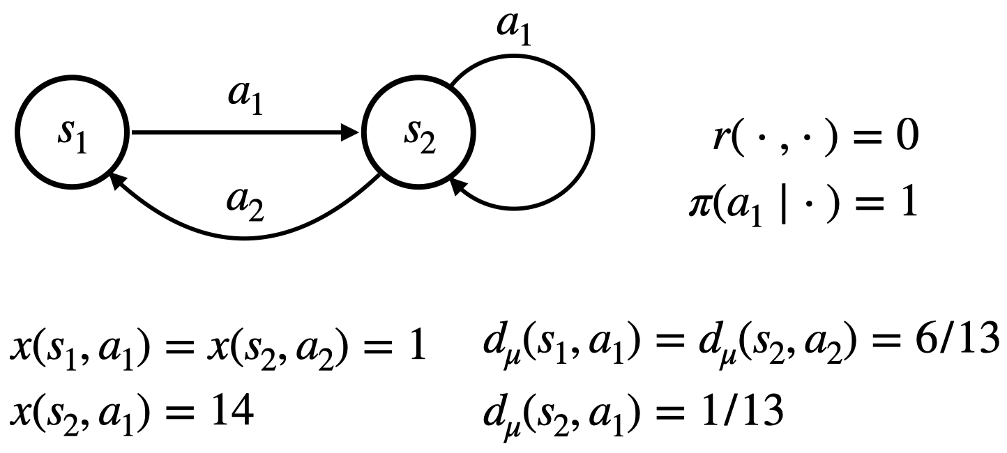
Figure 1: An example showing the divergence of Diff-SGQ.

4 One-Stage Differential Gradient $Q$ Evaluation

We now present an algorithm that is guaranteed to converge to the TD fixed point $\eqref{eq: TD fixed point variant}$ if it uniquely exists. Motivated by the Mean Squared Projected Bellman Error (MSPBE) defined in the discounted setting and used by Gradient TD algorithms, we define the MSPBE in the average-reward setting as

$$\text{MSPBE}_{1}(u) =\norm{\Pi_{Y}\bar{\delta}(u)}^{2}_{D},$$ (11)

where $\Pi_{Y}\doteq Y(Y^{\top}DY)^{-1}Y^{\top}D$ is the projection matrix and $\bar{\delta}(u)\doteq r-e_{1}^{\top}u{\textbf{1}}+P_{\pi}Yu-Yu$ is the vector of TD errors for all state-action pairs. The vector $\Pi_{Y}\bar{\delta}(u)$ is the projection of the vector of TD errors on the column space of $Y$. The existence of the matrix inverse in $\Pi_{Y}$, $(Y^{\top}DY)^{-1}$, is guaranteed by Assumption 2.2 and

Assumption 4.1.

For any $w\in\mathbb{R}^{K}$ such that $w\neq{\textbf{0}}$ and for any $c\in\mathbb{R}$, $Xw\neq c{\textbf{1}}$.

The above assumption guarantees that if $w^{*}$ is a solution for $w$ in (5), then no other solution’s approximated action-value function would be identical to $Xw^{*}$ up to a constant. This assumption is also used by Tsitsiklis & Van Roy (1999) in their on-policy policy evaluation algorithms in average-reward MDPs. Apparently the assumption does not hold in the tabular setting (i.e., when $X=I$). However, with function approximation, we usually have many more states than features (i.e., ${|\mathcal{S}|}\gg K$), in which case the above assumption would not be restrictive.

Let $C\doteq Y^{\top}DY$, we have $\Pi^{\top}D\Pi=DYC^{-1}Y^{\top}D$, with which we give a different form for (11):

$$\text{MSPBE}_{1}(u) =\norm{Y^{\top}D\bar{\delta}(u)}^{2}_{C^{-1}}=\norm{Au+b}^{2}_{C^{-1}}$$ (12)

$$=\mathbb{E}[\delta_{k}(u)y_{k}]^{\top}\mathbb{E}[y_{k}y_{k}^{\top}]^{-1}\mathbb{E}[\delta_{k}(u)y_{k}].$$ (13)

It can be seen that if (6) has a solution, then that solution also minimizes (12), in which case solving (6) can be converted to minimizing (12). However, when (6) does not have a unique solution, the set of minimizers of (12) could be unbounded and thus algorithms minimizing $\text{MSPBE}_{1}$ risk generating unbounded updates. To ensure the stability of our algorithm when (6) does not have a unique solution, we use a regularized $\text{MSPBE}_{1}$ as our objective:

$$J_{1,\eta}(u)\doteq\norm{Au+b}_{C^{-1}}^{2}+\eta u^{\top}I_{0}u,$$ (14)

where $I_{0}\doteq diag({\textbf{1}}-e_{1})$, $\eta$ is a positive scalar, and $\eta u^{\top}I_{0}u=\eta\norm{w}^{2}$ is a ridge regularization term on $w$.

To minimize $J_{1,\eta}(u)$, one could proceed with techniques used in TDC (Sutton et al., 2009a), which we leave for future work. In this paper, we proceed with the saddle-point formulation of GTD2 introduced by Liu et al. (2015), which exploits Fenchel’s duality:

$$u^{\top}M^{-1}u=\max_{\nu}2u^{\top}\nu-\nu^{\top}M\nu,$$ (15)

for any positive definite $M$, yielding

$$J_{1,\eta}(u)$$ (16)

$$= \textstyle{\max_{\nu\in\mathbb{R}^{K+1}}2\nu^{\top}Y^{\top}D\bar{\delta}(u)-\nu^{\top}C\nu+\eta u^{\top}I_{0}u}.$$ (17)

So $\min_{u}J_{1,\eta}(u)=\min_{u}\max_{\nu}J_{1,\eta}(u,\nu)$, where

$$J_{1,\eta}(u,\nu)\doteq 2\nu^{\top}Y^{\top}D\bar{\delta}(u)-\nu^{\top}C\nu+\eta u^{\top}I_{0}u.$$ (18)

As $J_{1,\eta}(u,\nu)$ is convex in $u$ and concave in $\nu$, we have now reduced the problem into a convex-concave saddle point problem. Applying primal-dual methods to this problem, that is, performing gradient ascent for $\nu$ following $\nabla_{\nu}J_{1,\eta}(u,\nu)$ and gradient descent for $u$ following $\nabla_{u}J_{1,\eta}(u,\nu)$, we arrive at our first new algorithm, One-Stage Differential Gradient $Q$ Evaluation, or Diff-GQ1. At the $k$-th iteration, with a sample $(S_{k},A_{k},R_{k},S_{k}^{\prime},A_{k}^{\prime})$ from $d_{\mu\pi}$, Diff-GQ1 updates $u_{k}$ and $\nu_{k}$ as

$$\delta_{k} \doteq R_{k}-e_{1}^{\top}u_{k}+y_{k}^{\prime\top}u_{k}-y_{k}^{\top}u_{k},$$ (19)

$$\nu_{k+1} \doteq\nu_{k}+\alpha_{k}(\delta_{k}-y_{k}^{\top}\nu_{k})y_{k},$$ (20)

$$u_{k+1} \doteq u_{k}+\alpha_{k}(y_{k}-y_{k}^{\prime}+e_{1})y_{k}^{\top}\nu_{k}-\alpha_{k}\eta I_{0}u_{k},$$ (21)

where $\quantity{\alpha_{k}}$ is the sequence of learning rates satisfying the following standard assumption:

Assumption 4.2.

$\{\alpha_{k}\}$ is a positive deterministic nonincreasing sequence s.t. $\sum_{k}\alpha_{k}=\infty$ and $\sum_{k}\alpha_{k}^{2}<\infty$.

The algorithm is one-stage because, while there are two weight vectors updated in every iteration, both converge simultaneously.

Theorem 1.

If Assumptions 2.1, 2.2, 4.1, & 4.2 hold, then for any $\eta>0$, almost surely, the iterate $\quantity{u_{k}}$ generated by Diff-GQ1 (19) converges to $u_{\eta}^{*}$, where $u^{*}_{\eta}\doteq-(\eta I_{0}+A^{\top}C^{-1}A)^{-1}A^{\top}C^{-1}b$ is the unique minimizer of $J_{1,\eta}(u)$. Further, if $A$ is invertible, then for $\eta=0$, $\quantity{u_{k}}$ converges almost surely to the $u_{\text{TD}}$ defined in (10).

We defer the full proof to Section A.1.

Proof.

(Sketch) With $\kappa_{k}\doteq[\nu_{k}^{\top},u_{k}^{\top}]^{\top}$, we rewrite (19) as

$$\kappa_{k+1}\doteq\kappa_{k}+\alpha_{k}(G_{k+1}\kappa_{k}+h_{k+1}),$$ (22)

where

(23)

The asymptotic behavior of $\quantity{\kappa_{k}}$ is governed by

The convergence of $\kappa_{t}$ to a unique point can be guaranteed if $\bar{G}$ is a Hurwitz matrix, or equivalently, if the real part of any eigenvalue of $\bar{G}$ is strictly negative. Therefore, it is important to first ensure that $\bar{G}$ is nonsingular. If $A$ was nonsingular, we can show $\bar{G}$ being nonsingular easily even with $\eta=0$. However, in general, $A$ may not be nonsingular and therefore, we require $\eta>0$ to ensure $\bar{G}$ being nonsingular. We can easily show that the real part of any eigenvalue of $\bar{G}$ is strictly negative and thus $\bar{G}$ is Hurwitz. Standard stochastic approximation results (Borkar, 2009) then show $\textstyle{\lim_{k}\kappa_{k}=-\bar{G}^{-1}\bar{h}}.$ Define $u^{*}_{\eta}$ as the lower half of $-\bar{G}^{-1}\bar{h}$, we have $u^{*}_{\eta}=-(\eta I_{0}+A^{\top}C^{-1}A)^{-1}A^{\top}C^{-1}b.$ It is easy to verify (e.g., using the first order optimality condition of $J_{1,\eta}(u)$) that $u^{*}_{\eta}$ is the unique minimizer of $J_{1,\eta}(u)$. ∎

Quality of TD Fixed Points. We now analyze the quality of TD fixed points. For our analysis, we make the following assumption.

Assumption 4.3.

There exists at least one TD fixed point.

Let $u^{*}=[\hat{r}^{*},w^{*\top}]^{\top}$ be one fixed point (a solution of (6)). We are interested in the upper bound of the absolute value of the difference between the estimated reward rate and the true reward rate $|\hat{r}^{*}-r_{\pi}|$ and also the upper bound of the minimum distance between the estimated differential value function to the set $\quantity{q_{\pi}+c{\textbf{1}}}$. In general, as long as there is representation error, the TD fixed point can be arbitrarily poor in terms of approximating the value function, even in the discounted case (see Kolter (2011) for more discussion). In light of this, we study the bounds only when $d_{\mu}$ is close to $d_{\pi}$, the stationary state-action distribution of $\pi$, in the sense of the following assumption. Let $\xi\in(0,1)$ be a constant,

Assumption 4.4.

$F$ is positive semidefinite, where

$$F\doteq\matrixquantity[X^{\top}DX$&X^{\top}DP_{\pi}X\\ X^{\top}P_{\pi}^{\top}DX&\xi^{2}X^{\top}DX]$$

A similar assumption about $F$ is also used by Kolter (2011) in the analysis of the performance of the MSPBE minimizer in the discounted setting. Kolter (2011) uses $\xi=1$ while we use $\xi<1$ to account for the lack of discounting. In Section D.1, we show with simulation that this assumption holds with reasonable probability in our randomly generated MDPs. Furthermore, we consider the bounds when all the features have zero mean under the distribution $d_{\mu}$.

Assumption 4.5.

$X^{\top}d_{\mu}={\textbf{0}}$.

This can easily be done by subtracting each feature vector sampled in our learning algorithm by some estimated mean feature vector, which is the empirical average of all the feature vectors sampled from $d_{\mu}$. Note without this mean-centered feature assumption, a looser bound can also be obtained. Our intention here is to show that bounds of our algorithms are on par with their counterparts in the discounted setting and thus one does not lose these bounds when one moves from the discounted setting to the average-reward setting.

Proposition 1.

Under Assumptions 2.1, 2.2, 4.1, 4.3 – 4.5,

$$\inf_{c\in\mathbb{R}}\norm{Xw^{*}-q_{\pi}^{c}}_{D}\leq\frac{\norm{P_{\pi}}_{D}+1}{1-\xi}\inf_{c\in\mathbb{R}}\norm{\Pi_{X}q_{\pi}^{c}-q_{\pi}^{c}}_{D},$$ (24)

$$|r_{\pi}-\hat{r}^{*}|$$ (25)

$$\leq\textstyle{\frac{\norm{d_{\mu}^{\top}(P_{\pi}-I)}_{D^{-1}}(\norm{P_{\pi}}_{D}+1)}{1-\xi}}\inf_{c\in\mathbb{R}}\norm{\Pi_{X}q_{\pi}^{c}-q_{\pi}^{c}}_{D},$$ (26)

where $q_{\pi}^{c}\doteq q_{\pi}+c{\textbf{1}}$ and $\Pi_{X}=X(X^{\top}DX)^{-1}X^{\top}D$.

We defer the proof to Section A.2. As a special case, there exists a unique TD fixed point in the on-policy case (i.e., $d_{\mu}=d_{\pi}$) under Assumptions 2.1, 2.3, and 4.1. Then $|r_{\pi}-\hat{r}^{*}|=0$ as $d_{\pi}^{\top}(P_{\pi}-I)={\textbf{0}}$ and a tighter bound for the estimated differential value function can be obtained. See Tsitsiklis & Van Roy (1999) for details.

Finite Sample Analysis. We now provide finite sample analysis for a variant of Diff-GQ1, Projected Diff-GQ1, which is detailed in Section A.3 in the appendix. Projected Diff-GQ1 is different from Diff-GQ1 in three ways: 1) for each iteration, Projected Diff-GQ1 projects the two updated weight vectors to two bounded closed sets to ensure that the weight vectors do not become too large, 2) Projected Diff-GQ1 uses a constant stepsize, and 3) Projected Diff-GQ1 does not impose ridge regularization, that is, it considers the objective $\text{MSPBE}_{1}$ directly.

Proposition 2.

(Informal) Under standard assumptions, if Assumption 4.4 holds and $A$ is nonsingular, with proper stepsizes, with high probability, the iterates $\quantity{\hat{r}_{k}},\quantity{w_{k}}$ generated by Projected Diff-GQ1 satisfy

$$(\bar{\hat{r}}_{k}-r_{\pi})^{2}=\textstyle{\mathcal{O}(\inf_{c\in\mathbb{R}}\norm{X\bar{w}_{k}-q_{\pi}^{c}}^{2})}$$ (27)

$$= \textstyle{\mathcal{O}(k^{-\frac{1}{2}})+\mathcal{O}(\inf_{c\in\mathbb{R}}\norm{\Pi_{X}q_{\pi}^{c}-q_{\pi}^{c}}_{D}^{2})},$$ (28)

where $\bar{\hat{r}}_{k}\doteq(1/k)\sum_{i=1}^{k}\hat{r}_{i},\bar{w}_{k}\doteq(1/k)\sum_{i=1}^{k}w_{i}$.

We defer the precise statement and its proof to Section A.3.

5 Two-Stage Differential Gradient $Q$ Evaluation

While Assumption 4.1 is not restrictive, we present in this section a new algorithm that does not require it but can still converge to the TD fixed point if it uniquely exists. The algorithm achieves this by drawing one more sample from $d_{\mu\pi}$ for each iteration, and performing two learning stages, where $\hat{r}$ converges only when $w$ has converged. We call this algorithm Two-Stage Differential Gradient $Q$ Evaluation, or Diff-GQ2, and derive it as follows.

Consider the TD fixed point (5). Writing $\mathbb{E}[\delta_{k}(w,\hat{r})]=0$ in vector form, we have

$$\hat{r}=d_{\mu}^{\top}(r+P_{\pi}Xw-Xw).$$ (29)

Replacing $\hat{r}$ in $\mathbb{E}[\delta_{k}(w,\hat{r})x_{k}]={\textbf{0}}$ with (29), we have:

$$X^{\top}D(r+P_{\pi}Xw-Xw)$$ (30)

$$-X^{\top}D{\textbf{1}}d_{\mu}^{\top}(r+P_{\pi}Xw-Xw)={\textbf{0}},$$ (31)

or equivalently

$$A_{2}w+b_{2}={\textbf{0}},$$ (32)

where $A_{2}\doteq X^{\top}(D-d_{\mu}d_{\mu}^{\top})(P_{\pi}-I)X$, $b_{2}\doteq X^{\top}(D-d_{\mu}d_{\mu}^{\top})r$. The combination of (29) and (32) is an alternative definition for TD fixed points. When $A_{2}$ is invertible, the unique TD fixed points are

$$w_{\text{TD}} \doteq-A_{2}^{-1}b_{2},$$ (33)

$$\hat{r}_{\text{TD}} \doteq d_{\mu}^{\top}(r+P_{\pi}Xw_{\text{TD}}-Xw_{\text{TD}}).$$ (34)

It is easy to verify that $u_{\text{TD}}=[\hat{r}_{\text{TD}},w_{\text{TD}}^{\top}]^{\top}$, where $u_{\text{TD}}$ is defined in (10).

Denote $\bar{r}_{w}\doteq r+P_{\pi}Xw-Xw$, then (32) can be written as $X^{\top}D(\bar{r}_{w}-d_{\mu}^{\top}\bar{r}_{w}{\textbf{1}})=0$, from which we define a new MSPBE objective:

$$\text{MSPBE}_{2}(w)\doteq\norm{\Pi_{X}(\bar{r}_{w}-d_{\mu}^{\top}\bar{r}_{w}{\textbf{1}}))}_{D}^{2},$$ (35)

where $C_{2}\doteq X^{\top}DX$ in $\Pi_{X}$ is invertible under Assumption 2.2. $\text{MSPBE}_{2}$ is different from $\text{MSPBE}_{1}$ defined in (12) in that $\text{MSPBE}_{2}$ is a function of $w$ only while $\text{MSPBE}_{1}$ is a function of both $w$ and $\hat{r}$. However, the solutions of MSPBE${}_{2}(w)$ = 0 are exactly the solutions of $w$ in $\text{MSPBE}_{1}(u)$ = 0, if both solutions exist.

After introducing a ridge term with $\eta>0$ for the same reason as Diff-GQ1, we arrive at the objective that Diff-GQ2 minimizes:

$$J_{2,\eta}(w)\doteq\norm{X^{\top}D(\bar{r}_{w}-d_{\mu}^{\top}\bar{r}_{w}{\textbf{1}})}_{C^{-1}_{2}}^{2}+\eta\norm{w}^{2}.$$ (36)

Applying Fenchel’s duality on $J_{2,\eta}(w)$ yields $\textstyle{\min_{w}J_{2,\eta}(w)=\min_{w}\max_{\nu}J_{2,\eta}(w,\nu)}$, where

$$J_{2,\eta}(w,\nu)$$ (37)

$$\doteq 2\nu^{\top}X^{\top}D(\bar{r}_{w}-d_{\mu}^{\top}\bar{r}_{w}{\textbf{1}})-\nu^{\top}C_{2}\nu+\eta\norm{w}^{2}.$$ (38)

$J_{2,\eta}(w,\nu)$ is convex in $w$ and concave in $\nu$. To apply primal-dual methods for finding the saddle point of $J_{2,\eta}(w,\nu)$, we need to obtain unbiased samples of $X^{\top}D(\bar{r}_{w}-d_{\mu}^{\top}\bar{r}_{w}{\textbf{1}})$. As this term includes two nested expectations (i.e., $D$ and $d_{\mu}$), Diff-GQ2 requires two i.i.d. samples $(S_{k,1},A_{k,1},R_{k,1},S_{k,1}^{\prime},A_{k,1}^{\prime})$ and $(S_{k,2},A_{k,2},R_{k,2},S_{k,2}^{\prime},A_{k,2}^{\prime})$ from $d_{\mu\pi}$ at the $k$-th iteration for a single gradient update. This is not the notorious double sampling issue in minimizing the Mean Square Bellman Error (see, e.g., Baird (1995) and Section 11.5 by Sutton & Barto (2018)), where two successor states $s_{1}^{\prime}$ and $s_{2}^{\prime}$ from a single state action pair $(s,a)$ are required, which is not possible in the function approximation setting. Sampling two i.i.d. tuples from $d_{\mu\pi}$ is completely feasible.

At the $k$-th iteration, Diff-GQ2 updates $\nu$ and $w$ as

$$\nu_{k+1} \doteq\nu_{k}+\alpha_{k}\Big{(}R_{k,1}+x_{k,1}^{\prime\top}w_{k}-x_{k,1}^{\top}w_{k}$$ (39)

$$\quad-(R_{k,2}+x_{k,2}^{\prime\top}w_{k}-x_{k,2}^{\top}w_{k})-x_{k,1}^{\top}\nu_{t}\Big{)}x_{k,1},$$ (40)

$$w_{k+1} \doteq w_{k}+\alpha_{k}\Big{(}x_{k,1}-x_{k,1}^{\prime}+(x_{k,2}-x_{k,2}^{\prime})\Big{)}x_{k,1}^{\top}\nu_{k}$$ (41)

$$\quad-\alpha_{k}\eta w_{k},$$ (42)

where $x_{k,i}\doteq x(S_{k,i},A_{k,i}),x_{k,i}^{\prime}\doteq x(S_{k,i}^{\prime},A_{k,i}^{\prime}),\quantity{\alpha_{k}}$, again, satisfies Assumption 4.2. Additionally, following (29), Diff-GQ2 updates $\hat{r}$ as

$$\hat{r}_{k+1}\doteq\hat{r}_{k}+\beta_{k}\Big{(} \textstyle{\frac{1}{2}\sum_{i=1}^{2}}(R_{k,i}+x_{k,i}^{\prime\top}w_{k}-x_{k,i}^{\top}w_{k})$$ (43)

$$-\hat{r}_{k}\Big{)},$$ (44)

where $\quantity{\beta_{k}}$ satisfies the same assumption as $\{\alpha_{k}\}$.

Assumption 5.1.

$\{\beta_{k}\}$ is a positive deterministic nonincreasing sequence s.t. $\sum_{k}\beta_{k}=\infty$ and $\sum_{k}\beta_{k}^{2}<\infty$.

Theorem 2.

If Assumptions 2.1, 2.2, 2.3, 4.2, & 5.1 hold, then almost surely, the iterates $\quantity{w_{k}},\quantity{\hat{r}_{k}}$ generated by Diff-GQ2 (39) & (44) satisfy

$${\lim_{k\to\infty}}w_{k} =w^{*}_{\eta},{\lim_{k\to\infty}}\hat{r}_{k} =d_{\mu}^{\top}(r+P_{\pi}Xw^{*}_{\eta}-Xw^{*}_{\eta}),$$ (45)

where $w^{*}_{\eta}\doteq-(\eta I+A_{2}^{\top}C_{2}^{-1}A_{2})^{-1}A_{2}^{\top}C_{2}^{-1}b_{2}$ is the unique minimizer of $J_{2,\eta}(w)$. Define $w^{*}_{0}\doteq\lim_{\eta\downarrow 0}w^{*}_{\eta}$, we have

$$\textstyle\norm{w^{*}_{\eta}-w^{*}_{0}}\leq\eta U_{0}$$ (46)

for some constant $U_{0}$. Further, if Assumption 4.3 holds, then $A_{2}w^{*}_{0}+b_{2}=0$, and if $A_{2}$ is invertible, then for $\eta=0$, $w_{k}$ and $\hat{r}_{k}$ converge almost surely to $w_{\text{TD}}$ and $\hat{r}_{\text{TD}}$ defined in (33).

We defer the full proof to Section A.4. Similar to Projected Diff-GQ1, we provide a finite sample analysis for a variant of Diff-GQ2, Projected Diff-GQ2, in Section A.5.

Figure 2: Boyan’s chain with linear function approximation. We vary $\pi_{0}$ in $\quantity{0.1,0.3,0.5,0.7,0.9}$. In the first row, we use $\mu_{0}=\pi_{0}$; in the second row, we use $\mu_{0}=0.5$; in the third row, we use $\mu_{0}=1-\pi_{0}$. $\bar{\hat{r}}$ is the average $\hat{r}$ of recent 100 steps.

Figure 3: A variant of Boyan’s chain for policy evaluation in the average-reward setting. There are 13 states $\quantity{s_{0},\dots,s_{12}}$ and two actions $\quantity{a_{0},a_{1}}$ in the chain. For any $i\in\quantity{0,\dots,12}$, $r(s_{i},a_{0})=1$ and $r(s_{i},a_{1})=2$. For any $i\geq 2$, $p(s_{i-2}|s_{i},a_{0})=1$ and $p(s_{i-1}|s_{i},a_{1})=1$. At $s_{1}$, both actions lead to $s_{0}$. At $s_{0}$, both actions lead to a random state in $\quantity{s_{0},\dots,s_{12}}$ with equal probability.

Figure 4: MuJoCo tasks with with neural network function approximation. $\bar{\hat{r}}$ is the average $\hat{r}$ of recent 100 steps.

6 Experiments

In light of the reproducibility challenge in RL research (Henderson et al., 2017), we perform a grid search with 30 independent runs for hyperparameter tuning in all our experiments. Each curve corresponds to the best hyperparameters minimizing the error of the reward rate prediction at the end of training and is averaged over 30 independent runs with the shaded region indicating one standard deviation. To the best of our knowledge, GradientDICE is the only density-ratio-based approach for off-policy policy evaluation in average-reward MDPs that is provably convergent with general linear function approximation and has $\mathcal{O}(K)$ computational complexity per step. We, therefore, use GradientDICE as a baseline. See Section B.1 for more details about GradientDICE. All the implementations are publicly available. 

Linear Function Approximation. We benchmark Diff-SGQ, Diff-GQ1, Diff-GQ2, and GradientDICE in a variant of Boyan’s chain (Boyan, 1999), which is the same as the chain used in Zhang et al. (2020b) except that we introduce a nonzero reward for each action for the purpose of policy evaluation. The chain is illustrated in Figure 3. We consider target policies of the form $\pi(a_{0}|s_{i})=\pi_{0}$ for all $s_{i}$, where $\pi_{0}\in[0,1]$ is some constant. The sampling distribution we consider has the form $d_{\mu}(s_{i},a_{0})=\frac{\mu_{0}}{13}$ and $d_{\mu}(s_{i},a_{0})=\frac{1-\mu_{0}}{13}$ for all $s_{i}$, where $\mu_{0}\in[0,1]$ is some constant. Even if $\mu_{0}=\pi_{0}$, the problem is still off-policy. We consider linear function approximation and use the same state features as Boyan (1999), which are detailed in Section C. We use an one-hot encoding for actions. Concatenating the state feature and the one-hot action feature yields the state-action feature we use in the experiments.

We use constant learning rates $\alpha$ for all compared algorithms, which is tuned in $\quantity{2^{-20},2^{-19},\dots,2^{-1}}$. For Diff-GQ1 and Diff-GQ2, besides tuning $\alpha$ in the same way as Diff-SGQ, we tune $\eta$ in $\quantity{0,0.01,0.1}$. For GradientDICE, besides tuning $(\alpha,\eta)$ in the same way as Diff-GQ1, we tune $\lambda$, the weight for a normalizing term, in $\quantity{0,0.1,1,10}$.

We run each algorithm for $5\times 10^{3}$ steps. Diff-GQ2 updates are applied every two steps as one Diff-GQ2 update requires two samples. The results in Figure 2 suggest that the three differential-value-based algorithms proposed in this paper consistently outperform the density-ratio-based algorithm GradientDICE in the tested domain.

Nonlinear Function Approximation. The value-based off-policy policy evaluation algorithms proposed in this paper can be easily combined with neural network function approximators. For Diff-SGQ, we use a target network (Mnih et al., 2015) to stabilize the training of neural networks. For Diff-GQ1 and Diff-GQ2, we introduce neural network function approximators in the saddle-point objectives (i.e., $J_{1,\eta}(u,\nu)$ and $J_{2,\eta}(w,\nu)$) directly, similar to Zhang et al. (2020b) in GradientDICE. The details are provided Sections B.2, B.3, and B.4.

We benchmark Diff-SGQ, Diff-GQ1, Diff-GQ2, and GradientDICE in several MuJoCo domains. To this end, we first train a deterministic target policy $\pi_{0}$ with TD3 (Fujimoto et al., 2018). The behavior policy $\mu_{0}$ is composed by introducing Gaussian noise to $\pi_{0}$, i.e., $\mu_{0}(a|s)\doteq\mathcal{N}(\pi_{0}(s),\sigma^{2}I)$. The ground truth reward rate of $\pi_{0}$ is computed with Monte Carlo methods by running $\pi_{0}$ for $10^{6}$ steps. We vary $\sigma$ from $\quantity{0.1,0.5,0.9}$. More details are provided in Section C. For Differential FQE, Diff-GQ1, and Diff-GQ2, we tune the learning rate from $\quantity{0.1,0.05,0.01,0.005,0.001}$. For GradientDICE, we additionally tune $\lambda$ from $\quantity{0.1,1,10}$. The results with $\sigma=0.9$ are reported in Figure 4, where Diff-GQ1 consistently performs the best. The results with $\sigma=0.1$ and $\sigma=0.5$ are deferred to Section D.2, where Diff-GQ1 consistently performs the best as well.

7 Related Work and Discussion

In this paper, we addressed the policy evaluation problem with function approximation in the model-free setting. If the model is given or learned by the agent, such a problem could be solved by, for example, classic approximate dynamic programming approaches (Powell, 2007), search algorithms (Russell & Norvig, 2002), and other optimal control algorithms (Kirk, 2004). For more discussion about learning a model, see, for example, Sutton (1990); Sutton et al. (2012); Liu et al. (2018b); Chua et al. (2018); Wan et al. (2019); Gottesman et al. (2019); Yu et al. (2020); Kidambi et al. (2020).

The on-policy average-reward policy evaluation problem was studied by Tsitsiklis & Van Roy (1999), which proposed and solved a Projected Bellman Equation (PBE). The reward rate in PBE is a known quantity, which is trivial to estimate in the on-policy case. The reward rate, however, cannot be obtained easily in the off-policy case and needs to be estimated cleverly. Such a challenge is resolved in our work by optimizing a novel objective, $\text{MSPBE}_{1}$, which has the reward rate estimate as a free variable to optimize. Moreover, by proposing the other novel objective $\text{MSPBE}_{2}$, we showed that the reward rate or its direct estimate does not even have to appear in an objective. In fact, for the uniqueness of the solution, our algorithms did not optimize $\text{MSPBE}_{1}$ and MSPBE₂, but optimized a regularized version of these objectives, where the weight of the regularization term can be arbitrarily small. Introducing a regularization term in MSPBE-like objectives is not new though; see, for example, Mahadevan et al. (2014); Yu (2017); Du et al. (2017); Zhang et al. (2020d, b). One could, of course, apply regularization to Diff-SGQ directly, similar to Diddigi et al. (2019) in the discounted off-policy linear TD. Unfortunately, the weight for their regularization term has to be sufficiently large to ensure convergence.

Fenchel’s duality, which we used in the derivation of our algorithms, is not new in RL research. For example, it has been applied to cope with the double sampling problem (see, e.g., Liu et al. (2015); Macua et al. (2014); Dai et al. (2017); Xie et al. (2018); Nachum et al. (2019a, b); Zhang et al. (2020a, b)) or to construct novel policy iteration frameworks (Zhang et al., 2020c).

8 Conclusion

In this paper, we provided the first study of the off-policy policy evaluation problem (estimating both reward rate and differential value function) in the function approximation, average-reward setting. Such a problem encapsules the existing off-policy evaluation problem (estimating only the reward rate; see, e.g., Li (2019)). To this end, we proposed two novel MSPBE objectives and derived two algorithms optimizing regularized versions of these objectives. The proposed algorithms are the first provably convergent algorithms for estimating the differential value function and are also the first provably convergent algorithms for estimating the reward rate without estimating density ratio in this setting. In terms of estimating the reward rate, though our goal is not to achieve new state of the art, our empirical results confirmed that the proposed value-based methods consistently outperform a competitive density-ratio-based method in tested domains. We conjecture that this performance advantage results from the flexibility of value-based methods, that is, for any $c$, $q_{\pi}+c{\textbf{1}}$ is a feasible learning target. By contrast, the density ratio $\frac{d_{\pi}(s,a)}{d_{\mu}(s,a)}$ is unique. Overall, our empirical study suggests that value-based methods deserve more attention in future research on off-policy evaluation in average-reward MDPs.

Appendix A Proofs

We first state a general result from Borkar (2009) which will be repeatedly used. Consider updating $\kappa\in\mathbb{R}^{K}$ as

$$\kappa_{k+1}\doteq\kappa_{k}+\alpha_{k}(G_{k+1}\kappa_{k}+h_{k+1}+o(1)),$$ (47)

where $G_{k+1}\in\mathbb{R}^{K\times K},h_{k+1}\in\mathbb{R}^{K}$, and $o(1)$ denotes some bounded random or deterministic noise that converges to 0 as $k\to\infty$. Assuming

Assumption A.1.

$\quantity{\alpha_{k}}$ is a positive deterministic nonincreasing sequence satisfying $\sum_{k}\alpha_{k}=\infty,\sum_{k}\alpha_{k}^{2}<\infty$

Assumption A.2.

There exist $\bar{G}\in\mathbb{R}^{K\times K}$ and $\bar{h}\in\mathbb{R}^{K}$ such that

$$M_{k+1} \doteq G_{k+1}\kappa_{k}+h_{k+1}-\bar{G}\kappa_{k}-\bar{h}$$ (48)

satisfies

1. $\mathbb{E}[M_{k+1}\mid\mathcal{F}_{k}]={\textbf{0}}$ a.s..

2. $\mathbb{E}[\norm{M_{k+1}}^{2}\mid\mathcal{F}_{k}]\leq C(1+\norm{\kappa_{k}}^{2})$ for some constant $C>0$ a.s..

Here

$$\mathcal{F}_{k}\doteq\sigma(x_{0},M_{1},M_{2},\dots,M_{k}),$$ (49)

where $\sigma(\cdot)$ denotes the $\sigma$-field.

Assumption A.3.

The real part of every eigenvalue of $\bar{G}$ is strictly negative.

Theorem 3.

(Borkar, 2009) Under Assumptions A.1- A.3, almost surely,

$$\lim_{k\to\infty}\kappa_{k}=-\bar{G}^{-1}\bar{h}$$ (50)

Theorem 3 combines the third extension of Theorem 2 in Chapter 2.2 and Theorem 7 in Chapter 3 of Borkar (2009).

A.1 Proof of Theorem 1

Proof.

The proof mimics the convergence proof of GTD2 in Sutton et al. (2009a). We proceed by verifying Assumptions A.1- A.3 thus invoking Theorem 3. With $\kappa_{k}\doteq[\nu_{k}^{\top},u_{k}^{\top}]^{\top}$, we rewrite (19) as

$$\kappa_{k+1}\doteq\kappa_{k}+\alpha_{k}(G_{k+1}\kappa_{k}+h_{k+1}),$$ (51)

where

The asymptotic behavior of $\quantity{\kappa_{k}}$ is governed by

(52)

where

(53)

(54)

Assumption A.1 is satisfied by our requirement on $\quantity{\alpha_{k}}$. For Assumption A.2, we define

$$M_{k+1} \doteq G_{k+1}\kappa_{k}+h_{k+1}-\bar{G}\kappa_{k}-\bar{h}.$$ (55)

It is easy to see

$$\mathbb{E}[M_{k+1}\mid\mathcal{F}_{k}] =\mathbb{E}[G_{k+1}]\kappa_{k}+\mathbb{E}[h_{k+1}]-\bar{G}\kappa_{k}-\bar{h}={\textbf{0}}$$ (56)

$$\mathbb{E}[\norm{M_{k+1}}^{2}\mid\mathcal{F}_{k}] \leq\frac{1}{2}\mathbb{E}[\norm{G_{k+1}-\bar{G}}^{2}\norm{\kappa_{k}}^{2}+\norm{h_{k+1}-\bar{h}}^{2}|\mathcal{F}_{k}].$$ (57)

Because our samples are generated in an i.i.d fashion, Assumption A.2 is guaranteed to hold.

To verify Assumption A.3, we first show $\det(\bar{G})\neq 0$. Using the rule of block matrix determinant, we have

$$\det(\bar{G})=\det(C)\det(\eta I_{0}+A^{\top}C^{-1}A).$$ (58)

Assumption 4.1 ensures $C$ is positive definite and $A^{\top}C^{-1}A$ is positive semidefinite, implying $\eta I_{0}+A^{\top}C^{-1}A$ is positive semidefinite. For any $z\neq{\textbf{0}}\in\mathbb{R}^{k+1}$, $z^{\top}I_{0}z=0$ if and only if $z$ has the form $\matrixquantity[c\\ {\textbf{0}}]$ for some $c\neq 0\in\mathbb{R}$, implying $A^{\top}z\neq{\textbf{0}}$, i.e., $z^{\top}A^{\top}C^{-1}Az\neq 0$. So as long as $\eta>0$, $z^{\top}(\eta I_{0}+A^{\top}C^{-1}A)z\neq 0$, implying $\eta I_{0}+A^{\top}C^{-1}A$ is positive definite. It follows easily that $\det(\bar{G})\neq 0$. Let $\lambda\in\mathbb{C}$ be an eigenvalue of $\bar{G}$. $\det(\bar{G})\neq 0$ implies $\lambda\neq 0$. Let $z\neq{\textbf{0}}\in\mathbb{C}^{2K+2}$ be the corresponding normalized eigenvector of $\lambda$, i.e., $z^{H}z=1$, where $z^{H}$ is the conjugate transpose of $z$. Let $z=\matrixquantity[z_{1}\\ z_{2}]$, we have

$$\lambda =z^{H}\bar{G}z=-z_{1}^{H}Cz_{1}-z_{2}^{H}A^{\top}z_{1}+z_{1}^{H}Az_{2}-\eta z_{2}^{H}I_{0}z_{2}.$$ (59)

As $(z_{2}^{H}A^{\top}z_{1})^{H}=z_{1}^{H}Az_{2}$, we have $\real(-z_{2}^{H}A^{\top}z_{1}+z_{1}^{H}Az_{2})=0$, where $\real(\cdot)$ denotes the real part. So

$$\real(\lambda)=-z_{1}^{H}Cz_{1}-\eta z_{2}^{H}I_{0}z_{2}\leq 0.$$ (60)

Because $\lambda\neq 0$, we have $\real(\lambda)<0$. Assumption A.3 then holds. Invoking Theorem 3 yields

$$\lim_{k}\kappa_{k}=-\bar{G}^{-1}\bar{h}\mbox{\quad almost surely.\quad}$$ (61)

Let $u^{*}_{\eta}$ be the lower half of $-\bar{G}^{-1}\bar{h}$, we have

$$u^{*}_{\eta}\doteq-(\eta I_{0}+A^{\top}C^{-1}A)^{-1}A^{\top}C^{-1}b.$$ (62)

From (16), we can rewrite $J_{1,\eta}(u)$ as

$$J_{1,\eta}(w) =\norm{Au+b}_{C^{-1}}^{2}+\eta u^{\top}I_{0}u$$ (63)

It is easy to verify (e.g., using the first order optimality condition of $J_{1,\eta}(u)$) that $u^{*}_{\eta}$ is the unique minimizer of $J_{1,\eta}(u)$.

It can also be seen that if $\eta=0$ and $A$ is invertible, $\det(\bar{G})\neq 0$ as well and $u_{\eta=0}^{*}=-A^{-1}b=u_{TD}$. ∎

A.2 Proof of Proposition 1

Proof.

$u^{*}$ is a TD fixed point implies

$$\mathbb{E}[\delta_{k}(u^{*})y_{k}]={\textbf{0}},$$ (64)

which implies

$$Y^{\top}D(P_{\pi}-I)Yu^{*}-Y^{\top}d_{\mu}e_{1}^{\top}u^{*}+Y^{\top}Dr={\textbf{0}},$$ (65)

expanding which yields

$$\hat{r}^{*}-d_{\mu}^{\top}(r+P_{\pi}Xw^{*}-Xw^{*}) ={\textbf{0}},$$ (66)

$$X^{\top}D(r-\hat{r}^{*}{\textbf{1}}+P_{\pi}Xw^{*}-Xw^{*}) ={\textbf{0}}.$$ (67)

So we have

$$\norm{X^{\top}D(r-\hat{r}^{*}{\textbf{1}}+P_{\pi}Xw^{*}-Xw^{*})}_{C^{-1}}^{2}={\textbf{0}},$$ (68)

implying

$$\norm{\Pi_{X}(r-\hat{r}^{*}{\textbf{1}}+P_{\pi}Xw^{*}-Xw^{*})}_{D}^{2}={\textbf{0}}.$$ (69)

Using the Schur complement, Assumption 4.4 implies (see Kolter (2011) for more details)

$$\norm{\Pi_{X}P_{\pi}Xw}_{D}\leq\xi\norm{Xw}_{D}$$ (70)

holds for any $w\in\mathbb{R}^{K}$. We have

$$\norm{Xw^{*}-q_{\pi}^{c}}_{D}$$ (71)

$$\leq \norm{Xw^{*}-\Pi_{X}q_{\pi}^{c}}_{D}+\norm{\Pi_{X}q_{\pi}^{c}-q_{\pi}^{c}}_{D}$$ (72)

$$= \norm{\Pi_{X}(r+P_{\pi}Xw^{*}-\hat{r}^{*}{\textbf{1}})-\Pi_{X}(r+P_{\pi}q_{\pi}^{c}-r_{\pi}{\textbf{1}})}_{D}+\norm{\Pi_{X}q_{\pi}^{c}-q_{\pi}^{c}}_{D}$$ (73)

$$\leq \norm{\Pi_{X}P_{\pi}Xw^{*}-\Pi_{X}P_{\pi}q_{\pi}^{c}}_{D}+\norm{\Pi_{X}(\hat{r}^{*}{\textbf{1}}-r_{\pi}{\textbf{1}})}_{D}+\norm{\Pi_{X}q_{\pi}^{c}-q_{\pi}^{c}}_{D}$$ (74)

$$= \norm{\Pi_{X}P_{\pi}Xw^{*}-\Pi_{X}P_{\pi}q_{\pi}^{c}}_{D}+\norm{X(X^{\top}DX)^{-1}(X^{\top}D{\textbf{1}})(\hat{r}^{*}-r_{\pi})}_{D}+\norm{\Pi_{X}q_{\pi}^{c}-q_{\pi}^{c}}_{D}$$ (75)

$$= \norm{\Pi_{X}P_{\pi}Xw^{*}-\Pi_{X}P_{\pi}q_{\pi}^{c}}_{D}+\norm{\Pi_{X}q_{\pi}^{c}-q_{\pi}^{c}}_{D}\mbox{\quad(Using $X^{\top}d_{\mu}={\textbf{0}}$)\quad}$$ (76)

$$\leq \norm{\Pi_{X}P_{\pi}Xw^{*}-\Pi_{X}P_{\pi}\Pi_{X}q_{\pi}^{c}}_{D}+\norm{\Pi_{X}P_{\pi}\Pi_{X}q_{\pi}^{c}-\Pi_{X}P_{\pi}q_{\pi}^{c}}_{D}+\norm{\Pi_{X}q_{\pi}^{c}-q_{\pi}^{c}}_{D}$$ (77)

$$\leq \xi\norm{Xw^{*}-\Pi_{X}q_{\pi}^{c}}_{D}+\norm{P_{\pi}}_{D}\norm{\Pi_{X}q_{\pi}^{c}-q_{\pi}^{c}}_{D}+\norm{\Pi_{X}q_{\pi}^{c}-q_{\pi}^{c}}_{D}$$ (78)

$$= \xi\norm{Xw^{*}-q_{\pi}^{c}}_{D}+(\norm{P_{\pi}}_{D}+1)\norm{\Pi_{X}q_{\pi}^{c}-q_{\pi}^{c}}_{D}.$$ (79)

From the above derivation we have

$$\norm{Xw^{*}-q_{\pi}^{c}}_{D}\leq\frac{\norm{P_{\pi}}_{D}+1}{1-\xi}\norm{\Pi_{X}q_{\pi}^{c}-q_{\pi}^{c}}_{D}.$$ (80)

Take the infimum

$$\inf_{c\in\mathbb{R}}\norm{Xw^{*}-q_{\pi}^{c}}_{D}\leq\inf_{c\in\mathbb{R}}\frac{\norm{P_{\pi}}_{D}+1}{1-\xi}\norm{\Pi_{X}q_{\pi}^{c}-q_{\pi}^{c}}_{D}.$$ (81)

For the reward rate at the fixed point, we have, for all $c\in\mathbb{R}$,

$$|r_{\pi}-\hat{r}^{*}| =|d_{\mu}^{\top}(P_{\pi}-I)(Xw^{*}-q_{\pi}^{c})|$$ (82)

$$=|d_{\mu}^{\top}(P_{\pi}-I)D^{-\frac{1}{2}}D^{\frac{1}{2}}(Xw^{*}-q_{\pi}^{c})|$$ (83)

$$\leq\norm{d_{\mu}^{\top}(P_{\pi}-I)}_{D^{-1}}\norm{Xw^{*}-q_{\pi}^{c}}_{D},$$ (84)

where the inequality is due to the Cauchy-Schwarz inequality.

∎

A.3 Projected Diff-GQ1

The Projected Diff-GQ1 optimizes the MSPBE₁ objective:

$$\text{MSPBE}_{1}(u)=\max_{\nu\in\mathbb{R}^{K+1}}J_{1,\eta=0}(u,\nu),$$ (85)

where

$$J_{1,\eta=0}(u,\nu)\doteq 2\nu^{\top}Y^{\top}D\bar{\delta}(u)-\nu^{\top}C\nu.$$ (86)

Similar to the Revised GTD Algorithms in Liu et al. (2015), the Projected Diff-GQ1 update $u_{k}$ and $\nu_{k}$ as

$$\nu_{k+1} \doteq\Pi_{\Theta_{1}}\Big{(}\nu_{k}+\alpha\big{(}-y_{k}y_{k}^{\top}\nu_{k}+y_{k}(y_{k}^{\prime}-y_{k})^{\top}u_{k}-y_{k}e_{1}^{\top}u_{k}+y_{k}R_{k}\big{)}\Big{)},$$ (87)

$$u_{k+1} \doteq\Pi_{\Theta_{2}}\Big{(}u_{k}+\alpha\big{(}(y_{k}-y_{k}^{\prime})y_{k}^{\top}\nu_{k}+e_{1}y_{k}^{\top}\nu_{k}\big{)}\Big{)},$$ (88)

where $\alpha$ is a constant learning rate, $\Theta_{i}$ is a compact subset in $\mathbb{R}^{K+1}$ and $\Pi_{\Theta_{i}}$ is projection into $\Theta_{i}$ w.r.t. $\norm{\cdot}$. If $A$ is nonsingular, $J_{1,\eta=0}(u,\nu)$ has a unique saddle point, which we refer to as $(u^{*},\nu^{*})$. It is easy to see $u^{*}$ is the unique minimizer of $J_{1,\eta=0}(u)$. We have

Proposition 3.

If Assumptions 2.1, 2.2, 2.3, 4.1, 4.4, & 4.5 hold, $\nu^{*}\in\Theta_{1},u^{*}\in\Theta_{2}$, and $A$ is nonsingular, with properly tuned $\alpha$, for any $\delta\in(0,1)$, at least with probability $1-\delta$, the iterate $\quantity{\hat{u}_{k}=[\hat{r}_{k},w_{k}^{\top}]^{\top}}$ generated by Projected Diff-GQ1 satisfies

$$\left(\bar{\hat{r}}_{k}-r_{\pi}\right)^{2}=\mathcal{O}\left(\frac{C_{1}\delta-C_{2}\delta\ln\delta}{\sqrt{k}}\right)+\mathcal{O}\left(\inf_{c\in\mathbb{R}}\norm{\Pi_{X}q_{\pi}^{c}-q_{\pi}^{c}}_{D}^{2}\right),$$ (89)

$$\inf_{c\in\mathbb{R}}\norm{X\bar{w}_{k}-q_{\pi}^{c}}^{2}=\mathcal{O}\left(\frac{C_{1}\delta-C_{2}\delta\ln\delta}{\sqrt{k}}\right)+\mathcal{O}\left(\inf_{c\in\mathbb{R}}\norm{\Pi_{X}q_{\pi}^{c}-q_{\pi}^{c}}_{D}^{2}\right),$$ (90)

where $q_{\pi}^{c}\doteq q_{\pi}+c{\textbf{1}}$, $\bar{\hat{r}}_{k}\doteq(1/k)\sum_{i=1}^{k}\hat{r}_{i},\bar{w}_{k}\doteq(1/k)\sum_{i=1}^{k}w_{i}$, $C_{1},C_{2}>0$ are constants

Proof.

We first state a lemma.

Lemma 1.

With at least probability $1-\delta$,

$$\norm{\frac{1}{k}\sum_{i=1}^{k}u_{i}-u^{*}}^{2}\leq K_{0}\sqrt{\frac{5}{k}}\left(8+2\ln\frac{2}{\delta}\right)\delta=\mathcal{O}\left(\frac{C_{1}\delta-C_{2}\delta\ln\delta}{\sqrt{k}}\right),$$ (91)

where $K_{0},C_{1},C_{2}>0$ are constants.

Proof.

The proof is the same as the finite sample analysis of GTD2 in Liu et al. (2015) up to change of notations (see Proposition 3, the proof of Theorem 1, the proof of Proposition 5 in Liu et al. (2015)). We, therefore, omit the proof to avoid verbatim repetition. ∎

Note that

$$\left(\frac{1}{k}\sum_{i=1}^{k}\hat{r}_{i}-r_{\pi}\right)^{2} \leq 2\left(\frac{1}{k}\sum_{i=1}^{k}\hat{r}_{i}-r^{*}\right)^{2}+2(r^{*}-r_{\pi})^{2}\leq 2\norm{\frac{1}{k}\sum_{i=1}^{k}u_{i}-u^{*}}^{2}+2(r^{*}-r_{\pi})^{2},$$ (92)

and for any $c\in\mathbb{R}$,

$$\norm{\frac{1}{k}\sum_{i=1}^{k}Xw_{i}-q_{\pi}^{c}}^{2} \leq 2\norm{\frac{1}{k}\sum_{i=1}^{k}Xw_{i}-Xw^{*}}^{2}+2\norm{Xw^{*}-q_{\pi}^{c}}^{2}\leq 2\norm{X}^{2}\norm{\frac{1}{k}\sum_{i=1}^{k}u_{i}-u^{*}}^{2}+2\norm{Xw^{*}-q_{\pi}^{c}}^{2}.$$ (93)

Invoking Proposition 1 and Lemma 1 to bound the RHS of the above equations completes the proof. ∎

A.4 Proof of Theorem 2

Proof.

With $\kappa_{k}\doteq[\nu_{k+1}^{\top},w_{k+1}^{\top}]^{\top}$, we rewrite (39) as

$$\kappa_{k+1}=\kappa_{k}+\alpha_{k}(G_{k+1}\kappa_{k}+h_{k+1}),$$ (94)

where

(95)

The asymptotic behavior of $\quantity{\kappa_{k}}$ is governed by

(96)

where ${A_{2}}\doteq X^{\top}(D-d_{\mu}d_{\mu}^{\top})(P_{\pi}-I)X,b_{2}\doteq X^{\top}(D-d_{\mu}d_{\mu}^{\top})r$. Similar to the proof of Theorem 1 in Section A.1, up to change of notations, we can get

$$\lim_{k\to\infty}w_{k}=w^{*}_{\eta},$$ (97)

where

$$w^{*}_{\eta}\doteq-(\eta I+A_{2}^{\top}C_{2}^{-1}A_{2})^{-1}A_{2}^{\top}C_{2}^{-1}b_{2}$$ (98)

is the unique minimizer of $J_{2,\eta}(w)$. We then rewrite (44) as

$$\hat{r}_{k+1}\doteq\hat{r}_{k}+\beta_{k}\Big{(}\frac{1}{2}\sum_{i=1}^{2}(r_{k,i}+x_{k,i}^{\prime\top}w^{*}_{\eta}-x_{k,i}^{\top}w^{*}_{\eta})-\hat{r}_{k}+o(1)\Big{)}.$$ (99)

Similar to the convergence proof of $\quantity{\kappa_{k}}$, we can obtain

$$\lim_{k\to\infty}\hat{r}_{k}=d_{\mu}^{\top}(r+P_{\pi}Xw^{*}_{\eta}-Xw^{*}_{\eta}).$$ (100)

Assumption 4.3 implies there exists $w$ such that,

$$A_{2}w+b_{2}={\textbf{0}},$$ (101)

or equivalently,

$$C_{2}^{-\frac{1}{2}}A_{2}w+C_{2}^{-\frac{1}{2}}b_{2}={\textbf{0}}$$ (102)

has unique or infinite manly solutions. From standard results of system of linear equations, this is equivalent to

$$C_{2}^{-\frac{1}{2}}A_{2}(C_{2}^{-\frac{1}{2}}A_{2})^{\dagger}C_{2}^{-\frac{1}{2}}b_{2}=C_{2}^{-\frac{1}{2}}b_{2},$$ (103)

where $(\cdot)^{\dagger}$ denotes the Moore-Penrose pseudoinverse, which always exists for any matrix. By the property of the Moore-Penrose pseudoinverse, it is easy to see

$$w^{*}_{0}\doteq\lim_{\eta\downarrow 0}w^{*}_{\eta}=-(C_{2}^{-\frac{1}{2}}A_{2})^{\dagger}C_{2}^{-\frac{1}{2}}b_{2}.$$ (104)

Consequently, we have

$$C_{2}^{-\frac{1}{2}}(A_{2}w^{*}_{0}+b_{2})=-C_{2}^{-\frac{1}{2}}A_{2}(C_{2}^{-\frac{1}{2}}A_{2})^{\dagger}C_{2}^{-\frac{1}{2}}b_{2}+C_{2}^{-\frac{1}{2}}b_{2}={\textbf{0}},$$ (105)

implying

$$A_{2}w^{*}_{0}+b_{2}={\textbf{0}}.$$ (106)

It can also be seen that if $A$ is invertible, $w_{0}^{*}=w_{\text{TD}}$ and $d_{\mu}^{\top}(r+P_{\pi}Xw^{*}_{0}-Xw^{*}_{0})=\hat{r}_{\text{TD}}$. Applying SVD to $C_{2}^{-\frac{1}{2}}A_{2}$ and using $\sigma$ to denote its minimum nonzero singular value, it is easy to see

$$\norm{w^{*}_{\eta}-w^{*}_{0}}\leq\frac{\eta}{\sigma^{3}}\norm{C_{2}^{-\frac{1}{2}}b_{2}}.$$ (107)

∎

A.5 Projected Diff-GQ2

The Projected Diff-GQ2 objective is

$$J_{2,\eta=0}(w)=\norm{A_{2}w+b_{2}}_{C_{2}^{-1}}^{2}=\max_{\nu\in\mathbb{R}^{K}}J_{2,\eta=0}(w,\nu),$$ (108)

where

$$J_{2,\eta=0}(w,\nu)\doteq 2\nu^{\top}X^{\top}D(\bar{r}_{w}-d_{\mu}^{\top}\bar{r}_{w}{\textbf{1}})-\nu^{\top}C_{2}\nu.$$ (109)

The Projected Diff-GQ2 update $w_{k}$, $\nu_{k}$ and $\hat{r}_{k}$ as

$$\nu_{k+1} \doteq\Pi_{\Theta_{1}}\Big{(}\nu_{k}+\alpha\big{(}-x_{k,1}x_{k,1}^{\top}\nu_{k}+x_{k,1}(x_{k,1}^{\prime\top}-x_{k,1}^{\top})w_{k}-x_{k,1}(x_{k,2}^{\prime\top}-x_{k,2}^{\top})w_{k}+R_{k,1}x_{k,1}-R_{k,2}x_{k,1}\big{)}\Big{)},$$ (110)

$$w_{k+1} \doteq\Pi_{\Theta_{2}}\Big{(}w_{k}+\alpha\big{(}-(x_{k,1}-x_{k,1}^{\prime})x_{k,1}^{\top}\nu_{k}+(x_{k,2}-x_{k,2}^{\prime})x_{k,1}^{\top}\nu_{k}\Big{)},$$ (111)

$$\bar{w}_{k+1} \doteq\frac{k\bar{w}_{k}+w_{k+1}}{k+1}$$ (112)

$$\hat{r}_{k+1} \doteq\hat{r}_{k}+\beta\Big{(}\frac{1}{2}\sum_{i=1}^{2}(r_{k,i}+x_{k,i}^{\prime\top}\bar{w}_{k}-x_{k,i}^{\top}\bar{w}_{k})-\hat{r}_{k}\Big{)},$$ (113)

where $\alpha$ and $\beta$ are constant learning rates, $\Theta_{i}$ is a compact subset in $\mathbb{R}^{K}$ and $\Pi_{\Theta_{i}}$ is projection into $\Theta_{i}$ w.r.t. $\norm{\cdot}$. If $A_{2}$ is nonsingular, $J_{2,\eta=0}(w,\nu)$ has a unique saddle point, which we refer to as $(w^{*},\nu^{*})$. It is easy to see $w^{*}$ is the unique minimizer of $J_{2,\eta=0}(w)$. We have

Proposition 4.

If Assumptions 2.1, 2.2, 2.3, 4.4, & 4.5 hold, $\nu^{*}\in\Theta_{1},w^{*}\in\Theta_{2}$, and $A_{2}$ is nonsingular, then with properly tuned $\alpha$ and $\beta$, for any $\delta\in(0,1)$, at least with probability $1-\delta$, the iterate $\quantity{w_{k}},\quantity{\hat{r}_{k}}$ generated by Projected Diff-GQ2 satisfies

$$\inf_{c\in\mathbb{R}}\norm{X\bar{w}_{k}-q_{\pi}^{c}}^{2} =\mathcal{O}\left(\frac{C_{1}\delta-C_{2}\delta\ln\delta}{\sqrt{k}}\right)+\mathcal{O}\left(\inf_{c\in\mathbb{R}}\norm{\Pi_{X}q_{\pi}^{c}-q_{\pi}^{c}}_{D}^{2}\right),$$ (114)

$$\frac{1}{k}\sum_{i=1}^{k}\mathbb{E}\left[\left(\hat{r}_{i}-r_{\pi}\right)^{2}\right] =\mathcal{O}\left(\frac{C_{1}\delta-C_{2}\delta\ln\delta}{\sqrt{k}}\right)+\mathcal{O}\left(\inf_{c\in\mathbb{R}}\norm{\Pi_{X}q_{\pi}^{c}-q_{\pi}^{c}}_{D}^{2}\right)+\mathcal{O}\left(1\right),$$ (115)

where $C_{1},C_{2}>0$ are constants, $\bar{w}_{k}\doteq(1/k)\sum_{i=1}^{k}w_{i}$, and the term $\mathcal{O}\left(1\right)$ depends on the variance of $x(S_{k,i},A_{k,i})$ and $x(S_{k,i}^{\prime},A_{k,i}^{\prime})$.

Proof.

We first state a lemma.

Lemma 2.

With at least probability $1-\delta$,

$$\norm{\bar{w}_{k}-w^{*}}^{2}\leq K_{0}\sqrt{\frac{5}{k}}(8+2\ln\frac{2}{\delta})\delta,$$ (116)

where $K_{0}>0$ is a constant.

Proof.

The proof is the same as the proof of Lemma 1. We, therefore, omit the proof to avoid verbatim repetition. ∎

We have

$$\norm{X\bar{w}_{k}-q_{\pi}^{c}}^{2}\leq 2\norm{X}^{2}\norm{\bar{w}_{k}-w^{*}}^{2}+2\norm{Xw^{*}-q_{\pi}^{c}}^{2}.$$ (117)

Taking infimum both sides and invoking Lemma 2 and Proposition 1 to bound RHS completes the proof of the first half. Let $f(\hat{r})\doteq\frac{1}{2}(\hat{r}^{*}-\hat{r})^{2},g_{k}\doteq\frac{1}{2}\sum_{i=1}^{2}(r_{k,i}+x_{k,i}^{\prime\top}\bar{w}_{k}-x_{k,i}^{\top}\bar{w}_{k}),g_{k}^{*}\doteq\frac{1}{2}\sum_{i=1}^{2}(r_{k,i}+x_{k,i}^{\prime\top}w^{*}-x_{k,i}^{\top}w^{*}),$ we rewrite the $\hat{r}_{k}$ update as

$$\hat{r}_{k+1} =\hat{r}_{k}-\beta\xi_{k},$$ (118)

where

$$\xi_{k}\doteq-(g_{k}^{*}-\hat{r}_{k})-(g_{k}-g_{k}^{*}),$$ (119)

in other words, $\hat{r}_{k}$ is updated following a noisy stochastic gradient $\xi_{k}$. Let $\mathbb{E}_{k}$ denote the expectation w.r.t. $d_{\mu\pi}$ for $S_{k,i},A_{k,i},S_{k,i}^{\prime},A_{k,i}^{\prime}$. As $\bar{w}_{k}$ does not depend on the samples at the $k$-th iteration, we have

$$\norm{\mathbb{E}_{k}[\nabla f(\hat{r}_{k})-\xi_{k}|\hat{r}_{k}]} =\norm{\mathbb{E}_{k}[g_{k}-g_{k}^{*}|\hat{r}_{k}]}\leq\norm{d_{\mu}^{\top}(P_{\pi}-I)X}\norm{\bar{w}_{k}-w^{*}}$$ (120)

$$\mathbb{E}_{k}[\norm{\nabla f(\hat{r}_{k})-\xi_{k}}^{2}|\hat{r}_{k}] \leq 2\mathbb{E}_{k}[\norm{\nabla f(\hat{r}_{k})+(g_{k}^{*}-\hat{r}_{k})}^{2}+\norm{g_{k}-g_{k}^{*}}^{2}|\hat{r}_{k}]$$ (121)

$$\leq 2\mathbb{E}_{k}[\norm{\nabla f(\hat{r}_{k})+(g_{k}^{*}-\hat{r}_{k})}^{2}|\hat{r}_{k}]+2K_{1}\norm{\bar{w}_{k}-w^{*}}^{2}$$ (122)

$$\leq 2(K_{2}+K_{1}\norm{\bar{w}_{k}-w^{*}}^{2}),$$ (123)

where $K_{1}$ and $K_{2}$ are some constants and $K_{2}$ depends on the variance of $x(S_{k,i},A_{k,i})$ and $x(S_{k,i}^{\prime},A_{k,i}^{\prime})$. Using Lemma 2 to bound $\norm{\bar{w}_{k}-w^{*}}$ and invoking Theorem 4 in the appendix of Liu et al. (2019) yields

$$\frac{1}{k}\sum_{i=1}^{k}\mathbb{E}[\norm{\nabla f(\hat{r}_{i})}^{2}]\leq\frac{2}{k}(f(\hat{r}_{0})-f(\hat{r}^{*}))+2K_{2}+\frac{2}{k}K_{1}K_{0}(8+2\ln\frac{2}{\delta})\delta\sum_{i=1}^{k}\sqrt{\frac{5}{i}},$$ (124)

in other words,

$$\frac{1}{k}\sum_{i=1}^{k}\mathbb{E}\left[\left(\hat{r}_{i}-\hat{r}^{*}\right)^{2}\right]=\mathcal{O}\left(\frac{(C_{1}\delta-C_{2}\delta\ln\delta)}{\sqrt{k}}\right)+\mathcal{O}(1),$$ (125)

combining which and Proposition 1 yields

$$\frac{1}{k}\sum_{i=1}^{k}\mathbb{E}\left[\left(\hat{r}_{i}-r_{\pi}\right)^{2}\right] =\mathcal{O}\left(\frac{C_{1}\delta-C_{2}\delta\ln\delta}{\sqrt{k}}\right)+\mathcal{O}\left(\inf_{c\in\mathbb{R}}\norm{\Pi_{X}q_{\pi}^{c}-q_{\pi}^{c}}_{D}^{2}\right)+\mathcal{O}\left(1\right),$$ (126)

which completes the proof. ∎

Appendix B Algorithm Details

B.1 GradientDICE with Linear and Nonlinear Function Approximation

Let $d_{\pi}(s,a)$ be the stationary state action distribution under the target policy $\pi$ (assuming it exists), GradientDICE aims to learn the density ratio $\frac{d_{\pi}(s,a)}{d_{\mu}(s,a)}$. Let $\tau:\mathcal{S}\times\mathcal{A}\to\mathbb{R}$, parameterized by $\theta_{\tau}\in\mathbb{R}^{K_{1}}$, be the function to approximate the density ratio, GradientDICE considers the following problem to optimize $\theta_{\tau}$:

$$\min_{\theta_{\tau}\in\mathbb{R}^{K_{1}}}\max_{\theta_{\nu}\in\mathbb{R}^{K_{2}},u\in\mathbb{R}}\mathbb{E}[L_{k}],\mbox{\quad where\quad}$$ (127)

$$L_{k}\doteq\tau(S_{k},A_{k})\nu(S_{k}^{\prime},A_{k}^{\prime})-\tau(S_{k},A_{k})\nu(S_{k},A_{k})-\frac{1}{2}\nu(S_{k},A_{k})^{2}+\lambda(u\tau(S_{k},A_{k})-u-\frac{u^{2}}{2})+\frac{\eta}{2}\norm{\theta_{\tau}}^{2}.$$ (128)

Here $\nu:\mathcal{S}\times\mathcal{A}\to\mathbb{R}$, parameterized by $\theta_{\nu}$, is an auxiliary function and $u$ is an auxiliary variable. GradientDICE uses primal-dual algorithms to optimize $\theta_{\tau},\theta_{\nu},u$. Let $\alpha$ be a learning rate, GradientDICE updates are

$$\theta_{\tau,k+1} \doteq\theta_{\tau,k}-\alpha\nabla_{\theta_{\tau}}L_{k},$$ (129)

$$\theta_{\nu,k+1} \doteq\theta_{\nu,k}+\alpha\nabla_{\theta_{\nu}}L_{k},$$ (130)

$$u_{k+1} \doteq u_{k}+\alpha\nabla_{u}L_{k}.$$ (131)

We could then use $\frac{1}{N}\sum_{k=1}^{N}\tau(S_{k},A_{k})R_{k}$ as an estimate of the reward rate, which is, however, computationally expensive. To obtain the average-reward estimate in an efficiently way, we additionally maintain a scalar estimate $\hat{r}$ directly, which is updated as

$$\hat{r}_{k+1}\doteq\hat{r}_{k}+\alpha(\tau(S_{k},A_{k})R_{k}-\hat{r}_{k}).$$ (132)

B.2 Diff-SGQ with Nonlinear Function Approximation

Let $q_{\theta}:\mathcal{S}\times\mathcal{A}\to\mathbb{R}$ be the function to estimate the differential action-value function parameterized by $\theta\in\mathbb{R}^{K_{1}}$ and $\hat{r}\in\mathbb{R}$ be the scalar estimate for the average-reward, Diff-SGQ updates $\theta$ and $\hat{r}$ as

$$\theta_{k+1} \doteq\theta_{k}+\alpha(R_{k}-\bar{\hat{r}}+q_{\bar{\theta}}(S_{k}^{\prime},A_{k}^{\prime})-q_{\theta}(S_{k},A_{k}))\nabla_{\theta}q_{\theta}(S_{k},A_{k}),$$ (133)

$$\hat{r}_{k+1} \doteq\hat{r}_{k}+\alpha(R_{k}+q_{\bar{\theta}}(S_{k}^{\prime},A_{k}^{\prime})-q_{\bar{\theta}}(S_{k},A_{k})-\hat{r}_{k}),$$ (134)

where $\bar{\theta}$ and $\bar{\hat{r}}$ are parameters of the target network, which are synchronized with $\theta$ and $\hat{r}$ periodically.

B.3 Diff-GQ1 with Nonlinear Function Approximation

Let $q\in\mathbb{R}^{{|\mathcal{S}||\mathcal{A}|}},\hat{r}\in\mathbb{R}$ be our estimates for the differential action-value function and the average-reward, we have

$$\norm{r-\hat{r}{\textbf{1}}+P_{\pi}q-q}^{2}_{D}$$ (135)

$$= \mathbb{E}[\big{(}R_{k}-\hat{r}+q(S_{k}^{\prime},A_{k}^{\prime})-q(S_{k},A_{k})\big{)}^{2}]$$ (136)

$$= \mathbb{E}[\max_{\tau\in\mathbb{R}}2\big{(}R_{k}-\hat{r}+q(S_{k}^{\prime},A_{k}^{\prime})-q(S_{k},A_{k})\big{)}\tau-\tau^{2}]$$ (137)

$$= \max_{\tau\in\mathbb{R}^{|\mathcal{S}||\mathcal{A}|}}\mathbb{E}[2\big{(}R_{k}-\hat{r}+q(S_{k}^{\prime},A_{k}^{\prime})-q(S_{k},A_{k})\big{)}\tau(S_{k},A_{k})-\tau(S_{k},A_{k})^{2}].$$ (138)

When using function approximation, we assume $q:\mathcal{S}\times\mathcal{A}\to\mathbb{R}$ is parameterized by $\theta\in\mathbb{R}^{K_{1}}$ and consider the following problem:

$$\min_{\theta\in\mathbb{R}^{K_{1}},\hat{r}\in\mathbb{R}}\,\max_{\theta_{\tau}\in\mathbb{R}^{K_{2}}}\mathbb{E}[L_{k}],\mbox{\quad where\quad}$$ (139)

$$L_{k}\doteq 2\big{(}R_{k}-\hat{r}+q(S_{k}^{\prime},A_{k}^{\prime})-q(S_{k},A_{k})\big{)}\tau(S_{k},A_{k})-\tau(S_{k},A_{k})^{2}$$ (140)

Here the auxiliary function $\tau:\mathcal{S}\times\mathcal{A}\to\mathbb{R}$ is parameterized by $\theta_{\tau}\in\mathbb{R}^{K_{2}}$. Diff-GQ1 updates are then

$$\theta_{k+1} \doteq\theta_{k}-\alpha\nabla_{\theta}L_{k},$$ (141)

$$\hat{r}_{k+1} \doteq\hat{r}_{k}-\alpha\nabla_{\hat{r}}L_{k},$$ (142)

$$\theta_{\tau,k+1} \doteq\theta_{\tau,k}+\alpha\nabla_{\theta_{\tau}}L_{k}.$$ (143)

If both $q$ and $\tau$ are linear, the above updates are the same as (19) with $\eta=0$.

B.4 Diff-GQ2 with Nonlinear Function Approximation

Let $q\in\mathbb{R}^{{|\mathcal{S}||\mathcal{A}|}}$ be our estimates for the differential action-value function, we have

$$\norm{r-d_{\mu}^{\top}(r+P_{\pi}q-q){\textbf{1}}+P_{\pi}q-q}^{2}_{D}$$ (144)

$$= \mathbb{E}[\big{(}R_{k}-d_{\mu}^{\top}(r+P_{\pi}q-q)+q(S_{k}^{\prime},A_{k}^{\prime})-q(S_{k},A_{k})\big{)}^{2}]$$ (145)

$$= \mathbb{E}[\max_{\tau\in\mathbb{R}}2\big{(}R_{k}-d_{\mu}^{\top}(r+P_{\pi}q-q)+q(S_{k}^{\prime},A_{k}^{\prime})-q(S_{k},A_{k})\big{)}\tau-\tau^{2}]$$ (146)

$$= \max_{\tau\in\mathbb{R}^{|\mathcal{S}||\mathcal{A}|}}\mathbb{E}[2\big{(}R_{k}-d_{\mu}^{\top}(r+P_{\pi}q-q)+q(S_{k}^{\prime},A_{k}^{\prime})-q(S_{k},A_{k})\big{)}\tau(S_{k},A_{k})-\tau(S_{k},A_{k})^{2}].$$ (147)

When using function approximation, we assume $q:\mathcal{S}\times\mathcal{A}\to\mathbb{R}$ is parameterized by $\theta\in\mathbb{R}^{K_{1}}$ and consider the following problem:

$$\min_{\theta\in\mathbb{R}^{K_{1}}}\,\max_{\theta_{\tau}\in\mathbb{R}^{K_{2}}}\mathbb{E}[L_{k}],\mbox{\quad where\quad}$$ (148)

$$L_{k}\doteq 2\Bigg{(}R_{k,1}-\Big{(}R_{k,2}+q(S_{k,2}^{\prime},A_{k,2}^{\prime})-q(S_{k,2},A_{k,2})\Big{)}+q(S_{k,1}^{\prime},A_{k,1}^{\prime})-q(S_{k,1},A_{k,1})\Bigg{)}\tau(S_{k,1},A_{k,1})$$ (149)

$$\quad-\tau(S_{k,1},A_{k,1})^{2}.$$ (150)

Here the auxiliary function $\tau:\mathcal{S}\times\mathcal{A}\to\mathbb{R}$ is parameterized by $\theta_{\tau}\in\mathbb{R}^{K_{2}}$. Diff-GQ2 updates are then

$$\theta_{k+1} \doteq\theta_{k}-\alpha\nabla_{\theta}L_{k},$$ (151)

$$\theta_{\tau,k+1} \doteq\theta_{\tau,k}+\alpha\nabla_{\theta_{\tau}}L_{k},$$ (152)

$$\hat{r}_{k+1} \doteq\hat{r}_{k}+\alpha\Big{(}\frac{1}{2}\sum_{i=1}^{2}\big{(}R_{k,i}+q(S_{k,i}^{\prime},A_{k,i}^{\prime})-q(S_{k,i},A_{k,i})\big{)}-\hat{r}_{k}\Big{)},$$ (153)

where $\hat{r}$ is a scalar estimate for the reward rate. If both $q$ and $\tau$ are linear, the above updates are the same as (19) with $\eta=0$.

Appendix C Implementation Details

C.1 Boyan’s Chain

The state features we use are provided in Section C.1 of Zhang et al. (2020b).

C.2 MuJoCo

The dataset is composed by running the behavior policy for $10^{6}$ steps. For GradientDICE, we use neural networks to parameterize $\tau$ and $\nu$. For Diff-SGQ, we use neural networks to parameterize $q$. For Diff-GQ1 and Diff-GQ2, we use neural networks to parameterize $q$ and $\tau$. All the networks have the standard architecture, which are exactly the same as Zhang et al. (2020b). They are two-hidden-layer networks with each hidden layer consisting of 64 hidden units and ReLU (Nair & Hinton, 2010) activation function. The output layer does not have nonlinear activation function. The $\hat{r}$ for all algorithms is always a global scalar parameter. For GradientDICE, we find using an additional parameter $\hat{r}$ for reward rate prediction performs better and is much more computationally efficient than using $\frac{1}{N}\sum_{k=1}^{N}\tau(S_{k},A_{k})R_{k}$, where $N=10^{6}$ is the number of transitions in the dataset. As recommended by Zhang et al. (2020b), we use SGD to train all algorithms and do not use ridge regularization. We sample $100$ transitions each step to form a minibatch for training. Diff-GQ2 performs one gradient update every two steps. For Diff-SGQ, we update the target network every 100 steps.

Appendix D Other Experimental Results

D.1 Simulation of Assumption 4.4

We provide simulation results investigating when Assumption 4.4 is likely to hold. For each trial, we first generate a random $P_{\pi}\in\mathbb{R}^{{|\mathcal{S}||\mathcal{A}|}\times{|\mathcal{S}||\mathcal{A}|}}$, each row of which is randomly sampled from a simplex. We then compute its stationary distribution $d_{\pi}$ analytically. The sampling distribution $d_{\mu}$ is composed by adding Gaussian noise to $d_{\pi}$, i.e., $d_{\mu}(s,a)=d_{\pi}(s,a)+\mathcal{N}(0,\sigma^{2})$. We then normalize $d_{\mu}$ by $\frac{1}{\sum_{s,a}d_{\mu}(s,a)}$. If the normalized $d_{\mu}$ still does not lie in a simplex, we then apply softmax to $d_{\mu}$. We use $D=diag(d_{\mu})$ and generate the feature matrix $X\in\mathbb{R}^{{|\mathcal{S}||\mathcal{A}|}\times K}$ randomly, each element of which is sampled from $\mathcal{N}(0,1)$ and $K$ is uniformly randomly sampled from $\quantity{1,2,\dots,{|\mathcal{S}||\mathcal{A}|}}$. We then analytically compute if $F$ in Assumption 4.4 is positive semidefinite or not. We conduct $10^{4}$ trials for each $({|\mathcal{S}||\mathcal{A}|},\sigma,\xi)$ and report the probability that $F$ is positive semidefinite in Tables 1 and 2.

	$\sigma=0$	$\sigma=0.001$	$\sigma=0.01$	$\sigma=0.1$	$\sigma=1$
${|\mathcal{S}||\mathcal{A}|}=5$	0.70	0.69	0.70	0.65	0.52
${|\mathcal{S}||\mathcal{A}|}=10$	0.64	0.65	0.63	0.56	0.42
${|\mathcal{S}||\mathcal{A}|}=50$	0.55	0.50	0.44	0.41	0.36
${|\mathcal{S}||\mathcal{A}|}=100$	0.52	0.42	0.43	0.38	0.35

Table 1: The probability of $F$ being positive semidefinite with $\xi=0.9$.

	$\sigma=0$	$\sigma=0.001$	$\sigma=0.01$	$\sigma=0.1$	$\sigma=1$
${|\mathcal{S}||\mathcal{A}|}=5$	0.92	0.92	0.91	0.77	0.58
${|\mathcal{S}||\mathcal{A}|}=10$	0.92	0.92	0.84	0.68	0.50
${|\mathcal{S}||\mathcal{A}|}=50$	0.93	0.68	0.53	0.48	0.42
${|\mathcal{S}||\mathcal{A}|}=100$	0.93	0.51	0.49	0.45	0.42

Table 2: The probability of $F$ being positive semidefinite with $\xi=0.99$.

D.2 Additional Results on MuJoCo

The results on MuJoCo tasks with $\sigma=0.1$ and $\sigma=0.5$ are reported in Figure 5.

Figure 5: MuJoCo tasks with with neural network function approximation. $\bar{\hat{r}}$ is the average $\hat{r}$ of recent 100 steps.

Appendix E Other Differential Gradient $Q$ Evaluation Algorithms

In this section, we briefly discuss two other variants of Differential Gradient $Q$ Evaluation algorithms, Diff-GQ3 and Diff-GQ4. Diff-GQ1 uses $Y$ as the feature matrix for both the primal variable $u$ and the dual variable $\nu$. Consequently, to ensure the objective $J_{1,\eta}(u,\nu)$ is strictly concave in $\nu$, $C$ has to be positive definite, i.e., Assumption 4.1 is assumed. Diff-GQ2 uses $X$ as the feature matrix for both the primal variable $w$ and the dual variable $\nu$. Consequently, to obtain an estimate of the reward rate from $w$, two i.i.d. samples are required. To combine the advantages of both Diff-GQ1 and Diff-GQ2, Diff-GQ3 uses $Y$ as the feature matrix for the primal variable $u$ but $X$ as the feature matrix for the dual variable $\nu$. Diff-GQ3 considers the following MSPBE:

$$\text{MSPBE}_{3}(u)=\norm{\Pi_{X}\bar{\delta}(u)}_{D}^{2}.$$ (164)

Similar to the derivation of Diff-GQ1, we arrive at the Diff-GQ3 update:

$$\delta_{k} \doteq R_{k}-e_{1}^{\top}u_{k}+y_{k}^{\prime\top}u_{k}-y_{k}^{\top}u_{k},$$ (165)

$$\nu_{k+1} \doteq\nu_{k}+\alpha_{k}(\delta_{k}-x_{k}^{\top}\nu_{k})x_{k},$$ (166)

$$u_{k+1} \doteq u_{k}+\alpha_{k}(y_{k}-y_{k}^{\prime}+e_{1})x_{k}^{\top}\nu_{k}-\alpha_{k}\eta u_{k}.$$ (167)

Theorem 4.

If Assumptions 2.1, 2.3, & 4.2 hold, and either $\eta>0$ or that $A_{3}$ is nonsingular holds, almost surely, the iterate $\quantity{u_{k}}$ generated by Diff-GQ3 (165) converges to $\tilde{u}^{*}_{\eta}\doteq-(\eta I+A_{3}^{\top}C_{2}^{-1}A_{3})^{-1}A_{3}^{\top}C_{2}^{-1}b_{2}$, where

$$A_{3}\doteq X^{\top}D(P_{\pi}-I)Y-X^{\top}d_{\mu}e_{1}^{\top}.$$ (168)

The proof is the same as the proof of Theorem 1 up to change of notations and thus omitted. If $\eta=0$ and $A_{3}$ is nonsingular, it is easy to see that

$$\tilde{u}_{0}^{*}=-A_{3}^{-1}b_{2}$$ (169)

and $\tilde{u}_{0}^{*}$ is the unique minimizer of MSPBE${}_{3}(u)$. Though in the tabular setting (i.e., $X=I$), this $u_{0}^{*}$ is the TD fixed point $u_{\text{TD}}$, in general they are not the same. Moreover, in Diff-GQ3, we apply ridge regularization to $u=[\hat{r},w^{\top}]^{\top}$. If ridge is applied to only $w$ like Diff-GQ1 and Diff-GQ2, the current proof of Theorem 4 will not hold. We leave more analysis of Diff-GQ3 for future work.

We now briefly describe Diff-GQ4. Given a reward rate estimate $\hat{r}$, we define

$$\text{MSPBE}_{4}(w;\hat{r})\doteq\norm{\Pi_{X}(r-\hat{r}{\textbf{1}}+P_{\pi}Xw-Xw)}_{D}^{2}.$$ (170)

Importantly, in MSPBE₄, $\hat{r}$ is fixed and is not a learnable parameter of this MSPBE. By contrast, in MSPBE₃, both $\hat{r}$ and $w$ are learnable parameters of the MSPBE. Diff-GQ4 updates $\hat{r}$ in the same way as Diff-SGQ but updates $w$ following $\nabla_{w}\text{MSPBE}_{3}(w;\hat{r})$ under the current $\hat{r}$, i.e.,

$$\hat{r}_{k+1} \doteq\hat{r}_{k}+\alpha_{k}(R_{k}+x_{k}^{\prime\top}w_{k}-x_{k}^{\top}w_{k}-\hat{r}_{k}),$$ (171)

$$\nu_{k+1} \doteq\nu_{k}+\alpha_{k}(R_{k}-\hat{r}_{k}+x_{k}^{\prime\top}w_{k}-x_{k}^{\top}w_{k}-x_{k}^{\top}\nu_{k})x_{k},$$ (172)

$$w_{k+1} \doteq w_{k}+\alpha_{k}(x_{k}-x_{k}^{\prime})x_{k}^{\top}\nu_{k}-\alpha_{k}\eta w_{k}.$$ (173)

Our preliminary work confirms the convergence of Diff-GQ4 when $\eta$ is sufficiently large. We leave the analysis of Diff-GQ4 with a general $\eta$ and its fixed point for future work.

References

- Abbasi-Yadkori et al. (2019) Abbasi-Yadkori, Y., Bartlett, P., Bhatia, K., Lazic, N., Szepesvari, C., and Weisz, G. Politex: Regret bounds for policy iteration using expert prediction. In International Conference on Machine Learning, 2019.
- Baird (1995) Baird, L. Residual algorithms: Reinforcement learning with function approximation. Machine Learning, 1995.
- Borkar (2009) Borkar, V. S. Stochastic approximation: a dynamical systems viewpoint. Springer, 2009.
- Boyan (1999) Boyan, J. A. Least-squares temporal difference learning. In Proceedings of the 16th International Conference on Machine Learning, 1999.
- Chua et al. (2018) Chua, K., Calandra, R., McAllister, R., and Levine, S. Deep reinforcement learning in a handful of trials using probabilistic dynamics models. In Advances in Neural Information Processing Systems, 2018.
- Dai et al. (2017) Dai, B., Shaw, A., Li, L., Xiao, L., He, N., Liu, Z., Chen, J., and Song, L. Sbeed: Convergent reinforcement learning with nonlinear function approximation. arXiv preprint arXiv:1712.10285, 2017.
- Diddigi et al. (2019) Diddigi, R. B., Kamanchi, C., and Bhatnagar, S. A convergent off-policy temporal difference algorithm. arXiv preprint arXiv:1911.05697, 2019.
- Du et al. (2017) Du, S. S., Chen, J., Li, L., Xiao, L., and Zhou, D. Stochastic variance reduction methods for policy evaluation. In Proceedings of the 34th International Conference on Machine Learning, 2017.
- Dulac-Arnold et al. (2019) Dulac-Arnold, G., Mankowitz, D., and Hester, T. Challenges of real-world reinforcement learning. arXiv preprint arXiv:1904.12901, 2019.
- Fujimoto et al. (2018) Fujimoto, S., van Hoof, H., and Meger, D. Addressing function approximation error in actor-critic methods. arXiv preprint arXiv:1802.09477, 2018.
- Gelada & Bellemare (2019) Gelada, C. and Bellemare, M. G. Off-policy deep reinforcement learning by bootstrapping the covariate shift. In Proceedings of the 33rd AAAI Conference on Artificial Intelligence, 2019.
- Gottesman et al. (2019) Gottesman, O., Liu, Y., Sussex, S., Brunskill, E., and Doshi-Velez, F. Combining parametric and nonparametric models for off-policy evaluation. arXiv preprint arXiv:1905.05787, 2019.
- Hallak & Mannor (2017) Hallak, A. and Mannor, S. Consistent on-line off-policy evaluation. In Proceedings of the 34th International Conference on Machine Learning, 2017.
- Henderson et al. (2017) Henderson, P., Islam, R., Bachman, P., Pineau, J., Precup, D., and Meger, D. Deep reinforcement learning that matters. arXiv preprint arXiv:1709.06560, 2017.
- Howard (1960) Howard, R. A. Dynamic programming and markov processes. 1960.
- Jiang & Li (2015) Jiang, N. and Li, L. Doubly robust off-policy value evaluation for reinforcement learning. arXiv preprint arXiv:1511.03722, 2015.
- Kidambi et al. (2020) Kidambi, R., Rajeswaran, A., Netrapalli, P., and Joachims, T. Morel: Model-based offline reinforcement learning. arXiv preprint arXiv:2005.05951, 2020.
- Kirk (2004) Kirk, D. E. Optimal control theory: an introduction. Courier Corporation, 2004.
- Kolter (2011) Kolter, J. Z. The fixed points of off-policy td. In Advances in Neural Information Processing Systems, 2011.
- Konda (2002) Konda, V. R. Actor-critic algorithms. PhD thesis, Massachusetts Institute of Technology, 2002.
- Lazic et al. (2020) Lazic, N., Yin, D., Farajtabar, M., Levine, N., Gorur, D., Harris, C., and Schuurmans, D. A maximum-entropy approach to off-policy evaluation in average-reward mdps. Advances in Neural Information Processing Systems, 2020.
- Li (2019) Li, L. A perspective on off-policy evaluation in reinforcement learning. Frontiers of Computer Science, 2019.
- Liu et al. (2015) Liu, B., Liu, J., Ghavamzadeh, M., Mahadevan, S., and Petrik, M. Finite-sample analysis of proximal gradient td algorithms. In Proceedings of the 31st Conference on Uncertainty in Artificial Intelligence, 2015.
- Liu et al. (2018a) Liu, Q., Li, L., Tang, Z., and Zhou, D. Breaking the curse of horizon: Infinite-horizon off-policy estimation. In Advances in Neural Information Processing Systems, 2018a.
- Liu et al. (2018b) Liu, Y., Gottesman, O., Raghu, A., Komorowski, M., Faisal, A. A., Doshi-Velez, F., and Brunskill, E. Representation balancing mdps for off-policy policy evaluation. Advances in Neural Information Processing Systems, 2018b.
- Liu et al. (2019) Liu, Y., Swaminathan, A., Agarwal, A., and Brunskill, E. Off-policy policy gradient with state distribution correction. arXiv preprint arXiv:1904.08473, 2019.
- Macua et al. (2014) Macua, S. V., Chen, J., Zazo, S., and Sayed, A. H. Distributed policy evaluation under multiple behavior strategies. IEEE Transactions on Automatic Control, 2014.
- Mahadevan et al. (2014) Mahadevan, S., Liu, B., Thomas, P., Dabney, W., Giguere, S., Jacek, N., Gemp, I., and Liu, J. Proximal reinforcement learning: A new theory of sequential decision making in primal-dual spaces. arXiv preprint arXiv:1405.6757, 2014.
- Mnih et al. (2015) Mnih, V., Kavukcuoglu, K., Silver, D., Rusu, A. A., Veness, J., Bellemare, M. G., Graves, A., Riedmiller, M., Fidjeland, A. K., Ostrovski, G., et al. Human-level control through deep reinforcement learning. Nature, 2015.
- Mousavi et al. (2020) Mousavi, A., Li, L., Liu, Q., and Zhou, D. Black-box off-policy estimation for infinite-horizon reinforcement learning. In International Conference on Learning Representations, 2020.
- Nachum et al. (2019a) Nachum, O., Chow, Y., Dai, B., and Li, L. Dualdice: Behavior-agnostic estimation of discounted stationary distribution corrections. arXiv preprint arXiv:1906.04733, 2019a.
- Nachum et al. (2019b) Nachum, O., Dai, B., Kostrikov, I., Chow, Y., Li, L., and Schuurmans, D. Algaedice: Policy gradient from arbitrary experience. arXiv preprint arXiv:1912.02074, 2019b.
- Nair & Hinton (2010) Nair, V. and Hinton, G. E. Rectified linear units improve restricted boltzmann machines. In Proceedings of the 27th International Conference on Machine Learning, 2010.
- Powell (2007) Powell, W. B. Approximate Dynamic Programming: Solving the curses of dimensionality, volume 703. John Wiley & Sons, 2007.
- Puterman (1994) Puterman, M. L. Markov decision processes: discrete stochastic dynamic programming. John Wiley & Sons, 1994.
- Russell & Norvig (2002) Russell, S. and Norvig, P. Artificial intelligence: a modern approach. 2002.
- Silver et al. (2016) Silver, D., Huang, A., Maddison, C. J., Guez, A., Sifre, L., Van Den Driessche, G., Schrittwieser, J., Antonoglou, I., Panneershelvam, V., Lanctot, M., et al. Mastering the game of go with deep neural networks and tree search. Nature, 2016.
- Sutton (1990) Sutton, R. S. Integrated architectures for learning, planning, and reacting based on approximating dynamic programming. In Proceedings of the 7th International Conference on Machine Learning, 1990.
- Sutton & Barto (2018) Sutton, R. S. and Barto, A. G. Reinforcement Learning: An Introduction (2nd Edition). MIT press, 2018.
- Sutton et al. (2009a) Sutton, R. S., Maei, H. R., Precup, D., Bhatnagar, S., Silver, D., Szepesvári, C., and Wiewiora, E. Fast gradient-descent methods for temporal-difference learning with linear function approximation. In Proceedings of the 26th International Conference on Machine Learning, 2009a.
- Sutton et al. (2009b) Sutton, R. S., Maei, H. R., and Szepesvári, C. A convergent temporal-difference algorithm for off-policy learning with linear function approximation. In Advances in Neural Information Processing Systems, 2009b.
- Sutton et al. (2012) Sutton, R. S., Szepesvári, C., Geramifard, A., and Bowling, M. P. Dyna-style planning with linear function approximation and prioritized sweeping. arXiv preprint arXiv:1206.3285, 2012.
- Sutton et al. (2016) Sutton, R. S., Mahmood, A. R., and White, M. An emphatic approach to the problem of off-policy temporal-difference learning. The Journal of Machine Learning Research, 2016.
- Tang et al. (2019) Tang, Z., Feng, Y., Li, L., Zhou, D., and Liu, Q. Doubly robust bias reduction in infinite horizon off-policy estimation. arXiv preprint arXiv:1910.07186, 2019.
- Thomas et al. (2015) Thomas, P. S., Theocharous, G., and Ghavamzadeh, M. High-confidence off-policy evaluation. In Twenty-Ninth AAAI Conference on Artificial Intelligence, 2015.
- Tsitsiklis & Van Roy (1999) Tsitsiklis, J. N. and Van Roy, B. Average cost temporal-difference learning. Automatica, 35(11):1799–1808, 1999.
- Uehara & Jiang (2019) Uehara, M. and Jiang, N. Minimax weight and q-function learning for off-policy evaluation. arXiv preprint arXiv:1910.12809, 2019.
- Wan et al. (2019) Wan, Y., Zaheer, M., White, A., White, M., and Sutton, R. S. Planning with expectation models. arXiv preprint arXiv:1904.01191, 2019.
- Wan et al. (2020) Wan, Y., Naik, A., and Sutton, R. S. Learning and planning in average-reward markov decision processes. arXiv preprint arXiv:2006.16318, 2020.
- Xie et al. (2018) Xie, T., Liu, B., Xu, Y., Ghavamzadeh, M., Chow, Y., Lyu, D., and Yoon, D. A block coordinate ascent algorithm for mean-variance optimization. In Advances in Neural Information Processing Systems, 2018.
- Xie et al. (2019) Xie, T., Ma, Y., and Wang, Y.-X. Towards optimal off-policy evaluation for reinforcement learning with marginalized importance sampling. In Advances in Neural Information Processing Systems, 2019.
- Yu (2017) Yu, H. On convergence of some gradient-based temporal-differences algorithms for off-policy learning. arXiv preprint arXiv:1712.09652, 2017.
- Yu & Bertsekas (2009) Yu, H. and Bertsekas, D. P. Convergence results for some temporal difference methods based on least squares. IEEE Transactions on Automatic Control, 2009.
- Yu et al. (2020) Yu, T., Thomas, G., Yu, L., Ermon, S., Zou, J., Levine, S., Finn, C., and Ma, T. Mopo: Model-based offline policy optimization. arXiv preprint arXiv:2005.13239, 2020.
- Zhang et al. (2020a) Zhang, R., Dai, B., Li, L., and Schuurmans, D. Gendice: Generalized offline estimation of stationary values. In International Conference on Learning Representations, 2020a.
- Zhang et al. (2020b) Zhang, S., Liu, B., and Whiteson, S. GradientDICE: Rethinking generalized offline estimation of stationary values. In Proceedings of the 37th International Conference on Machine Learning, 2020b.
- Zhang et al. (2020c) Zhang, S., Liu, B., and Whiteson, S. Mean-variance policy iteration for risk-averse reinforcement learning. In Proceedings of the 35th AAAI Conference on Artificial Intelligence, 2020c.
- Zhang et al. (2020d) Zhang, S., Liu, B., Yao, H., and Whiteson, S. Provably convergent two-timescale off-policy actor-critic with function approximation. In Proceedings of the 37th International Conference on Machine Learning, 2020d.