Characterizing the line emission from molecular clouds.

Abstract

Context. The traditional approach to characterize the structure of molecular clouds is to map their line emission.

Aims. We aim to test and apply a stratified random sampling technique that can characterize the line emission from molecular clouds more efficiently than mapping.

Methods. We sampled the molecular emission from the Perseus cloud using the H₂ column density as a proxy. We divided the cloud into ten logarithmically spaced column density bins, and we randomly selected ten positions from each bin. The resulting 100 cloud positions were observed with the IRAM 30m telescope, covering the 3mm-wavelength band and parts of the 2mm and 1mm bands.

Results. We focus our analysis on the 11 molecular species (plus isotopologs) detected toward most column density bins. In all cases, the line intensity is tightly correlated with the H₂ column density. For the CO isotopologs, the trend is relatively flat, while for high-dipole moment species such as HCN, CS, HCO⁺, and HNC, the trend is approximately linear. To reproduce this behavior, we developed a cloud model in which the gas density increases with column density, and where most species have abundance profiles characterized by an outer photodissociation edge and an inner freeze-out drop. With this model, we determine that the intensity behavior of the high-dipole moment species arises from a combination of excitation effects and molecular freeze out, with some modulation from optical depth. This quasi-linear dependence with the H₂ column density makes the gas at low column densities dominate the cloud-integrated emission. It also makes the emission from most high-dipole moment species proportional to the cloud mass inside the photodissociation edge.

Conclusions. Stratified random sampling is an efficient technique for characterizing the emission from whole molecular clouds. When applied to Perseus, it shows that despite the complex appearance of the cloud, the molecular emission follows a relatively simple pattern. A comparison with available studies of whole clouds suggests that this emission pattern may be common.

1 Introduction

Molecular clouds are the coldest and densest constituents of the interstellar medium and harbor in their interiors the sites where stars are born. Clouds are believed to form and evolve by the complex interplay between turbulence, gravity, and magnetic fields, although the exact role of each factor is still a matter of debate (see Hennebelle & Falgarone 2012; Dobbs et al. 2014 for recent reviews). Progress in our understanding of clouds requires characterizing their physical and chemical structure and interpreting this structure in terms of the different forces acting on the gas. This characterization is usually done by mapping the emission from molecular lines since these lines provide unique information on the density, temperature, kinematics, and molecular composition of the cloud gas (Evans, 1999).

The large angular size of the nearby clouds makes mapping their line emission very time consuming, especially for the weak subthermally excited lines that are most sensitive to the physical conditions of the gas. Due to this limitation, large-scale maps of clouds are almost exclusively made in the bright and thermalized (often optically thick) lines of the CO isotopologs (e.g., Goldsmith et al. 2008; Buckle et al. 2010; Umemoto et al. 2017), while the mapping of the more informative subthermal lines is restricted to the densest parts of the clouds (e.g., Sanhueza et al. 2012; Jackson et al. 2013). As a result, our view of the line emission from molecular clouds is spatially limited and often restricted to a small number of molecular species.

Over the past several years, a large effort has been made to overcome previous observing limitations and map entire clouds using multiple line tracers. This effort has been made possible by a new generation of heterodyne receivers with large frequency bandwidths (e.g., Carter et al. 2012) and has provided a first multiline view of full or sizable parts of several molecular clouds. An example of this effort is the IRAM Large Program ORION-B (Pety et al., 2017), which has mapped most of the Orion B cloud in the 3mm-wavelength band, and whose results are currently being published (Orkisz et al., 2017; Gratier et al., 2017; Bron et al., 2018; Orkisz et al., 2019). Using a similar approach, Watanabe et al. (2017) carried out multiline large-scale mapping of the high-mass star-forming region W51 with the Mopra telescope. Complementing this effort, Kauffmann et al. (2017) compiled multiple observations of the Orion A cloud made with the FCRAO telescope and used the resulting dataset to study how the emission from the different molecular species originates in different parts of the cloud. Although these efforts are encouraging, the large investment of observing time required to map individual clouds in multiple lines (often hundreds of hours, see Orkisz et al. 2019) suggests that full-cloud mapping will remain for some time a niche approach limited to the study of selected targets.

While fully mapping clouds is necessary to characterize their emission in an unbiased way, these same observations show that clouds tend to present a common underlying behavior despite their diverse and chaotic appearance. Examples of this behavior are the Larson’s relations between global cloud properties such as mass, size, and velocity dispersion (Larson, 1981; Heyer & Brunt, 2004), the almost universal fractal dimension found using area-perimeter measurements (Bazell & Desert, 1988; Falgarone et al., 1991), and the common behavior of the probability distribution function of column densities (Kainulainen et al., 2009; Lombardi et al., 2015). These and other trends suggest that most clouds have, to first order, a common physical and chemical structure that could be described using a small number of parameters. If this is so, the emission from the clouds will also likely present a systematic behavior, of course modulated by the characteristics of each individual system.

If clouds emit according to some simple and general pattern, it should be possible to characterize this pattern using a limited set of observations instead of having to map the emission in detail. In this paper, we explore this possibility by using a relatively sparse sampling technique, which we applied to the nearby Perseus cloud. This cloud was chosen for having a number of favorable characteristics and a significant amount of previous data (see Bally et al. 2008 for a detailed review of the cloud properties). It is nearby, with a distance that has been variously estimated as 234 pc from VLBI VERA observations (VERA collaboration et al., 2020) and about 300 pc from VLBA and Gaia measurements (Ortiz-León et al., 2018; Zucker et al., 2019), and has an estimated mass of $2\times 10^{4}\leavevmode\nobreak\ M_{\odot}$ (Zari et al. 2016, assuming a distance of 240 pc). It is an active star-forming region that contains the young cluster IC 348 (Strom et al., 1974; Lada et al., 2006), the embedded cluster NGC 1333 (Strom et al., 1976; Gutermuth et al., 2008), and a more distributed population of young stars and protostars (Jørgensen et al., 2007; Rebull et al., 2007).

The large-scale emission of the different CO isotopologs in Perseus has been mapped by Bachiller & Cernicharo (1986), Ungerechts & Thaddeus (1987), Ridge et al. (2006), Sun et al. (2006), and Curtis et al. (2010), while the dust component has been mapped using mm, submm, and FIR emission (Hatchell et al., 2005; Enoch et al., 2006; Chen et al., 2016; Pezzuto et al., 2020) and optical and IR extinction (Bachiller & Cernicharo, 1986; Schnee et al., 2008; Lombardi et al., 2010; Zari et al., 2016). In addition to these large-scale studies, a number of observations targeting the dense cores have been presented by Ladd et al. (1994), Kirk et al. (2006), Rosolowsky et al. (2008a), and Hacar et al. (2017) among others. All these studies (and others not mentioned here for brevity) make Perseus one of the best studied clouds, and therefore an ideal region to test a sampling technique.

In this paper, we present an emission survey of Perseus with two distinct goals: (1) to test whether the cloud emission can be characterized using a sampling technique and, assuming that the answer is positive, (2) to use the sampling data to reconstruct the cloud emission and infer the gas physical and chemical properties. Since the focus of our study is the intensity of the line emission, our sampling technique (described in the next section) is designed to highlight this parameter at the expense of others. As a result, our analysis will not touch upon other important cloud properties, such as the gas velocity field, which require a different approach for their study.

2 Stratified random sampling

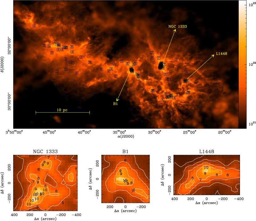
Figure 1: Sampling of the Perseus cloud. Top: H₂ column density map of the Perseus molecular cloud from Zari et al. (2016) with squares indicating the location of the 100 positions selected to characterize the line emission from the cloud using stratified random sampling. The number in each square indicates the column density bin to which the position belongs, and ranges from 1 (lowest column density) to 10 (highest). Bottom: Expanded view of the three regions that concentrate most of the high column density positions, and that correspond to the well-known star-forming regions NGC 1333, B1, and L1448. Contours are in units of $N$(H₂), start at $1.25\times 10^{21}$ cm^-2, and increase by factors of 2.5. The 10 pc scale bar assumes a distance of 300 pc.

The goal of our work is to sample the different regimes of the cloud molecular emission using a relatively small number of positions, even if the cloud emission properties are not initially well known. Choosing positions at random does not seem like a good strategy, since a typical cloud has so many more positions with weak emission that the probability of randomly picking bright positions is negligibly low (Rosolowsky et al., 2008b).

A better option is to guide the choice of positions by a proxy that is expected to correlate with the molecular emission. A natural choice for this proxy is the H₂ column density, which has been shown by principal component analysis to have a dominant contribution to the emission of some clouds (Ungerechts et al., 1997; Gratier et al., 2017). The H₂ column density, in addition, can be determined with accuracy over entire molecular clouds using a combination of dust extinction and emission measurements (e.g., Lombardi et al. 2014). For the Perseus cloud, Zari et al. (2016) have recently determined the distribution of H₂ column density combining dust emission data from the Herschel and Planck satellites together with NIR dust extinction measurements from the 2MASS survey. This determination covers the full extent of the cloud and has a dynamic range of about two orders of magnitude. In addition, it has an angular resolution of $36^{\prime\prime}$, which is similar to what is currently achievable with single-dish radio telescopes.

To sample the cloud using the H₂ column density as a proxy, we need to sample the distribution of H₂ column densities in the cloud so that each column density regime is well represented. Properly sampling this distribution, however, requires some care since, like the emission, the population of column densities is overwhelmingly dominated by the positions with the lowest values. Zari et al. (2016) found that the probability distribution function of the column density follows a power law with a slope of $-3$, and as a result, that the number of positions at the low end of the distribution ($N(\mathrm{H}_{2})\approx 10^{21}$ cm^-2) exceeds the number of positions at the high end ($N(\mathrm{H}_{2})\approx 10^{23}$ cm^-2) by about six orders of magnitude (Fig. 8 in Zari et al. 2016). Sampling the distribution by choosing positions with random column density is therefore impractical since it would require selecting about one million samples to ensure that the full range of column densities is covered.

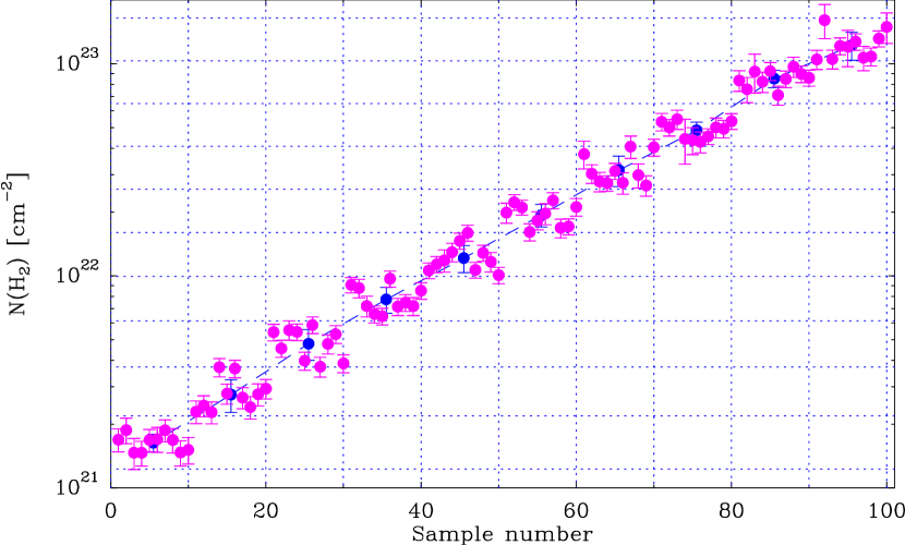
Figure 2: H₂ column density as a function of sample number for the 100 positions randomly chosen to represent the Perseus molecular cloud (magenta circles). The dashed horizontal lines mark the boundaries of the ten column-density bins in which the cloud was divided, and the vertical lines enclose the ten points chosen to sample each bin. The blue circles indicate the geometrical mean of the H₂ column densities inside each bin, and their error bars indicate their dispersion. All values derived from Zari et al. (2016) data.

A more practical approach is to first identify the different column density regimes in the cloud and then to sample each regime by choosing a number of cloud positions at random. This sampling approach is an instance of the “stratified random sampling” technique often used in surveys (Cochran, 1977), and whose name derives from the word “strata” used to denote the different subpopulations of the sample, which in our case correspond to the column density regimes of the cloud.

Since the distribution of column densities in Perseus follows a power law over the approximately two orders of magnitude for which the extinction measurements are reliable ($1.5\times 10^{21}$ ¡ $N$(H₂) ¡ $1.5\times 10^{23}$ cm^-2, corresponding to 0.2 ¡ $A_{\mathrm{K}}$ ¡ 20 mag, Zari et al. 2016), we chose to bin this range using logarithmically spaced column-density intervals. The width of these intervals was taken as 0.2 dex, equivalent to a factor of 1.6 in column density, with the expectation that the molecular emission will not change dramatically (more than a factor of 2) between the bins. As shown below, this expectation is satisfied over most of the cloud, although it seems to break down toward the lowest column density bin ($A_{\mathrm{V}}\approx 1-2$ mag), where the emission often drops precipitously due to photodissociation at the cloud edge. Our column density sampling is clearly not fine enough to resolve the details of the cloud boundary, but seems to work well over the rest of the cloud. Since the cloud column density range spans two orders of magnitude, a choice of a 0.2 dex interval resulted in a total of ten logarithmically spaced column-density bins.

In standard applications of the stratified sampling method, the strata are sampled proportionally to their population. As mentioned above, this approach is impractical when sampling the column density bins of Perseus (or any other cloud) because their populations can differ by multiple orders of magnitude. As an expedient solution motivated by the limited observing time available, we chose to sample each bin using the same number of positions, which we took as ten. This number was chosen as a compromise between the competing needs of observing enough positions per bin to determine with some accuracy the mean and the dispersion of the intensity, and the need to make long enough integrations to detect the weak emission of the positions in the lowest column density bins. Since the success of this sampling strategy depends strongly on the intensity and the dispersion of the emission inside the bins, which was not known before the observations, our choice of sampling parameters should be taken only as a tentative initial approach. A proper optimization of the stratified random sampling technique to characterize molecular clouds is still needed to assess a number of possible weaknesses of our approach, which include the use of limited sampling in the very extended low column density bins (which could lead to statistical fluctuations) and the use of H₂ column density as the sole guide to sample the cloud emission to the exclusion of other parameters, such as the gas temperature or the star-formation activity. Carrying out this investigation requires having full maps of clouds in a variety of molecular tracers, which fortunately is now becoming possible thanks to the efforts of dedicated observing programs such as ORION-B (Pety et al., 2017) and LEGO (Barnes et al., 2020).

Once the number of sampling positions had been determined, the practical choice of selecting them at random was done by first identifying all the pixels in the extinction map of Zari et al. (2016) that belong to each column density bin. These pixels were listed in a table, and ten of them were selected by repeatedly drawing random numbers uniformly distributed between one and the number of pixels in the bin. Table 4 presents a list with the coordinates of the resulting 100 cloud positions. Their relative location inside the cloud is shown in Fig. 1.

To illustrate the two orders of magnitude in H₂ column density covered by the sample, Fig. 2 shows the value determined using the prescription from Zari et al. 2016 for each sample position (magenta symbols). Each column density bin is enclosed between dashed horizontal lines, and as expected, the points inside each bin are distributed randomly in column density. The figure also shows the geometrical mean and dispersion inside each bin (blue symbols). We note that the error bars in the individual column densities are typically smaller than the dispersion inside the bins, although an additional source of uncertainty in the column density arises from the particular choice of extinction per H atom assumed by Zari et al. (2016), which could shift the estimates globally by a factor of up to about 1.5 depending on the true dust properties (Fig. 2 in Draine 2003).

3 Observations

We observed our sample of Perseus positions using the Institut de Radioastronomie Millimétrique (IRAM) 30m-diameter telescope in Pico Veleta (Spain) during three runs in June 2017, September 2017, and January 2018. In the first two runs, the 3mm channel of the Eight MIxer Receiver (EMIR, Carter et al. 2012) was used to observe the full frequency range from 83.7 and 115.8 GHz (telescope FWHM of $29^{\prime\prime}$ to $21^{\prime\prime}$). These observations used the facility fast Fourier Transform Spectrometer (FTS, Klein et al. 2012), which was configured to cover the receiver instantaneous passband with a frequency resolution of 200 kHz ($\approx 0.6$ km s^-1).

For all positions, the integration time was approximately 10 minutes after combining the two linear polarizations, except for the positions in the lower column density bin, which were observed twice as long to compensate for their weaker lines. Additional observations of 33 positions from our sample were carried out using simultaneously the 3mm and 2mm channels of EMIR and covering two narrow frequency ranges centered on HCO⁺(1–0) and CS(3–2). These observations had the goal of obtaining high velocity resolution spectra, and used as a backend the Versatile SPectrometer Array (VESPA) with a frequency resolution of 20 kHz ($\approx 0.06$ km s^-1).

In the last observing run (January 2018), we used the 1mm channel of the EMIR receiver to observe four frequency windows within the range 213.7-267.7 GHz (telescope FWHM of $11^{\prime\prime}$-$9^{\prime\prime}$). These windows were selected for containing higher-$J$ transitions of some 3mm target lines, such as CO(2–1), HCN(3–2), and CS(5–4). Again, the FTS backend was used to cover as much passband as possible with a frequency resolution of 200 kHz, equivalent to $\approx 0.25$ km s^-1 at the frequency of operation. Since the 1mm lines are weaker than those at 3mm, the lowest three column density bins of the sample were not fully observed, and the integration time per point typically ranged between 10 and 40 minutes (after combining polarizations), depending on the strength of the line.

All observations were carried out in frequency switching mode with symmetric offsets of $\pm 7.7$ MHz. Atmospheric calibration was performed every 10-15 minutes using the standard sky-ambient-cold load cycle, and the telescope pointing and focus were checked and corrected every two hours approximately. The resulting folded spectra were further processed using the CLASS program, with which repeated observations and overlapping frequency windows were STITCHed together. Polynomial baselines were used to remove ripples in the passband, and the intensity was converted to the main beam brightness scale using the facility-provided telescope efficiencies. Typical rms in the spectra range from 6 to 9 mK per 0.6 km s^-1 channel at 100 GHz.

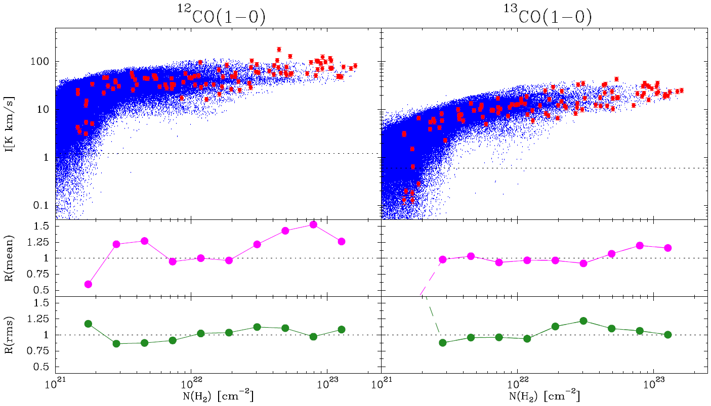
Figure 3: Comparison between sampling observations and COMPLETE full maps for ¹²CO(1–0) and ¹³CO(1–0). Top panels: Scatter plots of the integrated intensity as a function of $N$(H₂). The blue dots represent the results from the COMPLETE maps presented by Ridge et al. (2006) and each of them contains more than $2\times 10^{5}$ spectra. The red symbols represent the 100 measurements obtained using stratified random sampling. The dotted lines mark the $3\sigma$ detection level of the COMPLETE maps. Middle panels: Ratio between the mean intensity derived using the sampling data and the COMPLETE maps for each of the ten $N$(H₂) bins in which the cloud was divided. For ¹³CO(1–0), the measurement in lowest $N$(H₂) bin is not reliable since the sampling data show that the intensity often lies below the COMPLETE detection limit. Bottom panels: Ratio between the rms derived using the sampling data and the COMPLETE maps. As with the mean values, the ¹³CO(1–0) measurement for the lowest $N$(H₂) bin lies below the detection limit, so the rms estimate is not reliable. We note how both the mean and rms ratios for the two CO isotopologs lie in the vicinity of 1, indicating that the sampling method allows estimating the main emission parameters with an accuracy of about 50-20% depending on the parameter.

In most of the following analysis, we rely on the integrated intensity of the different molecular lines. These intensities were estimated from the reduced spectra by integrating the emission over the velocity channels where a visual inspection showed signal. For spectra with no clear signal, the intensity was estimated by integrating the emission inside the velocity range where the ¹³CO(1–0) line was detected since this abundant species was identified toward almost all cloud positions, and its velocity range was found to coincide with that of all the other lines in case of mutual detection. The uncertainty of each integrated intensity was estimated from the rms level of the spectrum. Following previous IRAM 30m studies, we added in quadrature a 10% calibration error to include uncertainties in the beam efficiencies and day-to-day variations (Pety et al., 2017; Jiménez-Donaire et al., 2019). Table 4 summarizes the derived intensities.

4 Survey results

4.1 Comparison with the COMPLETE project

Before analyzing the data, we test how well our sampling observations recover the main properties of the cloud emission. For this, we compare our ¹²CO(1–0) and ¹³CO(1–0) intensities with the results from the Coordinated Molecular Probe Line Extinction and Thermal Emission (COMPLETE) project, which mapped the entire Perseus cloud in ¹²CO(1–0) and ¹³CO(1–0) using the FCRAO 14m telescope. These data have been presented by Ridge et al. (2006), and their correlation with the extinction determined using 2MASS data has been studied in detail by Pineda et al. (2008) and Goodman et al. (2009). To compare our survey data with the COMPLETE results, we first converted the COMPLETE intensities into the main beam brightness scale using the efficiencies recommended by Ridge et al. (2006). We then resampled the extinction map from Zari et al. (2016) to the same spatial grid used by COMPLETE, in order to obtain for each position of the COMPLETE map an estimate of the H₂ column density $N$(H₂). This estimate was determined from the extinction data using the conversion factors recommended by Zari et al. (2016).

In the top panels of Fig. 3, we represent the intensity of the ¹²CO(1–0) and ¹³CO(1–0) lines as a function of the H₂ column density for both the sampling and COMPLETE datasets. This type of plots constitutes the basis of most of our Perseus analysis presented below, so it represents the most adequate tool to perform the data comparison. The COMPLETE data are represented with blue symbols and consist of more than $2\times 10^{5}$ points, one for each spectrum used to generate each COMPLETE map (Ridge et al., 2006). Superposed with red circles, we present the results from our sampling observations, also in main-beam brightness temperature scale and with the H₂ column density estimated using the Zari et al. (2016) prescription.

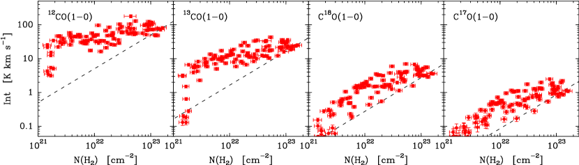
Figure 4: Integrated line intensity as a function of H₂ column density for the $J$=1–0 transition of the four main CO isotopologs. For reference, each panel shows a linear relation that fits the average intensity of the highest column density bin (dashed line). Depending on the transition, the lower limit of the intensity scale (0.05 K km s^-1) approximately corresponds to one to three times the noise level in the integrated intensity.

As Fig. 3 shows, the distribution of the COMPLETE and sampling points agree both in their correlation with $N$(H₂) and in the amount of dispersion for a given $N$(H₂), indicating that the sampling observations recover the general trends of the emission from the full cloud. There seems to be a slightly better agreement between the sampling and the COMPLETE results for the ¹³CO(1–0) data, although its cause is unclear since both CO isotopologs were observed simultaneously by the two surveys. We note that small discrepancies between the data are unavoidable given their different calibrations and the factor of two difference in angular resolution between the IRAM 30m telescope used in our sampling survey ($\approx 21^{\prime\prime}$) and the FCRAO 14m telescope used in COMPLETE ($\approx 46^{\prime\prime}$).

To quantify the comparison between the sampling and the COMPLETE results, we calculated for each dataset the intensity mean and rms inside each of the ten column density bins in which we have divided the cloud. Given the large dispersion of the data, we operated in logarithmic units and later converted the results to a linear scale. The results of this calculation are shown in the middle and bottom panels of Fig. 3 in the form of ratios between the estimates derived using the sampling method and the COMPLETE maps.

As expected from the scatter plots, the sampling/COMPLETE ratio of the means (middle panels) is close to unity over the full range of $N$(H₂) for both CO isotopologs. The largest deviations from unity occur in ¹²CO(1–0), but they reach at most a factor of about 1.5 and do not show any systematic pattern of bias. Also as expected from the scatter plots, the ¹³CO(1–0) ratios are better behaved, and our estimate indicates an agreement between the sampling and the COMPLETE mean values at the level of 25%. The only disagreement between the ¹³CO(1–0) sampling and COMPLETE results occurs in the lowest column density bin ($N(\mathrm{H}_{2})<2.2\times 10^{21}$ cm^-2), where some of the line intensities measured with the sampling technique lie below the three sigma detection level of the COMPLETE data (dotted line in the scatter plots). This suggests that the COMPLETE data are too shallow to characterize the ¹³CO(1–0) intensity in the lowest column density bin, and as a result, they artificially overestimate the mean value and underestimate the dispersion.

Even better agreement between the sampling and the COMPLETE results is found for the estimate of the emission rms. As shown in the bottom panels of Fig. 3, the ¹²CO(1–0) data agree better than 25%, although the sampling method can barely follow the large rms increase in the lowest column density bin seen in the upper panel. In hindsight, having observed additional positions in this bin would have been desirable. For ¹³CO(1–0), the agreement between sampling and mapping results is also better than 25%, again excluding the lowest column density bin due to the insufficient sensitivity of the shallower COMPLETE data.

To summarize, a comparison with the COMPLETE mapping data suggests that the stratified random sampling method can provide estimates of the intensity mean and dispersion that have an accuracy of better than a factor of 1.5, and are usually at the 20% level, for the whole range of column densities covered by our survey. This comparison is unfortunately limited to CO data since this is the only species for which large-scale maps are available. While further testing is needed using different species (and clouds), the results obtained so far support the idea that stratified random sampling is a potentially useful tool to efficiently determine the global properties of the cloud emission.

4.2 Data overview

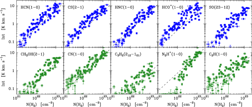
Figure 5: Integrated line intensity as a function of H₂ column density for the survey species detected in at least five column density bins. Top: Traditional dense gas tracers (blue symbols). Bottom: Additional tracers of dense gas (green symbols). For reference, each panel shows a linear relation that fits the average intensity of the highest column density bin (dashed line). For HCN(1–0), CN(1–0), N₂H⁺(1–0), and C₂H(1–0), the intensity includes the contribution from all detected hyperfine components. For CH₃OH(2–1), the intensity includes the contribution from the A⁺ and E components. Depending on the transition, the lower limit of the intensity scale (0.05 K km s^-1) approximately corresponds to one to three times the noise level in the integrated intensity.

The number of molecular lines detected in each position depends strongly on its column density. Toward positions with the highest column densities (bin number 10, with $N$(H₂) $\geq 10^{23}$ cm^-2), the spectra contain about 50 different molecular lines in the 3mm band alone. As the column density decreases, the number of detected lines decreases rapidly, and in the lowest column density bin ($N$(H₂) $\approx 10^{21}$ cm^-2), the detections are often limited to the lines of the abundant CO isotopologs. Since our goal is to study the dependence of the line intensity with the gas column density, we restrict our analysis to those 3mm lines that are detected in most positions belonging to at least five column density bins out of the ten in which we divided the cloud. In this section, we focus our discussion on these brighter lines that satisfy our selection criterion. Table 4 presents their integrated intensity estimated, as described in Sect. 3, by integrating the emission over the range of detection, and in case of non detection, by integrating the emission over the range at which ¹³CO(1–0) was detected. Appendix B illustrates the data presenting stacked spectra of all 3mm transitions for each column density bin.

For presentation convenience, we have divided these lines into three different chemical families. The first chemical family is that of the CO isotopologs, and consists of ¹²CO, ¹³CO, C¹⁸O, and C¹⁷O. Fig. 4 shows the velocity-integrated intensity of their $J$=1–0 transition as a function of H₂ column density. As shown below, the results for the $J$=2–1 line are almost indistinguishable from those of the $J$=1–0, so we can safely base our analysis on the low-energy transition. For reference, each plot contains a dashed line showing a linear relation that would fit the mean intensity of the highest column density bin.

The most noticeable trend in Fig. 4 is the strong correlation between all the line intensities and the H₂ column density over the two orders of magnitude that this parameter spans across the sample. Since the sample positions in each column density bin are located randomly over the cloud, this correlation indicates that the H₂ column density is by itself a strong predictor of the CO line intensity, a first hint that our reliance on the H₂ column density as a proxy for the line emission is an acceptable choice.

As Fig. 4 shows, the brighter ¹²CO and ¹³CO lines have the largest dynamic range, and their distribution with H₂ column density presents an abrupt change in slope at around $2\times 10^{21}$ cm^-2 ($A_{\mathrm{V}}\approx 2$ mag). This change has been previously characterized by Pineda et al. (2008), who used data from the COMPLETE survey to study the intensity of the CO isotopologs in Perseus as a function of extinction for $A_{\mathrm{V}}<10$ mag (equivalent to $N$(H₂) $<10^{22}$ cm^-2). It likely results from the photodissociation of the CO molecules in the outer cloud by the UV photons from the external interstellar radiation field (e.g., Tielens & Hollenbach 1985; van Dishoeck & Black 1988; Le Bourlot et al. 1993; Sternberg & Dalgarno 1995; Visser et al. 2009; Wolfire et al. 2010; Joblin et al. 2018). Inner to the photodissociation edge, the slope of the ¹²CO and ¹³CO intensities is relatively flat compared with the linear slope, a trend that will be shown below to result from saturation effects, in agreement with the previous suggestion from Pineda et al. (2008).

For the C¹⁸O and C¹⁷O lines, the photodissociation edge is not appreciable at low column densities due to insufficient sensitivity, although it can be hinted in the bin-averaged data discussed below. As the column density increases, the C¹⁸O and C¹⁷O intensities increase almost linearly with $N$(H₂) up to about $10^{22}$ cm^-2, and then flatten significantly at higher column densities. This flattening is not caused by optical depth effects since the C¹⁸O(1–0)/C¹⁷O(1–0) ratio has a close-to-constant value of $3.2\pm 0.1$, which matches the ¹⁸O/¹⁷O isotopic ratio found for the ISM by Wilson & Rood (1994), indicating that both the C¹⁸O(1–0) and C¹⁷O(1–0) lines are optically thin over the entire Perseus cloud. As shown by the cloud model discussed below, the flattening is likely caused by the freeze out of the CO molecules onto the dust grains at the high densities characteristic of the regions with high $N$(H₂).

The other two families in which we divide the species detected in our survey are presented in Fig. 5. The top row of panels shows species that are commonly used to trace dense gas both in galactic and extra-galactic studies, such as HCN, CS, HNC, HCO⁺, and SO (e.g., Evans 1999; Kennicutt & Evans 2012). We will refer to these species collectively as “traditional dense gas tracers,” with the caveat that their role as true dense gas tracers is being reassessed as a result of recent work (Kauffmann et al. 2017, Pety et al. 2017, Shimajiri et al. 2017, see further discussion in Sect. 6.2). The bottom row contains a more heterogeneous mix of species. Most of them are sensitive to dense gas, but they often present strong sensitivity to additional processes such as shocks, UV radiation, or CO freeze out: CH₃OH, CN, C₃H₂, N₂H⁺, and C₂H (van Dishoeck & Blake, 1998; Bergin & Tafalla, 2007). We will refer to this group of species as the “additional tracers” family for lack of a better term.

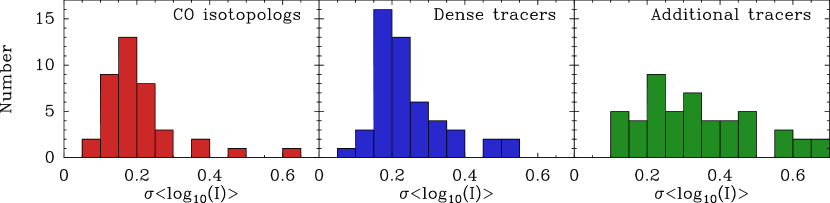
Figure 6: Dispersion histograms of logarithmic intensity for each column density bin. The panels show the combined dispersion for the family of CO isotopologs (left), the traditional dense gas tracers (middle), and the additional tracers (right). In all cases, the lowest column density bin has been excluded due to low sensitivity.

As with the CO isotopologs, the intensity of the traditional dense gas tracers presents a strong correlation with the H₂ column density over the two orders of magnitude sampled by the survey. The lower signal-to-noise ratio of these tracers at low H₂ column density makes it difficult to judge whether they present a photodissociation edge similar to that of CO, although there are hints of such an edge at least in the HCN data. Better evidence for photodissociation edges in some of these tracers will be presented in Sect. 4.4 when we analyze the bin-averaged data.

Inside the photodissociation edge, all traditional dense gas tracers present a clear quasi-linear correlation with $N$(H₂), as indicated by the good match between the data points and the linear dashed lines. This systematic behavior of the traditional dense gas tracers is somewhat unexpected since common belief among observers suggests that a linear correlation with column density would only be expected for the thermalized lines of the thin CO isotopologs. The traditional dense gas tracers, due to their subthermal excitation, are expected to trace volume density, not column density, and therefore present a steeper intensity slope. Understanding this unexpected behavior requires a detailed modeling of the cloud physical and chemical properties, which we defer to Sect. 6.1 below. Here we only stress that the remarkable linear behavior extends over the two orders of magnitude in H₂ column density covered by the observations.

The set of additional tracers, shown in the bottom row of Fig. 5 presents a more diverse behavior in their dependence with the H₂ column density. This behavior ranges from the close to linear correlation of CH₃OH to the significantly nonlinear behavior of N₂H⁺, whose intensity drops precipitously at H₂ column densities below $10^{22}$ cm^-2. Less notable, but still significant, are the deviations from linearity seen in CN and C₂H, whose intensities increase slightly but significantly (factors of two or three) over the linear trend for column densities lower than $10^{22}$ cm^-2. The possible origin of all these behaviors is explored below with the help of a radiative-transfer cloud model.

4.3 Data dispersion

As mentioned above, the intensity of each line in the survey correlates strongly with the H₂ column density, indicating that despite the random location of the observed positions, their line intensity can be accurately predicted from the value of $N$(H₂). This result is important for the use of the stratified random sampling method since, as discussed in Sect. 2, it requires that the H₂ column density is a reliable proxy for the molecular emission. To better quantify how well the H₂ column density predicts the intensity of each line, we have studied the dispersion of the intensities inside each column density bin.

For each transition, we calculated the mean and rms dispersion of the ten intensity values belonging to each column density bin. Since the observations in the lowest column density bin often resulted in non detections (likely due to low sensitivity and photodissociation effects), we ignored this bin in our dispersion calculations. In Fig. 6, we present histograms of the log-scale rms dispersion inside each column density bin for the three chemical families defined before.

As can be seen, the rms dispersion of the CO isotopologs and the traditional dense gas tracers has a well-defined peak near 0.2 dex, a result that does not change if we include the data from the lowest column density bins. This level of dispersion is equivalent to a factor of 1.6 in linear scale, and its small value is responsible for the tight correlations that characterize the intensity-column-density plots. While low, the dispersion in the intensities is significantly higher than the dispersion of column densities inside each bin, which we estimate as 0.05 dex. This indicates that the scatter of intensities is intrinsic to the gas, and not a mere reflection of the range of column densities contained inside each bin.

As Fig. 6 shows, the family of additional tracers presents a wider distribution of dispersions and lacks a clear peak, in agreement with the diversity of scatter levels seen in the bottom row of Fig. 5. The mean value of this distribution is 0.3 dex, again independently of whether the lowest column density bin is included. This value implies that the intensities in this chemical family have an rms scatter of a factor of two in linear scale, which is still much smaller than the two orders of magnitude spanned by the intensities. This again reflects the significant correlation between line intensities and H₂ column densities.

While the low scatter of the intensities supports the use of the column density as a proxy for the stratified random sampling, the fact that the scatter exceeds what would be expected simply from column density variations indicates that the column density is not a perfect predictor of the emergent intensity. This should not be surprising given that the column density is an integrated quantity that can be realized by multiple physical and chemical conditions along the line of sight. Our data already suggest several contributions to the dispersion of intensities associated with a single column density. Chemical effects, for example, likely play a role in the higher dispersion seen in the lines of C₃H₂ and C₂H. These two species are known to present similar sensitivity to the presence of an external radiation field (Pety et al., 2005), and this field likely changes significantly across the cloud. Optical depth effects, in addition, are likely to contribute to the dispersion of intensities seen in species like HCO⁺(1–0), whose scatter is significantly larger toward the high column density bins. Observations of this line at selected positions using high velocity resolution reveal that the HCO⁺(1–0) lines often suffer from self absorption, a fact confirmed by the data from the optically thinner H¹³CO⁺(1–0), shown in Appendix D, which present a much lower degree of scatter. Another contribution to the scatter in the line intensities comes from differences in the distribution of densities (and possible temperatures) along each line of sight. This is suggested by an observed increase in the scatter of the HCN and CS lines as their level energy increases (Sect. 5). Higher $J$ lines have higher critical densities, and are therefore more sensitive to density variations along the line of sight. While the above examples show the intrinsic limitation of using column density as the sole predictor of the emergent intensity, they also illustrate how further understanding of the emission scatter could provide new insights on the internal structure of molecular clouds.

4.4 Correlation with H₂ column density

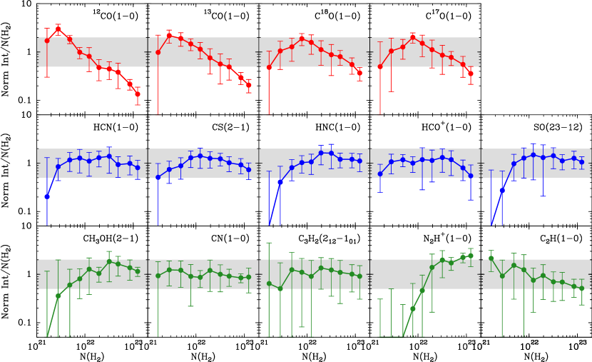
Figure 7: Normalized ratio between integrated intensity and H₂ column density as a function of H₂ column density. The data points represent bin-averaged values and the error bars represent the rms dispersion. The horizontal gray band encloses the region were deviations from unity are within a factor of 2.

Table 1: Linear square fits to the $\log$-$Int$ vs. $\log$-$N$(H₂) plots.

Transition	Slope	Pearson-$r$
CO isotopologs
12CO($J$=1–0)	$0.37\pm 0.04$	0.70
13CO($J$=1–0)	$0.62\pm 0.06$	0.73
C18O($J$=1–0)	$0.82\pm 0.05$	0.86
C17O($J$=1–0)	$0.71\pm 0.04$	0.87
Traditional dense gas tracers
HCN($J$=1–0)	$0.99\pm 0.04$	0.93
CS($J$=2–1)	$1.13\pm 0.05$	0.93
HNC($J$=1–0)	$1.18\pm 0.04$	0.94
HCO+($J$=1–0)	$0.97\pm 0.05$	0.88
SO($N,J$=23–12)	$1.17\pm 0.06$	0.90
Additional tracers
CH3OH($J_{k}$=2–1)	$1.30\pm 0.07$	0.90
CN($N$=1–0)	$0.90\pm 0.04$	0.93
C3H2($J_{Ka,Kc}$=212–101)	$0.87\pm 0.07$	0.81
N2H+($J$=1–0)	$1.76\pm 0.08$	0.93
C2H($N$=1–0)	$0.78\pm 0.06$	0.78

To quantify how linear the dependence of the intensity with $N$(H₂) is, we made least squares fits to the data points in Figs. 4 and 5 (in log-log scale). To avoid any possible effect of the photodissociation edge, we excluded the data in the first column density bin, and for N₂H⁺, we also excluded the data in the following three bins because no emission was detected in them. Table 1 presents the fit results (in log-log) together with the Pearson $r$ coefficient for all the transitions.

As expected from the diagrams, the CO isotopologs present slopes that are significantly lower than one, which is the value that corresponds to a linear correlation. The lowest slope values are those of ¹²CO and ¹³CO, and reflect the high optical depth of these lines, which makes their emission only weakly dependent on the gas column density. The lines from the rare isotopologs C¹⁸O and C¹⁷O are optically thin and present higher slope values. Still, their lower-than-one slopes indicate that the lack of a linear correlation between the intensity and the H₂ column density represents an intrinsic property of the CO emission.

Also as expected from the scatter plots, the slopes derived for the traditional dense gas tracers are very close to unity. The slope values in Table 1 range between 1.0 to 1.2, and have a scatter at the level of about 5%. In addition, the Pearson $r$ coefficients of these tracers have similar values of about 0.9 indicative of a strong level of correlation.

Most members of the additional tracers group have slope values similar to those of the traditional dense gas tracers, but a few deviate noticeably from a linear behavior. The most clear case is N₂H⁺, which has a slope of 1.76 indicative of a preference for high column densities. More marginal, but probably still significant, is the case of CH₃OH, which has a slope of 1.30. At the other end of the scale, C₂H presents a significantly flat slope of 0.78, indicative of a slight intensity increase toward the low column density gas.

A more graphic representation of the close-to-linear relation between some of the line intensities with $N$(H₂ ) is presented in Fig. 7. This figure shows the ratio between the line intensity and the H₂ column density for each selected transition. For clarity, the plot shows normalized ratios with error bars that indicate the data dispersion inside each bin.

The top panels in Fig. 7 (red symbols) show how the CO isotopologs significantly deviate from the constant ratio that corresponds to a linear correlation between intensity and column density. This deviation is largest in the optically thick lines of ¹²CO and ¹³CO, whose ratio with the H₂ column density varies by more than one order of magnitude over the cloud range. The thinner C¹⁸O and C¹⁷O lines also present non constant ratios, but the variation of their geometrical mean over the cloud is limited to a factor of two up and down, a range that is indicated with a gray-shaded band. As mentioned above, the emission from these two isotopologs is optically thin, so the curvature in the plots of Fig. 7 likely arises from systematic variations of the molecular abundance inside the cloud, an interpretation that will be further explored with a radiative transfer model in Sect. 5.

The middle panels in Fig. 7 (blue symbols) show the behavior of the intensity-column density ratio for the traditional dense gas tracers. Overall, these tracers behave more linearly than the CO isotopologs, and most of their data points lie inside the gray-shaded band that encloses variations within a factor of 2. There is marginal evidence that in most tracers the point from the lowest column density bin lays below the gray-shaded band, with the possible exception of HCO⁺. The most likely cause of this drop is the photodissociation of molecules by the external UV radiation field.

Finally, the bottom panels in Fig. 7 present the results for the additional tracers (green symbols). Most of these tracers have ratios inside the gray-shaded band, with the clear exception of N₂H⁺ and possibly CH₃OH. The sudden drop of N₂H⁺ at H₂ column densities lower than $2\times 10^{22}$ cm^-2 is highly significant since the observations had enough sensitivity to detect this species at low column densities if the intensity had continued the linear trend. As it will be discussed in the Sect. 5, the drop is consistent with the N₂H⁺ abundance being only significant in the denser regions of the cloud where CO is frozen out on the grains, as previously indicated by observations of dense cores (Caselli et al., 1999; Bergin et al., 2002; Tafalla et al., 2002).

Although the data points of C₂H remain in the gray-shaded band of Fig. 7, they present a gradual increase by a factor of four from high to low column densities. This increase is again consistent with the expected abundance enhancement of C₂H toward the outer cloud caused by the external UV radiation field (Pety et al., 2005). The related species CN does not present a noticeable increase, although the detailed model of the intensities below shows that it may be slightly enhanced toward the outer cloud.

To conclude the discussion, we provide in Table 2 estimates of the $X$-factor (defined as the H₂ column density over line intensity) for each line of the dense-gas and additional tracers as derived from our least-squares fit. For all species except for N₂H⁺, data from all the column density bins but the lowest one were used in the fit. For N₂H⁺, the fit used data only from the highest four column density bins since the emission of this species drops non linearly at lower column densities. Given the approximate linear behavior of all the tracers, the $X$-factors in the table could be used to compare the intensity of the Perseus emission with that of other clouds. They could also be used to infer H₂ column densities from the intensity of the observed lines, although without a proper calibration using other clouds, the result will be subject to a great degree of uncertainty.

Table 2: $X$-factors for high-dipole moment species.

Transition	$X$	Transition	$X$
HCN(1–0)	$1.2\times 10^{22}$	CH3OH(2–1)	$3.6\times 10^{22}$
CS(2–1)	$1.3\times 10^{22}$	CN(1–0)	$1.2\times 10^{22}$
HNC(1–0)	$2.1\times 10^{22}$	C3H2(212–101)	$1.1\times 10^{23}$
HCO+(1–0)	$1.2\times 10^{22}$	N2H+(1–0)	$1.4\times 10^{22}$
SO(23–12)	$2.5\times 10^{22}$	C2H(1–0)	$2.2\times 10^{22}$

4.5 Comparison with other clouds

As mentioned in the Introduction, a recent effort has been made by different authors to map the emission of entire or close-to-entire molecular clouds in multiple lines. In this section we compare the results from this effort to our observations, both to test the sampling technique and to study the behavior of the emission in different molecular clouds.

We first compare our dataset with that of Watanabe et al. (2017), who carried out a multiline study of the high-mass star-forming cloud W51. These authors found that the 3mm-wavelength emission from W51 is dominated by the lines of the CO isotopologs together with the same traditional dense gas tracers found by us in Perseus (HCN, HCO⁺, HNC, and CS). Lacking extinction measurements for W51, Watanabe et al. (2017) used the integrated intensity of ¹³CO(1–0) as a proxy for the cloud column density, and found a tight and often close-to-linear correlation between this tracer and the integrated intensity of most molecular lines. This result is similar to our finding of a tight correlation between the intensity of the main molecular species and the H₂ column density in Perseus, with the caveat that in Perseus the ¹³CO(1–0) emission does not correlate linearly with the H₂ column density (although in contrast with Perseus, the ¹³CO(1–0) emission in W51 is optically thin, see Watanabe et al. 2017).

A better comparison to our work can be made with the large-scale mapping of Orion B by Pety et al. (2017). These authors used extinction measurements from Lombardi et al. (2014) to study the correlation between the intensity of the different lines and the extinction, as we have done with the Perseus data. In good agreement with our results, these authors find a tight correlation that is often close to linear for column densities larger than a threshold value equivalent to an extinction of $A_{\mathrm{V}}$=1-3 mag (their Fig. 10).

Further insight on the Orion B molecular emission comes from the principal component analysis of Gratier et al. (2017) using the same dataset as Pety et al. (2017). This analysis shows again that the main predictor of the cloud emission is the gas column density, which is responsible for the first principal component (60 % contribution). The following principal components (at the 10 % level) reveal several species whose emission presents a peculiar behavior: N₂H⁺ and CH₃OH, classified as sensitive to gas density, and C₂H and CN, classified as sensitive to UV. These species are the same as those identified as peculiar in Perseus (Sect. 4.4), and this common behavior suggests that despite their very different characteristics (Orion B contains several embedded HII regions and the bright Horsehead PDR), the molecular emission from these two clouds is controlled by the same main mechanisms.

The final dataset with which we compare our Perseus results is that presented by Kauffmann et al. (2017) for Orion A, which is more limited than our Perseus dataset in number of transitions. Kauffmann et al. (2017) focus their study of dense gas tracers on HCN, CN, C₂H, and N₂H⁺, which are four of the 11 species we studied in Perseus. For the first three species, they find that the ratio of the integrated intensity over the gas column density varies little over the cloud, and decreases at most by a factor of two when the column density increases by one order of magnitude (their Fig. 2). This behavior is similar to the almost constant intensity-column density ratio found by us in Perseus.

Also in agreement with our Perseus results, the N₂H⁺ emission from Orion A differs from the other tracers by increasing rapidly in the most opaque gas (with the possible exception of the densest two bins). As Kauffmann et al. (2017) discuss, the N₂H⁺ emission seems to be the only tracer that is sensitive to the densest component of the cloud.

While limited in targets, the above studies and our Perseus data cover a variety of clouds with different levels of star-formation activity both in the low and high-mass regimes. Despite these differences, all clouds present systematic and often tight correlations between the emission from most molecular tracers and the gas H₂ column density. This correlation indicates that the cloud H₂ column density behaves as a reliable proxy of the molecular emission under a variety of cloud conditions, which we saw was a requirement for the stratified sampling method to work. The data, therefore, support the idea that the stratified sampling method could be used to characterize the emission from a large variety of clouds.

The data also show that there are significant similarities between the emission from the different clouds, both in terms of the brightest lines and the dependence of their intensity with the H₂ column density. Clearly more work needs to be done in this area, especially by comparing clouds using the same observing technique. The initial results, however, suggest that despite the large differences between the clouds in terms of mass and star-formation activity, the emission that they produce follows a relatively simple and similar pattern.

5 A simple emission model for the Perseus cloud

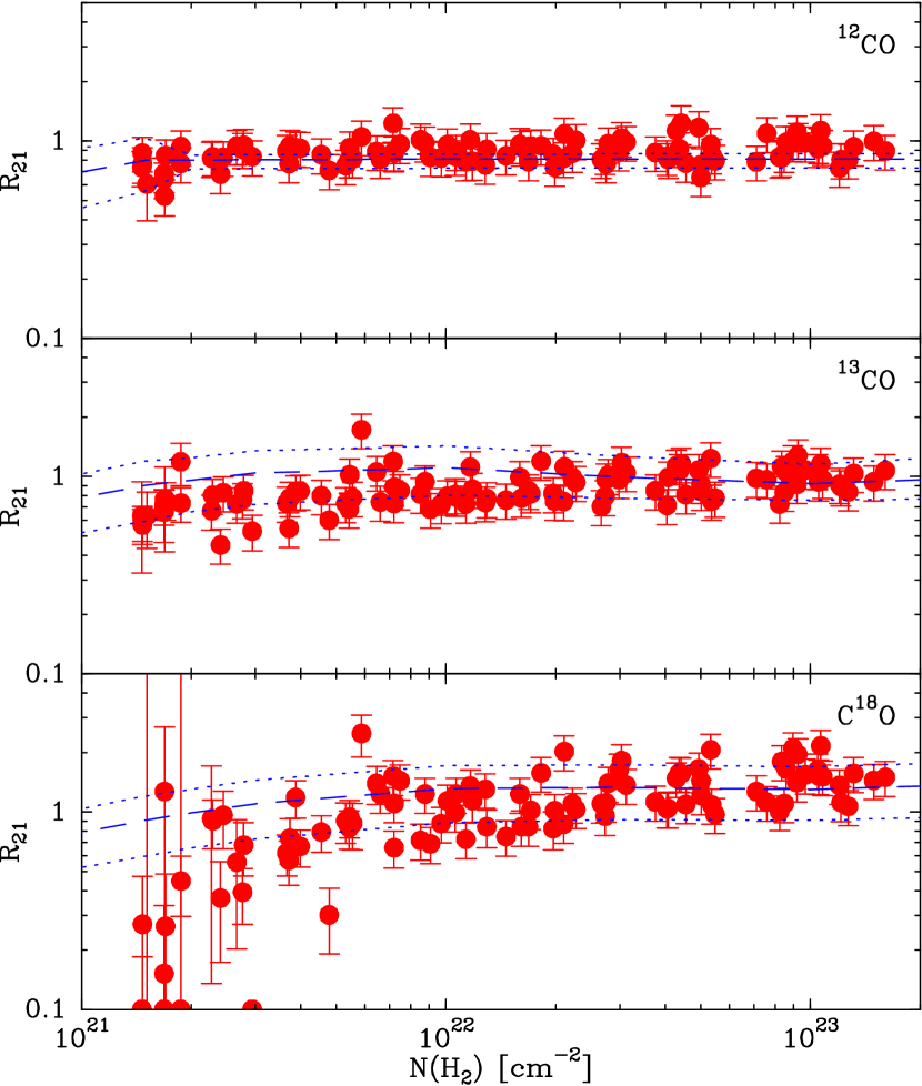
Figure 8: Ratio between $J$=2–1 and $J$=1–0 integrated intensities as a function of H₂ column density for the three CO isotopologs for which both transitions were observed (red circles). The blue dashed line represents the prediction from a radiative transfer model of an isothermal cloud at 11 K. The dotted lines represent similar models for 15 K (higher curve) and 7.5 K (lower curve).

The systematic and relatively simple behavior of the line intensities in Perseus suggest that the emission from the cloud must be controlled by the global properties of its gas, and not by specific details of different parts of the cloud. If this is the case, it should be possible to reproduce the emission behavior using a relatively simple treatment of the gas physical and chemical properties. In this section, we explore this possibility by building a simple cloud model that reproduces simultaneously the main emission properties identified by our Perseus survey. While this model results from a deliberate attempt to reproduce the observations, it should be not be seen as the product of a systematic search for the best possible fit, but as an illustration of how the intensities observed in Perseus can be naturally explained as arising from gas conditions expected to occur in a molecular cloud of its type.

5.1 Physical parameters

Since our data show that the Perseus line intensities depend to first order on the H₂ column density, we modeled the cloud using the H₂ column density as the main physical parameter. All the other gas properties that contribute to the line intensity, such as the temperature, density, velocity dispersion, and molecular abundances were modeled as functions of the cloud H₂ column density using simple parametric expressions. The form of these expressions was determined by fitting the intensity of transitions known to be sensitive to specific physical properties. Table. 3 summarizes our choice for the physical parameters, and Appendix C does the same for the molecular abundances.

To determine the cloud gas temperature profile, we used the 2–1/1–0 intensity ratio of ¹²CO, ¹³CO, and C¹⁸O since these species span a large range of optical depths and are easily thermalized due to their low dipole moment. As Fig. 8 shows, the 2–1/1–0 ratio of the three CO isotopologs is approximately constant over the full range of column densities, suggesting that an isothermal solution may be able to fit the data. Such type of solution would also be in line with the estimated dust temperature, which presents an approximately constant value over the whole cloud (Zari et al., 2016). A natural choice for the model gas temperature is 11 K since it corresponds to the average value determined by Rosolowsky et al. (2008a) using NH₃ observations of almost 200 dense cores. Fig. 8 shows that 11 K indeed provides a reasonable fit to the data (blue dashed lines), and while the fit quality could be slightly improved by adding small ad hoc deviations from isothermality, the constant temperature profile was preferred in the name of simplicity.

A constant temperature solution may at first seem surprising since the cloud outer layers are likely warmer than the interior (Wannier et al., 1983). Detailed modeling of molecular cloud surfaces by Wolfire et al. (2010), however, shows that the CO-emitting gas that we used for the temperature determination is almost insensitive to this outer warming because the same UV photons that are responsible for the warming are also responsible for photodissociating CO (see also Glover & Clark 2012). The net result of this process is that most of the warm outer gas is CO dark, and most of the CO-emitting gas remains at a close-to-constant temperature of 10 K. This effect can be best seen in Figs. 4 and 6 from Wolfire et al. (2010), which show that the gas temperature remains close to 10 K all the way from the cloud interior to an $A_{\mathrm{V}}$ of about 2, which corresponds to the inner edge of the lowest column density bin in our sampling. Only the outer 1 $A_{\mathrm{V}}$ magnitude of the cloud contains CO-emitting gas that is warmer than 10 K, a fact that our modeling cannot test well due to the weak signal of the emission. Any temperature increase in the outer cloud will therefore only affect our modeling of the already poorly constrained outermost bin.

The second cloud parameter that we model is the volume density of the gas. Assigning a single volume density to a given column density represents a very strong simplification since any line of sight through the cloud likely contains densities that vary by more than one order of magnitude. As discussed below, this simplification limits the quality of the fits, but unfortunately is necessary if we are to use a simple radiative transfer model. To determine the best-fit density profile we used a more indirect approach than for the temperature since no molecular line or line ratio is significantly more sensitive to this density than others. After some experimentation, we chose to fit simultaneously the emission from multiple transitions of the traditional dense gas tracers HCN (J=1–0 and 3–2) and CS (J=2–1, 3–2, and 5–4) because they approximately span the range of upper level energies covered by our line survey. The results of this fitting are shown below since they also depend on the abundance profiles discussed in Sect. 5.2. Here we just state that the fit requires a gas volume density that depends on the column density approximately as a power law of the form $N$(H₂)^0.75.

While the above density profile represents our favored choice to fit the observed line emission, it should be considered only as a model parameterization. It represents a not-well-defined line-of-sight average weighted by the emissivity of the different lines, and it likely spans a limited range of values compared with the true range of volume densities in the cloud. This can be seen from the fact that if we were to use a similar relation to determine the spatial extent of the gas in the different density regimes assuming simply that $N({\mathrm{H}}_{2})=n({\mathrm{H}}_{2})\times L$, a steeper density profile would be required to reproduce the observed larger extent of the lower-density gas. Unfortunately, no similar global fit of the emission has been carried on other clouds, so it is not possible to compare our results with previous work. We note however, that a similar (or close to linear) density dependence with column density can be seen in the compilation of numerical simulations presented by Bisbas et al. (2019) (their appendix B).

Table 3: Model physical parameters

Parameter	Value
$T_{\mathrm{K}}$	$11$ K
$n(\mathrm{H}_{2})$	$2\times 10^{4}\;\mathrm{cm}^{-3}\;(N(\mathrm{H}_{2})/10^{22}\;\mathrm{cm}^{-2})^{0.75}$
$\Delta V$	$1\;\mathrm{kms}^{-1}\;(N(\mathrm{H}_{2})/10^{22}\;\mathrm{cm}^{-2})^{0.15}$

The final physical quantity required by our model is the gas velocity dispersion. We parameterized it using the observed linewidth of C¹⁸O(2–1) since this line is optically thin and was observed with relatively high velocity resolution (0.27 km s^-1) due to its higher frequency. The top panel of Fig. 9 shows that the C¹⁸O(2–1) linewidth increases weakly with H₂ column density in a way that we parameterized as $N$(H₂)^0.15 (dashed line). This linewidth increase with column density is likely caused by the star formation activity in the high column density bins. As Fig. 1 shows, these bins are concentrated in the main star-forming regions of the cloud (NGC 1333, B1, and L1448), and many of their CO spectra present wings indicative of outflow contamination. Surveys of both Taurus and Perseus have shown that the linewidth of the C¹⁸O lines tends to be larger in dense cores with stars compared to starless cores (Zhou et al., 1994; Kirk et al., 2007), and the survey of Taurus cores by Onishi et al. (1996) found a systematic increase in the C¹⁸O linewidth with H₂ column density similar to the one found by us in Perseus.

The lower panels of Fig. 9 show that the J=2–1 linewidth of the more abundant isotopologs ¹³CO and ¹²CO is significantly larger than that of C¹⁸O(2–1), by factors of 1.75 and 4, respectively. These larger linewidths most likely result from optical depth broadening (e.g., Hacar et al. 2016), and since the radiative transfer model described below does not reproduce this feature, we incorporated them explicitly into the model when predicting the ¹³CO and ¹²CO emission.

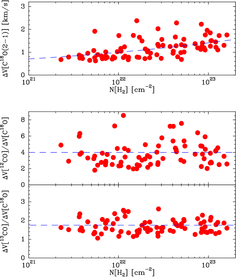
Figure 9: Gas internal motions. Top: C¹⁸O(2–1) FWHM linewidth as a function of H₂ column density derived from Gaussian fits to the spectra (red circles). The dashed line represents an analytic approximation used to model the trend. Bottom: Linewidth ratios of the two main CO isotopologs over C¹⁸O. The dashed lines represent the constant ratios used in the model (4 for ¹²CO and 1.75 for ¹³CO).

5.2 Chemical abundances

Figure 10: Comparison between observations and model results for the family of CO isotopologs. The red symbols represent the observed intensities of the $J$=1–0 line, previously presented in Fig. 4, and the dashed blue lines represent the model results. The sharp drop at low column densities is caused by the photodissociation edge in the abundance profile.

Once the physical properties of the model cloud were fixed, the only parameter left to fit the emission of each species was its abundance profile. We aimed to describe these profiles using a parameterization that is both simple and consistent with our current knowledge of the chemical processes occurring in a molecular cloud like Perseus. After some exploring, we found that reasonable fits can be obtained by using a parameterization containing three terms:

$$X({N(\mathrm{H_{2}}}))=X_{0}\times f_{\mathrm{out}}(N({\mathrm{H_{2}}}))\times f_{\mathrm{in}}(N({\mathrm{H_{2}}})),$$ (1)

where $X_{0}$ represents a constant scaling factor, and $f_{\mathrm{out}}$ and $f_{\mathrm{in}}$ are two normalized factors that represent abundance changes with respect to $X_{0}$ in the outer and inner parts of the cloud (i.e., at low and high H₂ column densities).

Appendix C provides a detailed discussion of the meaning of the different factors and the analytic expressions used in the model. In this section, we summarize the main ideas that are required to understand the model results presented below.

The $f_{\mathrm{out}}$ factor represents any abundance change that takes place in the outer layers of the cloud, likely as a result of their exposure to the external UV radiation field. It is dominated by the contribution of molecular photodissociation in a thin outer layer of a few magnitudes of extinction, a process that has been modeled in great detail by previous chemical work (e.g., Tielens & Hollenbach 1985; van Dishoeck & Black 1988; Le Bourlot et al. 1993; Sternberg & Dalgarno 1995; Visser et al. 2009; Wolfire et al. 2010; Joblin et al. 2018). In our model, a simple photodissociation drop seems enough to fit the observed intensities of most species in the lowest column density bins. For these species, we used an analytic formula based on the realistic PDR models of Röllig et al. (2007). This formula is presented in Appendix C, and has as its only free parameter the location of the sharp edge expressed in units of $A_{\mathrm{V}}$. Changes in this parameter allow the model to adjust for the still poorly characterized value of the UV radiation field in the cloud, which has been previously estimated to have a Draine $\chi$ parameter (Draine, 1978)) between 1-3 (Pineda et al., 2008) or 24 (Navarro-Almaida et al., 2020). It should be noted, however, that the low column-density intensities for most species are too weak to constrain the location of the edge, so most lines were fitted with a fixed value of $A_{\mathrm{V}}=2$ mag (the value derived for CO).

For C₂H and CN, the data show an intensity enhancement in a layer interior to the photodissociation edge, so we complemented the drop term with a more gradual outward abundance enhancement. This term is based on the detailed modeling of the Orion Bar PDR by Cuadrado et al. (2015), who found evidence for an outer abundance increase in the small hydrocarbons driven by gas-phase reactions involving C⁺.

The final factor in our abundance parameterization is $f_{\mathrm{in}}$, which describes possible variations in the cloud interior (i.e., at high $N$(H₂) values). For all species except N₂H⁺, the data require a systematic abundance decrease with $N$(H₂), likely caused by freeze out. This is consistent with previous findings toward starless dense cores in different environments (Caselli et al., 1999; Bergin et al., 2002; Tafalla et al., 2002), and for this reason, we parameterized $f_{\mathrm{in}}$ with an expression used by Tafalla et al. (2002) to describe such systems. This expression has as only free parameter the volume density characteristic of freeze out, which has been adjusted for each molecular species. As with the photodissociation edge, a narrow range of choices (1-$2\times 10^{5}$ cm^-3) is enough to fit all the observations.

For N₂H⁺, the observations require an abundance enhancement toward the cloud interior, in agreement with the theoretical expectation that this species increases its abundance when CO freezes out (Bergin & Langer, 1997; Aikawa et al., 2001). To parameterize this effect, we used a simple expression related to that used for freeze out, and which is further described in Appendix C.

As an additional constraint to the model, we required that the relative abundances of the isotopologs follow the ratios determined for the local ISM by Wilson & Rood (1994). We thus assumed the following isotopic ratios: 77 for ¹²C/¹³C, 560 for ¹⁶O/¹⁸O, 3.2 for ¹⁸O/¹⁷O, and 22 for ³²S/³⁴S.

5.3 Model results

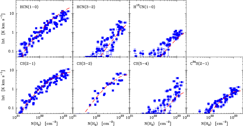
Figure 11: Comparison between observations and model results for HCN (top) and CS (bottom). Each row presents the intensity of the different transitions observed for the species (main and rare isotopologs) as a function of H₂ column density (blue symbols) together with the predictions from the model (dashed red lines). The CS(3–2) dataset has fewer points due to the limited observations carried out in the 2mm-wavelength band. Several H¹³CN(1–0) points can be seen above the plot lower limit at very low column densities. A visual inspection of their spectra suggests that they represent noise or baseline residuals and not true molecular emission.

To predict the emergent line intensities from the cloud model, we used a large velocity gradient (LVG) approximation to the radiative transfer (Castor, 1970; Scoville & Solomon, 1974). This approximation provides a reasonable estimate of the emission given the uncertain geometry of the cloud (White, 1977), and thanks to its speed, allows exploring efficiently a large range of input cloud parameters. Our LVG code is based on that presented by Bieging & Tafalla (1993), and was complemented with molecular data compiled by the Leiden Atomic and Molecular Database (LAMDA), which is continually updated with the most recent literature values (Schöier et al., 2005; van der Tak et al., 2020). In this section, we present the results of modeling several representative species that illustrate the different emission behaviors identified in the cloud. Modeling results for the rest of the species and a table summarizing the abundance parameters derived from the fits are presented in Appendix D.

Fig. 10 shows the model results for the $J$=1–0 transition of the CO isotopologs (dashed blue lines). Similar results were obtained for the $J$=2–1 transitions, as can be inferred from the fit to the 2–1/1–0 ratios shown in Fig. 8. The $X_{0}$ value of the different CO isotopologs was set by fixing the value of C¹⁸O to the determination by Frerking et al. (1982) ($=1.7\times 10^{-7}$) and using the already-mentioned isotopic ratios from Wilson & Rood (1994). In addition, the model assumed a photodissociation edge of $A_{\mathrm{V}}$ = 2 mag and a freeze-out critical density of $10^{5}$ cm^-3 for all CO isotopologs.

As can be seen from Fig. 10, the cloud model, although not perfect, fits reasonably well the emission. This is remarkable given the simplicity of the model and the small number of free parameters used to adjust the fit since once the cloud physical parameters have been fixed, only three free parameters ($X_{0}$, the $A_{\mathrm{V}}$ value of the photodissociation edge, and the freeze-out density) are left to reproduce the intensity of the four CO isotopologs over two orders of magnitude in H₂ column density. According to the model, the ¹²CO lines are optically thick and thermalized everywhere inside the photodissociation edge, and the slight intensity increase with the H₂ column density arises from the similar increase in the linewidth. The ¹³CO line, on the other hand, only becomes optically thick at H₂ column densities higher than $2\times 10^{22}$ cm^-2. As expected, the C¹⁸O and C¹⁷O lines are optically thin everywhere inside the cloud.

A number of shortcomings in the model can be attributed to our simplified treatment of the abundance of the different CO isotopologs. Our model assumes that they are scaled versions of each other, while in reality the ¹³CO abundance is expected to increase with respect to ¹²CO near the cloud edge due to isotopic fractionation, and the C¹⁸O and C¹⁷O abundances are expected to decrease in the same region due to isotope-selective photodissociation (Bally & Langer, 1982; van Dishoeck & Black, 1988). These two effects would likely enhance the ¹³CO intensity and decrease the C¹⁸O and C¹⁷O intensities in the vicinity of the photodissociation edge, improving the fit results.

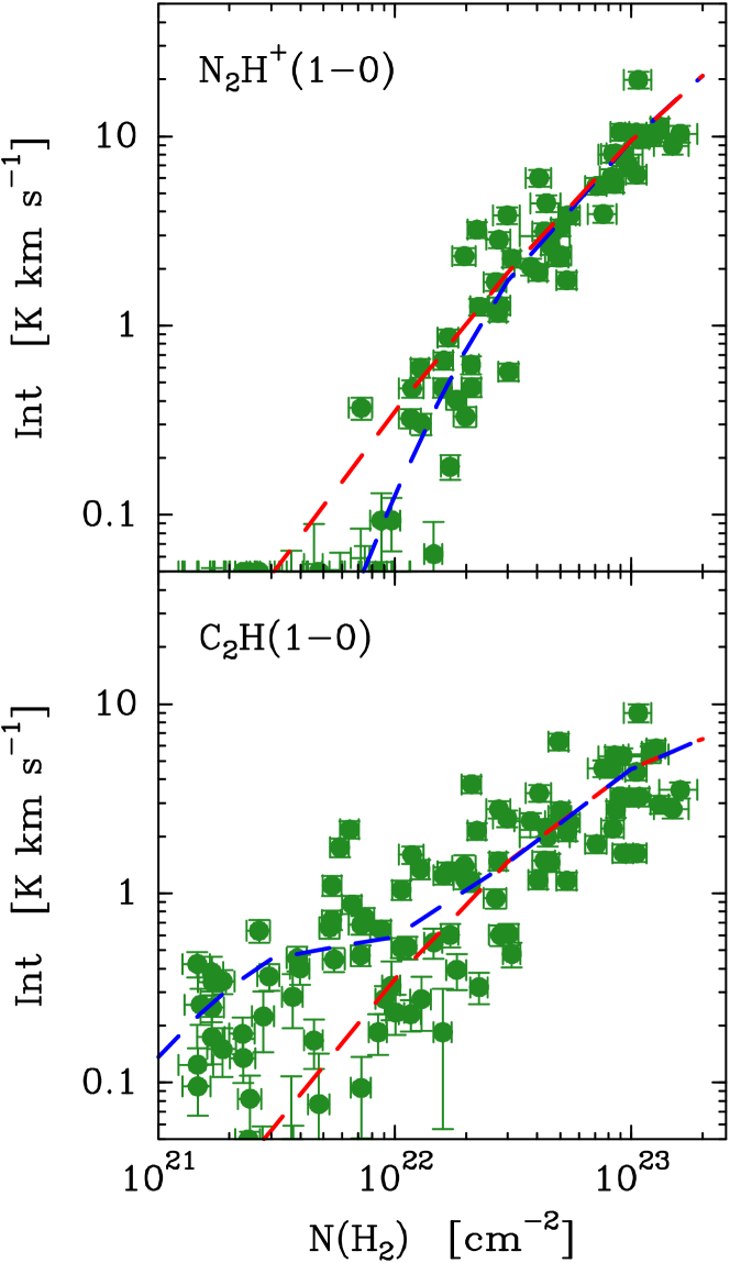
Figure 12: Comparison between observations and model results for two species that require special abundance profiles: N₂H⁺ (top) and C₂H (bottom). In both panels, the green symbols represent the observed intensity, previously shown in Fig. 5. In the N₂H⁺ panel, the dashed red line represents a constant abundance model that fits the intensity at high column densities. The blue dashed line represents the best-fit model, and includes an internal abundance enhancement. In the C₂H panel, the dashed red line represents a model with no external enhancement, while the blue line represents the externally enhanced best-fit model.

To explore the ability of the cloud model to fit the intensity of the traditional dense gas tracers, we focus here on HCN and CS, which are the most widely used members of this family. Appendix D presents the results for the remaining members. For HCN and CS, our observations provided intensities for all sample positions of the transitions in the 1 and 3mm wavelength bands, and for CS, a limited number of positions were also observed in the 2mm wavelength band. In addition, the 3mm transitions of H¹³CN and C³⁴S were also detected and included in the model.

Fig. 11 compares all the available HCN and CS data (blue symbols) with the predictions from our cloud model (dashed red lines). The model assumes the same abundance factor $X_{0}$ ($=3\times 10^{-9}$) and photodissociation edge ($=2$ mag) for both species, while the freeze-out critical density is $2\times 10^{5}$ cm^-3 for HCN and $10^{5}$ cm^-3 for CS. As with the CO isotopologs, a simple three-parameter model approximately fits simultaneously all the observed line intensities over the full range of cloud column densities.

While the model intensities remain within the scatter of the data points, and are therefore consistent with the observations, Fig. 11 shows that the model does not provide the best possible fit. The HCN model slightly overestimates the $J$=1–0 intensity of the main isotopolog while it underestimates the intensity of H¹³CN. For CS, the model reproduces well the $J$=2–1 transition of both the main and rare isotopologs together with the 3–2 intensity, but it is close to the lower boundary of the $J$=5–4 data points. Both deviations, and similar ones found in the modeling of HNC and HCO⁺ (Appendix D), likely result from the use of a single density value to represent the complex cloud structure along any given line of sight. In a real cloud, the density along any line of sight likely increases toward the interior. As a result, an optically thick line like HCN(1–0) will sample lower densities than an optically thin line like H¹³CN(1–0). This effect will decrease the HCN(1–0) intensity and increase the H¹³CN(1–0) intensity compared to our model, in agreement with the observations. Also, a high critical density line, like CS(5–4), will be sensitive to the highest density gas along the line of sight, an effect that is again missed by our single-density assumption. As mentioned above, fixing these fitting imperfections would require having a realistic description of the multiple density regimes present along any line of sight. Lacking such a description, we consider that our single-density model provides a reasonably good fit to the observed intensities.

As a final illustration of our modeling, we present in Fig. 12 the solutions for N₂H⁺ and C₂H, the two species that, together with CN, require special abundance profiles. The top panel of the figure compares the N₂H⁺ data with the prediction from two abundance models. The dashed red line corresponds to a constant-abundance model set to fit the observed intensities at high $N$(H₂). As can be seen, the model significantly overestimates the intensities in the outer cloud, indicating the need of an abundance drop at low $N$(H₂). The second model (dashed blue line) corresponds to the profile described in Appendix C, and has a significant abundance drop at low H₂ column densities, as expected from the destruction of N₂H⁺ by CO when the latter species is abundant in the gas phase (Bergin & Langer, 1997; Aikawa et al., 2001). This modified model reproduces the emission both at high and low H₂ column densities, and is therefore in better agreement with the observations. It should be noted, however, that our data sampling in the transitional region ($N(\mathrm{H}_{2})\approx 10^{22}$ cm^-2) is not fine enough to constrain well the abundance drop, and that the drop could be sharper than suggested by the model. Additional observations of the N₂H⁺ emission in this transitional region and at lower column densities are needed to fully characterize the distribution of this unique dense gas tracer through the entire cloud.

The bottom panel of Fig. 12 shows the model results for the C₂H(1–0) line. Again, the panel compares two abundance models with the survey data. The dashed red line represents a standard abundance model that has both outer photodissociation and inner freeze-out contributions. This model fits the emission in the inner cloud, but fails to reproduce the observations at very low column densities. The dashed blue line corresponds to an abundance profile that has an outer enhancement next to the photodissociation edge, and that is inspired by the PDR model of the C₂H abundance from Cuadrado et al. (2015) (see Appendix C for a full description). As can be seen, this modified model reproduces better the emission enhancement near the outer edge of the cloud in addition to the cloud interior. A similar model, but with a smaller outer enhancement, is also needed to fit the CN emission, as shown in Appendix D.

We summarize our modeling results by saying that the Perseus data suggest that the shape of the abundance profile of any species is mostly controlled by how the species reacts to two agents: (i) the UV ISRF at low column densities and (ii) dust collisions at high column densities. All our survey species except N₂H⁺, C₂H, and CN behave passively with respect to these agents, in the sense that they are photodissociated by the UV radiation and they freeze out onto the dust grains. As a result, the abundance of these species decreases both toward the outer edge and inside of the cloud in a manner illustrated by the top panel of Fig. 18.

The three exceptions we found to the above abundance pattern result from some type of active reaction to either the UV radiation or to the collisions with the dust. In the case of C₂H and CN, these species are enhanced near the cloud edge as a result of the UV ISRF, and in the case of N₂H⁺, this molecule thrives when CO starts to freeze out. These two behaviors are illustrated in the middle and bottom panels of Fig. 18. When taken into account, the complete set of observed lines in Perseus can be reproduced with a relatively simple model.

The fact that a simple model like the one presented here can reproduce the line intensities of so many species and transitions suggests that the main properties of the line emission in the Perseus cloud are controlled by a small number of processes that can be simulated with a few model parameters. Whether this behavior is peculiar to Perseus or common to other clouds requires further investigation, and will be explored in future work.

6 Discussion

6.1 Origin of the intensity dependence with column density

Since our cloud model reproduces the main features of the Perseus emission, we can use it to investigate the origin of the different correlations between intensity and H₂ column density found for different species. Of particular interest is the comparison between the correlation of the CO isotopologs, which present a rather flat dependence with $N$(H₂), and the correlation of the traditional dense gas tracers HCN and CS, which approximately follow a linear dependence with $N$(H₂).

To investigate the origin of these different correlations, we look separately at the two factors that contribute to the intensity in the solution of the equation of radiative transfer: $J(T_{\mathrm{ex}})-J(T_{\mathrm{bg}})$ and $(1-e^{-\tau})$, which we will refer to as the “excitation” factor and the “optical depth” factor, respectively. In Fig. 13 we present their value as a function of $N$(H₂) for the 3mm lines of the main CO, HCN, and CS isotopologs (solid lines) and the rare isotopologs C¹⁸O, H¹³CN, and C³⁴S (dashed lines).

As Fig. 13 shows, the excitation factor for both the main and rare CO isotopologs (top panel, solid and dashed red lines) has an approximately constant value close to the gas kinetic temperature minus the background temperature, as expected for species that are thermalized over most of the cloud. The optical depth factor, on the other hand, is different for the main and rare CO isotopologs (bottom panel, red lines). For the main isotopolog, the optical depth factor has a close-to-constant value of 1 over most of the cloud due to the extremely high optical depth of the emission. For the less abundant C¹⁸O, the optical depth factor reflects closely the C¹⁸O column density, which is not linear with $N$(H₂), but curves downward at high values due to the increasing effect of freeze out. When the excitation and optical depth factors are multiplied to obtain the intensity, the result is an approximately constant function for CO and a slightly curved intensity law for C¹⁸O, as observed in the data.

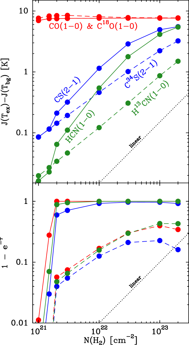
Figure 13: Model results for the two factors of the radiative transfer solution: excitation term (top) and optical depth term (bottom). The solid lines represent the results for the main isotopologs of CO (red), HCN (green), and CS (blue). The dashed lines represent equivalent results for the rare species (C¹⁸O, H¹³CN, and C³⁴S).

For the HCN and CS isotopologs, the excitation factor differs sharply from that of CO. As can be seen from the green and blue lines in the top panel of Fig. 13, while the excitation factor of CO is flat, that of HCN and CS increases rapidly with $N$(H₂). This increase is a consequence of the HCN and CS lines being significantly subthermal, and therefore having an excitation that increases rapidly as the volume density increases with $N$(H₂). For the main HCN and CS isotopologs (solid lines), the excitation has an additional contribution from photon trapping due to the high optical depth of the lines, and this enhances their factor over that of the rare isotopologs, for which trapping is insignificant (dashed lines). Independently of this extra contribution, the excitation factor of all the HCN and CS isotopologs increases by about two orders of magnitude over the H₂ column density range of the cloud.

In contrast with the excitation factor, the optical depth factor of HCN and CS behaves like that of CO (bottom panel). For the main isotopologs, the factor has an almost constant value of one inside the photodissociation edge, while for the less abundant isotopologs, it presents a less-than-linear increase with $N$(H₂) due to the effect of freeze out. This similarity with CO is not surprising since all the species have similar abundance profiles, and the main isotopologs are very optically thick while the rare ones are thin.

The similar behavior of the optical depth factors of CO and the traditional dense gas tracers indicates that the different dependence of the intensity of HCN-CS and CO with $N$(H₂) in the cloud interior arises mainly from a difference in the excitation of the molecules. For the CO isotopologs, the combination of flat excitation factors due to thermalization with flat or not too steep optical depth factors results in relatively flat intensity correlations with $N$(H₂). For HCN and CS, the steep excitation factors resulting from subthermal excitation dominate the dependence of the emergent intensities and are ultimately responsible for the strong correlation of the intensities with $N$(H₂).

To understand why the intensity of the main and rare isotopologs of HCN and CS present similar dependence with $N$(H₂), we need to consider now the combined effects of excitation and optical depth. As seen in the top panel of Fig. 13, the main isotopologs (solid lines) have significantly steeper excitation factors than the rare isotopologs (dashed lines) due to the additional contribution from photon trapping. These factors have slopes that, although not constant, are close to linear, as can be seen from a comparison with the dotted line shown in the panels. When these factors are multiplied by the almost constant optical depth factors, the resulting intensities retain the close-to-linear slope.

The rare isotopologs, on the other hand, present slightly flatter excitation factors due to the missing trapping contribution. When these factors are multiplied by the optical depth factors, which have a non-negligible slope over most of the $N$(H₂) range, the resulting emergent intensity approaches the linear slope of the thick main isotopologs. It seems therefore that the similar behavior of the thin and thick traditional dense gas tracers as a function of H₂ column density results from the approximate compensation of their different excitation and optical depth factors. While somewhat fortuitous, this behavior seems to be very robust since it is displayed by most observed species in multiple transitions, and ultimately gives rise to the systematic quasi-linear emission pattern found by most dense gas tracers in our survey.

6.2 What the traditional dense gas tracers trace

The almost linear dependence with H₂ column density of the emission from species like HCN and CS forces us to reevaluate the traditional distinction between dense gas tracers and column density tracers used to classify molecules. The correlations found in Perseus imply that, strictly speaking, only N₂H⁺ deserves the term dense gas tracer since it is the only species truly selective of the dense gas: its emission remains undetected below around $10^{22}$ cm^-2 (corresponding in our model to a density of $2\times 10^{4}$ cm^-3), and then rises nonlinearly when $N$(H₂) exceeds the threshold. This unique behavior of N₂H⁺ has been previously seen at core scales (Caselli et al., 1999; Bergin et al., 2002; Tafalla et al., 2002) and at cloud scales (Kauffmann et al., 2017; Pety et al., 2017), and results from the sensitivity of N₂H⁺ to the presence of CO in the gas phase. Although no other molecule in our survey presents a similar behavior, it is likely that NH₃ may do so since NH₃ shares with N₂H⁺ a resilience to freeze out in addition to being a late-time chemical species (Suzuki et al., 1992; Tafalla et al., 2002). Indeed, observations of N₂H⁺ and NH₃ toward Perseus dense cores have found a strong correlation between the emission of these two species (Johnstone et al., 2010; Hacar et al., 2017). Extending our Perseus observations to include the cm-wavelength NH₃ lines would be highly desirable to test this prediction.

Although HCN, CS, and the other traditional dense gas tracers do not display the selectivity to the dense gas of N₂H⁺, they are still sensitive to the cloud dense material in an indirect way. This is so because their emission follows the column density, which we have seen is itself an indirect indicator of the gas volume density. These tracers, therefore, are brighter toward the higher column density gas, which results from the presence of dense gas along the line of sight. For this reason, tracers like HCN and CS are still useful to identify the densest parts of molecular clouds in spatially resolved maps, as proven by numerous previous studies (e.g., Plume et al. 1997; Beuther et al. 2002; Wu et al. 2010).

The lack of selectivity to the dense gas of HCN, CS, and similar tracers is a more serious problem in unresolved observations of molecular clouds, as those commonly used in extragalactic work. In this type of work, interpreting the emission from the different tracers is not straightforward since this emission represents a weighted average to which all the density regimes in the cloud contribute. The relevant parameter in this case is the product of the column density probability distribution function (PDF) times the line intensity as a function of column density. As we have seen, the Perseus data show that for HCN, CS, and other tracers, the intensity is approximately linear with $N$(H₂), while the column density PDF depends much more steeply on the parameter, as $N$(H₂)^-3 (Zari et al., 2016). As a result, the integrated emission will be dominated by the contribution from the lowest column density positions, whose nonlinear overabundance more than compensates for the approximately linear decrease in their intensity.

A similar dominant contribution of the low-density gas in the cloud-integrated emission from the traditional dense gas tracers has also been found by several studies, and likely represents a general trend among molecular clouds (Kauffmann et al., 2017; Pety et al., 2017; Watanabe et al., 2017; Shimajiri et al., 2017; Nishimura et al., 2017; Evans II et al., 2020). This finding should be not surprising if in most clouds, as in Perseus, the PDF has a very steep negative dependence with $N$(H₂) (Lombardi et al., 2015), while the line intensities depend almost linearly with $N$(H₂) (e.g., Pety et al. 2017). These two behaviors naturally combine to make the contribution of the low column density positions increasingly more important in the cloud-integrated intensity.

Even if the integrated emission of the traditional dense gas tracers is dominated by the low-density gas, it still has a relevant physical interpretation. We have seen that in Perseus the emission follows quasi-linearly the column density in the region above the photodissociation threshold. As a result, the cloud-wide integrated intensity, which is obtained integrating the product of the PDR times the intensity as a function of the column density, will be proportional to the mass of the cloud above the photodissociation threshold. Since our models indicate a threshold of about $A_{\mathrm{V}}=2$ mag for most species, the cloud-integrated intensity of these tracers will be proportional to the mass of the gas above two magnitudes of $A_{\mathrm{V}}$.

While no other cloud has been characterized using the sampling method we used for Perseus, we have seen that an approximately linear dependence of the intensity with the column density is a likely feature of several other clouds (Sect. 4.5). If this is so in general, the same relation between cloud-integrated intensity and mass above the photodissociation threshold of a cloud will apply. Such a possibility, which clearly requires further investigation, is of interest for extragalactic work, where there is evidence for a linear correlation between the emission of tracers such as HCN(1–0) and the rate of star formation (Gao & Solomon, 2004; Kennicutt & Evans, 2012; Usero et al., 2015; Jiménez-Donaire et al., 2019). Interpreting the observed line intensities as estimates of the cloud mass inside a certain column density threshold could potentially help explain the origin of the correlation.

Given the above, it is worth noting that Lada et al. (2010) have found that for local clouds (including Perseus), the mass above a column density threshold of $A_{\mathrm{V}}\approx 7.3$ mag ($A_{\mathrm{K}}\approx 0.8$ mag) is linearly proportional to the star-formation rate of the cloud. This 7.3 mag threshold is significantly higher than the photodissociation threshold we found in Perseus, so the mass derived using the Lada et al. (2010) threshold is different from (and much smaller than) the mass inferred from the HCN(1–0) intensity. It is therefore unclear whether the Lada et al. (2010) relation can help connect the cloud-integrated HCN(1–0) intensity with the star-formation rate as found by extragalactic observations. One possibility is that the masses set by the 2 and 7.3 mag thresholds are linearly correlated, something that is possible given the quasi-universal power-law nature of the column density PDFs Lombardi et al. (2015).

The above speculations clearly show that an observational effort is needed to characterize the emission from multiple clouds and test whether our Perseus results reflect a more general trend. For such an effort, the stratified random sampling method presented here appears to be an ideal tool.

7 Conclusions

We used stratified random sampling to select 100 target positions that represent the different regimes of the H₂ column density in the Perseus molecular cloud. We observed these positions with the IRAM 30m telescope covering the 3mm-wavelength band and selected parts of the 2mm and 1mm bands. We studied the correlation of the observed line intensities with the H₂ column density, and we developed a simple cloud model to reproduce the main features of the emission. The main conclusions from this work are the following.

1. A comparison of our sampling results for ¹²CO(1–0) and ¹³CO(1–0) with the mapping data from the COMPLETE project shows that stratified random sampling can be used to estimate the mean intensity and the intensity dispersion of these two lines as a function of column density within a factor of 1.5 or better.

2. The intensity of the molecular lines in Perseus strongly correlates with the H₂ column density over the two orders of magnitude that this quantity spans through the cloud. The lines of the CO isotopologs and the traditional dense gas tracers (CS, HCN, HCO⁺, etc.) present a level of dispersion in the intensity-$N$(H₂) relation of only about 0.2 dex. This tight correlation between line intensities and H₂ column density supports the use of column density as a proxy of the intensity for the stratified random sampling, as initially motivated by principal component analysis (Ungerechts et al., 1997; Gratier et al., 2017).

3. The intensity of the CO isotopologs increases slower than linearly with $N$(H₂), while the intensity of most dense gas tracers increases approximately linear with $N$(H₂).

4. Several dense gas tracers present significant deviations from a linear dependence with $N$(H₂). The largest deviation is that of N₂H⁺(1–0), which presents a very rapid transition from undetected to relatively bright near $N$(H₂) = $10^{22}$ cm^-2. C₂H(1–0) and (to smaller extent) CN(1–0) present significant enhancements in their intensity at low column densities (¡ $10^{22}$ cm^-2).

5. The main emission trends identified in the Perseus data are similar to those recently reported from multiline mapping of entire clouds (e.g., Kauffmann et al. 2017; Pety et al. 2017; Watanabe et al. 2017). This similarity suggests that the sampling technique can truly characterize efficiently the emission from a cloud. It also points to a general behavior of the emission in clouds that span a relatively large range of star-formation conditions.

6. A simple cloud model can reproduce the main emission features of Perseus. For most species, the model requires a molecular abundance that has a sharp drop at low column densities (likely due to photodissociation) and a more gradual decrease at high column densities (likely caused by freeze out). The only species that require different abundance distributions are N₂H⁺, which is enhanced when CO freezes out, and C₂H and CN, which are enhanced by the external UV field. The different abundance behaviors of these species are consistent with our current understanding of molecular cloud chemistry.

7. Our cloud model suggests that the flat dependence with $N$(H₂) of the CO isotopologs results from a combination of optical depth effects and molecular freeze out under thermalized conditions. The quasi-linear behavior of most traditional dense gas tracers and their isotopologs results from the increase in excitation with column density combined with molecular freeze out toward the densest gas. A lucky compensation between excitation in the optically thick species and column density effects in the rare isotopologs is responsible for their similar behavior with $N$(H₂).

8. The cloud-integrated emission of the traditional dense gas tracers is dominated by the contribution from the lowest column density positions because their nonlinear overabundance (described by the PDF) more than compensates for the approximately linear decrease in their intensity. The quasi-linear dependence of their intensity with $N$(H₂) makes the integrated intensity of these tracers approximately proportional to the mass of the gas interior to the photodissociation edge. This property may help provide a physical meaning to the integrated intensity of these tracers in unresolved observations.

Appendix A Sample positions and 3mm line intensities

Table 4 presents the coordinates, column density estimates, and 3mm line intensities for the 100 sample positions used in the Perseus survey. A full version of the table is available on-line.

Table 4: Sample positions and line intensities.

Position	RA(J2000)	Dec(J2000)	$N$(H2)	12CO(1–0)	13CO(1–0)	C18O(1–0)	C17O(1–0)	HCN(1–0)	CS(2–1)	HNC(1–0)	HCO+(1–0)
	(h  m  s)	(°  ′  ″)	(cm-2)	(K km s-1)	(K km s-1)	(K km s-1)	(K km s-1)	(K km s-1)	(K km s-1)	(K km s-1)	(K km s-1)
PERS-10_01	03 29 04.7	+31 14 44.8	$1.0\;(0.1)\times 10^{23}$	118 (12)	30 (3)	4.6 (0.5)	1.3 (0.1)	12 (1)	9.4 (0.9)	9.5 (1.0)	10.0 (1.0)
PERS-10_02	03 29 09.4	+31 13 35.6	$1.6\;(0.3)\times 10^{23}$	82 (8)	25 (3)	3.6 (0.4)	1.1 (0.1)	13 (1)	11.4 (1.1)	9.2 (0.9)	7.8 (0.8)
PERS-10_03	03 29 16.0	+31 12 29.6	$1.1\;(0.1)\times 10^{23}$	73 (7)	22 (2)	3.2 (0.3)	0.88 (0.09)	4.9 (0.5)	4.4 (0.4)	4.1 (0.4)	3.4 (0.3)
PERS-10_04	03 33 16.7	+31 07 18.0	$1.2\;(0.1)\times 10^{23}$	51 (5)	21 (2)	5.6 (0.6)	2.0 (0.2)	4.7 (0.5)	4.9 (0.5)	4.7 (0.5)	2.6 (0.3)
PERS-10_05	03 25 36.0	+30 45 57.2	$1.2\;(0.2)\times 10^{23}$	49 (5)	19 (2)	3.2 (0.3)	0.92 (0.1)	11 (1)	6.2 (0.6)	9.7 (1.0)	7.8 (0.8)
PERS-10_06	03 33 15.8	+31 07 03.9	$1.3\;(0.1)\times 10^{23}$	48 (5)	20 (2)	5.5 (0.6)	2.2 (0.2)	4.0 (.4)	3.8 (0.4)	3.7 (0.4)	1.7 (0.2)
PERS-10_07	03 29 02.2	+31 15 32.1	$1.1\;(0.1)\times 10^{23}$	105 (10)	36 (4)	5.2 (0.5)	1.5 (0.2)	11 (1)	9.7 (1.0)	9.3 (0.9)	14.2 (1.4)
PERS-10_08	03 29 10.8	+31 14 29.3	$1.1\;(0.1)\times 10^{23}$	73 (7)	23 (2)	3.2 (0.3)	0.75 (0.08)	8.1 (0.8)	7.3 (0.7)	6.8 (0.7)	5.7 (0.6)
PERS-10_09	03 29 09.7	+31 14 40.3	$1.3\;(0.1)\times 10^{23}$	78 (8)	23 (2)	2.9 (0.3)	0.86 (0.09)	9.0 (0.9)	7.1 (0.7)	8.1 (0.8)	6.2 (0.6)
PERS-10_10	03 29 13.5	+31 13 16.8	$1.5\;(0.3)\times 10^{23}$	72 (7)	24 (2)	3.7 (0.4)	1.2 (0.1)	5.5 (0.6)	5.4 (0.5)	4.5 (0.4)	3.9 (0.4)

Appendix B Stacked spectra

Figs. 14, 15, and 16 present stacked spectra for the 3 mm-wavelength transitions discussed in Sect. 4.2. The stacking was done by averaging the ten spectra of each column density bin after having shifted the lines to zero velocity using a Gaussian fit to the ¹³CO(1–0) line. To ease inter-comparing the spectra, each plot uses the same intensity scale (in units of $T_{\mathrm{mb}}$). Most spectra have been scaled by factors of $1.6^{n}$, where $n$ depends on the bin number, to approximately compensate for the change in H₂ column density between the bins.

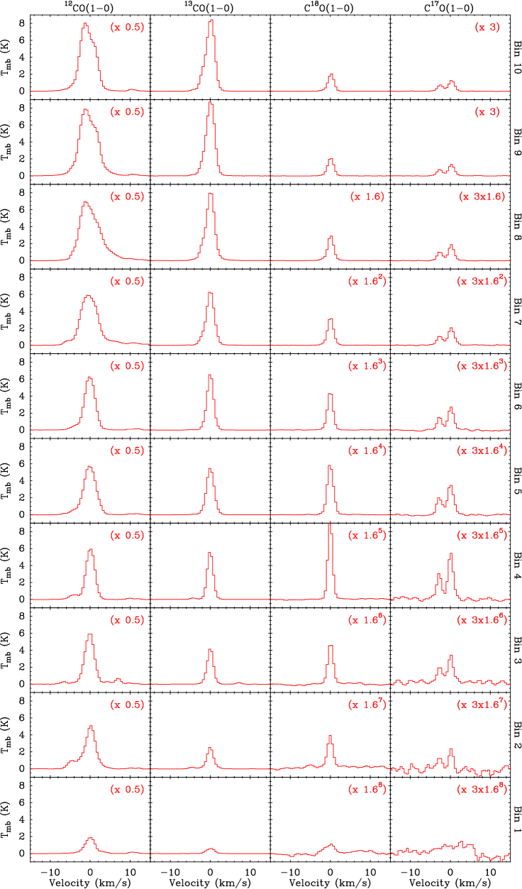
Figure 14: Stacked spectra of the $J$=1–0 transition for different CO isotopologs Each spectrum represents the average of the ten spectra taken in the column-density bin indicated in the right label. The mean column density of these bins decreases downward by factors of 1.6, and the spectra have been scaled up by different factors to approximately maintain the same physical size.

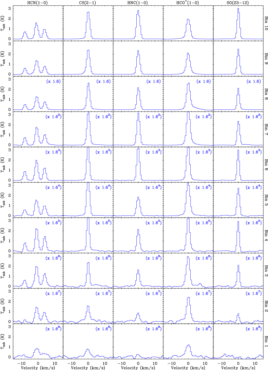
Figure 15: Same as Fig. 14 but for the traditional dense gas tracers: HCN(1–0), CS(2–1), HNC(1–0), HCO⁺(1–0), and SO(23–12).

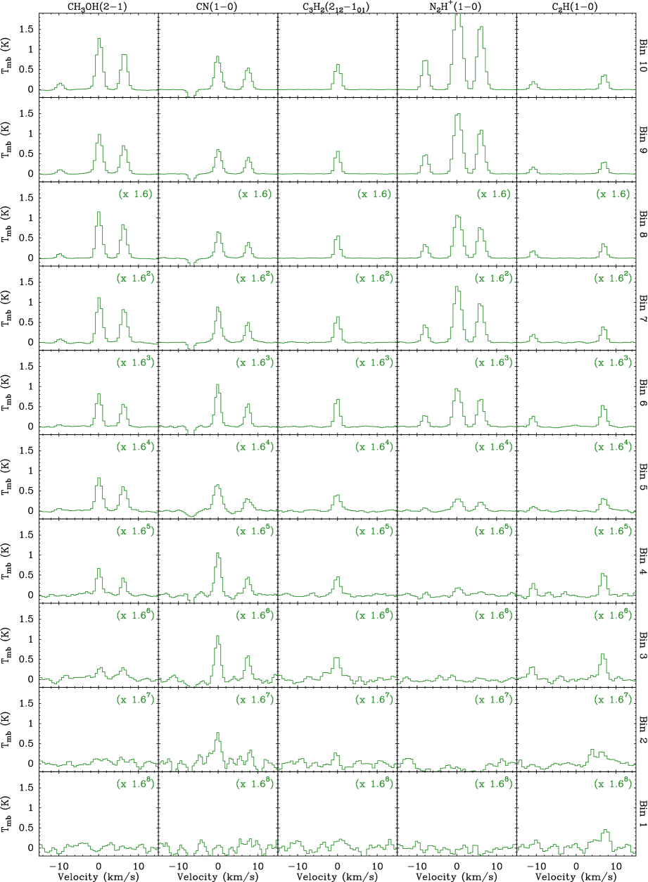
Figure 16: Same as Fig. 14 but for the additional gas tracers: CH₃OH(2–1), CN(1–0), C₃H₂(2₁₂–1₀₁), N₂H⁺(1–0), and C₂H(1–0). For CN(1–0) and C₂H(1–0), only a subset of the hyperfine components is shown due to the limited velocity window. The negative CN(1–0) feature near -7 km s^-1 is an artifact from the frequency switching observing mode.

Appendix C Modeling abundance profiles

As mentioned in Sect. 5.2, our cloud model aims to provide a description of the abundance profiles that is both simple and consistent with the chemical processes known to occur in a cloud. To this end, we found convenient to write the abundance profile of each species (with respect to H₂) as the product of three factors,

$$X({N(\mathrm{H_{2}})})=X_{0}\times f_{\mathrm{out}}(N({\mathrm{H_{2}}}))\times f_{\mathrm{in}}(N({\mathrm{H_{2}}})),$$

where $X_{0}$ is a constant scaling, $f_{\mathrm{out}}$ represents a departure from constant near the outer edge of the cloud, likely caused by the UV photons from the interstellar radiation field, and $f_{\mathrm{in}}$ represents a departure from constant at high column densities, likely related to molecular freeze out.

For all species but C₂H and CN, the $f_{\mathrm{out}}$ factor needed to fit the data represents a sharp abundance drop that we associate with the photodissociation of the molecules by the external UV radiation field. Although the detailed shape of this drop is not very critical for our modeling due to the lack of column-density resolution near the cloud edge, we used a realistic profile based on the photon dominated region (PDR) models of Röllig et al. (2007). As a representative profile, we selected the CO abundance curve estimated by these authors in their F1 model ($n$(H₂) = $5\times 10^{3}$ cm^-3, and $\chi=10$). This model has a Draine $\chi$ parameter (Draine 1978) that is intermediate between the values favored by Pineda et al. (2008) from their fit of the Perseus CO lines ($\chi=1$-3) and the recent determination for B1 by Navarro-Almaida et al. (2020) using a a model of the dust temperature ($\chi=24$). We fitted this profile using the following analytic expression

$$f_{\mathrm{out}}(N({\mathrm{H_{2}}}))=\cases{[}e^{(A_{\mathrm{V}}-A_{0})}]^{6}&{\mathrm{if}}\leavevmode\nobreak\ \leavevmode\nobreak\ \leavevmode\nobreak\ A_{\mathrm{V}}\leq A_{0}\\ 1{\mathrm{if}}\leavevmode\nobreak\ \leavevmode\nobreak\ \leavevmode\nobreak\ A_{\mathrm{V}}>A_{0},{}$$

where $A_{\mathrm{V}}$ is the H₂ column density expressed in units of visual extinction ($N$(H₂) = $9.35\times 10^{20}A_{\mathrm{V}}$ cm^-2, Bohlin et al. 1978). $A_{0}$ is a free parameter that describes the location of the photodissociation edge also in units of visual extinction and allows for changes in the value of $\chi$ with respect to the original model. Fig. 17 compares a set of abundance values extracted from Fig. 4b in Röllig et al. (2007) (red circles) with our analytic expression for a choice of $A_{0}=1.5$ mag (blue line). As shown below in Table 5, the $A_{0}$ values needed to fit the Perseus data range between 1 and 2 mag, in good agreement with the theoretical expectation from the PDR model. It should be noted, however, that for most species, our observations cannot constrain the exact location of the photodissociation edge due to the limited signal to noise ratio of the intensities at low column densities and the coarseness of the column density bins. For these species, we used a single value of 2 mag based on the results from the CO data. This choice provides a reasonable match to the data, but it should not be considered as a well-defined best fit.

Since the C₂H and CN intensities require a significant abundance enhancement in the vicinity of the photodissociation edge, we multiplied the $f_{\mathrm{out}}$ factor of these species by the additional term

$$f^{\prime}_{\mathrm{out}}(N({\mathrm{H_{2}}}))=1+\alpha\;e^{-A_{\mathrm{V}}/3},$$

where the free parameter $\alpha$ describes the magnitude of the outer abundance enhancement. This additional factor was inspired by the detailed modeling of the C₂H abundance in the Orion Bar PDR by Cuadrado et al. (2015), who found that the species undergoes an abundance enhancement of several orders of magnitude in the vicinity of the cloud edge (their Fig. 17).

The last factor in our abundance parameterization is $f_{\mathrm{in}}$, which describes deviations from a constant value in the cloud interior. For all species but N₂H⁺, the data requires a significant abundance drop at high column densities that is likely caused by freeze out onto the dust grains. Following previous freeze-out modeling by Tafalla et al. (2002), we described this abundance drop with the simple analytic expression

$$f_{\mathrm{in}}(N({\mathrm{H_{2}}}))=e^{-n(\mathrm{H}_{2})/n_{\mathrm{fr}}},$$

where $n(\mathrm{H_{2}})$ is the gas density (related to $N$(H₂) by the cloud parameterization described in Sect. 5.1), and $n_{\mathrm{fr}}$ is a free parameter that describes the characteristic freeze-out density of the species. As shown in Table 5, all species in the sample can be fitted with $n_{\mathrm{fr}}$ values in the range $(1-2)\times 10^{5}$ cm^-3, characteristic of molecular freeze out.

For the freeze-out resistant N₂H⁺ molecule, the above expression was substituted by

$$f^{\prime}_{\mathrm{in}}(N({\mathrm{H}_{2}}))=1-e^{-(n(\mathrm{H}_{2})/n_{\mathrm{fr}})^{2}},$$

which represents an abundance enhancement, and where $n_{\mathrm{fr}}$ is again a free parameter that describes the characteristic density at which the N₂H⁺ enhancement occurs.

Fig. 18 presents the three types of abundance profiles generated using our three-factor parameterization that were needed to fit the variety of intensity behaviors identified in our Perseus survey. The top panel presents the abundance profile used to fit all species excluding N₂H⁺, C₂H, and CN. This profile is characterized by a sharp photodissociation edge at low column densities, a close-to-constant abundance value at intermediate column densities, and a gradual abundance drop due to freeze out at high column densities. We refer to this profile as the “standard” one. The middle panel shows the abundance profile needed to fit the N₂H⁺ emission. It presents an opposite behavior to the standard profile at high column densities: an initial rapid abundance increase followed by a close-to-constant value. Finally, the bottom panel presents the abundance profile used to fit the C₂H emission (a similar one was used for CN). This profile presents a significant enhancement at low column densities followed by an external photodissociation edge.

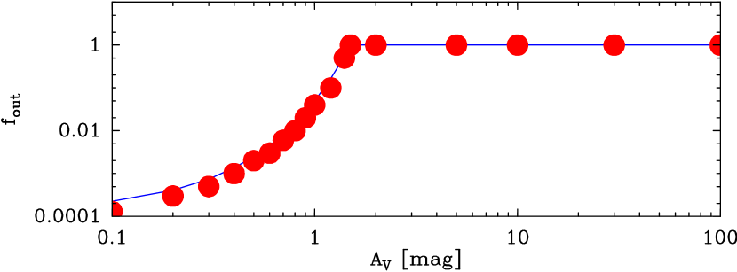
Figure 17: Abundance factor used to model the cloud photodissociation edge. The red symbols represent values of the CO abundance predicted by the F1 PDR model of Röllig et al. (2007) and extracted from their Fig. 4b. The solid blue line is the analytic expression described in the text for a choice of $A_{0}=1.5$ mag.

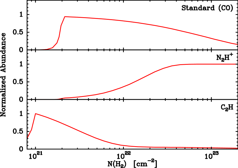
Figure 18: Three types of abundance profiles generated by a simple model and used to fit the emission from different species in Perseus. Top panel: Standard abundance profile consisting of an outer photodissociation edge and an inner freeze-out drop. It was used to fit most molecular data and is illustrated here with CO. Middle panel: Profile with an inner enhancement required to fit the N₂H⁺ data. Bottom panel: Profile with an outer abundance enhancement required to fit the C₂H and CN data (illustrated here with C₂H).

Appendix D Fitting results for remaining species

In Sect. 5.3 we presented radiative transfer results for a representative group of molecular species that cover the different emission behaviors found in Perseus: the family of CO isotopologs, CS and HCN (as examples of traditional dense gas tracers with standard abundance profile), and N₂H⁺ and C₂H, two species with inner and outer abundance enhanced profiles, respectively. In this Appendix we present the model results for the remaining species of the survey.

As mentioned in Sect. 5.3, our model aims to fit simultaneously for each species all the transitions of the main and rare isotopologs detected in the 1mm, 2mm, and 3mm wavelength windows covered by the survey. We assume that the abundances of the different isotopologs are related by the ratios estimated by Wilson & Rood (1994) in the solar vicinity.

Fig. 19 presents the fit results for the tracers not presented in Sect. 5.3: the traditional dense gas tracers HNC, HCO⁺, and SO (blue symbols), and the additional tracers CH₃OH, CN, and C₃H₂ (green symbols). For each species, all observed transitions and isotopologs are presented in the same row, except for CN and C₃H₂, for which only one transition was detected, and which are presented together in the bottom row for space reasons.

As can be seen in the figure, the model predictions (dashed lines) generally lie within the cloud of observed data points, indicating that the model provides a reasonable fit to the observations. Some deviations from the expected best fit are seen in species where the lines span a large range of optical depths, such as HNC and HCO⁺. These deviations are similar to those found when fitting the CS and HCN data, in the sense that our model has difficulty reproducing simultaneously the $J$=1–0 lines of the main and rare isotopologs because our solution slightly overestimates the thick main line while it underestimates the thin isotopolog line. As discussed in Sect. 5.3, this fitting problem likely results from the use of a single volume density to characterize the physical conditions along any given line of sight, a choice that ignores the complex density structure present in the real cloud. Apart from this limitation, the model seems to work reasonably well considering its small number of free parameters, the large number of molecular species considered, and the large dynamic range span by the intensities. For these reasons we believe that the model captures the main features of the physical and chemical structure of the Perseus molecular cloud.

Table 5 summarizes the abundance best-fit parameters used to model the emission from each survey species. It also provides references for the collision rate coefficients used to model the excitation. As mentioned in Sect. 5.3, these coefficients, together with any additional molecular parameters, were input into the radiative transfer code using the files provided by the LAMDA database (Schöier et al. 2005; van der Tak et al. 2020).

A significant result from Table 5 is that the abundance values derived for Perseus match closely abundance estimates made for other star-forming regions. As mentioned before, the $A_{0}$ values of the photodissociation edge and the characteristic freeze-out density $n_{\mathrm{fr}}$ agree with previous observations and chemical model predictions for typical clouds (e.g., Bergin & Langer 1997; Caselli et al. 1999; Bergin et al. 2002; Tafalla et al. 2002; Röllig et al. 2007; Pineda et al. 2008). In addition, the $X_{0}$ values in Table 5 for all species with the exception of C₃H₂ agree within a factor of three with the geometrical mean of the undepleted abundances in the Taurus-Auriga L1498 and L1517B dense cores estimated by Tafalla et al. (2006) (the difference for C₃H₂ is a factor of 6). Considering that these two estimates used very different radiative transfer assumptions and even different collision rates, the agreement is notable. It suggests once again that the gas properties derived from our Perseus analysis are likely representative of the gas properties in other star-forming regions.

Table 5: Best-fit abundance parameters and collision-rate coefficients

Species	$X_{0}$	$A_{0}$	$\alpha$	$n_{\mathrm{fr}}$	Coll. Coeff.
		(mag)		(cm-3)	Reference
CO	$9.5\;10^{-5}$	2	0	$10^{5}$	1
HCN	$3\;10^{-9}$	2	0	$2\;10^{5}$	2
CS	$3\;10^{-9}$	2	0	$10^{5}$	3
HNC	$10^{-9}$	2	0	$2\;10^{5}$	4
HCO+	$1.5\;10^{-9}$	2	0	$2\;10^{5}$	5
SO	$10^{-9}$	2	0	$2\;10^{5}$	6
CH3OH	$1.5\;10^{-9}$	2	0	$2\;10^{5}$	7
CN	$1.5\;10^{-9}$	1	5	$2\;10^{5}$	8
C3H2	$2\;10^{-10}$	2	0	$2\;10^{5}$	9
N2H+	$1.5\;10^{-10}$	2	0	$3\;10^{4}$	10
C2H	$2\;10^{-9}$	1	20	$2\;10^{5}$	11

(1) Yang et al. (2010); (2) Hernández Vera et al. (2017); (3) Lique et al. (2006); (4) Dumouchel et al. (2010); (5) Flower (1999); (6) Lique et al. (2007); (7) Rabli & Flower (2010); (8) Kalugina & Lique (2015); (9) Chandra & Kegel (2000); (10) Daniel et al. (2005); (11) Spielfiedel et al. (2012).

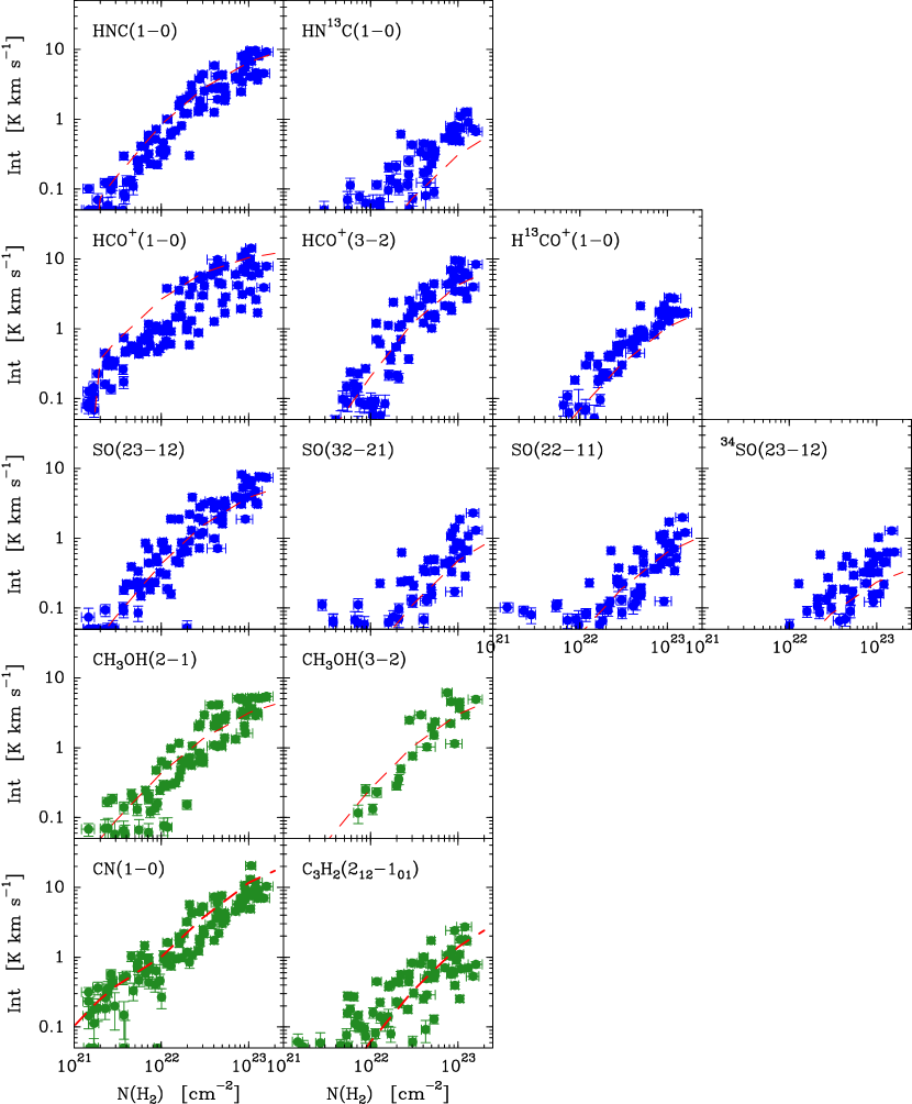
Figure 19: Comparison between observations and model results for the species not presented in the main text. The data points represent the observations (traditional dense gas tracers in blue and additional tracers in green), and the red dashed lines represent the model results. Each panel row contains all observed transitions and isotopologs of any given molecular species, except for the last row that shows together the only observed lines of CN and C₃H₂. Several SO and C₃H₂ points can be seen above the plot lower limit at very low column densities. A visual inspection of their spectra suggests that they represent noise or baseline residuals, and not true molecular emission.