3D mapping of the Crab Nebula with SITELLE. I. Deconvolution and kinematic reconstruction

Abstract

We present a hyperspectral cube of the Crab Nebula obtained with the imaging Fourier transform spectrometer SITELLE on the Canada-France-Hawaii telescope. We describe our techniques used to deconvolve the 310 000 individual spectra ($R=9\,600$) containing H$\alpha$, [N ii] $\lambda\lambda$6548, 6583, and [S ii] $\lambda\lambda$6716, 6731 emission lines and create a detailed three-dimensional reconstruction of the supernova remnant assuming uniform global expansion. We find that the general boundaries of the 3D volume occupied by the Crab are not strictly ellipsoidal as commonly assumed, and instead appear to follow a “heart-shaped” distribution that is symmetrical about the plane of the pulsar wind torus. Conspicuous restrictions in the bulk distribution of gas consistent with constrained expansion coincide with positions of the dark bays and east-west band of He-rich filaments, which may be associated with interaction with a pre-existing circumstellar disk. The distribution of filaments follows an intricate honeycomb-like arrangement with straight and rounded boundaries at large and small scales that are anti-correlated with distance from the center of expansion. The distribution is not unlike the large-scale rings observed in supernova remnants 3C 58 and Cassiopeia A, where it has been attributed to turbulent mixing processes that encouraged outwardly expanding plumes of radioactive ⁵⁶Ni-rich ejecta. These characteristics reflect critical details of the original supernova of 1054 CE and its progenitor star, and may favour a low-energy explosion of an iron-core progenitor. We demonstrate that our main findings are robust despite regions of non-homologous expansion driven by acceleration of material by the pulsar wind nebula.

1 Introduction

Young supernova (SN) remnants ($<3000$ yr) in the Milky Way and Magellanic Clouds provide rare opportunities to probe the explosion mechanisms and progenitor systems of SNe with observations capable of producing three dimensional reconstructions. Their proximity (from a few to less than a hundred kpc) and high expansion velocity (a few thousand km s^-1) allow not only to disentangle the different Doppler components with relatively modest spectral resolutions, but also to determine the tangential velocity of their filaments using images obtained decades apart (or sometimes a few years apart using the Hubble Space Telescope; HST). Asymmetries in chemical or ionization structure, expansion velocity or density can then be probed with much greater precision than what is possible for unresolved extragalactic objects (Milisavljevic & Fesen, 2017). Such reconstructions, made for SNRs including Cassiopeia A (Cas A) (DeLaney et al., 2010; Milisavljevic & Fesen, 2013; Alarie et al., 2014; Milisavljevic & Fesen, 2015; Grefenstette et al., 2017), 1E 0102.2-7219 (Vogt & Dopita, 2010; Vogt et al., 2018), and N132D (Law et al., 2020), are critical for establishing strong empirical links between SNe and SNRs that can be compared to state-of-the-art simulations evolving from core collapse to remnant (Orlando et al., 2015, 2016; Orlando et al., 2020; Ono et al., 2020).

Among the most studied yet still enigmatic remnants deserving of 3D reconstruction is the Crab Nebula (SN 1054, NGC 1952). Despite decades of investigation, the progenitor star’s initial mass and the properties governing the SN explosion remain uncertain (Davidson & Fesen, 1985; Hester, 2008). The total mass of its ejecta (2-5 M_⊙; Fesen et al. 1997) is much less than the plausible mass of the progenitor (8-13 M_⊙; Nomoto 1987), and although SN 1054 was more luminous than a normal Type II SN ($-18$ mag vs. $-15.6$ mag; Clark & Stephenson 1977), its kinetic energy ($\approx 7\times 10^{49}$ erg) is surprisingly low compared to the canonical $\sim 10^{51}$ erg. The standard explanation is that most of the mass and 90% of the kinetic energy of SN 1054 reside in an invisible freely expanding envelope of cold and neutral ejecta traveling $\sim 5000$  km s^-1 far outside the Crab (Chevalier, 1977). However, this theorized outer envelope has never been robustly detected to remarkably low upper limits (Fesen et al., 1997; Lundqvist & Tziamtzis, 2012). A weak C IV $\lambda$1550 absorption feature observed in a far-ultraviolet HST spectrum of the Crab pulsar is suggestive of an ionized outer envelope (Sollerman et al., 2000; Hester, 2008), but only extending out to $\sim 2500$ km s^-1 and tracing a relatively small amount of material ($\sim 0.3$ M_⊙).

Models and observations generally support a low energy SN origin potentially associated with an O-Ne-Mg core that collapses and explodes as electron-capture supernova (ECSN) (Nomoto et al., 1982; Hillebrandt, 1982; Kitaura et al., 2006). However, such explosions are generally faint ($M_{V}$ $>-15$ mag) and thus inconsistent with the brightness of SN 1054 estimated from historical records. Fesen et al. (1997) and Chugai & Utrobin (2000) suggested that SN 1054 was a low energy SN with additional luminosity provided by circumstellar interaction. Smith (2013) supports this view and identified potential Crab-like analogs in many recent Type IIn events. Tominaga et al. (2013) found that the high peak luminosity could instead be related to the large extent of the progenitor star and not necessarily associated with strong circumstellar interaction. Gessner & Janka (2018) questioned the appropriateness of an ECSN origin for the Crab, as their simulations found that hydrodynamic neutron star kicks associated with O-Ne-Mg core progenitors are much below the $\sim 160$ km s^-1 measured for the Crab pulsar (Kaplan et al., 2008). Yang & Chevalier (2015) found the Crab’s overall properties to be consistent with expectations from a pulsar wind nebula evolving inside a freely expanding low energy supernova.

There have been multiple attempts at mapping the three dimensional structure of the Crab. However, the large angular size of the Crab ($\sim$6′) and complexity of its numerous overlapping filamentary structures presents many challenges. Lawrence et al. (1995) created three-dimensional spatial models of the line-emitting [O III] $\lambda\lambda$4959, 5007 gas in the Crab with Fabry-Perot imaging spectroscopy. Čadež et al. (2004) created a 3D representation using long slit spectroscopy at low and high resolution configurations rotated at a series of position angles. Charlebois et al. (2010) used the imaging Fourier transform spectrometer SpIOMM to create a 3D view of the Crab and emission line ratios of the filaments. Black & Fesen (2015) mapped the Crab’s northern ejecta jet with moderate resolution [O III] line emission spectra. Generally, these investigations have highlighted the north-south bipolar asymmetry in the abundance, geometry, and velocity distribution of the bright filaments. A band of helium-rich material runs in the east-west direction (Uomoto & MacAlpine, 1987a), which is associated with pinched velocities (MacAlpine et al., 1989a), potentially associated with constrained expansion due to interaction with a circumstellar disk left behind from pre-SN mass loss (Fesen et al., 1992). To date there does not exist a complete mapping of individual emission lines throughout the remnant sensitive to faint emission on fine scales.

In this paper we introduce a hyperspectral cube of the Crab obtained with the imaging Fourier transform spectrometer SITELLE (Drissen et al., 2019). SITELLE has a field of view of 11′$\times$ 11′, high sensitivity down to 350 nm, and is especially powerful for observing emission line sources above a low continuum background (Bennett, 2000; Maillard et al., 2013). Together, these characteristics make SITELLE uniquely suited to meet the challenges of observing the Crab.

In this paper we describe preliminary SITELLE observations and associated analysis of the Crab obtained in a passband covering 647-685 nm with spectral resolution 9 600. These data are the highest resolution ever obtained with SITELLE on an astrophysical target and a spectacular opportunity to demonstrate the full potential of this new technology. We also describe the techniques used to deconvolve the spectra and produce a 3D reconstruction of the supernova remnant. A more detailed analysis of these data in combination with planned complementary observations at other wavelengths will follow in a subsequent paper.

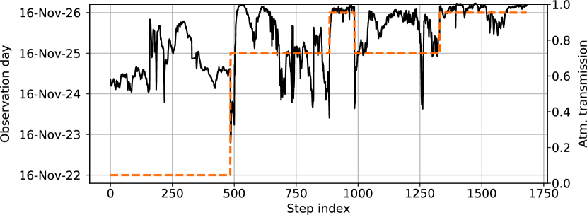
Figure 1: Atmospheric transmission as a function of the step index. The date when each part of the cube was obtained is shown as an orange dotted line.

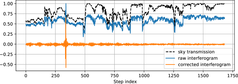
Figure 2: Interferogram of the M1 pulsar before and after the correction for the sky transmission and the varying background (resp. blue and orange line). Atmospheric transmission is reported in dotted black. The large oscillation seen at step $\sim 325$ corresponds to the Zero path difference of the interferometer, and is characteristic of a continuum source, while the low-amplitude beating patterns observed along the interferogram are caused by the multiple emission lines of the nebula included within the $1.6^{\prime\prime}$ radius of the aperture.

2 Data

2.1 SITELLE data

The data were obtained using the SITELLE instrument mounted to Canada-France-Hawaii telescope (CFHT) during the course of an engineering run spanning the nights of November 22, 25 and 26, 2016. SITELLE combines a 2D imaging detector with a Michelson interferometer. Two complementary interferometric data cubes are obtained by recording images, on two 2k$\times$2k CCD detectors, at different positions of the moving mirror inside the Michelson. Fourier transforms are then used to convert these cubes into a single spectral data cube. Spectral resolution is set by the maximum path difference between the two arms of the interferometer, reached by displacing its moving mirror through a series of steps of several hundred nanometers each. The spectral range is selected by using interference filters; SITELLE covers the 350 - 850 nm range with a series of 8 filters, tailored to specific needs. Spatial sampling is $0.32^{\prime\prime}$ per pixel, leading to a field of view of $11^{\prime}\times 11^{\prime}$ and over 4 million spectra.

Our raw data for the Crab consist in an interferometric cube of 1682 steps (with a step size of 2843 nm) with an exposure time of 5.3 s per step (followed by an overhead of 3.8 s for CCD readout and concurrent mirror movement and stabilization), leading to an integration time of 2.48 hours over a 4.25 hours total data aquisition time. The median seeing, measured on the image obtained from the combination of all detrended and aligned interferometric images, was 1.17$\pm 0.04$ ″. This engineering data was aimed at testing SITELLE’s high resolution capabilities with a target resolution of 10 000 in the SN3 filter (647 - 685 nm passband: H$\alpha$, [N ii]$\lambda\lambda$6548,6584, [S ii]$\lambda\lambda$6717,6731). It was obtained under extremely varying atmospheric conditions (see Figure 1). Some data obtained on November 25 (around steps 900 - 1000) were deemed to be of too poor quality and were therefore taken again at the end of the following night.

We thus have been able to test the stability of the instrument in terms of absolute positioning of the moving mirror and the impact of the observed modulation efficiency loss at high optical path difference (OPD) (Baril et al., 2016).

These data were reduced with the pipeline reduction software ORBS (Martin et al., 2012; Martin, 2015) without any special treatment with respect to the rest of the data obtained during the same run. As an example of the quality of the reduction, we present in Figure 2 the raw interferogram of the pulsar, obtained with an aperture of $1.6^{\prime\prime}$ radius, before and after the correction for the sky transmission. Any error on this correction on the interferograms can significantly impact the quality of the calculated spectrum and especially its instrumental line shape (ILS) (Martin & Drissen, 2016).

We have measured the effective resolution by fitting a model on a spectrum of the sky (dominated by OH lines in this spectral range) integrated over a small region of the cube (a circular aperture with a 100 pixels radius) with the analysis software ORCS (Martin et al., 2015). In order to take into account the modulation efficiency loss at high OPD, which may broaden the observed ILS, we have modelized the ILS as the convolution of a sinc (the natural ILS of a Fourier transformed spectrum) with a Gaussian (resulting from the broadening of the observed sky lines by the modulation efficiency loss) and used the sincgauss model described in Martin et al. (2016) (see Figure 3). The measured full-width at half maximum of the sky lines was 1.718$\pm 0.05$ 11 which leads to a resolving power $R=8870\pm 20$ @ H$\alpha$ (Martin et al., 2016). From the parameters of the cube, the theoretical resolution which we should have been measured at the same position is 9640. We can conclude that the effect of the modulation efficiency loss at high OPD is at most of the order of 10 % at a resolution of 9640.

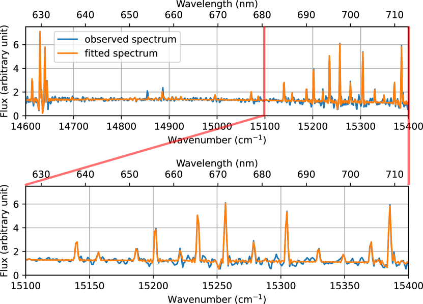
Figure 3: Sky spectrum used to measure the effective resolution ($R=8870\pm 20$) (blue line) along with the fitted model (orange line). The bottom panel shows an enlarged portion of the top panel around H$\alpha$ (15237 cm^-1)

3 Mapping the Crab Nebula in H$\alpha$, [N II] and [S II]

The Crab Nebula is long known to display a very complex filamentary structure that remains interpreted as the result of Rayleigh-Taylor instabilities at the interface of the synchrotron nebula and the thermal ejecta (Hester et al., 1996; Hester, 2008). This filamentary structure, ionized by the shock of the expanding synchrotron nebula, shows’s particularly strong emission in H$\alpha$, [N ii] and [S ii]. Multiple components of filamentary emission are visible along any line of sight with velocities ranging from -1500 to 1500 km s^-1 (see Figure 4) that must be separated in order to compute the correct mapping of the flux and velocity of the observed emission lines. The emission covers a circular surface of $\sim$6 ′ in diameter, which spans approximately one million of the four million spectra contained in the data cube.

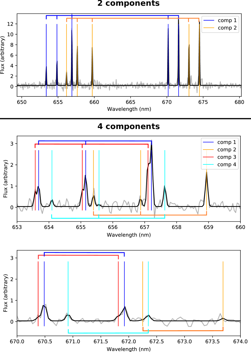
Figure 4: Two examples of spectra containing multiple components and their fit. 2 components panel: A spectrum with 2 non-overlapping components, obtained near the center of the nebula. 4 components panel: A spectrum with 4 overlapping components obtained in a complex filamentary region of the nebula. The plot is split in two parts to help distinguish all 4 components. Note that if only 4 of the components have been found by the algorithm, additional dim components may exist. This example demonstrates at the same time the quality and the limitations of our algorithm.

Inspired by the algorithms developed by Čadež et al. (2004) and Charlebois et al. (2010) on similar data sets, we have written an algorithm to automate detection and fitting of overlapping emission components observed in the spectra. This algorithm analyses each spectrum individually in 3 steps (see Figure 5):

1. evaluation of the probability, as a score, of having one component at a given velocity;

2. enumeration of all the individual velocity components along the line of sight;

3. fit of the spectrum with a model combining all the velocity components at the same time.

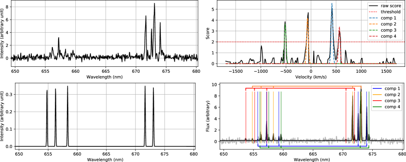
Figure 5: The fitting process. Top-left: Example of a raw spectrum extracted from a complex filamentary region of the nebula containing at least 4 components. Bottom-left: Example of a 5 emission-lines comb-like spectrum which would be convolved with the analyzed spectrum. In fact, the spectrum is convolved with the individual lines of the comb. All lines of the comb have the same intensity. The apparent difference comes from the function sampling. Top-right: Mitigated correlation score obtained after the first step of the analysis (black) with the 4 fitted components detected at the second step. The detection threshold used for the enumeration of the brightest components of the score (see section 3.2) is shown in dotted red. Bottom-right: Fit realized on the spectrum shown in the top-left panel; the positions of the 5 fitted emission-lines are shown for each of the 4 fitted components.

3.1 Step 1: computation of the score

The first step is based on the convolution of the analyzed spectrum $S(\lambda)$ with a comb-like spectrum $K(v,\lambda)$ made of a subset of the emitting lines of each component: H$\alpha$, the [N ii] doublet and the [S ii] doublet (see bottom-left panel of Figure 5). All lines of the comb have the same amplitude. The calculated score $C(v)$ is simply:

$$C(v)=\int S(\lambda)K(v,\lambda)\text{d}\lambda\;.$$ (1)

$C(v)$ is maximum when the position of the modeled emission-lines of $K(v,\lambda)$ coincides with the position of the emission-lines of the spectrum.

Ideally, if the explored velocity range is not too large and no line of the comb is matched with another emission-line, each velocity component of the spectrum will produce one peak with an approximately Gaussian shape. The centroid of the peak gives the component velocity and its amplitude scales with the integral of the flux in the lines present in $K$.

However, the biggest challenge with this approach appears when the comb and the analyzed spectrum contains multiple lines within the range of velocity scanned. For example, one line of the comb (e.g., H$\alpha$) may coincide with the position of a neighbouring line at a different velocity (e.g., [N ii]). In this case, even with only one component along the line of sight, $C(v)$ will show multiple peaks; the highest being the real one because it reflects the velocity at which the largest number of lines are coincident. With multiple components however, if one component is much brighter than the others, the secondary peaks in $C(v)$ created by the brightest component may be even higher than the primary peak of the second components, in which case the correct enumeration of the components is compromised.

Figure 6 reproduces this issue by showing a synthetic spectrum made of two velocity components, one being 5 times brighter than the other. The comb used for the analysis contains 5 emission lines (H$\alpha$, [N ii], [S ii]) and is shown in the bottom-left quadrant of Figure 5.

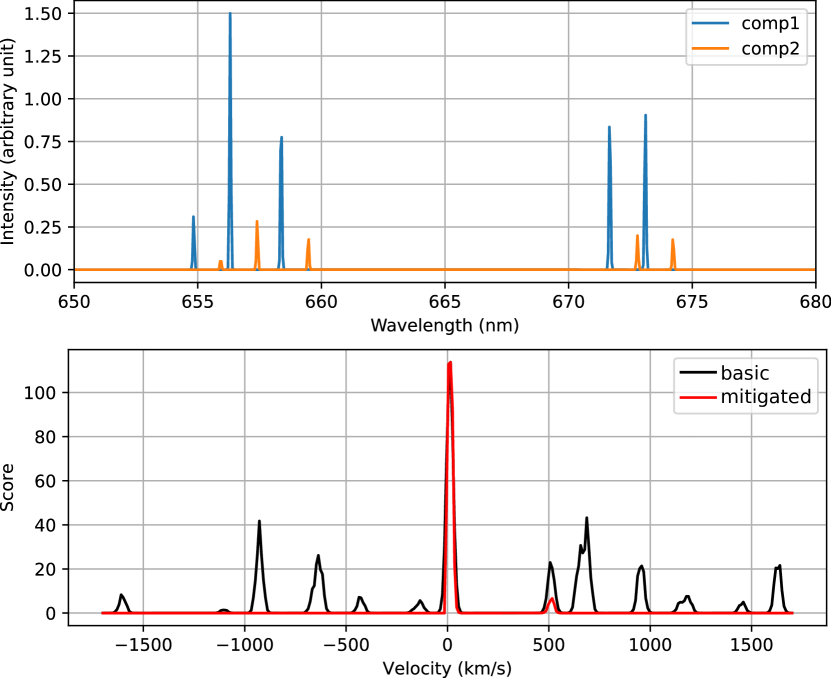
Figure 6: Top: Two-components noiseless model spectrum. Bottom: Basic and mitigated scores computed from the top-panel spectrum. The numerous lines appearing in the basic score (black line) do not reflect real components or noise. Instead, they correspond to velocities where some lines of the comb coincide with another emission line (e.g., where the H$\alpha$ line of the comb coincides, at a given velocity, with an [N ii] line of the spectrum). Applying physical constraints when computing a mitigated score (in red) reduces these aliases, which permits the detection of dimmer velocity components. The addition of noise only contributes small amplitude peaks that are discarded (see top-right panel of Figure 5).

Using equation 1 without any special treatment leads to a score $C(v)$ with multiple false peaks (black line) where the peak related to the dimmest component cannot be retrieved.

We mitigate complicating factors with use of equation 1 by adding a number of physically-based conditions that must be respected in order to get a non-zero value of $C(v)$. One is to force the presence of all the lines by computing independent scores for each line and compute the product of their probability. Let $K_{i}(v,\lambda)$ be the kernel for the line $i$, $i\in\{\textup{H$\alpha$},$ $[\textup{N\,{ii}}]\lambda 6548,$ $[\textup{N\,{ii}}]\lambda 6548,$ $[\textup{N\,{ii}}]\lambda 6583,$ $[\textup{S\,{ii}}]\lambda 6716,$ $[\textup{S\,{ii}}]\lambda 6731\}$. If we want all 5 lines to be present in order to have a non-zero score we would rewrite equation 1 as

$$C_{i}(v)=\int S(\lambda)K_{i}(v,\lambda)\text{d}\lambda\;,$$ (2)

$$C(v)=\Pi_{i}\;C_{i}(v)\;.$$ (3)

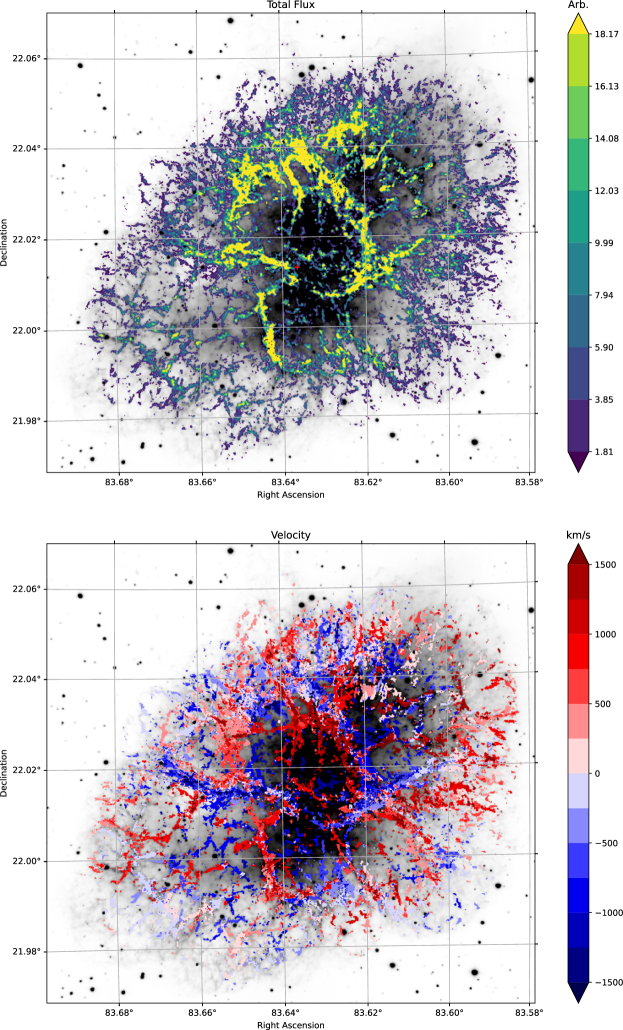
Figure 7: Integral of the emission in all five emission lines (top) and velocity (bottom) maps obtained. When components are overlapping, only the front component is displayed. The color mapping has been discretized for the sake of clarity, but it does not reflect the actual precision of the values. The red cross indicates the center of expansion computed by Kaplan et al. (2008). The velocity uncertainty is shown in Figure 14. The background is the integral of the flux measured (emission lines + continuum) in the whole filter.

However, all 5 lines are not always detectable. Sometimes only the $[\textup{S\,{ii}}]$ or $[\textup{N\,{ii}}]+{\textup{H$\alpha$}}$ lines are visible. Thus we further separate these two groups and put additional physics-based conditions to finally write the mitigated version of the score:

$$C_{[\textup{N\,{ii}}]}=\sqrt{C_{[\textup{N\,{ii}}]\lambda 6548}\times C_{[\textup{N\,{ii}}]\lambda 6583}}\;,$$ (4)

$$C_{[\textup{S\,{ii}}]}=\sqrt{C_{[\textup{S\,{ii}}]\lambda 6716}\times C_{[\textup{S\,{ii}}]\lambda 6731}}\;,$$ (5)

$$C(v)=C_{\textup{H$\alpha$}}\times C_{[\textup{N\,{ii}}]}+C_{[\textup{S\,{ii}}]}\;;$$ (6)

with the following additional conditions that constrain the [S ii] and [N ii] line ratios to be realistic enough,

$$C_{[\textup{N\,{ii}}]}=0\text{ if }C_{[\textup{N\,{ii}}]\lambda 6583}<C_{[\textup{N\,{ii}}]\lambda 6548}\;,$$ (7)

$$C_{[\textup{N\,{ii}}]}=0\text{ if }C_{[\textup{N\,{ii}}]\lambda 6548}<0.14\times C_{[\textup{N\,{ii}}]\lambda 6584}\;,$$ (8)

$$C_{[\textup{S\,{ii}}]}=0\text{ if }C_{[\textup{S\,{ii}}]\lambda 6716}<0.14\times C_{[\textup{S\,{ii}}]\lambda 6731}\;,$$ (9)

$$C_{[\textup{S\,{ii}}]}=0\text{ if }C_{[\textup{S\,{ii}}]\lambda 6731}<0.14\times C_{[\textup{S\,{ii}}]\lambda 6716}\;.$$ (10)

The value of 0.14 ($\simeq 1/7$) has been manually optimized to help reject obviously wrong scores while keeping lower SNR components. This value is necessarily kept lower than the theoretical ratios of [S ii] lines (between 0.5 and 1.5) and [N ii] lines (2.94 in the low-density regime) (Osterbrock & Ferland, 2006) to take into account noise associated with the measured flux.

The results of this mitigated score is drawn on Figure 6 with a red line. The real peaks are both present and all the false peaks have been removed. A more realistic example of this score is also shown in the top-right quadrant of Figure 5, where the false peaks, if not completely removed, have been attenuated enough so that the 4 brightest components are clearly visible.

3.2 Step 2: enumeration of the brightest components

Once the score is obtained, we must go through a peak detection process to enumerate the brightest components and evaluate their velocity, which is done by measuring the centroid of each detected peak. As the components may have similar velocities, their peaks may overlap, which complicates the detection.

We have used an iterative detection procedure not unlike the CLEAN algorithm (Högbom, 1974). At each iteration, only the brightest peak is detected, fitted and removed before moving on to the next iteration until no peaks can be detected above a threshold. The threshold was manually adjusted to keep the number of false detections negligible at the expense of loosing some of the dimmest components. An example of the resulting detection is shown in the top-right quadrant of Figure 5, where only 4 of the possibly 5 components are bright enough to be considered. Since the noise of an FTS spectrum is distributed over all the channels and proportional to the total flux of the source, using a variable threshold based on our knowledge of the noise level for each spectrum may help in detecting components in dimmer regions of the Crab. This possibility will be explored in future versions of our algorithm.

At the end of this step we detected emission in 310 000 pixels (of the $\sim$1 million spectra analyzed). 73.2 % of them have only one component along the line of sight, 20.7 % contain 2 components, 4.95 % contain 3 components and less than 1 percent contain more than 3 components.

3.3 Step 3: fit of the spectrum

Once all the components are enumerated, a fit of the whole spectrum is attempted. This fit is done with ORCS, a Python module designed especially to fit the spectra obtained with SITELLE (Martin et al., 2015). Given that the effective resolution is 10 % smaller than the theoretical resolution, the secondary lobes of the sinc ILS are small enough that a simple Gaussian model can be used. Five emission-lines are fitted for each component: H$\alpha$, the [N ii] $\lambda\lambda$6548, 6583 doublet and the [S ii] $\lambda\lambda$6716, 6731 doublet. Emission-lines are fitted with a complete spectrum model at a fixed velocity for each component. The FWHM is fixed at the measured effective resolution. The flux ratio between the [N ii] lines is also fixed at 3. Consequently, only 5 parameters are fitted for each component: 1 for the amplitude of the [N ii] doublet, 3 for the amplitudes of the other lines, and 1 for the velocity of all 5 lines. An example of the resulting fit is shown in the bottom-right quadrant of Figure 5. We can see that most lines are well-fitted except for a possible 5${}^{\text{th}}$ component which was neglected at the enumeration step because the threshold has been kept high enough to minimize the risks of false detections.

The data obtained after the automatic fitting procedure is a set of 25 flux maps (5 emission lines $\times$ 5 components, as no more than 5 components were clearly detected along the line of sight and only in a few cases) and 5 velocity maps (one for each component, since each set of emission lines were considered to share the same velocity parameter). Figure 7 shows the velocity mapping and the relative total emitted flux in all the lines. All the components have been combined in the same image but, for the sake of clarity, when components are overlapping, only the front component is shown.

3.4 Step 4: Mapping the Crab Nebula in Euclidean space

The remarkable work of Trimble (1968) demonstrated that proper motion velocity vectors of filaments all share the same origin both in position and time, and that the expansion velocity is approximately proportional to the radius. Subsequent analyses have come to similar conclusions (Wyckoff & Murray, 1977; Nugent, 1998; Kaplan et al., 2008; Bietenholz & Nugent, 2015), though their results on the location of the explosion center or the mean expansion velocity differ by a few arcseconds (Kaplan et al., 2008) (see Table 1). The expansion model we adopt is based on 3 parameters: the right ascension and declination $(\alpha_{c},\delta_{c})$ of the expansion center and the expansion factor $e$ (e.g., Bietenholz & Nugent 2015):

$$\mu_{\alpha}=e(\alpha-\alpha_{c})\;,$$ (11)

$$\mu_{\delta}=e(\delta-\delta_{c})\;,$$ (12)

where $\alpha$ and $\delta$ are the coordinates of the filament and $\mu_{\alpha}$, $\mu_{\delta}$ denote the proper motion along the right ascension and declination axes.

It has long been known that when the measured expansion velocity is projected back to the origin, the computed outburst date lies around 1130 CE, which is nearly a hundred years after the recorded outburst date of 1054 CE (Stephenson & Green, 2002). This is attributed to material having been accelerated by the Crab’s pulsar wind nebula. Thus, we can expect some sort of signature of this acceleration preferentially near the center of the explosion. From the preliminary results of a new analysis of the proper motion of the Crab (Martin et al., in preparation), we believe that there indeed might be an accelerated expansion near the center, which means that the expansion factor is higher near the center than it would be if following a purely linear model. However, as a first approximation we choose to consider a simple linear model and use the expansion factor $e=1.160(15)\times 10^{-3}$ year^-1 computed by Nugent (1998) along with the expansion center $\alpha=05^{\text{h}}34^{\text{m}}32.74(03)^{\text{s}}$, $\delta=+22^{\circ}00\arcmin{}47.9(0.4)\arcsec{}$ determined by Kaplan et al. (2008) from their study of the pulsar proper motion. The validity of this hypothesis is discussed in more detail in section 4.1.1.

Reference	$\Delta\alpha$	$\Delta\delta$	Outburst
	(arcsec)	(arcsec)	Date (CE)
Trimble (1968)	7.6(1.7)	-8.5(1.4)	1140(15)
Wyckoff & Murray (1977)	8.2(2.7)	-8.6(3.6)	1120(7)
Nugent (1998)	9.4(1.7)	-8.0(1.3)	1130(16)
Kaplan et al. (2008)	8.4(0.4)	-8.1(0.4)

Table 1: Comparison of the expansion parameters computed by several authors. Most of the data comes from Table 4 of Nugent (1998) and Table 3 of Kaplan et al. (2008). Following Kaplan et al. (2008), $\Delta\alpha$ and $\Delta\delta$ are the offset in right ascension and declination between the center of the explosion and the star 5″to the northeast of the pulsar (which was first used by Trimble 1968 as a reference given its proximity to the center and its small proper motion). The coordinates of the reference star $\alpha=05^{\text{h}}34^{\text{m}}32.1827^{\text{s}}$, $\delta=+22^{\circ}00\arcmin{}56.002\arcsec{}$ come from the GAIA DR2 catalog (Brown et al., 2018).

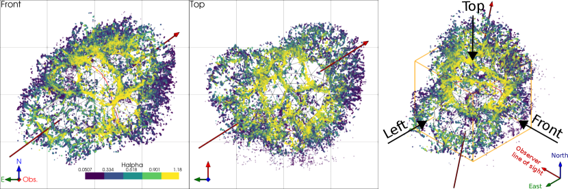
Figure 8: Front (as seen from Earth) and top view of the H$\alpha$ emission. The right panel displays an isometric representation of the nebula showing the different viewpoints considered in the paper. The central part is filled with the inner envelope (see section 4.1.2) so that the rear-facing components are obscured. The red arrow represents the pulsar torus axis and the red line shows the intersection of the inner surface with the pulsar torus plane as fitted by Ng & Romani (2004). All axes are in parsecs and the spatial grid of the left and central panels has a 1 pc stepping. The orientation symbol is color coded: East is green, North is blue and the line-of-sight direction is red.

To construct a 3D mapping of the Crab Nebula we require an estimate of its distance. We adopt 2 kpc, computed by Trimble (1973), who estimates it to lie between 1.7 kpc and 2.4 kpc from prior morphological considerations. This distance has not been improved since then and is still in use in recent articles (see e.g., Hester 2008; Kaplan et al. 2008). At this distance 1 ″=9.696$\times 10^{-3}$ pc and the radial distance $d$ to the expansion center can be computed from the radial velocity $v_{r}$ via the expansion factor (Ng & Romani, 2004):

$$d=\frac{v_{r}}{e}$$ (13)

Knowing the expansion factor and the distance to the Crab makes it possible to obtain a mapping of our data in the Euclidean space (in parsecs) as shown in Figure 8 and appendix B. Given the complexity of our data we have created an interactive visualization in Python accessible through a Jupyter Notebook. It may be found at https://github.com/thomasorb/M1_paper. The 3D visualization program can also be run directly in any html browser at https://mybinder.org/v2/gh/thomasorb/M1_paper/master and does not require any particular computing knowledge.

Two movies have been created with the help of panda3d, an open-source framework for 3D rendering (Goslin & Mine, 2004). They are available online as supplementary material. Both show the total flux emitted in all 5 emission lines. Each data point is represented as a small cube and corresponds to one velocity component at a given pixel. No data points have been added by interpolation. The thickness of some of the brightest filaments along the line of sight comes from the fact that they could be resolved and fitted with two components instead of one. The Milky Way background has been adequately positioned to simulate what would be the typical perspective of someone moving around the nebula. The Milky Way map has been created by the NASA/Goddard Space Flight Center Scientific Visualization Studio (https://svs.gsfc.nasa.gov/4851) based in part on the data obtained with Gaia (Brown et al., 2018). One of the movies shows a glowing sphere at the center to simulate the blue continuum emitted by the pulsar wind nebula with an intensity to roughly match that observed in the composite HST image presented by Loll et al. (2013). The soundtrack is a sonification of the data set. Using the interferograms directly as a sound wave, we have mixed multiple samples played at different rates. The volume of the samples is related to the square of the distance to the nebula and the playing speed is related to the velocity of the observer with respect to the nebula. A second movie highlights the geometry of the Crab Nebula. The obtained data is shown with the inner and outer envelopes described in the next section. The pulsar axis and the plane of the pulsar torus are indicated.

4 Morphology of the Crab Nebula

4.1 Inner and outer envelopes

4.1.1 Outer envelope

Each of the H$\alpha$, [N ii]$\lambda\lambda$ 6548, 6584, and [S ii]$\lambda\lambda$6716, 6731 3D maps we have created is a collection of volume elements (voxels) that occupy the same volume in space and for which we can measure an emission line flux. This volume is bounded by the surface of 1 pixel at the distance of the nebula (0.32 ″ at 2 kpc i.e., $3.1\times 10^{-3}$ pc) and an element of spectral resolution along the line of sight (35 km s^-1 i.e. $3.1\times 10^{-2}$ pc), which yields a voxel volume of $3.0\times 10^{-7}$  pc³.

Representing our observations as voxels in this way provides a detailed representation of the Crab’s complex distribution of material and permits an investigation of its morphology at small and large scales. For example, it is worth testing whether or not the Crab is an ellipsoid, as long suspected (e.g., Hester 2008). To this end we can analyse the radial distribution of the emitting material contained in a solid angle originating from the explosion center and obtain the radial extent of the nebula by computing the outer limit of this distribution in all directions. To illustrate, we show in Figure 9 the distribution of material integrated over all directions along the pulsar torus axis. We see that no material extends beyond 2 pc.

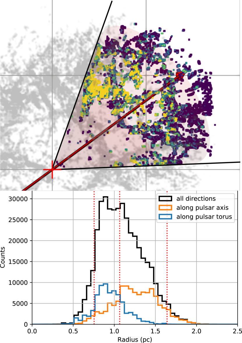
Figure 9: Representation of the emitting material contained in a solid angle originating from the explosion center and aligned along the pulsar axis. All axes are in parsecs and the spatial grid has a 1 pc stepping.

Because the emission $I(\textup{H$\alpha$})$ is very roughly proportional to the square of the ionized hydrogen density $n_{p}$ (at a constant temperature along the line of sight), $I(\textup{H$\alpha$})\propto n_{p}^{2}$, we choose to weight this distribution by $\sqrt{I(\textup{H$\alpha$})}$ in order to approximately sample the distribution of the material density.

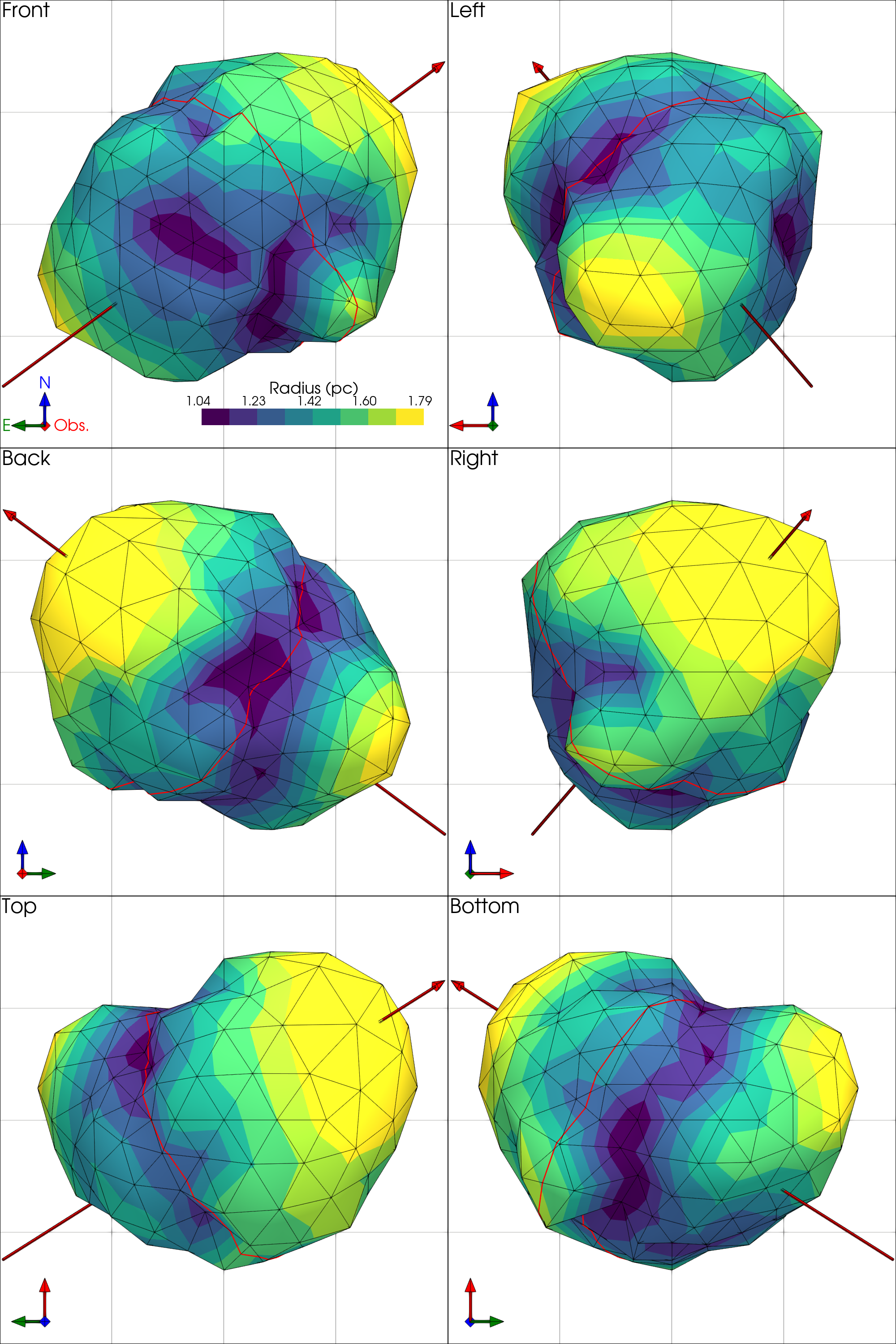
Figure 15: Outer envelope related to Figure 10. All 6 viewing angles are shown. Details are the same as Figure 8 and 10. The orientation symbol is color coded: East is green, North is blue and the line-of-sight direction is red.

We define the outer limit of the nebula in one particular direction as the radius that encompasses 97% of the material emitting in H$\alpha$ which is contained in a solid angle of 22.5^∘. We repeat this procedure over all directions, using the coordinates of the vertices of a 320-faced icosphere which ensures an homogeneous distribution of the probing directions (see appendix 17 for more details). Consequently, we obtain the outer envelope of the emitting material, i.e., the dominant shape of the Crab as made up by its visible gas. Two perspectives of this outer limit surface are shown in Figure 10, and all six perspectives are shown in Figure 15.

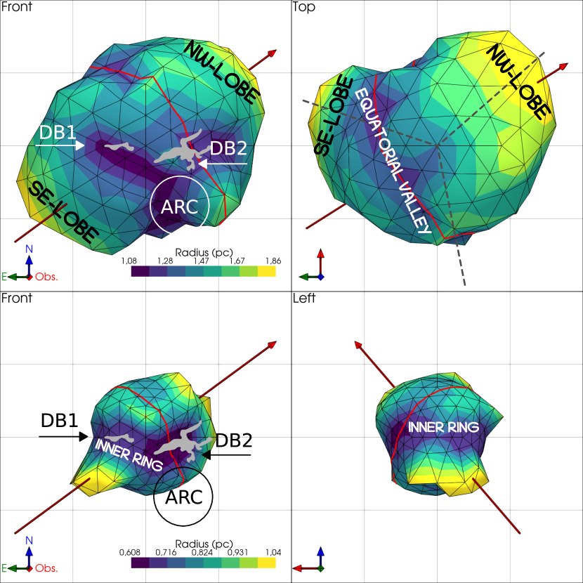
Figure 10: Top: Outer envelope enclosing 97% of the material emitting in H$\alpha$. The binning angle covers 22.5^∘. Bottom: Inner envelope enclosing 8% of the material emitting in H$\alpha$. The binning angle covers 45^∘. The positions of the dark bays (Fesen et al., 1992) and the arcade region (Dubner et al., 2017) are shown as well as the High-Helium bands first observed by Uomoto & MacAlpine (1987b) (in gray). We have also reported the topologic features referenced in the text. Other details are the same as Figure 8.

Note that, doing this in the plane of the sky and considering only the red part of the visible spectrum would reveal the well known elliptical outer envelope of the Crab. But the 3D outer envelope is most surprising since it differs notably from the generally assumed ellipsoidal shape (e.g., Hester 2008). As viewed from the top, which we define as being along the axis perpendicular to the observer’s line of sight looking from the north toward the south, a conspicuous heart-shaped morphology oriented along the pulsar axis is visible. The most rapidly expanding NW and SE lobes are separated by 120^∘ of each other. The NW lobe is nearly aligned with the pulsar torus axis, but the SE lobe is not.

The potential effects of inhomogeneities of the expansion factor must be considered since this spatial reconstruction is mostly based on a homologous expansion hypothesis (i.e., a constant expansion factor in all directions) which is not absolutely true. Using the data obtained by Trimble (1968), we find that the expansion is indeed accelerated towards the north-west direction by a factor of 15 % with respect to the median value of the expansion factor ($e=1.160(15)\times 10^{-3}$ year^-1) computed by Nugent (1998) and used in this article to derive the 3D model of the nebula (see Figure 11). Of course, this accelerated expansion is associated with a dilatation of the ellipsoidal shape of the nebula in the same direction. Knowing only the proper motion of the nebula and using a homologous expansion model to compute its shape, one would have exaggerated this dilatation effect, resulting in a nebula with an envelope even more extended towards the north-east direction. We have fitted an ellipsoid to the computed outer envelope and obtained the dilatation ratio. The center of the ellipsoid coincides with the center of expansion and its major axis follows the axis of the pulsar torus. As shown in Figure 11, the dilatation ratio of the SE-Lobe (which gives its heart shape to the nebula) is around 1.3. It would require an expansion inhomogeneity of the same order to keep the model compatible with an ellipsoid, which is two times larger than what is observed in the celestial plane. Moreover, this expansion inhomogeneity should not be related with any extension of the nebula in this direction, which is in contradiction with the correlation we observed based on Trimble (1968) data. We are thus confident that, if the computed 3D model of the nebula might indeed be exaggerated along the line-of-sight, the general shape should not differ enough to make it completely compatible with an ellipsoid.

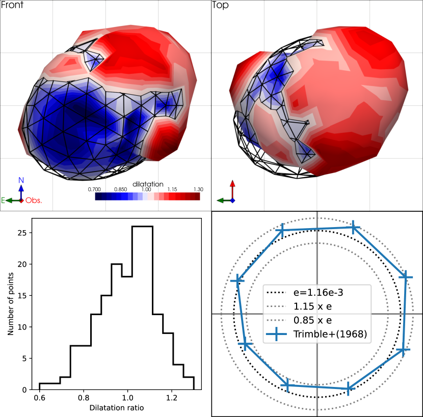
Figure 11: Top: Ellipsoid (wireframe) fitted to the outer envelope. The ellipsoid represents the surface of dilatation factor unity. Its center coincides with the center of expansion and its major axis follows the axis of the pulsar torus. The color of the outer envelope represents its dilatation factor. Regions above the ellipsoid are red while regions below are blue. All axes are in parsecs and the spatial grid has a 1 pc stepping. The orientation symbol is color coded: East is green, North is blue and the line-of-sight direction is red.Bottom-left: Histogram of the dilatation of the outer envelope with respect to the fitted ellipsoid. Bottom-right: median of the expansion factor measured by Trimble (1968) along different directions (north is up and east to the left). The circles of homologous expansion are represented with dotted lines. The north-west acceleration appears clearly and can be related to the dilatation along the north-west lobe but there is no acceleration as high as the 1.3 dilatation factor observed in the SE-Lobe. Even if we consider the largest expansion factor measured in the plane of the sky (1.15), this is not sufficient to explain the factor 1.3 dilatation observed in the south-west lobe.

4.1.2 Inner envelope

The Crab shows an intricate complex of filamentary structures going deep under its outer envelope, and it can be difficult to easily identify 3D locations of material. Thus, it is of interest to define the inner extent of this material, i.e. the size and the morphology of the central void of ionized gas around the center of expansion, to distinguish front-facing from rear-facing ejecta. If we look at the distribution of material and integrate over all directions (Figure 9) we see that no material is located below 0.5 pc. However, we take this a step further by examining the 3D extent of this void in all directions. Using the same procedure as the one used to obtain the outer envelope, we obtained the inner envelope considering a radius enclosing only 8% of the material emitting in H$\alpha$ in a solid angle of 45^∘. The limit of 8 % may seem high but is explained by the relatively high number of spurious detections near the center. We have thus slowly increased the limit up to the point where the 3D shape of the inner surface was not changing anymore (except for its scale). Two perspectives of this inner limit surface are shown in Figure 10, and all six perspectives are shown in Figure 16.

4.1.3 Comparison of the inner and outer envelopes

Comparing the inner and outer envelopes reveals clear trends in the overall morphology of gas. Material around the plane defined by the pulsar torus mapped by Ng & Romani (2004) is much closer to the explosion center than the material distributed along the pulsar axis. This can be seen as a circular pinched valley running along the pulsar torus plane (labeled equatorial valley). On the front of the nebula two small depressions are seen (labeled DB1 and DB2 on the figure) that coincide with the pinched velocity regions observed by MacAlpine et al. (1989a) and the helium-rich bands observed by Uomoto & MacAlpine (1987b). Another indentation is seen in the general region of the “arcade of loops” described by Dubner et al. (2017). The two depressions DB1 and DB2 also coincide with the positions of the dark bays, (Fesen et al., 1992), also observed in the X-ray (Seward et al., 2006), and UV (see e.g., Dubner et al. 2017). Interestingly, the locations of the dark bays also coincide with a conspicuous restriction oriented along the east-west plane running along the perimeter of the inner envelope (labeled inner ring). Together, these shared features between the inner and outer envelopes strongly suggest a constrained expansion of the nebular material, potentially due to interaction with a pre-existing circumstellar disk left by the progenitor star (Fesen et al., 1992; Smith, 2013).

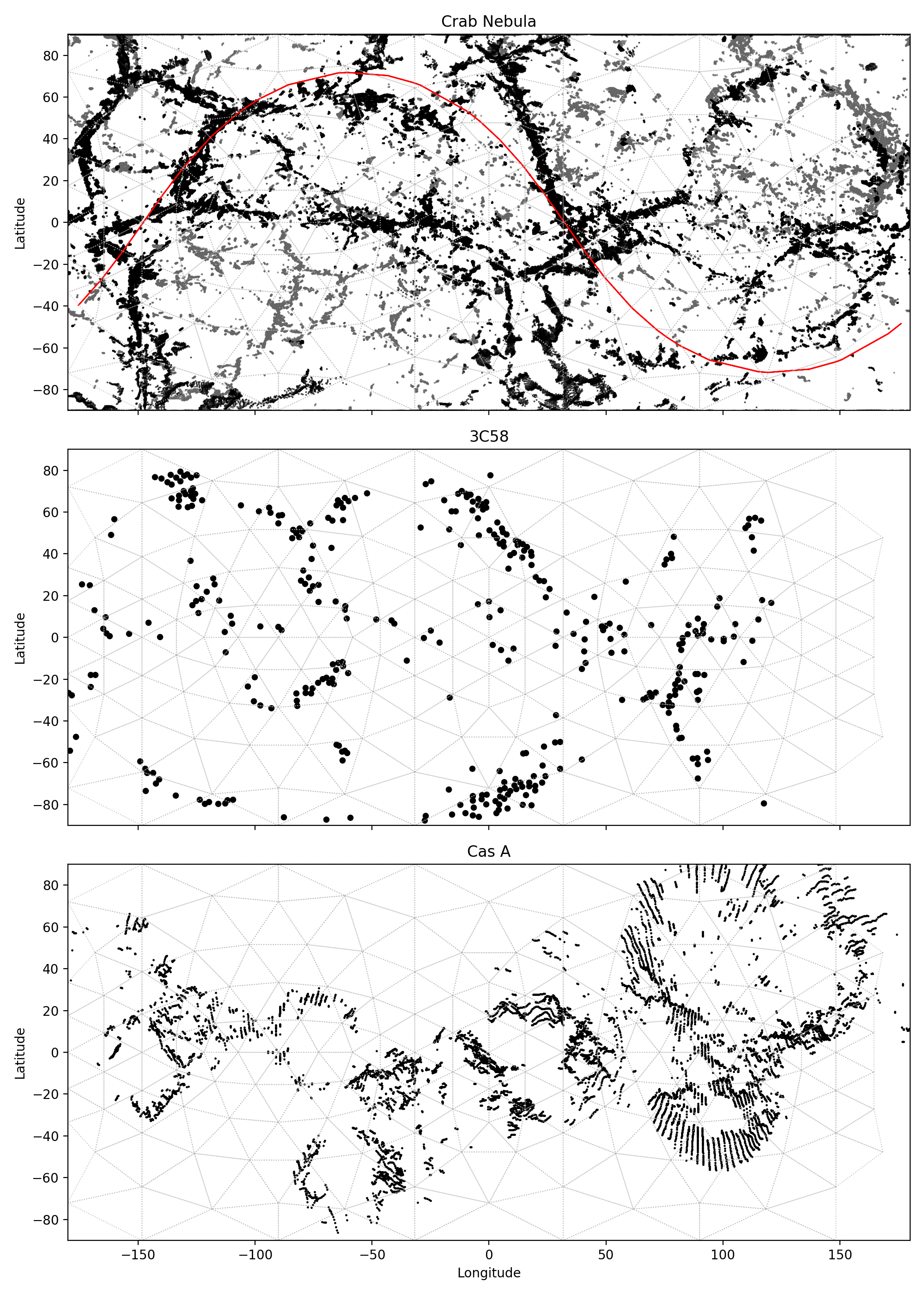
Figure 12: Top: Mercator projection of total flux of the emitting material in the Crab. The densest and deepest buried material (at less than 1.1 pc of the center) is represented in black while the faster expanding material is in gray. As the angles are not conserved, we overplot a grid of triangles which vertices sides cover an angle of 16.6^∘($\simeq\pi/11$). The red line shows the pulsar torus plane as fitted by Ng & Romani (2004). The center of the latitude and longitude axes corresponds to the center of expansion in the face-on view. Longitude increases towards the West. Middle and bottom: Mercator projections of 3C 58 (Lopez & Fesen, 2018), and Cas A (Milisavljevic & Fesen, 2013), respectively.

4.2 Filamentary structure

High resolution images of the Crab show that its filaments exhibit a complex and fine structure (see, e.g., Hester et al. 1996, Blair et al. 1997, and Sankrit et al. 1998). Many filaments are less than an arcsecond in width and point inward into the center of the nebula, with lengths ranging from $\approx 1^{\prime\prime}-20^{\prime\prime}$. Filaments are also often connected by arc-like bridges of emission with a “bubble-and-spike” morphology (Hester, 2008). Numerous studies have associated this morphology with Rayleigh-Taylor (RT) instabilities (see for example Chevalier & Gull 1975; Hester et al. 1996; Bucciantini et al. 2004; Stone & Gardiner 2007; Porth et al. 2014). These instabilities are generally characterized by 2 parameters. (1) Angular size, i.e., the wavelength of the perturbations, which is strongly related to the stability of the shell. Numerical MHD simulations (Bucciantini et al., 2004) show that only perturbations at a scale smaller than $\sim\pi/10$ should give rise to RT instabilities and to the observed structures with protruding fingers. (2) The size of the filaments, which should also be related to the wavelength of these perturbations.

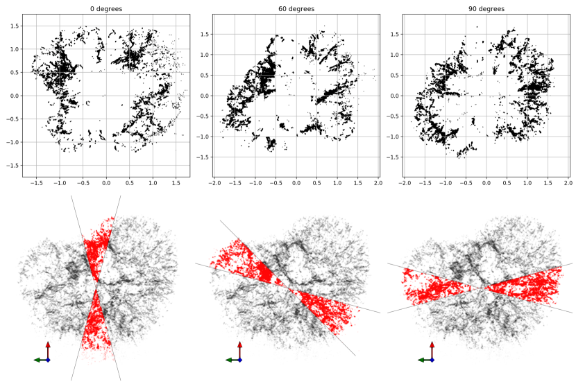
Figure 13: Slices in 3 different directions with respect to the line of sight direction. The slice at 90^∘ beeing the canonical point of view perpendicular to the line of sight. All points at $\pm$15^∘are merged together so that the angular size of a slice is 30^∘. A top view of the selected pixels is shown at the bottom. It shows the slice extent used to generate the plots in the corresponding upper panel. Axes are in pc. The orientation symbol is color coded: East is green, North is blue and the line-of-sight direction is red.

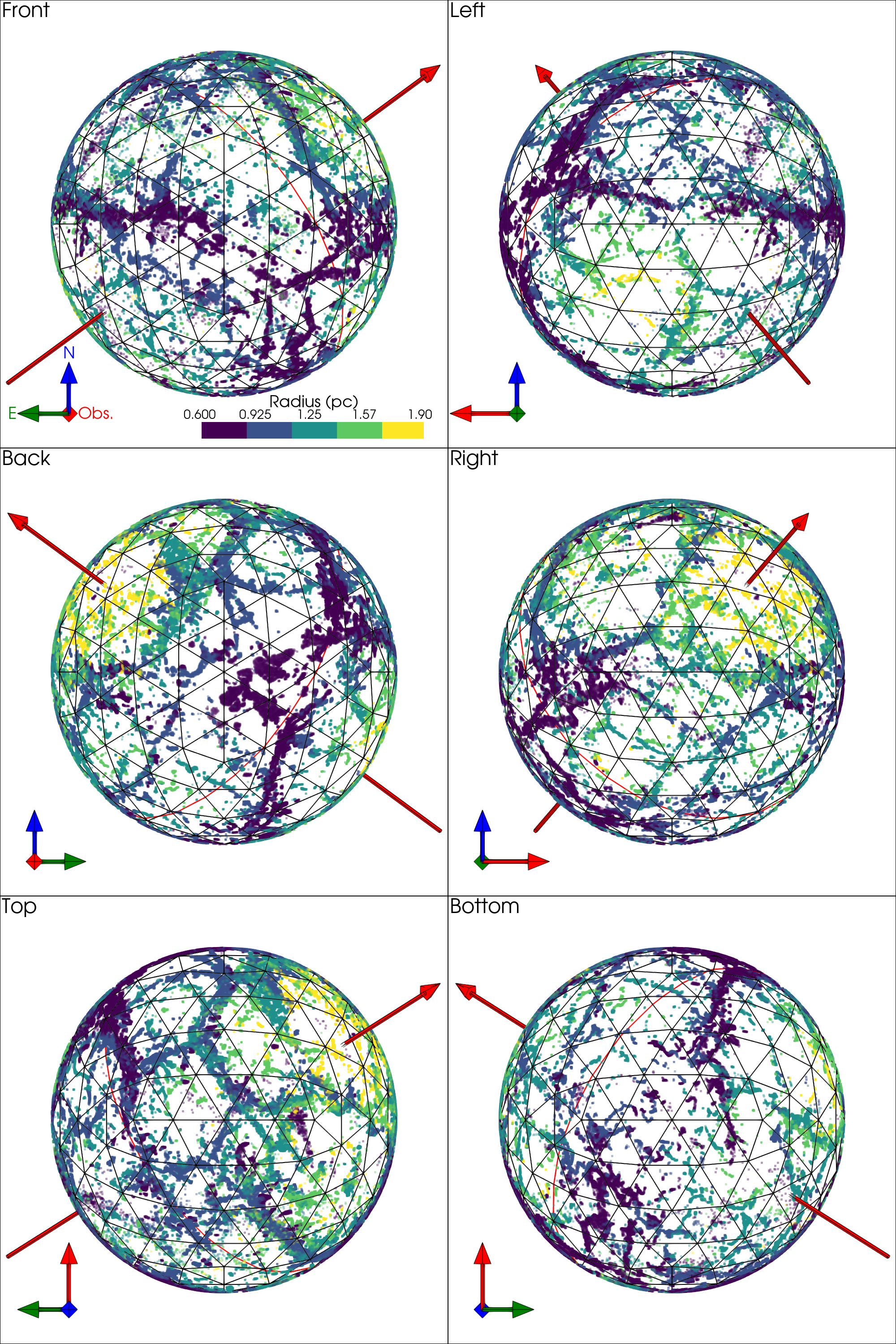
Figure 18: Orthographic projections of all the voxels at the same unit radius to reveal the structuration of the filamentary envelope of the nebula. This is presented as an alternative to Mercator projections shown in Figure 12 which produce important distortions far from the equator. A grid of triangles with 16.6^∘($\simeq\pi/11$) sides helps to measure the size of the structures. The red arrow indicates the direction of the pulsar torus and the red line shows its equator. The orientation symbol is color coded: East is green, North is blue and the line-of-sight direction is red.

In Figure 12 we show the whole structure as if all voxels were at the same radius in a classical Mercator projection, and in Figure 18 as orthographic projections. All maps are gridded with triangles having sides covering an angle of 16.6^∘($\simeq\pi/11$), which is helpful to measure the relative sizes of the different structures.

Crab material is largely distributed along boundaries resembling a honeycomb. This structure is hierarchical; i.e., larger regions ($\sim\pi/3.5$) have thicker filaments, while other regions, in particular in the high-velocity lobes, exhibit a much smaller and thinner distribution ($\sim\pi/10$). The interior of the largest structures is generally divided into smaller regions that are also at a larger radii. The size of the structures appear to be anti-correlated with the radius; i.e., the largest and most conspicuous structures are at smallest radii with smallest expansion velocities. Some of the largest structures, seen clearly on the top and back views of Figure 12, exhibit a polygonal shape and are found all along the pulsar torus equatorial plane. One also sees these structures when viewing the Crab through narrow slices along different orientations (Figure 13). The largest regions are localized in the interior with diameters of 0.5 to 1 pc. Above these at larger radii lie numerous smaller bubbles.

5 Discussion

There exist very few kinematic maps of supernova remnants detailed enough that a comparison of the shape of their filamentary structure can be studied. Figure 12 shows a comparison of the mercator projections of the Crab, 3C 58 (Lopez & Fesen, 2018) and Cas A (Milisavljevic & Fesen, 2013). Large-scale ejecta rings may be a common phenomenon of young, core-collapse SNRs (Milisavljevic & Fesen, 2017). The largest and deepest structures of the Crab are similar both in size and shape as those seen in 3C 58. However, both the Crab and Cas A share small scale circular formations.

3C 58 has many overlapping properties with the Crab. The Crab Nebula is far brighter and more luminous than 3C 58, but both remnants are bright in both the radio and X-rays in their center and harbor young, rapidly spinning central pulsars that provide the magnetic field and relativistic particles that generate the observed center-filled synchrotron radiation. 3C 58 may be connected to the historical event of 1181 CE (Stephenson & Green, 2002; Kothes, 2013), which would make it only 127 years younger than the Crab. However, this relatively young age is inconsistent with its overall angular size ($6.3^{\prime}\times 10.3^{\prime}$) and proper motion measurements of its expanding ejecta (Fesen et al., 1988; van den Bergh, 1990) that suggest a much older remnant, potentially as old as $2400\pm 500$ yr.

Cas A is the youngest known core-collapse remnant with an estimated explosion date of 1681 CE (Fesen et al., 2006). Milisavljevic & Fesen (2013) demonstrated that the bulk of the remnant’s main shell ejecta are arranged in several well-defined complete or broken ring-like structures. These ring structures have diameters that can be comparable to the radius of the remnant ($\sim 1$ pc). Some rings show considerable radial extensions giving them a crown-like appearance, while other rings exhibit a frothy, ring-like substructure on scales of $\sim 0.2$ pc. A subsequent three-dimensional map of its interior unshocked ejecta made from near-infrared observations sensitive to [S III] $\lambda\lambda$ 9069, 9531 emission lines revealed a bubble-like morphology that smoothly connects with these rings (Milisavljevic & Fesen, 2015).

In the case of Cas A, the rings of ejecta have been interested to be the cross sections of reverse-shock-heated cavities in the remnant’s internal ejecta (Milisavljevic & Fesen, 2013). A cavity-filled interior is in line with prior predictions for the arrangement of expanding debris created by a post-explosion input of energy from plumes of radioactive ⁵⁶Ni-rich ejecta (Li et al., 1993; Blondin et al., 2001). Such plumes can push the nuclear burning zones located around the Fe core outward, creating dense shells separating zones rich in O, S, and Si from the Ni-rich material. After the SN shock breakout additional energy input from the radioactive decay of ⁵⁶Ni continues to drive inflation of ⁵⁶Ni-rich structures and facilitates mixing between ejecta components. This late time expansion can modify the overall SN ejecta morphology on timescales of weeks or months. Compression of surrounding nonradioactive material by hot expanding plumes of radioactive ⁵⁶Ni-rich ejecta generates a “Swiss cheese”-like structure that is frozen into the homologous expansion when the radio- active power of ⁵⁶Ni is strongest. Gabler et al. (2020) found that this “Ni-bubble effect” accelerates the bulk of the nickel in their 3D models and causes an inflation of the initially overdense Ni-rich clumps, which leads to underdense, extended fingers, enveloped by overdense skins of compressed surrounding matter.

Stockinger et al. (2020) recently performed 3D full-sphere simulations of supernovae originating from non-rotating progenitors similar to those anticipated to be associated with the SN 1054. Their low energy explosions ($\sim 0.5-1.0\times 10^{50}$ erg) are compared in two contrasting scenarios: (1) iron-core progenitors at the low-mass end of the core-collapse supernova domain ($\approx 9$ M_⊙), and (2) a super-AGB progenitor with an oxygen-neon-magnesium core that collapses and explodes as electron-capture supernova. They disfavor associating SN 1054 with an electron capture supernova because the kick experienced by the neutron star is negligible and inconsistent with the observed $\approx 160$ km s^-1 transverse velocity of Crab pulsar. Instead, they favour simulations with iron-core progenitors with less 2nd dredge-up that result in highly asymmetric explosions with hydrodynamic and neutrino-induced NS kick of $>40$ km s^-1 and a NS spin period of $\sim 30$ ms, not unlike the Crab pulsar. The resulting distribution of ⁵⁶Ni-rich material from these explosions, which enable efficient mixing and dramatic shock deceleration in the extended hydrogen envelope, is potentially consistent with our mapping of Crab ejecta. However, simulations extending the evolution from $\sim$ days to $\sim$ 1000 years are needed to verify this extrapolation (see, e.g., Orlando et al. 2016).

6 Conclusions

We have presented a 3D kinematic reconstruction of the Crab Nebula that has been created from a hyperspectral cube obtained with SITELLE. The data is comprised of 310 000 high resolution ($R=9\,600$) spectra containing H$\alpha$, [N ii], and [S ii] line emission, and represent the most detailed homogeneous spectral data set ever obtained of the Crab Nebula.

Our findings can be summarized as follows:

1. The general shape of the Crab, as measured by 97% of the material emitting in H$\alpha$, occupies a “heart-shaped” volume and is symmetrical about the plane of the pulsar wind torus. This morphology runs counter to the generally assumed ellipsoidal volume and is not an artifact of assuming a uniform global expansion. The most rapidly expanding NW and SE lobes are separated by 120^∘ of each other. The NW lobe is nearly aligned with the pulsar torus axis, but the SE lobe is not.

2. Conspicuous restrictions in the distribution of material as mapped by the inner and outer limits of emission is seen along the band of He-rich filaments (Uomoto & MacAlpine, 1987b; MacAlpine et al., 1989b). Notable depressions are also coincident with the east and west dark bays (Fesen et al., 1992). Together these features are consistent with constrained expansion of Crab ejecta, possibly associated with interaction between the supernova and a pre-existing cirumstellar disk.

3. The filaments follow a honeycomb-like distribution defined by a combination of straight and rounded boundaries at large and small scales. The scale size is anti-correlated with distance from the center of expansion; i.e., largest features are found at smallest radii. The structures are not unlike those seen in other SNRs, including 3C 58 and Cas A, where they have been attributed to turbulent mixing processes that encouraged outwardly expanding plumes of radioactive ⁵⁶Ni-rich ejecta.

The observed kinematic characteristics reflect critical details concerning the original supernova of 1054 CE and its progenitor star, and may favour a low-energy explosion of an iron-core progenitor as opposed to an oxygen-neon-magnesium core that collapses and explodes as an electron-capture supernova. Planned future observations will provide additional hyperspectral cubes spanning more wavelength windows that include the emission lines of [O II] $\lambda\lambda$3726, 3729, H$\beta$, [O III] $\lambda\lambda$4959, 5007, [N II] $\lambda$5755, and He I $\lambda$5876. These lines will be measured and modeled to determine temperature, density and abundances at very fine scales, and combined with an updated proper motion investigation of filaments (Martin et al., in preparation) to improve the accuracy of our reconstruction at fine scales. Our work contributes to a larger suite of detailed supernova remnant reconstructions being developed that will provide unique constraints for increasingly sophisticated three-dimensional core-collapse simulations (Couch et al., 2015; Wongwathanarat et al., 2017; Burrows et al., 2019; Stockinger et al., 2020), that are being evolved to middle-aged supernova remnants (Orlando et al., 2015, 2016; Orlando et al., 2020), attempting to model the complete multi-messenger signals of supernovae (Andresen et al., 2017; Kuroda et al., 2017; Westernacher-Schneider et al., 2019; Mezzacappa et al., 2020).

Data availability

The data underlying this article will be shared on reasonable request to the corresponding author.

Appendix A Velocity Uncertainty

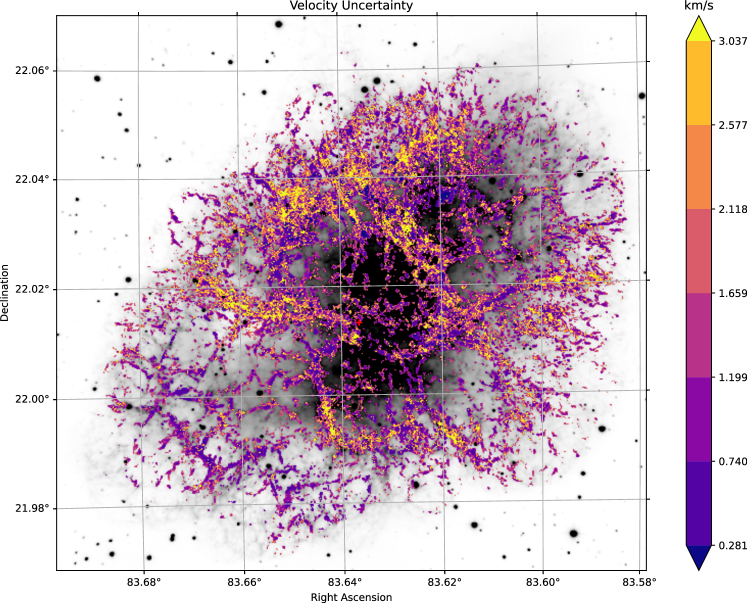
Figure 14: Map of the velocity uncertainty related to Figure 7. The uncertainty is an output of the fit realised with ORCS (Martin et al., 2015). It is calculated from the covariance matrix returned by the Levenberg-Marquardt minimization process (Levenberg, 1944; Marquardt, 1963). As all 5 emission-lines for each velocity component share the same velocity parameter, the uncertainty is generally smaller that the uncertainty that would have been obtained by fitting the emission-lines independently. As other constraints are implemented in the spectrum model (see section 3.3) the emission-lines velocities and fluxes are the parameters of one spectrum model. As such their uncertainty are only loosely related to the SNR of each emission-line (see Martin et al. 2015 for more details).

Appendix B 3d maps

Figure 16: Inner envelope related to Figure 10. All 6 viewing angles are shown. Details are the same as Figure 8 and 10. The orientation symbol is color coded: East is green, North is blue and the line-of-sight direction is red.

Appendix C Icosphere

Figure 17: Icosahedron (a, 20 faces), subdivided 2 times along its edges to make the 80 (b) and 320 faces (c) icospheres. This type of sphere approximation is interesting since its vertices are homogeneously distributed. We used the 320 icosphere to construct the inner and outer envelope as well as to make a homogeneous grid on the projections of Figures 12 and 18.

Appendix D Filamentary structure

References

- Alarie et al. (2014) Alarie A., Bilodeau A., Drissen L., 2014, MNRAS, 441, 2996
- Andresen et al. (2017) Andresen H., Müller B., Müller E., Janka H. T., 2017, MNRAS, 468, 2032
- Baril et al. (2016) Baril M. R., et al., 2016, in Evans C. J., Simard L., Takami H., eds, Proceedings of SPIE. International Society for Optics and Photonics, p. 990829
- Bennett (2000) Bennett C. L., 2000, Imaging the Universe in Three Dimensions. Proceedings from ASP Conference Vol. 195. Edited by W. van Breugel and J. Bland-Hawthorn. ISBN: 1-58381-022-6 (2000), 195
- Bietenholz & Nugent (2015) Bietenholz M. F., Nugent R. L., 2015, Monthly Notices of the Royal Astronomical Society, 454, 2416
- Black & Fesen (2015) Black C. S., Fesen R. A., 2015, MNRAS, 447, 2540
- Blair et al. (1997) Blair W. P., Davidson K., Fesen R. A., Uomoto A., MacAlpine G. M., Henry R. B. C., 1997, ApJS, 109, 473
- Blondin et al. (2001) Blondin J. M., Borkowski K. J., Reynolds S. P., 2001, ApJ, 557, 782
- Brown et al. (2018) Brown A. G. A., et al., 2018, Astronomy & Astrophysics, 616, A1
- Bucciantini et al. (2004) Bucciantini N., Amato E., Bandiera R., Blondin J. M., Del Zanna L., 2004, Astronomy & Astrophysics, 423, 253
- Burrows et al. (2019) Burrows A., Radice D., Vartanyan D., 2019, MNRAS, 485, 3153
- Charlebois et al. (2010) Charlebois M., Drissen L., Bernier A. P., Grandmont F., Binette L., 2010, AJ, 139, 2083
- Chevalier (1977) Chevalier R. A., 1977, in Schramm D. N., ed., Astrophysics and Space Science Library, Vol. 66, Supernovae. p. 53, doi:10.1007/978-94-010-1229-4_5
- Chevalier & Gull (1975) Chevalier R. A., Gull T. R., 1975, ApJ, 200, 399
- Chugai & Utrobin (2000) Chugai N. N., Utrobin V. P., 2000, A&A, 354, 557
- Clark & Stephenson (1977) Clark D. H., Stephenson F. R., 1977, The historical supernovae
- Couch et al. (2015) Couch S. M., Chatzopoulos E., Arnett W. D., Timmes F. X., 2015, ApJ, 808, L21
- Davidson & Fesen (1985) Davidson K., Fesen R. A., 1985, ARA&A, 23, 119
- DeLaney et al. (2010) DeLaney T., et al., 2010, ApJ, 725, 2038
- Drissen et al. (2019) Drissen L., et al., 2019, MNRAS, 485, 3930
- Dubner et al. (2017) Dubner G., Castelletti G., Kargaltsev O., Pavlov G. G., Bietenholz M., Talavera A., 2017, The Astrophysical Journal, 840, 82
- Fesen et al. (1988) Fesen R. A., Kirshner R. P., Becker R. H., 1988, in Roger R. S., Landecker T. L., eds, IAU Colloq. 101: Supernova Remnants and the Interstellar Medium. p. 55
- Fesen et al. (1992) Fesen R. A., Martin C. L., Shull J. M., 1992, The Astrophysical Journal, 399, 599
- Fesen et al. (1997) Fesen R. A., Shull J. M., Hurford A. P., 1997, The Astronomical Journal, 113, 354
- Fesen et al. (2006) Fesen R. A., et al., 2006, The Astrophysical Journal, 645, 283
- Gabler et al. (2020) Gabler M., Wongwathanarat A., Janka H.-T., 2020, arXiv e-prints, p. arXiv:2008.01763
- Gessner & Janka (2018) Gessner A., Janka H.-T., 2018, ApJ, 865, 61
- Goslin & Mine (2004) Goslin M., Mine M. R., 2004, Computer, 37, 112
- Grefenstette et al. (2017) Grefenstette B. W., et al., 2017, ApJ, 834, 19
- Hester (2008) Hester J. J., 2008, Annual Review of Astronomy and Astrophysics, 46, 127
- Hester et al. (1996) Hester J. J., et al., 1996, The Astrophysical Journal, 456, 225
- Hillebrandt (1982) Hillebrandt W., 1982, A&A, 110, L3
- Hunter (2007) Hunter J. D., 2007, Computing in science & engineering, 9, 90
- Högbom (1974) Högbom J. A., 1974, Astronomy and Astrophysics Supplement Series, 15, 417
- Kaplan et al. (2008) Kaplan D. L., Chatterjee S., Gaensler B. M., Anderson J., 2008, The Astrophysical Journal, 677, 1201
- Kitaura et al. (2006) Kitaura F. S., Janka H. T., Hillebrandt W., 2006, A&A, 450, 345
- Kothes (2013) Kothes R., 2013, Astronomy & Astrophysics, 560, A18
- Kuroda et al. (2017) Kuroda T., Kotake K., Hayama K., Takiwaki T., 2017, ApJ, 851, 62
- Law et al. (2020) Law C. J., et al., 2020, ApJ, 894, 73
- Lawrence et al. (1995) Lawrence S. S., MacAlpine G. M., Uomoto A., Woodgate B. E., Brown L. W., Oliversen R. J., Lowenthal J. D., Liu C., 1995, AJ, 109, 2635
- Levenberg (1944) Levenberg K., 1944, Quarterly of Applied Mathematics, 2, 164
- Li et al. (1993) Li H., McCray R., Sunyaev R. A., 1993, ApJ, 419, 824
- Loll et al. (2013) Loll A. M., Desch S. J., Scowen P. A., Foy J. P., 2013, The Astrophysical Journal, 765, 152
- Lopez & Fesen (2018) Lopez L. A., Fesen R. A., 2018, The Morphologies and Kinematics of Supernova Remnants (arXiv:1804.00024), doi:10.1007/s11214-018-0481-x, https://link.springer.com/article/10.1007/s11214-018-0481-x
- Lundqvist & Tziamtzis (2012) Lundqvist P., Tziamtzis A., 2012, MNRAS, 423, 1571
- MacAlpine et al. (1989a) MacAlpine G. M., McGaugh S. S., Mazzarella J. M., Uomoto A., 1989a, ApJ, 342, 364
- MacAlpine et al. (1989b) MacAlpine G. M., McGaugh S. S., Mazzarella J. M., Uomoto A., 1989b, The Astrophysical Journal, 342, 364
- Maillard et al. (2013) Maillard J. P., Drissen L., Grandmont F., Thibault S., 2013, Experimental Astronomy, 35, 527
- Marquardt (1963) Marquardt D. W., 1963, Journal of the Society for Industrial and Applied Mathematics, 11, 431
- Martin (2015) Martin T., 2015, Phd thesis, Université Laval
- Martin & Drissen (2016) Martin T., Drissen L., 2016, in Reylé C., Richard J., Cambrésy L., Deleuil M., Pécontal E., Tresse L., Vauglin I., eds, Proceedings of the annual meeting of the French Society of Astronomy & Astrophysics Lyon, June 14-17, 2016. pp 23–28
- Martin et al. (2012) Martin T., Drissen L., Joncas G., 2012, in Radziwill N. M., Chiozzi G., eds, Vol. 2, SPIE - Software and Cyberinfrastructure for Astronomy II. pp 84513K–84513K–9
- Martin et al. (2015) Martin T., Drissen L., Joncas G., 2015, Astronomical Data Analysis Software an Systems XXIV (ADASS XXIV), 495
- Martin et al. (2016) Martin T. B., Prunet S., Drissen L., 2016, Monthly Notices of the Royal Astronomical Society, 463, 4223
- McKinney et al. (2010) McKinney W., et al., 2010, in Proceedings of the 9th Python in Science Conference. pp 51–56
- Mezzacappa et al. (2020) Mezzacappa A., et al., 2020, Phys. Rev. D, 102, 023027
- Milisavljevic & Fesen (2013) Milisavljevic D., Fesen R. A., 2013, ApJ, 772, 134
- Milisavljevic & Fesen (2015) Milisavljevic D., Fesen R. A., 2015, Science, 347, 526
- Milisavljevic & Fesen (2017) Milisavljevic D., Fesen R. A., 2017, in Alsabti A. W., Murdin P., eds, , Handbook of Supernovae. p. 2211, doi:10.1007/978-3-319-21846-5_97
- Ng & Romani (2004) Ng C., Romani R. W., 2004, The Astrophysical Journal, 601, 479
- Nomoto (1987) Nomoto K., 1987, ApJ, 322, 206
- Nomoto et al. (1982) Nomoto K., Sparks W. M., Fesen R. A., Gull T. R., Miyaji S., Sugimoto D., 1982, Nature, 299, 803
- Nugent (1998) Nugent R. L., 1998, Publications of the Astronomical Society of the Pacific, 110, 831
- Oliphant (2006) Oliphant T. E., 2006, A guide to NumPy. Vol. 1, Trelgol Publishing USA
- Ono et al. (2020) Ono M., Nagataki S., Ferrand G., Takahashi K., Umeda H., Yoshida T., Orland o S., Miceli M., 2020, ApJ, 888, 111
- Orlando et al. (2015) Orlando S., Miceli M., Pumo M. L., Bocchino F., 2015, ApJ, 810, 168
- Orlando et al. (2016) Orlando S., Miceli M., Pumo M. L., Bocchino F., 2016, ApJ, 822, 22
- Orlando et al. (2020) Orlando S., Wongwathanarat A., Janka H. T., Miceli M., Ono M., Nagataki S., Bocchino F., Peres G., 2020, arXiv e-prints, p. arXiv:2009.01789
- Osterbrock & Ferland (2006) Osterbrock D., Ferland G., 2006, Astrophysics of gaseous nebulae and active galactic nuclei. University Science Books, Sausalito
- Porth et al. (2014) Porth O., Komissarov S. S., Keppens R., 2014, Monthly Notices of the Royal Astronomical Society, 443, 547
- Price-Whelan et al. (2018) Price-Whelan A. M., et al., 2018, The Astronomical Journal, 156, 123
- Sankrit et al. (1998) Sankrit R., et al., 1998, ApJ, 504, 344
- Seward et al. (2006) Seward F. D., Tucker W. H., Fesen R. A., 2006, The Astrophysical Journal, 652, 1277
- Smith (2013) Smith N., 2013, MNRAS, 434, 102
- Sollerman et al. (2000) Sollerman J., Lundqvist P., Lindler D., Chevalier R. A., Fransson C., Gull T. R., Pun C. S. J., Sonneborn G., 2000, ApJ, 537, 861
- Stephenson & Green (2002) Stephenson F. R., Green D. A., 2002, in Historical supernovae and their remnants.
- Stockinger et al. (2020) Stockinger G., et al., 2020, MNRAS, 496, 2039
- Stone & Gardiner (2007) Stone J. M., Gardiner T., 2007, The Astrophysical Journal, 671, 1726
- Sullivan & Kaszynski (2019) Sullivan C. B., Kaszynski A., 2019, Journal of Open Source Software, 4, 1450
- Tominaga et al. (2013) Tominaga N., Blinnikov S. I., Nomoto K., 2013, ApJ, 771, L12
- Trimble (1968) Trimble V., 1968, The Astronomical Journal, 73, 535
- Trimble (1973) Trimble V., 1973, Publications of the Astronomical Society of the Pacific, 85, 579
- Uomoto & MacAlpine (1987b) Uomoto A., MacAlpine G. M., 1987b, The Astronomical Journal, 93, 1511
- Uomoto & MacAlpine (1987a) Uomoto A., MacAlpine G. M., 1987a, AJ, 93, 1511
- Van Rossum & Drake (2009) Van Rossum G., Drake F. L., 2009, Python 3 Reference Manual. CreateSpace, Scotts Valley, CA
- Virtanen et al. (2020) Virtanen P., et al., 2020, Nature Methods,
- Vogt & Dopita (2010) Vogt F., Dopita M. A., 2010, ApJ, 721, 597
- Vogt et al. (2018) Vogt F. P. A., Bartlett E. S., Seitenzahl I. R., Dopita M. A., Ghavamian P., Ruiter A. J., Terry J. P., 2018, Nature Astronomy, 2, 465
- Westernacher-Schneider et al. (2019) Westernacher-Schneider J. R., O’Connor E., O’Sullivan E., Tamborra I., Wu M.-R., Couch S. M., Malmenbeck F., 2019, Phys. Rev. D, 100, 123009
- Wongwathanarat et al. (2017) Wongwathanarat A., Janka H.-T., Müller E., Pllumbi E., Wanajo S., 2017, ApJ, 842, 13
- Wyckoff & Murray (1977) Wyckoff S., Murray C. A., 1977, Monthly Notices of the Royal Astronomical Society, 180, 717
- Yang & Chevalier (2015) Yang H., Chevalier R. A., 2015, ApJ, 806, 153
- Čadež et al. (2004) Čadež A., Carramiñana A., Vidrih S., 2004, ApJ, 609, 797
- van den Bergh (1990) van den Bergh S., 1990, ApJ, 357, 138