MSED: A Multi-Modal Sleep Event Detection Model for Clinical Sleep Analysis

Abstract

Clinical sleep analysis require manual analysis of sleep patterns for correct diagnosis of sleep disorders. However, several studies have shown significant variability in manual scoring of clinically relevant discrete sleep events, such as arousals, leg movements, and sleep disordered breathing (apneas and hypopneas). We investigated whether an automatic method could be used for event detection and if a model trained on all events (joint model) performed better than corresponding event-specific models (single-event models). We trained a deep neural network event detection model on 1653 individual recordings and tested the optimized model on 1000 separate hold-out recordings. F1 scores for the optimized joint detection model were 0.70, 0.63, and 0.62 for arousals, leg movements, and sleep disordered breathing, respectively, compared to 0.65, 0.61, and 0.60 for the optimized single-event models. Index values computed from detected events correlated positively with manual annotations (r² = 0.73, r² = 0.77, r² = 0.78, respectively). We furthermore quantified model accuracy based on temporal difference metrics, which improved overall by using the joint model compared to single-event models. Our automatic model jointly detects arousals, leg movements and sleep disordered breathing events with high correlation with human annotations. Finally, we benchmark against previous state-of-the-art multi-event detection models and found an overall increase in F1 score with our proposed model despite a 97.5% reduction in model size. Source code for training and inference is available at https://github.com/neergaard/msed.git.

Computational sleep science, object detection, deep neural network

1 Introduction

Clinical sleep analysis is currently evaluated manually by experts based on guidelines from the American Academy of Sleep Medicine (AASM) detailed in the AASM Scoring Manual [1]. The guidelines detail both technical and clinical best practices for setting up and recording polysomnographies, which are overnight recordings of various electrophysiological signals including electroencephalography (EEG), electrooculography (EOG), chin and leg electromyography (EMG), electrocardiography (ECG), respiratory inductance plethysmography from the thorax and abdomen, oronasal pressure, and blood oxygen levels. Based on these signals, expert technicians score and analyse the PSG for sleep stages [ wakefulness (W), REM sleep, non- stage 1 (N1), non- stage 2 (N2), and non- stage 3 (N3)], and sleep micro-events summarized by key metrics, such as the number of apneas and hypopneas per hour of sleep (apnea-hypopnea index, AHI), the number of (periodic) leg movements per hour of sleep [(periodic) leg movement index, (P)LMI], and the number of arousals per hour of sleep (arousal index, ArI).

Ar are defined as abrupt shifts in EEG frequencies towards alpha, theta, and beta rhythms for at least $3\text{\,}\mathrm{s}$ with a preceding period of stable sleep of at least $10\text{\,}\mathrm{s}$ [2]. During REM sleep, where the background EEG shows similar rhythms, arousal scoring requires a concurrent increase in chin EMG lasting at least $1\text{\,}\mathrm{s}$ [1].

LM should be scored when there is an increase in amplitude of at least $8\text{\,}\mathrm{\SIUnitSymbolMicro V}$ in the leg EMG channels above baseline level with a duration between $0.5\text{\,}\mathrm{s}10\text{\,}\mathrm{s}$ [3]. A PLM series is then defined as a sequence of 4 leg movements, where the time between LM onsets is between $5\text{\,}\mathrm{min}90\text{\,}\mathrm{min}$ [1, 4].

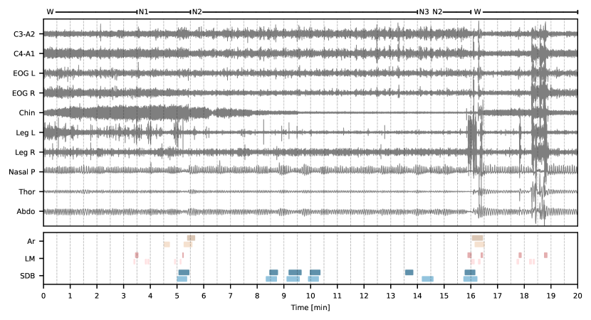
Figure 1: Example of MSED input and output predictions. Ten PSG channels comprising EEG, EOG, EMG, and breathing are visualized, which are fed to the MSED model. The bottom shows the manually scored (darker shade) and model predicted (lighter shade) events associated with the given recording segment. Sleep stages are shown at the top. W: wakefulness; N1: non- stage 1; N2: non- stage 2; N3: non- stage 3; Ar: arousal; LM: leg movement; SDB: sleep disordered breathing.

Apneas are generally scored when there is a complete ($\geq 90\text{\,}\mathrm{\char 37\relax}$ of pre-event baseline) cessation of breathing activity. The underlying cause can be either a physical obstruction (obstructive apnea) or due to an underlying disruption in the central nervous system control (central apnea) for at least $10\text{\,}\mathrm{s}$ [5]. When breathing is only partially reduced ($\geq 30\text{\,}\mathrm{\char 37\relax}$ of pre-event baseline) and the duration of the excursion is $\geq 10\text{\,}\mathrm{s}$, the event is scored as a hypopnea if there is either a $\geq 4\text{\,}\mathrm{\char 37\relax}$ oxygen desaturation or a $\geq 3\text{\,}\mathrm{\char 37\relax}$ oxygen desaturation coupled with an arousal [1]. SDB here refers to the collective of apneas and hypopneas.

Several studies have shown significant variability in the scoring of both sleep stages [6, 7, 8, 9, 10, 11, 12] and sleep micro-events [13, 14, 15, 16, 17, 18, 19, 5]. This has prompted extensive research into automatic methods for classifying sleep stages in large-scale studies [20, 21, 22, 23, 24, 25, 26, 27], while the research in automatic arousal [28, 29, 30] and LM [31] detection on a similar scale is limited, but has attracted increased focus as evidenced by the You Snooze You Win PhysioNet challenge from 2018 [32, 33]. [24] recently proposed a multi-task CNN/RNN combination model for the purpose of classifying sleep stages and predicting apnea-hypopnea index (AHI) and leg movement index (LMI) [24]. They trained their model on $9000$ PSG recordings from the Massachusetts General Hospital (MGH) and evaluated their model on a held-out MGH dataset consisting of $1000$ PSGs, and on $5804$ PSGs studies from the Sleep Heart Health Study (SHHS), yielding strong AHI/expert correlation values ($0.85$ on MGH, $0.77$ on SHHS) and LMI/expert correlation (0.79 on MGH). [30] published a CNN/RNN model for combined arousal and sleep/wake detection yielding an arousal detection F1 score of 0.79 on a test set of 1024 unique subjects [30], which was subsequently validated in two separate patient groups [34, 35]. Similarly, [31] proposed a CNN/RNN model for LM detection reporting an impressive F1 score of 0.77 on $348$ PSGs from the MrOS sleep study [31]. However, these models are all based on classifying windows of sleep data with subsequent manual fine-tuning and post-processing to combine events predicted in close-proximity windows, which incurs a human-factor bias.

Recently, [36] proposed the Dreem One Shot Event Detector (DOSED) algorithm for detecting sleep spindles and K-complexes in the sleep EEG [36], which was further developed for arousal and leg movement detection in subsequent publications by [28] [28, 37]. The advantage of this kind of approach is two-fold: first, the model is trained end-to-end to detect and classify events of any type, since there is no reliance on manual post-hoc processing of event predictions; and second, using a grid of default event windows (discussed in Section 3.2) allows durations of different time scales. However, as these models were only designed for either EEG-only events [36, 37], or did not investigate joint detection of events occurring across multiple modalities [28], there is still an unmet need for models capable of predicting events of multiple classes from multiple sensor types.

In this study, we extend the previous work in [36, 28, 37] and introduce the multi-modal sleep event detection (MSED) model for joint detection of sleep micro-events. The model combines multiple recording modalities from the PSG and recent advances in machine learning to not only classify arousals, LMs, and sleep disordered breathings, but also annotate them in the temporal domain without the need for post-hoc processing of predictions. An example of model predictions for a segment of PSG data is shown in Fig. 1, where the input signals are shown in the top box and manually scored/predicted events in the bottom box.

Our contributions are as follows:

• We propose the MSED, which is a CNN/RNN based model using disentangled feature extraction streams trained end-to-end for for multi-modal sleep event detection. To our knowledge, this is the first time this has been shown for multiple event types with multiple modalities trained simultaneously.

• We report inceased F1 scores using MSED compared to previous state-of-the-art in multi-event detection, despite a 97.5% reduction in memory footprint as defined by the number of model parameters.

• Clinically relevant endpoints as computed by MSED correlate strongly with expert-scored values.

• Source code for training and testing models are available at https://github.com/neergaard/msed.git.

2 Data

Table 1: MrOS demographics by subset.

	$\mathcal{D}_{\text{train}}$	$\mathcal{D}_{\text{eval}}$	$\mathcal{D}_{\text{test}}$	p-value
n	1653	200	1000	-
Age, years	$76.4\pm 5.6$ $[67.0,90.0]$	$76.8\pm 5.4$ $[68.0,90.0]$	$76.4\pm 5.3$ $[67.0,90.0]$	0.404
BMI, $\mathrm{kg}\text{\,}{\mathrm{m}}^{-2}$	$27.3\pm 3.9$ $[16.0,47.0]$	$27.0\pm 3.6$ $[19.0,40.0]$	$27.0\pm 3.7$ $[17.0,45.0]$	0.247
TST, $\mathrm{min}$	$357.3\pm 69.0$ $[54.0,615.0]$	$354.0\pm 69.1$ $[108.0,503.0]$	$353.6\pm 68.7$ $[62.0,572.0]$	0.312
SL, $\mathrm{min}$	$22.9\pm 25.6$ $[1.0,349.0]$	$21.6\pm 23.0$ $[1.0,135.0]$	$25.1\pm 32.1$ $[1.0,402.0]$	0.284
REML, $\mathrm{min}$	$109.5\pm 77.9$ $[0.0,578.0]$	$103.5\pm 70.0$ $[10.0,413.0]$	$107.2\pm 75.3$ $[3.0,590.0]$	0.466
WASO, $\mathrm{min}$	$116.7\pm 67.1$ $[11.0,462.0]$	$119.0\pm 70.8$ $[15.0,372.0]$	$112.9\pm 65.0$ $[6.0,458.0]$	0.471
SE, $\mathrm{\char 37\relax}$	$75.9\pm 12.1$ $[17.0,97.0]$	$75.5\pm 12.3$ $[37.0,96.0]$	$76.4\pm 11.8$ $[26.0,98.0]$	0.690
N1, $\mathrm{\char 37\relax}$	$6.8\pm 4.1$ $[0.0,31.0]$	$7.0\pm 4.5$ $[0.0,28.0]$	$6.9\pm 4.7$ $[1.0,58.0]$	0.968
N2, $\mathrm{\char 37\relax}$	$62.7\pm 9.5$ $[28.0,89.0]$	$62.0\pm 9.7$ $[30.0,90.0]$	$62.8\pm 10.0$ $[21.0,95.0]$	0.451
N3, $\mathrm{\char 37\relax}$	$11.4\pm 9.0$ $[0.0,55.0]$	$11.8\pm 9.7$ $[0.0,55.0]$	$11.1\pm 9.0$ $[0.0,57.0]$	0.638
REM, $\mathrm{\char 37\relax}$	$19.2\pm 6.5$ $[0.0,44.0]$	$19.4\pm 7.2$ $[0.0,41.0]$	$19.3\pm 6.7$ $[0.0,42.0]$	0.894
ArI, ${\mathrm{h}}^{-1}$	$23.5\pm 11.8$ $[3.0,87.0]$	$23.4\pm 11.0$ $[4.0,77.0]$	$23.8\pm 11.8$ $[4.0,102.0]$	0.661
AHI, ${\mathrm{h}}^{-1}$	$13.5\pm 13.9$ $[0.0,83.0]$	$13.6\pm 13.3$ $[0.0,59.0]$	$14.2\pm 15.5$ $[0.0,89.0]$	0.907
PLMI, ${\mathrm{h}}^{-1}$	$35.4\pm 37.1$ $[0.0,233.0]$	$36.6\pm 39.0$ $[0.0,178.0]$	$36.0\pm 37.7$ $[0.0,175.0]$	0.993

• BMI: body-mass index; TST: total sleep time; SL: sleep latency; REML:  sleep latency; WASO: wake after sleep onset; SE: sleep efficiency; N1: non- stage 1; N2: non- stage 2; N3: non- stage 3; REM: rapid eye movement; ArI: arousal index; AHI: apnea-hypopnea index; PLMI: periodic leg movement index.

We collected PSGs from the MrOS Sleep Study conducted between 2003 and 2005, an ancillary part of the larger Osteoporotic Fractures in Men Study [38, 39, 40]. The main outcome of the MrOS Sleep Study was to investigate and discover connections between sleep disorders, skeletal fractures, and cardiovascular disease and mortality in community-dwelling older ($>65$ years). Of the original 5994 study participants, 3135 subjects were enrolled at one of six sites in the USA for a comprehensive sleep assessment, while 2909 of these underwent a first visit full-night in-home PSG recording. The PSG studies were subsequently scored by certified sleep technicians according to the prevailing guidelines at the time. Sleep stages were scored into stages 1, 2, 3, 4, wakefulness, and REM according to Rechtschaffen and Kales (R&K) scoring guidelines. For the purpose of this study, sleep stages were converted into their AASM equivalents (stage 1 into N1, stage 2 into N2, and stages 3 and 4 into N3) [1]. Arousals were scored as abrupt increases in EEG frequencies lasting at least $3\text{\,}\mathrm{s}$ according to older guidelines from the American Sleep Disorders Association [41]. Apneas were defined as complete or near complete cessation of airflow lasting more than $10\text{\,}\mathrm{s}$ with an associated $3\text{\,}\mathrm{\char 37\relax}$ or greater SaO2 desaturation, while hypopneas were based on a clear reduction in breathing of more than $30\text{\,}\mathrm{\char 37\relax}$ deviation from baseline breathing lasting more than $10\text{\,}\mathrm{s}$, and likewise assocated with a greater than $3\text{\,}\mathrm{\char 37\relax}$ SaO2 desaturation. While the scoring criteria for scoring LMs are not explicitly available for the MrOS Sleep Study, the prevailing standard at the time of the study was to score LMs following an increase in leg EMG amplitude of more than $8\text{\,}\mathrm{\SIUnitSymbolMicro V}$ above resting baseline levels for at least $0.5\text{\,}\mathrm{s}$, but shorter than $10\text{\,}\mathrm{s}$ [42]. A subset of the 2909 subjects also participated in follow-up sessions, although these studies did not include scoring of leg movements.

2.1 Subset demographics and partitioning

We used all first visit PSG studies ($n=2853$) available from the National Sleep Research Resource (NSRR) [43, 44], which we partitioned into a training set ($\mathcal{D}_{\text{train}}$, $n_{\text{train}}=1653$), a validation set ($\mathcal{D}_{\text{eval}}$, $n_{\text{eval}}=200$), and a final testing set ($\mathcal{D}_{\text{test}}$, $n_{\text{test}}=1000$). Key demographics and PSG-related variables for each subset are shown as mean $\pm$ standard deviation with range in parenthesis in Table 1.

2.1.1 Signal and events

For this study, we considered three PSG events: arousals, LMs, and SDB events. These types of events are based on a specific set of electrophysiological channels from the PSG consisting of left and right central EEG (C3 and C4), left and right EOG, left and right chin EMG, left and right leg EMG, nasal pressure, and respiratory inductance plethysmography from the thorax and abdomen. EEG and EOG channels were referenced to the contralateral mastoid process, while a chin EMG was synthesized by subtracting the right chin EMG from the left chin EMG.

Apart from the raw signal data, we also extracted onset time relative to the study start time and duration times for each event type in each PSG.

3 Methods

3.1 Notation

We denote by $\llbracket a,b\rrbracket$ the set of integers $\{n\in\mathbb{N}\mid a\leq n\leq b\}$ with $\llbracket N\rrbracket$ being shorthand for $\llbracket 1,N\rrbracket$, and by $n\in\llbracket N\rrbracket$ the nth sample in $\llbracket N\rrbracket$. A segment of PSG data is denoted by $\mathbf{x}\in\mathbb{R}^{C\times T}$, where $C$ is the number of channels and $T$ is the duration of the segment in samples. An event type is defined as $\varepsilon_{i}=\left(\varrho_{i},\delta_{i},l_{i}\right)\in\mathbb{R}^{2}_{+}\times\mathcal{L}$, where $\varrho,\delta,l$ is center point, duration, and label of the event, and $\mathcal{L}=\llbracket L\rrbracket$ is the event label space. The set of $N_{t}$ true events for a given PSG segment is denoted by $\boldsymbol{\varepsilon}^{t}=\left\{\varepsilon_{i}^{t}\mid i\in\left\llbracket N_{t}\right\rrbracket\right\}$. By $\mathbf{\chi}\in\mathcal{D}_{\ast}$ we denote a sample in either one of the three subsets. In the description of the network architecture, we have omitted the batch dimension from all calculations for brevity.

3.2 Model overview

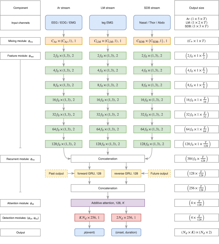
Figure 2: MSED network architecture. Left column contains component names, while right column shows the output dimensions for each operation as (number of filters[ x singleton] x time steps). Each stream in the middle (green) processes a separate set of input channels (blue, top), the results of which are concatenated before the bGRU (yellow). Outputs from the additive attention layer (purple) are convolved in the final classification and localization layers (red) to output the probabilities for each event class, and the predicted onset and duration of each event (blue, bottom). Convolution layers (orange, green, red) are detailed as [number of feature maps x kernel size, stride]. Recurrent layer (yellow) shows the direction and number of hidden units. Additive attention layer (purple) is described with the number of hidden and output units. GRU: gated recurrent unit; Ar: arousal; LM: leg movement; SDB: sleep disordered breathing.

Given an input set $\boldsymbol{\chi}=\left\{\mathbf{x},\boldsymbol{\varepsilon}^{t}\right\}\in\mathbb{R}^{C\times T}\times\mathbb{R}^{N_{t}\times 2}_{+}\times\mathcal{L}$ containing PSG data with $C$ channels and $T$ time steps, and true events $\boldsymbol{\varepsilon}$, the goal of the model is to detect any possible events in the segment, where, in this context, detection covers both classification and localization of any event in the segment space.

The model generates a set of default event windows $\boldsymbol{\varepsilon}^{d}=\left\{\varepsilon^{d}_{j}\mid j\in\left\llbracket N_{d}\right\rrbracket\right\}$ for the current segment, and matches each true event to a default event window if their intersection-over-union (IoU) is at least 0.5.

At test time, we generate predictions across the default event windows and use a non-maximum suppression procedure to select between the candidate predictions. For a given class k, the procedure is as follows: First, the predictions are sorted according to probability of the event, which is above a threshold $\theta_{k}$. Then, using the most probable prediction as an anchor, we sequentially evaluate the IoU between the anchor and the remaining candidate predictions, removing those with IoU larger than 0.5.

The output of the model is thus the set of predicted events $\boldsymbol{\varepsilon}^{p}=\left\{\mathbf{p},\mathbf{y}\right\}$ containing the predicted class probabilities along with the corresponding onsets and durations

3.3 Signal conditioning

We resampled all signals to a common sampling frequency of $f_{s}=$128\text{\,}\mathrm{Hz}$$ using a poly-phase filtering approach (Kaiser window, $\beta=$5.0$$). Based on recommended filter specifications from the AASM, we designed Butterworth IIR filters for four sets of signals [1]. EEG and EOG channels were filtered using a 2 order filter with a $0.3\text{\,}\mathrm{Hz}35\text{\,}\mathrm{Hz}$ passband, while chin and leg EMG channels were filtered using a 4 order high-pass filter with a $10\text{\,}\mathrm{Hz}$ cut-off frequency. Nasal pressure channels was filtered using a 4 order high-pass filter with a $0.03\text{\,}\mathrm{Hz}$ cut-off frequency, while thoracoabdominal channels were filtered using a 2 order filter with a $0.1\text{\,}\mathrm{Hz}15\text{\,}\mathrm{Hz}$ passband. All filters were implemented using the zero-phase method.

Filtered signals were subsequently standardized by subtracting signal means and dividing by signal standard deviations for each PSG.

3.4 Target encoding

For each data segment, target event classes $\boldsymbol{\pi}\in\mathbb{R}^{N_{m}\times K}$ were generated by one-hot encoding, and the target detection variable containing the onset and duration times $\mathbf{t}\in\mathbb{R}^{N_{m}\times 2}$ was encoded as

$$t_{i}=\left\lparen\frac{\varrho^{m}_{i}-\varrho^{d}_{j}}{\delta^{d}_{j}},\,\log\frac{\delta^{m}_{i}}{\delta^{d}_{j}}\right\rparen,\,i\in\left\llbracket N_{m}\right\rrbracket,\,j\in\left\llbracket N_{d}\right\rrbracket,$$ (1)

where $\varrho^{m}_{i}$ is the center point of the true event matched to a default event window $\varrho^{d}_{j}$, and $\delta^{m}_{i}$ and $\delta^{d}_{j}$ are the corresponding durations of the true and default events.

3.5 Data sampling

As the total number of default event windows $N_{d}$ in a data segment most likely will be much higher than the number of event windows matched to a true event, i. e. $N_{d}\gg N_{m}$, we implemented a similar random data sampling strategy as in [28]. At training step $t$, a given PSG record $r$ has a certain number of associated number of Ar, LM, and SDB events ($n_{\mathrm{Ar}},n_{\mathrm{LM}},n_{\mathrm{SDB}}$, respectively). We randomly sample a class $k$ with equal probability $p_{k}=\frac{1}{K-1}$, while disregarding the negative class since this is most likely over-represented in the data segment in any case. Given the class $k$, we randomly sample an event $\varepsilon_{k}$ from the PSG record $r$. We then randomly sample a $C\times T$ data segment with start time in the range $\left[\bar{\varepsilon}_{k}-T,\bar{\varepsilon}_{k}\right]$ where $\bar{\varepsilon}_{k}$ is the sample midpoint of the event $\varepsilon_{k}$. This ensures that a sampled data segment will contain at least $50\text{\,}\mathrm{\char 37\relax}$ of at least one event. We found that this approach to sampling data segments with a large ratio of negative to positive samples to be beneficial in all our experiments when monitoring the loss on the validation set.

3.6 Network architecture

Similar to the architecture described in [30], we designed a splitstream network architecture, where each stream is responsible for the bulk feature extraction for a specific event class. For the given problem of detecting Ars, LMs, and SDBs, the network contains three streams: the Ar stream takes as input the EEGs, the EOGs, and the chin EMG signals for a total of $C_{\text{Ar}}=5$ channels; the LM stream receives the $C_{\text{LM}}=2$ leg EMG signals; and the SDB stream receives the nasal pressure and the thoracoabdominal signals for a total of $C_{\text{SDB}}=3$ channels. An overview of the network architecture is shown graphically in Fig. 2.

3.6.1 Stream specifics

Each stream is comprised of two components. First, a mixing module $\varphi_{\text{mix}}:\mathbb{R}^{C_{\ast}\times T}\rightarrow\mathbb{R}^{C_{\ast}\times T}$ computes a non-linear mixing of the $C$ channels using a set of $C$ single-strided 1-dimensional filters $\mathbf{w}\in\mathbb{R}^{C\times C}$ and rectified linear unit (ReLU) activation [45]. Second, the output activations from $\varphi_{\text{mix}}$ are used as input to a feature extraction module $\varphi_{\text{feat}}:\mathbb{R}^{C_{\ast}\times T}\rightarrow\mathbb{R}^{f^{\prime}\times T^{\prime}}$, which transforms the input feature maps to a $f^{\prime}\times T^{\prime}$ feature space with a temporal dimension reduced by a factor of $\frac{T}{T^{\prime}}$. The feature extraction module $\varphi_{\text{feat}}$ is realized using $k_{\text{max}}$ successive convolutions with an increasing number of filters $f^{\prime}=f_{0}2^{k-1},\,k\in\llbracket k_{\text{max}}\rrbracket$, where $f_{0}$ is a tunable base filter number. Each feature map is normalized using batch normalization [46] with subsequent ReLU activation.

3.6.2 Feature fusion for sequential processing

The output vectors from each stream is concatenated into a combined feature vector $\mathbf{z}=\left\lparen\mathbf{z}_{\text{ar}},\mathbf{z}_{\text{lm}},\mathbf{z}_{\text{sdb}}\right\rparen\in\mathbb{R}^{3f^{\prime}\times T^{\prime}}$. We introduce sequential modeling of the feature vectors via a recurrent module $\varphi_{\text{rec}}:\mathbb{R}^{3f^{\prime}\times T^{\prime}}\rightarrow\mathbb{R}^{2n_{h}\times T^{\prime}}$ realized with a bidirectional gated recurrent unit (bGRU) [47]. The output of the bGRU for timestep t is a vector $\mathbf{h}_{t}=\left\lparen{\mathbf{h}_{t}^{\mathsf{f}}},{\mathbf{h}_{t}^{\mathsf{b}}}\right\rparen\in\mathbb{R}^{2n_{h}}$ containing the concatenated outputs from the forward (f) and backward (b) directions.

3.6.3 Additive attention

We implemented a simple additive attention mechanism [48], which computes context-vectors $\mathbf{c}\in\mathbb{R}^{2n_{h}\times K}$ for each event class as the weighted sum of the feature vector outputs $\mathbf{h}\in\mathbb{R}^{2n_{h}\times T^{\prime}}$ from the bGRU.

Formally, attention is computed as rCl c &= ∑_t^T^′ h_t α_t^⊺, where $\mathbf{h}_{t}$ is the feature vector for time step $t$, and $\boldsymbol{\alpha}_{t}\in\mathbb{R}^{K}$ is the attention weight computed as

$$\boldsymbol{\alpha}_{t}=\frac{\exp\left\lparen\mathbf{W}_{a}\tanh\left\lparen\mathbf{W}_{\text{u}}\mathbf{h}_{t}\right\rparen\right\rparen}{\sum_{\tau}^{T^{\prime}}\exp\left\lparen\mathbf{W}_{a}\tanh\left\lparen\mathbf{W}_{\text{u}}\mathbf{h}_{\tau}\right\rparen\right\rparen}.$$ (2)

Here, $\mathbf{W}_{u}\in\mathbb{R}^{n_{a}\times 2n_{h}}$ and $\mathbf{W}_{a}\in\mathbb{R}^{K\times n_{a}}$ are learnable linear mappings of the feature vectors.

3.6.4 Detection

The final event classification and localization is handled by two modules, $\psi_{\mathrm{clf}}:\mathbb{R}^{2n_{h}\times K}\to\mathbb{R}^{N_{d}\times K}$ and $\psi_{\mathrm{loc}}:\mathbb{R}^{2n_{h}\times K}\to\mathbb{R}^{N_{d}\times 2}$, respectively. The classification module $\psi_{\text{clf}}:\mathbf{c}\mapsto\mathbf{p}$ outputs a tensor $\mathbf{p}\in\left[0,1\right]^{N_{d}\times K}_{+}$ containing predicted event class probabilities for each default event window. The localization module $\psi_{\text{loc}}:\mathbf{c}\mapsto\mathbf{y}$ outputs a tensor $\mathbf{y}\in\mathbb{R}^{N_{d}\times 2}$ containing encoded relative onsets and durations for a detected event for each default event window.

3.7 Training objective

Similar to [37], we optimized the network parameters according to a three-component loss function consisting of i) a localization loss $\ell_{\mathrm{loc}}$ ii) a positive classification loss $\ell_{+}$ iii) a negative classification loss $\ell_{-}$ , such that the total loss $\ell$ was defined by

$$\ell=\ell_{\mathrm{loc}}+\ell_{+}+\ell_{-}.$$ (3)

The localization loss $\ell_{\mathrm{loc}}$ was calculated using a Huber function rCl ℓ_loc & = 1N+   ∑_i ∈π_+​f_H^(i),
f_H = {0.5 (y - t )2, if | y - t | < 1,| y - t | - 0.5, otherwise, where $i\in\pi_{+}$ yields indices of event windows with positive targets, i. e. event windows matched to an arousal, LM or SDB target, and $N_{+}$ is the number of positive targets in the given data segment.

The positive classification loss component $\ell_{+}$ was calculated using a simple cross-entropy over the event windows matched to an arousal, LM, or SDB event: rCl ℓ_+&=1N+   ∑_i ∈π_+ ∑_k ∈⟦K ⟧ π^(i)_k logp^(i)_k,
p^(i)_k=exps(i)k∑jexps(i)j, and $\pi^{(i)}_{k}$, $p^{(i)}_{k}$, and $s^{(i)}_{k}$ are the true class probability, predicted class probability, and logit score for the ith event window containing a positive sample.

Similar to [49, 36], the negative classification loss $\ell_{-}$ was calculated using a hard negative mining approach to balance the number of positive and negative samples in a data segment after matching default event windows to true events [50]. Specifically, this is accomplished by calculating the probability for the negative class (no event) for each unmatched default event window, and then calculating the cross entropy loss using the Z most probable samples. In our experiments, we set the ratio of positive to negative samples as 1:3, such that the calculation of $\ell$ involves $Z=3$ times as many negative as positive samples.

We also explored a focal loss objective function for computing $\ell_{+}$ and $\ell_{-}$ [51], however, we found that this approach severely deteriorated the ability of the network to accurately detect LM and SDB events compared to using worst negative mining.

3.8 Experimental setups

Table 2: MSED parameter settings.

Symbol	Description	Value
$n_{\text{train}}$	Number of train records	$1653$
$n_{\text{eval}}$	Number of eval records	$200$
$n_{\text{test}}$	Number of test records	$1000$
$C$	Number of input channels	$10$
$\delta$	Duration of default event windows	$3510\text{\,}\mathrm{s}$
$N_{d}$	Number of default event windows	$208$
$f_{s}$	Sampling rate	$128\text{\,}\mathrm{Hz}$
$T$	Segment length, samples	$15360$
$T^{\prime}$	Reduced segment length, samples	$120$
$k_{\mathrm{max}}$	Number of layers in $\varphi_{\mathrm{feat}}$	$7$
$f_{0}$	Base filter number	$4$
$f^{\prime}$	Feature vector size	$512$
$n_{h}$	Hidden units in bGRU	$128$
$n_{u}$	Hidden units in $\varphi_{\mathrm{att}}$	$128$
$K$	Number of output classes	$4$
$(\beta_{1},\beta_{2})$	Adam decay rates	$(0.9,0.999)$
$\eta$	Initial learning rate	$1\text{\times}{10}^{-3}$
	Learning rate decay factor	$0.1$
	Learning rate decay step	$3\text{ epochs}$
	Early stopping	$10\text{ epochs}$

In our experiments, we optimized the training objective using adaptive moment estimation (Adam) [52], according to the loss function described in Eq. 3. Exponential decay rates were fixed at $(\beta_{1},\beta_{2})=(0.9,0.999)$, the learning rate at $\eta=10^{-3}$, and $\epsilon=10^{-8}$. The learning rate was decayed in a step-wise manner by multiplying $\eta$ with a factor of 0.1 after 3 consecutive epochs with no improvement in loss value on the validation dataset. Similarly, we employed an early stopping scheme by monitoring the loss on the validation dataset and stopping the model training after 10 epochs of no improvement on $\mathcal{D}_{\textsc{eval}}$.

We tested four types of models in two categories: the first is a default split-stream model as shown in Fig. 2 with and without weight decay (splitstream, splitstream-wd). The second is a variation of the split-stream model, but where the $\psi_{\text{clf}}$ and $\psi_{\text{loc}}$ modules are realized using depth-wise convolutions, such that each attention group is used only for that type of event. The second category is also tested with and without weight decay (splitstream-dw, splitstream-dw-wd).

We benchmarked our proposed MSED model against DOSED by comparing overall performance on $\mathcal{D}_{\text{test}}$ after training on $n_{\text{train}}=200$ subject PSGs. Each model was allowed 100 epochs of training, and the optimal models were selected based on lowest loss score on $\mathcal{D}_{\text{eval}}$ across epochs. F1, precision, and recall scores were obtained by evaluating optimized models on $\mathcal{D}_{\text{test}}$.

Various model parameters are shown in Table 2.

3.9 Performance evaluation

Performance was quantified using precision, recall, and F1 scores. Statistical significance in F1 score between groups was assessed with Kruskall-Wallis H-tests. The performance of joint vs. single-event detection models was tested with Wilcoxon signed rank tests for matched samples. The relationships between true and predicted arousal index (ArI), AHI, and LMI were assessed using linear models and Pearson’s $r^{2}$. Significance was set at $\alpha=0.05$.

4 Results and discussion

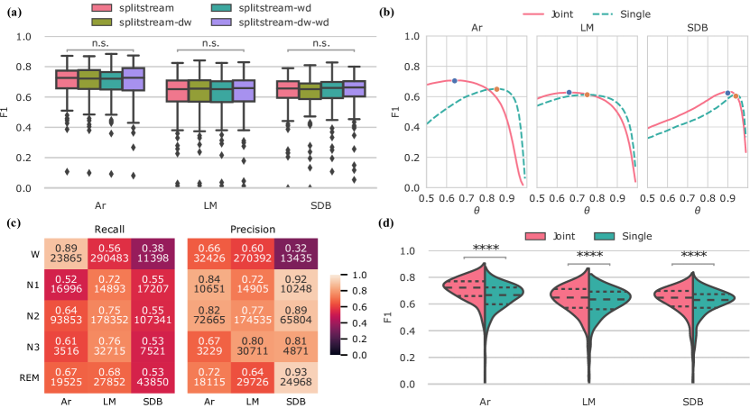
Figure 3: Optimizing MSED architecture and model evaluation. (a) No significant differences in F1 were found between model architectures. (b) Optimizing F1 performance on $\mathcal{D}_{\text{eval}}$ as a function of detection threshold $\theta$ for joint (solid) and single-event (dashed) detection models. Blue and orange dots correspond to optimal $\theta$/F1 pair. (c) Analysing event recall and precision categorized by sleep stage origin on $\mathcal{D}_{\text{test}}$ data. E.g. out of 19525 Ar events manually scored in REM, the optimal model correctly identifies 0.67%, while out of 10248 SDB events predicted in N1, 0.92% of these are also manually scored. (d) Evaluating optimized joint and single-event detection models on $\mathcal{D}_{\text{test}}$ given the respective detection threshold $\theta$ from (b). For all three event types, the joint detection model outperforms the single-event models based on F1. Dashed lines in the violin plot interior show the associated 25, 50, and 75 percentiles. ^∗∗∗∗: $p<0.001$. W: wakefulness; N1: non- stage 1; N2: non- stage 2; N3: non- stage 3; REM: rapid eye movement; Ar: arousal; LM: leg movement; SDB: sleep disordered breathing.

Table 3: Temporal difference metrics across event types and PSGs for joint and single prediction models. Positive values of onset/offset correspond to delayed predictions relative to the matched true event, while positive duration values correspond to an overestimation of event duration. Metrics are shown as mean ± standard deviation with 95% confidence interval in brackets across all events for all PSG recordings.

		duration	onset	offset
Ar	Joint	$4.81\pm 2.92$ $[1.07,10.77]$	$-1.37\pm 1.39$ $[-3.99,0.33]$	$3.44\pm 2.24$ $[0.56,7.41]$
	Single	$6.42\pm 3.70$ $[1.37,12.99]$	$-1.94\pm 1.93$ $[-5.33,0.50]$	$4.49\pm 2.69$ $[0.85,9.21]$
LM	Joint	$-0.46\pm 0.36$ $[-1.05,0.07]$	$0.24\pm 0.22$ $[-0.04,0.56]$	$-0.23\pm 0.20$ $[-0.55,0.05]$
	Single	$-0.51\pm 0.39$ $[-1.16,0.01]$	$0.26\pm 0.23$ $[-0.02,0.61]$	$-0.25\pm 0.21$ $[-0.61,0.06]$
SDB	Joint	$20.41\pm 13.36$ $[3.50,43.77]$	$-9.39\pm 6.74$ $[-21.24,-0.97]$	$11.02\pm 7.67$ $[1.14,23.70]$
	Single	$34.95\pm 16.63$ $[10.81,63.18]$	$-16.00\pm 8.80$ $[-32.35,-3.65]$	$18.95\pm 9.51$ $[5.44,35.33]$

• Ar: arousal; LM: leg movement; SDB: sleep disordered breathing.

4.1 Model architecture evaluation

We found no significant differences in F1 performance for either Ar (Kruskal-Wallis $H=0.96,\,p=0.81$), LM ($H=0.23,\,p=0.97$), or SDB detection ($H=2.84,\,p=0.42$), when evaluating the model architectures on $\mathcal{D}_{\text{eval}}$ (see Fig. 3a). Subsequent results are thus reported based on the default splitstream architecture.

4.2 Optimizing threshold for joint vs. single event detection

Table 4: Performance scores for optimized models evaluated on $\mathcal{D}_{\text{test}}$. Metrics are shown aggregated across PSGs as mean ± standard deviation. Overall metrics are computed by averaging scores for each subject PSG.

		Joint	Single
Ar	F1	$0.704\pm 0.106$	$0.649\pm 0.113$
	Pr	$0.759\pm 0.114$	$0.777\pm 0.107$
	Re	$0.672\pm 0.125$	$0.571\pm 0.127$
LM	F1	$0.628\pm 0.123$	$0.613\pm 0.116$
	Pr	$0.650\pm 0.169$	$0.661\pm 0.166$
	Re	$0.647\pm 0.120$	$0.607\pm 0.116$
SDB	F1	$0.624\pm 0.115$	$0.604\pm 0.118$
	Pr	$0.817\pm 0.142$	$0.835\pm 0.136$
	Re	$0.526\pm 0.146$	$0.492\pm 0.145$
Overall	F1	$0.652\pm 0.121$	$0.622\pm 0.117$
	Pr	$0.742\pm 0.159$	$0.758\pm 0.157$
	Re	$0.615\pm 0.146$	$0.556\pm 0.138$

• Ar: arousal; LM: leg movement; SDB: sleep disordered breathing; Pr: precision; Re: recall.

For each event type, we evaluated the F1 score as a function of classification threshold $\theta$ on $\mathcal{D}_{\text{eval}}$ for both the joint detection model as well as the single-event models. It can be observed in Fig. 3b that for all three events, the joint detection model achieves higher F1 score, although the increase is not as large for LM and SDB detection. This was also observed when evaluating the joint and single detection models with optimized thresholds on $\mathcal{D}_{\text{test}}$ for both Ar (Wilcoxon $W=30440,\,p<0.001$), LM ($W=101103,\,p<0.001$), and SDB detection ($W=125461,\,p<0.001$), see Fig. 3d. Precision, recall and F1 scores for optimized models evaluated on are shown in Table 4. These findings provide evidence that the presence of certain event types can modulate the detection of other event types, and that this can be modeled using automatic methods. This is in line with what previous studies have found e. g. on event-by-event scoring agreement in arousals, which improved significantly from $58.7\text{\,}\mathrm{\char 37\relax}90.5\text{\,}\mathrm{\char 37\relax}$, when including respiratory signals in the analysis [17].

4.3 Comparison with state-of-the-art multi-event detection

F1, recall, and precision scores for optimized DOSED and MSED models evaluated on $\mathcal{D}_{\text{test}}$ are shown in Table 5. We observed an overall MSED F1 score of 0.634 ± 0.124 against an overall DOSED F1 score of 0.596 ± 0.140; and overall F1 scores for Ar, LM, and SDB of 0.677 ± 0.107, 0.599 ± 0.127, and 0.626 ± 0.125 for MSED, and 0.668 ± 0.115, 0.619 ± 0.125, and 0.503 ± 0.123 for DOSED. Factoring in the overall reduction in model size from 385,489,502 to 9,435,606 parameters, these results show the advantage of MSED compared to DOSED on the same dataset.

Comparing with existing single-event arousal detection models, MSED does not perform on the level of previous state-of-the-art proposed by [30] [30]. Here, an EEG+EOG+EMG combination model for combined sleep-wake classification and arousal detection yielded an F1 score of 0.76, although this was reported on a much smaller dataset. Similarly, in the work by [31], a model combining two leg EMG channels achieved an impressive F1 score of 0.77 [31], although this was also reported in a much smaller dataset. We did not perform in-depth ablations in this study, so it is possible that the MSED performance could be higher given sufficient fine-tuning. However, it is also worth noting that both of these models apply post-processing of the model outputs, most notably the removal of arousals and leg movements scored in wake, which is not performed in the current work, and fusion of events within certain manually-set thresholds. It is possible that this approach introduces a negative bias in our proposed model, since it is evident from Fig. 3c that the precision for all scored events is lower in W than in other sleep stages. In this work we wished the predictions to be orthogonal to manual sleep scoring, but future work should consider adding an automatic sleep scoring module to the model architecture.

While literature on sleep apnea detection is extensive, it is difficult to compare directly to the proposed approach, because the majority of studies either focus on obstructive apnea alone, do not report F1, precision, or recall scores, or only focus on the prediction of AHI alone [53].

However, one recent study compared the event-by-event detection performance against a concensus score of five technicians. They reported an average human performance quantified by F1 of 0.55, and an F1 score from the automatic method of 0.57 [54] Similarly, [55] recently proposed their WaveNet model for precisely annotating SDB events in 1 s bins. Although their model also included post-processing of the bins, they obtained a mean F1 score across events of 0.406. We therefore see a marked improvement from the state of the art event detectors compared to MSED.

These results also indicate the massive research potential in terms of other ways to assess SDB; apart from AHI, which is an average across the entire night, researchers and clinicians could potentially benefit from taking a more fine-grained approach. As illustrated by [56], patients with the exact same AHI can exhibit wildly different activity patterns (breathing disturbances) [56], yet this is unaccounted for in state-of-the-art apnea detection models, as the majority of these are epoch-based [53]. [56] proposes "instantaneous AHI" as a solution to this problem, although their results were based on human annotation and not automatic detection as proposed here. The integration of these two methods would be an interesting approach for future research.

In addition, future work should explore novel methods for object detection in the computer vision literature. Most notably, the use of default event windows impose certain restrictions on the temporal scale of detected events, and this could be eliminated by using a Transformer-based detection model, such as the one found in the Detection Transformer [57]. Here, predictions are generated using a number of object queries, which are independent from the default event windows and thus not restricting the temporal scale of the events.

Table 5: Comparing model performance against DOSED on a reduced $\mathcal{D}_{\text{train}}$. Metrics are shown aggregated across PSGs as mean ± standard deviation. Overall metrics are computed by averaging scores for each subject PSG.

		DOSED	MSED
Ar	F1	$0.668\pm 0.115$	$0.677\pm 0.107$
	Pr	$0.711\pm 0.120$	$0.688\pm 0.118$
	Re	$0.651\pm 0.141$	$0.686\pm 0.131$
LM	F1	$0.619\pm 0.125$	$0.599\pm 0.127$
	PR	$0.634\pm 0.169$	$0.655\pm 0.174$
	Re	$0.644\pm 0.120$	$0.587\pm 0.133$
SDB	F1	$0.503\pm 0.123$	$0.626\pm 0.125$
	Pr	$0.706\pm 0.173$	$0.793\pm 0.146$
	Re	$0.412\pm 0.133$	$0.542\pm 0.157$
Overall	F1	$0.596\pm 0.140$	$0.634\pm 0.124$
	Pr	$0.684\pm 0.160$	$0.712\pm 0.159$
	Re	$0.568\pm 0.172$	$0.605\pm 0.153$
No. parameters		385,489,502	9,435,606

• Ar: arousal; LM: leg movement; SDB: sleep disordered breathing; Pr: precision; Re: recall.

4.4 Correlation between experts and model

For each event type, we computed the correlation coefficient between predicted and expert-annotated ArI, AHI, and LMI, which is shown in Fig. 4. We found a large positive correlation between true and predicted values for ArI ($r^{2}=0.73$, $p<0.001$), AHI ($r^{2}=0.77$, $p<0.001$), and LMI ($r^{2}=0.78$, $p<0.001$).

A similar study by [24] using an automatic method for automatic detection of SDB and LM events found similar or higher correlations between automatic and manual scoring ($r^{2}_{\mathrm{SDB}}=0.85$, and $r^{2}_{\mathrm{LM}}=0.79$, respectively), although their findings were based on almost 5 times as much data [24]. Furthermore, obstructive, central, mixed and hypopneas with an associated 4% desaturation were lumped together into a single apnea class, which may have introduced unwanted bias towards obstructive apneas and hypopneas in their findings, since these are in general more prevalent than central and mixed apneas.

4.5 Temporal difference metrics

We compared the temporal precision between manual and MSED event scoring by looking at the errors in onset ($\Delta\text{onset}$), offsets ($\Delta\text{fffset}$), and durations ($\Delta\text{duration}$) calculated as

$$\Delta\,\text{onset} =\text{onset}_{\text{MSED}}-\text{onset}_{\text{manual}}$$ (4)

$$\Delta\,\text{offset} =\text{offset}_{\text{MSED}}-\text{offset}_{\text{manual}}$$ (5)

$$\Delta\,\text{duration} =\text{duration}_{\text{MSED}}-\text{duration}_{\text{manual}}$$ (6)

so that positive values of $\Delta\,\text{onset},\Delta\,\text{offset}$ corresponds to a positive shift to the right (delayed prediction), and positive values of $\Delta\,\text{duration}$ meaning an overestimation of the event duration compared to manual scoring.

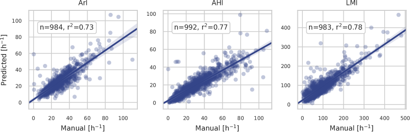
Figure 4: Pearson correlation plots for each event type index between true and predicted values. The linear relationship is indicated with solid blue with 95% confidence intervals in light blue. ArI: arousal index; AHI: apnea-hypopnea index; LMI: leg movement index.

Described in Table 3, the model overestimates the duration of Ar events by a couple of seconds, which is caused by an earlier prediction of onset and delayed prediction of termination. For LM events, the model underestimates the duration by about half a second on average, which is due to earlier prediction of termination. For SDB events, the model overestimates the duration by about 25 seconds on average, which is caused by an earlier prediction of onset and delayed prediction of termination. These errors in predicted duration reflect the temporal characteristics of these events; LMs are shorter events (between $0.5\text{\,}\mathrm{s}10\text{\,}\mathrm{s}$ per definition), and it is thus unlikely to be overestimated by several seconds, while SDBs are longer events by one to two orders of magnitude, which also increases the size of the errors. Arousals are intermediate in length compared to LMs and SDBs, which is reflected in the error distributions.

5 Conclusion

We have presented a novel method for detecting short and long events present in polysomnogram recordings based on deep neural networks. Our method was able to distinguish between arousals, limb movements, and sleep-disordered breathing events with F1 scores of 0.70, 0.63, and 0.62, respectively, and we furthermore found that jointly optimizing a model for all three events performed better than the respective models optimized for each specific event type.

We benchmarked our algorithm against previous state-of-the-art and report an overall increase in F1 score from 0.60 to 0.63 despite a 97.5% reduction in memory footprint.

Furthermore, clinically relevant derivatives (ArI, AHI, LMI) showed a high positive correlation with manually computed values indicating a high degree of agreement between our model and experts.

Future work should incorporate ides from the object detection in computer vision literature and investigate more complex models with increased flexibility towards adding prediction capabilities for additional event types. Additionally, the low precision across all events observed during wakefulness could be remedied by incorporating an automatic sleep stage classification model which also merits further investigation.

References

- [1] Richard B. Berry et al. “The AASM Manual for the Scoring of Sleep and Associated Events: Rules, Terminology and Technical Specifications, Version 2.6” Darien, IL, USA: American Academy of Sleep Medicine, 2020
- [2] Péter Halász et al. “The nature of arousal in sleep” In J. Sleep Res. 13.1, 2004, pp. 1–23 DOI: 10.1111/j.1365-2869.2004.00388.x
- [3] R. Ferri et al. “World Association of Sleep Medicine (WASM) 2016 standards for recording and scoring leg movements in polysomnograms developed by a joint task force from the International and the European Restless Legs Syndrome Study Groups (IRLSSG and EURLSSG)” In Sleep Med. 26, 2016, pp. 86–95 DOI: 10.1016/j.sleep.2016.10.010
- [4] Raffaele Ferri et al. “Periodic leg movements during sleep: phenotype, neurophysiology, and clinical significance” In Sleep Med. 31, 2017, pp. 29–38 DOI: 10.1016/j.sleep.2016.05.014
- [5] Richard S Rosenberg and Steven Van Hout “The American Academy of Sleep Medicine Inter-scorer Reliability Program: Respiratory Events” In J. Clin. Sleep Med. 10.4, 2014, pp. 447–454 DOI: 10.5664/jcsm.3630
- [6] Robert G Norman et al. “Interobserver Agreement Among Sleep Scorers From Different Centers in a Large Dataset” In Sleep 23.7, 2000, pp. 1–8 DOI: 10.1093/sleep/23.7.1e
- [7] Heidi Danker-Hopfe et al. “Interrater reliability between scorers from eight European sleep laboratories in subjects with different sleep disorders” In J. Sleep Res. 13, 2004, pp. 63–69 DOI: 10.1046/j.1365-2869.2003.00375.x
- [8] Heidi Danker-Hopfe et al. “Interrater reliability for sleep scoring according to the Rechtschaffen & Kales and the new AASM standard” In J. Sleep Res. 18.1, 2009, pp. 74–84 DOI: 10.1111/j.1365-2869.2008.00700.x
- [9] Richard S. Rosenberg and Steven Van Hout “The American Academy of Sleep Medicine Inter-scorer Reliability Program: Sleep Stage Scoring” In J. Clin. Sleep Med. 9, 2013, pp. 81–87 DOI: 10.5664/jcsm.2350
- [10] Xiaozhe Zhang et al. “Process and outcome for international reliability in sleep scoring” In Sleep Breath. 19.1, 2015, pp. 191–195 DOI: 10.1007/s11325-014-0990-0
- [11] Magdy Younes, Jill Raneri and Patrick Hanly “Staging sleep in polysomnograms: Analysis of inter-scorer variability” In J. Clin. Sleep Med. 12.6, 2016, pp. 885–894 DOI: 10.5664/jcsm.5894
- [12] Magdy Younes et al. “Reliability of the American Academy of Sleep Medicine Rules for Assessing Sleep Depth in Clinical Practice” In J. Clin. Sleep Med. 14.2, 2018, pp. 205–213 DOI: 10.5664/jcsm.6934
- [13] Michael J Drinnan et al. “Interobserver Variability in Recognizing Arousal in Respiratory Sleep Disorders” In Am. J. Respir. Crit. Care Med. 158, 1998, pp. 358–362 DOI: 10.1164/ajrccm.158.2.9705035
- [14] Coralyn W. Whitney et al. “Reliability of scoring respiratory disturbance indices and sleep staging” In Sleep 21.7, 1998, pp. 749–757 DOI: 10.1093/sleep/21.7.749
- [15] José S. Loredo et al. “Night-to-Night Arousal Variability and Interscorer Reliability of Arousal Measurements” In Sleep 22.7, 1999, pp. 916–920 DOI: 10.1093/sleep/22.7.916
- [16] M.V. Smurra et al. “Sleep fragmentation: comparison of two definitions of short arousals during sleep in OSAS patients” In Eur. Respir. J. 17, 2001, pp. 723–727 DOI: 10.1183/09031936.01.17407230
- [17] Robert Joseph Thomas “Arousals in Sleep-disordered Breathing: Patterns and Implications” In Sleep 26.8, 2003, pp. 1042–1047 DOI: 10.1093/sleep/26.8.1042
- [18] Michael H. Bonnet et al. “The scoring of arousal in sleep: Reliability, validity, and alternatives” In J. Clin. Sleep Med. 3.2, 2007, pp. 133–145 DOI: 10.5664/jcsm.26815
- [19] Ulysses J. Magalang et al. “Agreement in the Scoring of Respiratory Events and Sleep Among International Sleep Centers” In Sleep 36.4, 2013, pp. 591–596 DOI: 10.5665/sleep.2552
- [20] Henriette Koch et al. “Automatic sleep classification using a data-driven topic model reveals latent sleep states” In J. Neurosci. Methods 235, 2014, pp. 130–137 DOI: 10.1016/j.jneumeth.2014.07.002
- [21] Akara Supratak et al. “DeepSleepNet: A Model for Automatic Sleep Stage Scoring Based on Raw Single-Channel EEG” In IEEE Trans. Neural Syst. Rehabil. Eng. 25.11, 2017, pp. 1998–2008 DOI: 10.1109/TNSRE.2017.2721116
- [22] Stanislas Chambon et al. “A Deep Learning Architecture for Temporal Sleep Stage Classification Using Multivariate and Multimodal Time Series” In IEEE Trans. Neural Syst. Rehabil. Eng. 26.4, 2018, pp. 758–769 DOI: 10.1109/TNSRE.2018.2813138
- [23] Alexander Neergaard Olesen et al. “Deep residual networks for automatic sleep stage classification of raw polysomnographic waveforms” In 2018 40th Annu. Int. Conf. IEEE Eng. Med. Biol. Soc. Honolulu, HI, USA: IEEE, 2018, pp. 1–4 DOI: 10.1109/EMBC.2018.8513080
- [24] Siddharth Biswal et al. “Expert-level sleep scoring with deep neural networks” In J. Am. Med. Informatics Assoc. 25.12, 2018, pp. 1643–1650 DOI: 10.1093/jamia/ocy131
- [25] Jens B Stephansen et al. “Neural network analysis of sleep stages enables efficient diagnosis of narcolepsy” In Nat. Commun. 9.1, 2018, pp. 5229 DOI: 10.1038/s41467-018-07229-3
- [26] Huy Phan et al. “Joint Classification and Prediction CNN Framework for Automatic Sleep Stage Classification” In IEEE Trans. Biomed. Eng. 66.5, 2019, pp. 1285–1296 DOI: 10.1109/TBME.2018.2872652
- [27] Huy Phan et al. “SeqSleepNet: End-to-End Hierarchical Recurrent Neural Network for Sequence-to-Sequence Automatic Sleep Staging” In IEEE Trans. Neural Syst. Rehabil. Eng. 27.3, 2019, pp. 400–410 DOI: 10.1109/TNSRE.2019.2896659
- [28] Alexander Neergaard Olesen et al. “Towards a Flexible Deep Learning Method for Automatic Detection of Clinically Relevant Multi-Modal Events in the Polysomnogram” In 2019 41st Annu. Int. Conf. IEEE Eng. Med. Biol. Soc. Berlin, Germany: IEEE, 2019, pp. 556–561 DOI: 10.1109/EMBC.2019.8856570
- [29] Diego Alvarez-Estevez and Isaac Fernández-Varela “Large-scale validation of an automatic EEG arousal detection algorithm using different heterogeneous databases” In Sleep Med. 57, 2019, pp. 6–14 DOI: 10.1016/j.sleep.2019.01.025
- [30] Andreas Brink-Kjaer et al. “Automatic detection of cortical arousals in sleep and their contribution to daytime sleepiness” In Clin. Neurophysiol. 131.6, 2020, pp. 1187–1203 DOI: 10.1016/j.clinph.2020.02.027
- [31] Lorenzo Carvelli et al. “Design of a deep learning model for automatic scoring of periodic and non-periodic leg movements during sleep validated against multiple human experts” In Sleep Med. 69, 2020, pp. 109–119 DOI: 10.1016/j.sleep.2019.12.032
- [32] Mohammad Ghassemi et al. “You Snooze, You Win: The PhysioNet/Computing in Cardiology Challenge 2018” In 2018 Computing in Cardiology Conference (CinC) 45 IEEE, 2018, pp. 1–4 DOI: 10.22489/CinC.2018.049
- [33] Ary L. Goldberger et al. “PhysioBank, PhysioToolkit, and PhysioNet: Components of a new research resource for complex physiologic signals” In Circulation 101.23, 2000, pp. e215–e220 DOI: 10.1161/01.CIR.101.23.e215
- [34] Andreas Brink-Kjaer et al. “Cortical arousal frequency is increased in narcolepsy type 1” In Sleep 44.5, 2021, pp. zsaa255 DOI: 10.1093/sleep/zsaa255
- [35] Andreas Brink-Kjær et al. “Arousal characteristics in patients with Parkinson’s disease and isolated rapid eye movement sleep behavior disorder” In Sleep 44.12, 2021, pp. zsab167 DOI: 10.1093/sleep/zsab167
- [36] S. Chambon et al. “DOSED: A deep learning approach to detect multiple sleep micro-events in EEG signal” In J. Neurosci. Methods 321, 2019, pp. 64–78 DOI: 10.1016/j.jneumeth.2019.03.017
- [37] Alexander Neergaard Olesen et al. “Deep transfer learning for improving single-EEG arousal detection” In 2020 42nd Annu. Int. Conf. IEEE Eng. Med. Biol. Soc. Montreal, QC, Canada: IEEE, 2020, pp. 99–103 DOI: 10.1109/EMBC44109.2020.9176723
- [38] Janet Babich Blank et al. “Overview of recruitment for the osteoporotic fractures in men study (MrOS)” In Contemp. Clin. Trials 26.5, 2005, pp. 557–568 DOI: 10.1016/j.cct.2005.05.005
- [39] Eric Orwoll et al. “Design and baseline characteristics of the osteoporotic fractures in men (MrOS) study — A large observational study of the determinants of fracture in older men” In Contemp. Clin. Trials 26.5, 2005, pp. 569–585 DOI: 10.1016/j.cct.2005.05.006
- [40] Terri Blackwell et al. “Associations Between Sleep Architecture and Sleep-Disordered Breathing and Cognition in Older Community-Dwelling Men: The Osteoporotic Fractures in Men Sleep Study” In J. Am. Geriatr. Soc. 59.12, 2011, pp. 2217–2225 DOI: 10.1111/j.1532-5415.2011.03731.x
- [41] American Sleep Disorders Association “EEG arousals: scoring rules and examples: a preliminary report from the Sleep Disorders Atlas Task Force of the American Sleep Disorders Association” In Sleep 15.2, 1992, pp. 173–184
- [42] Marco Zucconi et al. “The official World Association of Sleep Medicine (WASM) standards for recording and scoring periodic leg movements in sleep (PLMS) and wakefulness (PLMW) developed in collaboration with a task force from the International Restless Legs Syndrome Study Group” In Sleep Med. 7.2, 2006, pp. 175–183 DOI: 10.1016/j.sleep.2006.01.001
- [43] Dennis A. Dean et al. “Scaling Up Scientific Discovery in Sleep Medicine: The National Sleep Research Resource” In Sleep 39.5, 2016, pp. 1151–1164 DOI: 10.5665/sleep.5774
- [44] Guo-Qiang Zhang et al. “The National Sleep Research Resource: towards a sleep data commons” In J. Am. Med. Informatics Assoc. 25.10, 2018, pp. 1351–1358 DOI: 10.1093/jamia/ocy064
- [45] Vinod Nair and Geoffrey E. Hinton “Rectified Linear Units Improve Restricted Boltzmann Machines” In Proc. 27th Int. Conf. Mach. Learn. (ICML), 2010 URL: https://icml.cc/Conferences/2010/papers/432.pdf
- [46] Sergey Ioffe and Christian Szegedy “Batch Normalization: Accelerating Deep Network Training by Reducing Internal Covariate Shift” In Proc. 32nd Int. Conf. Mach. Learn. Lille, France: JMLR, 2015 arXiv:1502.03167 [cs.LG]
- [47] Kyunghyun Cho et al. “On the Properties of Neural Machine Translation: Encoder–Decoder Approaches” In Proc. SSST-8, Eighth Work. Syntax. Semant. Struct. Stat. Transl. Stroudsburg, PA, USA: Association for Computational Linguistics, 2014, pp. 103–111 DOI: 10.3115/v1/W14-4012
- [48] Dzmitry Bahdanau, Kyunghyun Cho and Yoshua Bengio “Neural Machine Translation by Jointly Learning to Align and Translate” In 3rd Int. Conf. Learn. Represent. (ICLR 2015), 2015 arXiv:1409.0473 [cs.CL]
- [49] Stanislas Chambon et al. “A Deep Learning Architecture to Detect Events in EEG Signals During Sleep” In 2018 IEEE 28th Int. Work. Mach. Learn. Signal Process. Aalborg, Denmark: IEEE, 2018, pp. 1–6 DOI: 10.1109/MLSP.2018.8517067
- [50] Wei Liu et al. “SSD: Single Shot MultiBox Detector” In Comput. Vis. – ECCV 2016 Cham, Switzerland: Springer, 2016, pp. 21–37 DOI: 10.1007/978-3-319-46448-0_2
- [51] Tsung-Yi Lin et al. “Focal Loss for Dense Object Detection” In IEEE Trans. Pattern Anal. Mach. Intell. 42.2, 2020, pp. 318–327 DOI: 10.1109/TPAMI.2018.2858826
- [52] Diederik P Kingma and Jimmy Ba “Adam: A Method for Stochastic Optimization”, 2014 arXiv:1412.6980 [cs.LG]
- [53] Fábio Mendonça et al. “A Review of Obstructive Sleep Apnea Detection Approaches” In IEEE Journal of Biomedical and Health Informatics 23.2, 2019, pp. 825–837 DOI: 10.1109/JBHI.2018.2823265
- [54] Valentin Thorey et al. “AI vs Humans for the Diagnosis of Sleep Apnea” In 2019 41st Annu. Int. Conf. IEEE Eng. Med. Biol. Soc. EMBC Berlin, Germany: IEEE, 2019, pp. 1596–1600 DOI: 10.1109/EMBC.2019.8856877
- [55] Thijs E. Nassi et al. “Automated Scoring of Respiratory Events in Sleep With a Single Effort Belt and Deep Neural Networks” In IEEE Trans. Biomed. Eng. 69.6, 2022, pp. 2094–2104 DOI: 10.1109/TBME.2021.3136753
- [56] Shuqiang Chen et al. “Dynamic Models of Obstructive Sleep Apnea Provide Robust Prediction of Respiratory Event Timing and a Statistical Framework for Phenotype Exploration” In Sleep 45.12, 2022, pp. zsac189 DOI: 10.1093/sleep/zsac189
- [57] Nicolas Carion et al. “End-to-End Object Detection with Transformers” Series Title: Lecture Notes in Computer Science In Computer Vision – ECCV 2020 12346 Cham: Springer International Publishing, 2020, pp. 213–229 DOI: 10.1007/978-3-030-58452-8_13