Locally supported, quasi-interpolatory bases on graphs

Abstract

Lagrange functions are localized bases that have many applications in signal processing and data approximation. Their structure and fast decay make them excellent tools for constructing approximations. Here, we propose perturbations of Lagrange functions on graphs that maintain the nice properties of Lagrange functions while also having the added benefit of being locally supported. Moreover, their local construction means that they can be computed in parallel, and they are easily implemented via quasi-interpolation.

1 Introduction

In our previous paper, we considered Lagrange functions on graphs, proving exponential decay properties of the functions themselves as well as the coefficients in an approximation [18]. While they have many nice features, one issue with using full Lagrange functions is that they are globally supported. This means that when new data is acquired, all of the Lagrange functions must be recomputed to form a new approximation, and their fast decay means that we are storing many very small values unnecessarily. The latter problem could be addressed by truncating the functions outside of a specified footprint; however, we would still need to compute the full Lagrange functions first. Instead we propose local Lagrange functions that are computed using only the values close to their centers as well as setting the values outside of a local footprint to zero. This approach addresses both concerns. Moreover, we show that these proposed functions can be made arbitrarily close to the full Lagrange functions so that we do not lose any of the previously derived positive attributes.

In addition to the nice properties mentioned above, there are others. Locally supported bases allow us to use sparse data formats to save in storage. Being locally constructed, we can compute the Local Lagrange bases in parallel. When new data is acquired, only the local Lagrange functions close to the new data have to be updated.

The bases that we consider are connected to the early work on kernels and splines on graphs [16] as well as the analysis of variational splines on graphs [11, 12, 13]. More recently, splines and wavelets on circulant graphs were studied in [10]. Positive definite basis functions on graphs were considered for machine learning in [5, 6]. Dictionaries of functions on graphs were treated in [14]. A variety of signal processing techniques on graphs are also closely related [15, 3, 9].

Our approach to local Lagrange bases is rooted in the continuous domain theory [7, 8], but it differs in a few ways, primarily due the differences in the Greens functions. On a continuous domain, the Greens functions are readily available with user-friendly formulas. On a graph, the Greens functions are costly to compute as the pseudo-inverse of a large matrix. Therefore, in the graph setting, we use energy minimization to compute the local Lagrange functions.

1.1 Setting

As in [18], we consider a finite, connected, weighted graph $\mathcal{G}=\left\{\mathcal{V},\mathbf{E}\subset\mathcal{V}\times\mathcal{V},w,\rho\right\}$. The vertex set is $\mathcal{V}$. The edge set is $\mathbf{E}$.

The function $\rho:\mathcal{V}\times\mathcal{V}\rightarrow\mathbb{R}_{\geq 0}$ is a distance function on the graph. We require $\rho$ to be positive on distinct pairs of vertices. We denote the maximum distance between adjacent vertices as $\rho_{\text{max}}$. Given the distance between adjacent vertices, the distance between non-adjacent vertices is the length of the shortest path connecting them.

The weight function $w:\mathcal{V}\times\mathcal{V}\rightarrow\mathbb{R}_{\geq 0}$ is assumed to be symmetric. In this paper, we set the weight of an edge to be the inverse of the length of the edge (specified by $\rho$). The $i,j$ entry of the adjacency matrix $A$ is the weight of the edge connecting the corresponding vertices. If no edge connects the vertices, the entry is 0.

We assume $\mathcal{G}$ has at least two vertices. We denote the maximum degree of the vertices in the graph by $M\in\mathbb{Z}_{\geq 1}$.

The $j$th diagonal entry of the diagonal matrix $D$ is equal to the $j$th row sum of $A$. The normalized graph Laplacian is $L=D^{-1/2}(D-A)D^{-1/2}$ [1, 2]. The entries of the normalized Laplacian are bounded by 1, and the diagonal entries are exactly 1.

1.2 Notation

The Lagrange function centered at vertex $v$ will be denoted as $\chi_{v}$, $\chi(\cdot,v)$, or just $\chi$ when specifying the center is unnecessary. The local Lagrange function centered at vertex $v$ will be denoted $\bar{\chi}_{v}$, $\bar{\chi}(\cdot,v)$, or $\bar{\chi}$.

We shall use the subscripts $k$ and $u$ to denote vertices where data is known and unknown, respectively. For example $\mathcal{V}_{k}$ will represent the set of all vertices where data is known.

A neighborhood of a vertex $v$ is denoted $\Omega_{v}$. The neighborhoods $\Omega_{v}$ will be chosen to satisfy Dirichlet boundary conditions, i.e. the boundary vertices are in $\mathcal{V}_{k}$. The radius $R_{v}$ of a neighborhood $\Omega_{v}$ will factor into the error between the Lagrange and local Lagrange bases. The maximum number of nodes over all such neighborhoods is denoted $N_{\Omega}$.

The Lagrange function $\chi_{v}$ restricted to the known vertices will be denoted $\chi_{v,k}$. Similarly, $\chi_{v,u}$ denotes $\chi_{v}$ restricted to the unknown vertices.

When a set is used as a subscript for the Laplacian, we mean the submatrix determined by the rows and columns of the set, e.g. $L_{\Omega_{v}}$ denotes the Laplacian restricted to the neighborhood $\Omega_{v}$

The submatrix of the Laplacian corresponding to the columns of unknown vertices is denoted $L_{u}$, and $L_{k}$ denotes the submatrix of the Laplacian corresponding to the columns of known vertices.

Some of these notations will be combined. For instance, $L_{\Omega_{v},k}$ is the submatrix of $L_{\Omega_{v}}$ determined by the columns of $\mathcal{V}_{k}\bigcap\Omega_{v}$. The unknown (known) vertices in $\Omega_{v}$ are denoted $\Omega_{v,u}$ ($\Omega_{v,k}$).

We use $M_{u}$ to denote the bound on the number of neighbors of an unknown vertex, and $M_{k}$ is the bound on the number of neighbors of a known vertex.

1.3 Assumptions

The restrictive assumptions that we place on the graph are the following:

Assumption 1.1.

Unknown vertices are only connected to known vertices.

Assumption 1.2.

The neighborhoods $\Omega_{v}$ satisfy Dirichlet boundary conditions.

Based on numerical experiments, we believe that these could potentially be removed. However, at present, they are used to simplify the form of the Laplacian in showing the connection between the Lagrange and local Lagrange functions.

We also assume that the length of the edges in $\mathcal{G}$ are bounded below by $\rho_{\text{max}}/2$. This guarantees the exponential decay of the Lagrange functions, cf. Proposition 3.4 of [18].

Let us point out that we do not enforce these conditions in our experiments as they seem to increase computational cost unnecessarily.

2 Local Lagrange Bases

We recall from [18] that the Lagrange function $\chi_{v}$, centered at vertex $v\in\mathcal{V}_{k}$ is the interpolant that minimizes the native space semi-norm. In particular

$$\chi_{v}=\operatorname*{arg\,min}_{f}\left\rVert Lf\right\rVert_{2}\quad\text{subject to}\quad f_{w}=\begin{cases}1&w=v\\ 0&w\in\mathcal{V}_{k}\backslash\left\{v\right\}\end{cases}$$

Here, $f_{w}$ represents the value of the vector $f$ at the index corresponding to vertex $w$.

Now, the restriction of $\chi$ to $\mathcal{V}_{k}$, denoted $\chi_{v,k}$, is known, so we have

$$\chi_{v,u}=\operatorname*{arg\,min}_{f}\left\rVert L_{u}f+L_{k}\chi_{v,k}\right\rVert_{2}$$ (1)

To define the local Lagrange function $\bar{\chi}$, we solve essentially the same problem after restricting the Laplacian to a neighborhood $\Omega_{v}$ of the center vertex $v$

$$\left.\bar{\chi}_{v,u}\right|_{\Omega_{v}}=\operatorname*{arg\,min}_{f}\left\rVert L_{\Omega_{v},u}f+L_{\Omega_{v},k}\left.\bar{\chi}_{v,k}\right|_{\Omega_{v}}\right\rVert_{2}.$$

Remark 2.1.

The local Lagrange function is set to zero outside of the neighborhood $\Omega_{v}$. We only impose interpolation constraints within $\Omega_{v}$. This provides the locality of local Lagrange functions, making them computationally simpler to compute and limits storage requirements.

2.1 Laplacian indexing and properties

The relationship between the Lagrange and local Lagrange is derived from the following indexing of vertices and partitioning of the Laplacian matrix. Initially, we decompose $L$ into $L_{u}$ and $L_{k}$ with the unknown vertices being listed first.

$$L=\left(\begin{matrix}L_{u}&L_{k}\end{matrix}\right)$$

Next we consider a further partition of the matrix into a block structure. The groups of rows/columns correspond to the sets: 1) $\mathcal{V}_{u}\bigcap\Omega_{v}$, 2) $\mathcal{V}_{u}\backslash\Omega_{v}$, 3) $\mathcal{V}_{k}\bigcap\Omega_{v}$, and 4) $\mathcal{V}_{k}\backslash\Omega_{v}$.

$$L=\left(\begin{matrix}L_{1,1}&L_{1,2}&L_{1,3}&L_{1,4}\\ L_{2,1}&L_{2,2}&L_{2,3}&L_{2,4}\\ L_{3,1}&L_{3,2}&L_{3,3}&L_{3,4}\\ L_{4,1}&L_{4,2}&L_{4,3}&L_{4,4}\\ \end{matrix}\right)$$

Based on this partition and using our assumptions, we observe the following facts:

• Since we impose Dirichlet boundary conditions on $\Omega_{v}$ (1.2), only known vertices are on the boundary. Hence vertices of $\mathcal{V}_{u}\bigcap\Omega_{v}$ cannot be neighbors of vertices in $\mathcal{V}_{u}\backslash\Omega_{v}$. Therefore $L_{1,2}=0$ and $L_{2,1}=0$.

• Similarly, vertices of $\mathcal{V}_{u}\bigcap\Omega_{v}$ cannot be neighbors of vertices in $\mathcal{V}_{k}\backslash\Omega_{v}$. Therefore $L_{4,1}=0$ and $L_{1,4}=0$.

• Since unknown vertices are not connected to any other unknown vertices (1.1), $L_{1,1}$ and $L_{2,2}$ are identity matrices.

These observations imply that

$$L=\left(\begin{matrix}I&0&L_{1,3}&0\\ 0&I&L_{2,3}&L_{2,4}\\ L_{3,1}&L_{3,2}&L_{3,3}&L_{3,4}\\ 0&L_{4,2}&L_{4,3}&L_{4,4}\\ \end{matrix}\right).$$

2.2 Relating Lagrange and local Lagrange functions

The normal equations for (1), the least-squares problem for finding the Lagrange function, are

$$L_{u}^{\top}L_{u}\chi_{v,u}=-L_{u}^{\top}L_{k}\chi_{v,k}$$

[19]. Expanding in the partitioned form of $L$ above, the left-hand side is

$$\left(\begin{matrix}L_{1,1}^{\top}&0&L_{3,1}^{\top}&0\\ 0&L_{2,2}^{\top}&L_{3,2}^{\top}&L_{4,2}^{\top}\\ \end{matrix}\right)\left(\begin{matrix}L_{1,1}&0\\ 0&L_{2,2}\\ L_{3,1}&L_{3,2}\\ 0&L_{4,2}\\ \end{matrix}\right)\chi_{v,u}$$

$$=\left(\begin{matrix}L_{1,1}^{\top}L_{1,1}+L_{3,1}^{\top}L_{3,1}&L_{3,1}^{\top}L_{3,2}\\ L_{3,2}^{\top}L_{3,1}&L_{2,2}^{\top}L_{2,2}+L_{3,2}^{\top}L_{3,2}+L_{4,2}^{\top}L_{4,2}\\ \end{matrix}\right)\left(\begin{matrix}\left.\chi_{v,u}\right|_{\Omega_{v}}\\ \left.\chi_{v,u}\right|_{\Omega_{v}^{c}}\\ \end{matrix}\right).$$

The right-hand side is

$$-\left(\begin{matrix}L_{1,1}^{\top}&0&L_{3,1}^{\top}&0\\ 0&L_{2,2}^{\top}&L_{3,2}^{\top}&L_{4,2}^{\top}\\ \end{matrix}\right)\left(\begin{matrix}L_{1,3}&0\\ L_{2,3}&L_{2,4}\\ L_{3,3}&L_{3,4}\\ L_{4,3}&L_{4,4}\\ \end{matrix}\right)\left(\begin{matrix}\left.\chi_{v,k}\right|_{\Omega_{v}}\\ \left.\chi_{v,k}\right|_{\Omega_{v}^{c}}\\ \end{matrix}\right)$$

$$=-\left(\begin{matrix}L_{1,1}^{\top}L_{1,3}+L_{1,3}^{\top}L_{3,3}&L_{3,1}^{\top}L_{3,4}\\ L_{2,2}^{\top}L_{2,3}+L_{3,2}^{\top}L_{3,3}+L_{4,2}^{\top}L_{4,3}&L_{2,2}^{\top}L_{2,4}+L_{3,2}^{\top}L_{3,4}+L_{4,2}^{\top}L_{4,4}\\ \end{matrix}\right)\left(\begin{matrix}\left.\chi_{v,k}\right|_{\Omega_{v}}\\ 0\\ \end{matrix}\right)$$

$$=-\left(\begin{matrix}\left(L_{1,1}^{\top}L_{1,3}+L_{1,3}^{\top}L_{3,3}\right)\left.\chi_{v,k}\right|_{\Omega_{v}}\\ \left(L_{2,2}^{\top}L_{2,3}+L_{3,2}^{\top}L_{3,3}+L_{4,2}^{\top}L_{4,3}\right)\left.\chi_{v,k}\right|_{\Omega_{v}}\\ \end{matrix}\right).$$

Notice in particular the top blocks of this equation:

$$\left(L_{1,1}^{\top}L_{1,1}+L_{3,1}^{\top}L_{3,1}\right)\left.\chi_{v,u}\right|_{\Omega_{v}}+L_{3,1}^{\top}L_{3,2}\left.\chi_{v,u}\right|_{\Omega_{v}^{c}}=-\left(L_{1,1}^{\top}L_{1,3}+L_{1,3}^{\top}L_{3,3}\right)\left.\chi_{v,k}\right|_{\Omega_{v}}.$$ (2)

This is very similar to the equation that defines the local Lagrange, which is computed using the submatrix

$$L_{\Omega_{v}}=\left(\begin{matrix}L_{1,1}&L_{1,3}\\ L_{3,1}&L_{3,3}\end{matrix}\right).$$

In particular, we have

$$\left(L_{1,1}^{\top}L_{1,1}+L_{3,1}^{\top}L_{3,1}\right)\left.\bar{\chi}_{v,u}\right|_{\Omega_{v}}=-\left(L_{1,1}^{\top}L_{1,3}+L_{1,3}^{\top}L_{3,3}\right)\left.\bar{\chi}_{v,k}\right|_{\Omega_{v}}.$$ (3)

Comparing (2) and (3) and using the fact that $\left.\chi_{v,k}\right|_{\Omega_{v}}=\left.\bar{\chi}_{v,k}\right|_{\Omega_{v}}$, we find the difference between the Lagrange and local Lagrange on $\Omega_{v}$ is

$$\left.\bar{\chi}_{v,k}\right|_{\Omega_{v}}-\left.\chi_{v,u}\right|_{\Omega_{v}}=-\left(L_{1,1}^{\top}L_{1,1}+L_{3,1}^{\top}L_{3,1}\right)^{-1}L_{3,1}^{\top}L_{3,2}\left.\chi_{v,u}\right|_{\Omega_{v}^{c}}.$$ (4)

2.3 Error between Lagrange and local Lagrange

Here, we bound the $\ell_{\infty}$ norms of the terms of the error in (4) in three lemmas and combine these results in our final estimate.

Lemma 2.2.

The norm of the first matrix on the right-hand side of (4) satisfies

$$\left\rVert\left(L_{1,1}^{\top}L_{1,1}+L_{3,1}^{\top}L_{3,1}\right)^{-1}\right\rVert_{\infty}\leq\frac{\sqrt{N_{\Omega}}+1}{2}.$$

Proof.

The matrix $L_{1,1}^{\top}L_{1,1}+L_{3,1}^{\top}L_{3,1}=I+L_{3,1}^{\top}L_{3,1}$ is the Gram matrix for a subset of the columns of the matrix $L_{\Omega_{v}}$. It is of the form $A=I+B$ where $B$ is a positive semi-definite matrix, so $A$ is positive definite. The minimum eigenvalue of $A$ is at least 1. Since $N_{\Omega}$ is a bound on the number of vertices in any set $\Omega_{v}$, the result follows from Proposition A.1. ∎

Lemma 2.3.

Using the bounds $M_{u}$ and $M_{k}$ on the number of neighbors of unknown/known vertices, we find the following bound on the norm of the latter two matrices of (4):

$$\left\rVert L_{3,1}^{\top}L_{3,2}\right\rVert_{\infty}\leq M_{u}M_{k}.$$

Proof.

Both matrices are off of the diagonal of $L$. Their $\ell_{\infty}$ norms can be bounded by bounding the number of non-zero entries in a column/row as well as the maximum size of an entry. Since the entries of $L$ are bounded by 1,

$$\left\rVert L_{3,1}^{T}\right\rVert_{\infty} \leq(number\ of\ neighbors\ of\ unknown)(max\ entry)$$

$$\leq M_{u}*1$$

$$=M_{u}.$$

Similarly

$$\left\rVert L_{3,2}\right\rVert_{\infty}\leq M_{k}.$$

∎

Lemma 2.4.

The Lagrange functions have exponential decay; there are constants $C,T>0$ and $\mu<1$ such that

$$\left\rVert\left.\chi_{v,u}\right|_{\Omega_{v}^{c}}\right\rVert_{\infty}\leq C\mu^{TR_{v}}$$

for any vertex $v\in\mathcal{V}_{k}$, where $R_{v}$ is the radius of the neighborhood $\Omega_{v}$.

Proof.

This follows from Theorem 3.6 of [18]. The hypotheses of the that theorem are valid due to our assumptions on the graph, cf. Section 1.3 and Proposition 3.4 of [18]. ∎

Theorem 2.5.

The $\ell_{\infty}$ error between the Lagrange and local Lagrange functions centered at a vertex $v$, inside a neighborhood $\Omega_{v}$, satisfies

$$\left\rVert\left.\bar{\chi}_{v,k}\right|_{\Omega_{v}}-\left.\chi_{v,u}\right|_{\Omega_{v}}\right\rVert_{\infty}\leq CM_{u}M_{k}\frac{\sqrt{N_{\Omega}}+1}{2}\mu^{TR_{v}}$$

where $R_{v}$ is the radius of $\Omega_{v}$, $C,T>0$, and $\mu<1$.

Outside of $\Omega_{v}$, we have the estimate

$$\left\rVert\left.\bar{\chi}_{v,k}\right|_{\Omega_{v}^{c}}-\left.\chi_{v,u}\right|_{\Omega_{v}^{c}}\right\rVert_{\infty}=\left\rVert\left.\chi_{v,u}\right|_{\Omega_{v}^{c}}\right\rVert_{\infty}\leq C\mu^{TR_{v}}$$

with the same constants since the local Lagrange function is set to be zero there.

Proof.

This follows directly from the preceding lemmas. ∎

3 Algorithm

The algorithm that we use to implement local Lagrange quasi-interpolation has four main steps: graph construction, basis computation, basis updates, and quasi-interpolation. Each is discussed below. Let us point out that our construction does not satisfy all of the assumptions that are required for our theoretical results. In particular, requiring Dirichlet boundary conditions and unknown vertices being connected solely to known vertices both seem to be artifacts that could potentially be removed.

3.1 Graph construction

To construct the graph, we define a distance function between the parameter vectors of a given data set. We then connect all vertices whose distance is less than a predefined inner radius $R_{i}$. The weights of the edges are the inverses of the edge distances.

When there is a nice structure to the data, as in the sphere experiments below, defining the distance function and $R_{i}$ is fairly straightforward. The same is true for almost any quasi-uniform data set where the parameters have nearly equal weight. However, in Section 4.3, we consider an example with real data, where these topics become more challenging. There, we use a weighted Minkowski distance, where the weights are determined by the importance of the features. We determine the importance of a given feature to be proportional to the inverse of the mean squared error (MSE) when that parameter alone is used for approximation.

Due to our method being similar in nature to nearest-neighbor regression, an alternative approach to computing parameter importance would be to compute permutation importance for a nearest-neighbor regression algorithm.

3.2 Basis computation

The neighborhoods $\Omega_{v}$ that define the footprint of the local Lagrange functions are determined by an outer radius $R_{o}$. This distance is computed as distance on the graph, not in the parameter space. After defining the neighborhoods, we compute the local Lagrange functions as Lagrange functions inside the neighborhood using a least-squares solver.

The importance of the parameter $R_{o}$ is that it specifies a trade-off between computational cost and accuracy. For small values of $R_{o}$, we have small neighborhoods, meaning the computation time and storage requirements are more limited. For larger values of $R_{o}$ the basis functions converge to the Lagrange bases which are an interpolatory basis on the full graph.

3.3 Basis updates

When a new data point $v_{0}$ is acquired, (assuming that it is distinct) we determine its neighbors based on distance in the parameter space. We add $v_{0}$ to the graph and compute its neighborhood $\Omega_{v_{0}}$. The Laplacian is updated to account for the new vertex, and we update all nearby neighborhoods $\Omega_{v}$ and (re)compute the local Lagrange functions nearby.

3.4 Quasi-interpolation

The quasi-interpolant to a set of data is computed as a linear combination of the local Lagrange functions, and this approximation “almost” interpolates the given data as illustrated by the bound in Theorem 2.5. Once the local Lagrange basis $\left\{\bar{\chi}_{v}\right\}_{v\in\mathcal{V}_{k}}$ is computed, we use the data vector $\left\{f_{v}\right\}_{v\in\mathcal{V}_{k}}$ to compute the full approximation

$$\sum_{v\in\mathcal{V}_{k}}f_{v}\bar{\chi}_{v}$$

or a local approximation

$$\sum_{v\in\mathcal{V}_{k}\bigcap\Omega_{w}}f_{v}\bar{\chi}_{v}$$

in a neighborhood of a vertex $w\in\mathcal{V}_{u}$ depending on the particular task. Note that this form of the local approximation assumes that all neighborhoods have the same radius.

4 Experiments

The following experiments provide a comparison between the Lagrange and local Lagrange bases. We investigate computational cost, memory usage, and (quasi-)interpolation accuracy of the bases. The experiments were implemented in Python, and for large graphs, we use sparse data structures, i.e. SciPy sparse matrices.

4.1 Footprint and sparsity

This experiment illustrates convergence of the local Lagrange bases with respect to 1) the inner radius $R_{i}$ that is used to determine which vertices are connected by an edge and 2) the outer radius $R_{o}$ that determines the footprint of the local Lagrange functions. We consider a range of values for both radii, where the distances are multiples of $\theta$, which denotes the smallest distance between two vertices.

The data sites are points on the sphere $\mathbb{S}^{2}$, located at the Fibonacci lattice points, where one-third of the $N=1000$ values are considered unknown. We measure the MSE of (quasi-) interpolation of a constant function (Figure 1), the $\ell_{\infty}$ error between the Lagrange and local Lagrange bases (Figure 2), and the sparsity of the basis matrices (Figure 3).

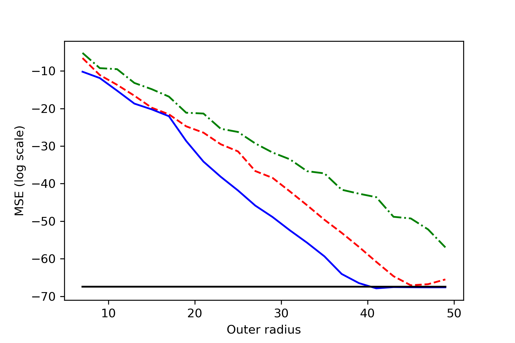
Figure 1: MSE for Lagrange and local Lagrange. The values for the outer radius are indicated on the horizontal axis as multiples of $\theta$. The values for the inner radius are $2\theta$, $3\theta$, $4\theta$. For the Lagrange basis, the three cases are visually similar, so they are represented by a single line. Solid black line: Lagrange basis; Dashed red line: Local Lagrange basis, $R_{i}=2\theta$; Solid blue line: Local Lagrange basis, $R_{i}=3\theta$; Dot-dash green line: Local Lagrange basis, $R_{i}=4\theta$.

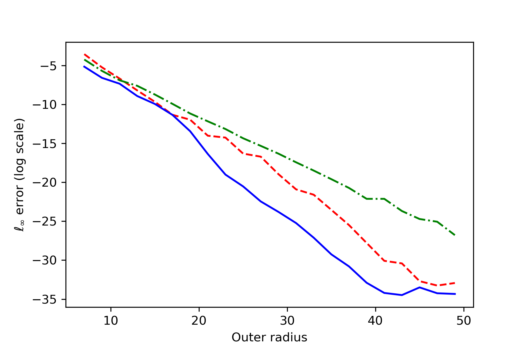
Figure 2: Error between a Lagrange and local Lagrange basis function in the $\ell_{\infty}$ norm. The values for the outer radius are indicated on the horizontal axis as multiples of $\theta$. The values for the inner radius are $2\theta$, $3\theta$, $4\theta$. Dashed red line: $R_{i}=2\theta$; Solid blue line: $R_{i}=3\theta$; Dot-dash green line: $R_{i}=4\theta$.

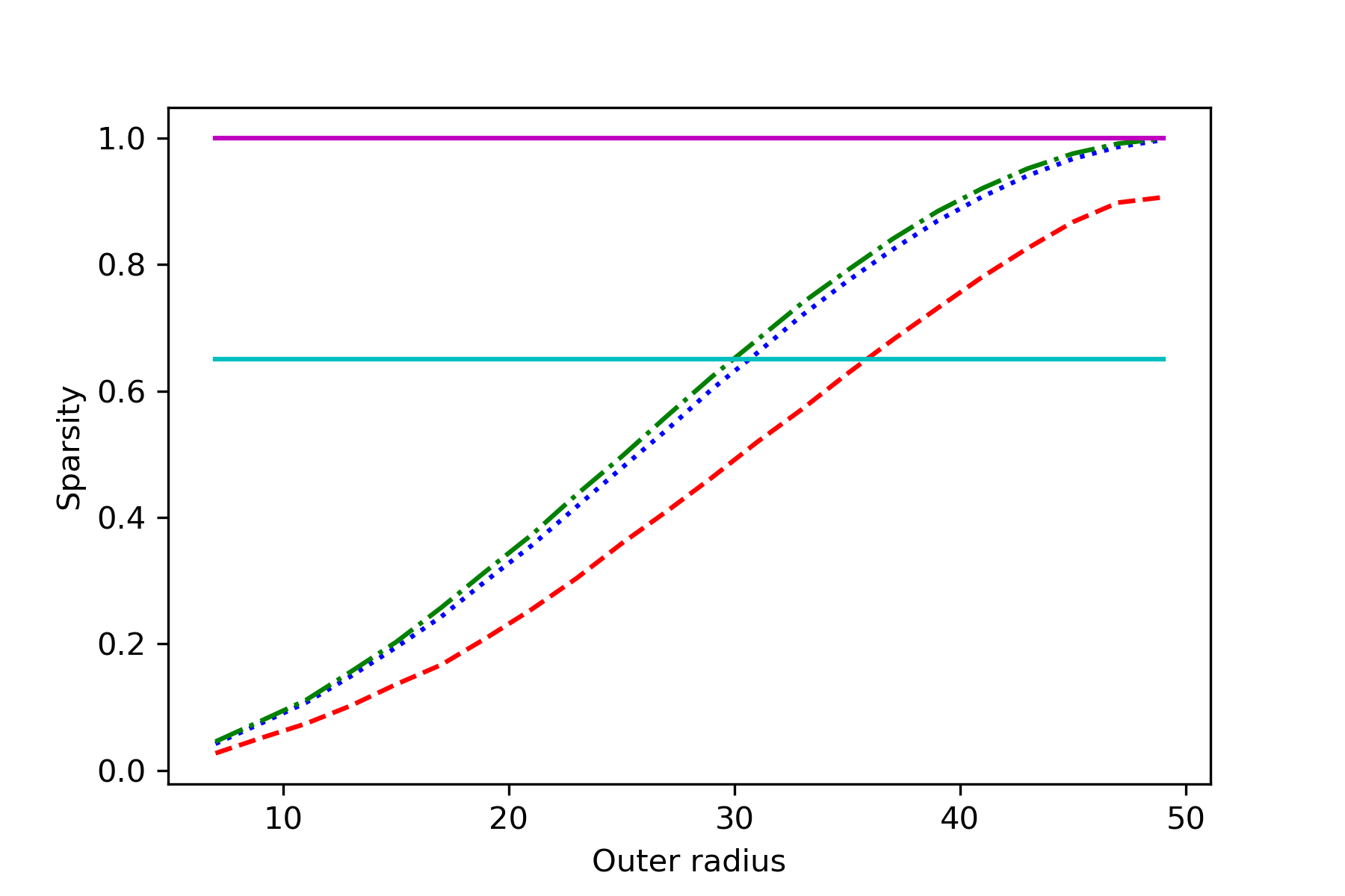
Figure 3: Sparsity of the bases as a ratio of nonzero entries in the basis matrix to the number of entries in the matrix. The values for the outer radius are indicated on the horizontal axis as multiples of $\theta$. The values for the inner radius are $2\theta$, $3\theta$, $4\theta$. Solid cyan line: Lagrange basis $R_{i}=2\theta$; Solid magenta line: Lagrange basis $R_{i}=3\theta$ and $R_{i}=4\theta$; Dashed red line: Local Lagrange basis $R_{i}=2\theta$; Dotted blue line: Local Lagrange basis $R_{i}=3\theta$; Dot-dash green line: Local Lagrange basis $R_{i}=4\theta$.

4.2 Computation time

We again consider points on the sphere that are located at the Fibonacci lattice points. For a range of numbers of points, we consider the time to compute the Lagrange and local Lagrange bases, cf. Figure 4. In each case, half of the data is considered known.

We also determine the time required to add a new vertex to the graph and recompute the local Lagrange bases, including updating the Laplacian as well as the neighborhoods of nearby points. Note that the global support of the Lagrange functions means that an update costs roughly the same as the original basis computation.

In this experiment, the local Lagrange basis functions are computed serially, and we see a linear trend to the computation time. The Lagrange functions are computed simultaneously as the solution of a minimization problem. However, as the number of vertices grows so do the matrices, making the computational time increase faster than that of the local Lagrange.

We expect that an efficient parallel implementation of the local Lagrange basis would show an even greater improvement in computation time over the Lagrange.

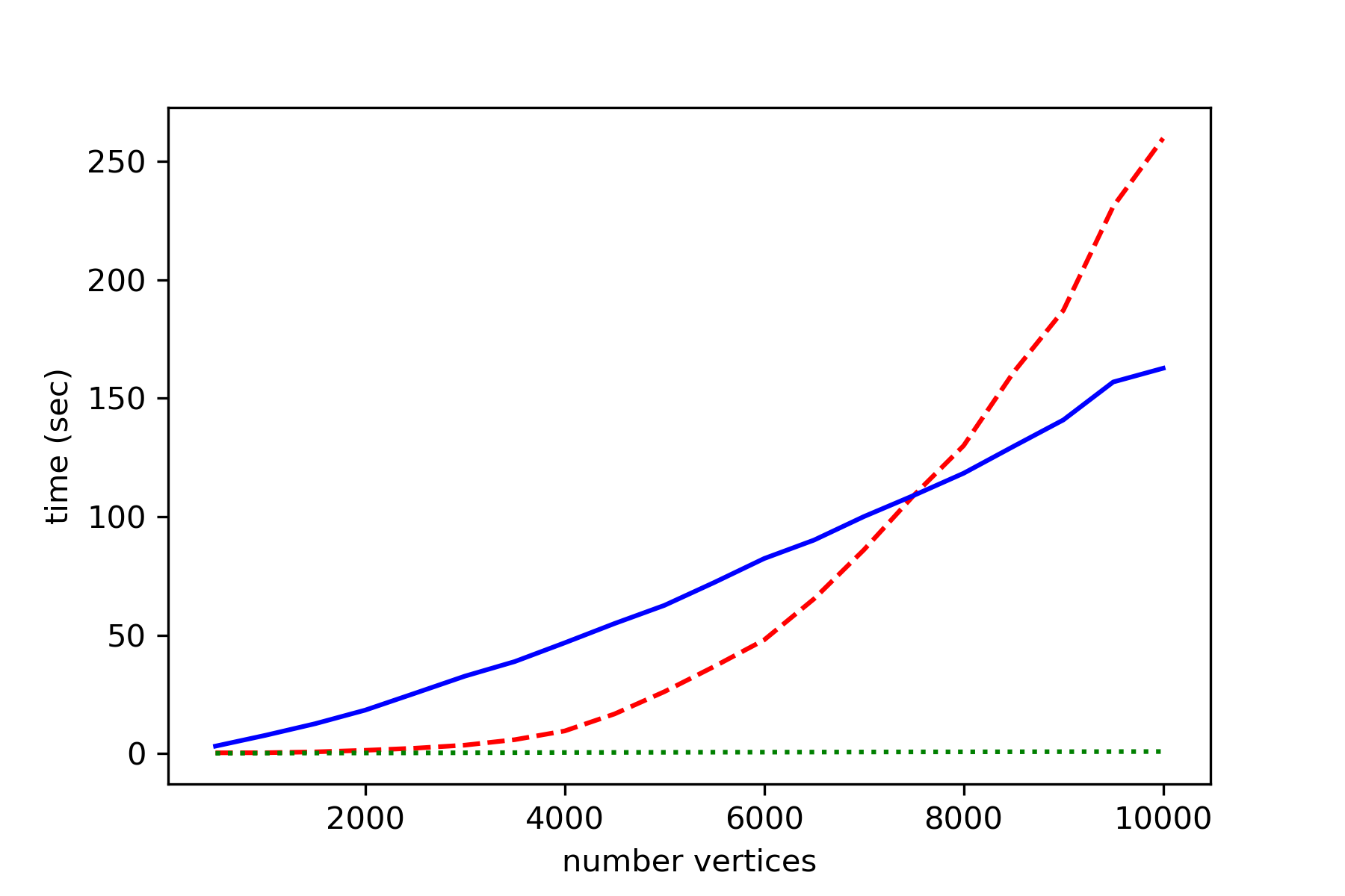
Figure 4: Computation time comparison between Lagrange and local Lagrange. Red dashed line: Lagrange basis; Solid blue line: Local Lagrange basis; Dotted green line: update of the local Lagrange basis after adding a vertex.

4.3 Energy performance of residential buildings

In a previous work [18], we considered a data set for energy efficiency of buildings. Two numerical values, Heating Load and Cooling Load, were predicted based on seven numeric parameters: Relative Compactness, Surface Area, Wall Area, Roof Area, Overall Height, Orientation, and Glazing Area. This data set is from the UC Irvine Machine Learning Repository [4], and it was used in [17]. There are 768 data points in this set.

As in the experiment of [18], we ran 20 simulations of 10-fold cross validation and measured the error of interpolation as mean squared error. This experiment is different from [18] in that we use a weighted $\ell_{1}$ norm to determine edge lengths, and we see that the refined graph construction provides a better approximation error. We rescale the distances so that every vertex has a neighbor within distance 1. We then compare the Lagrange and local Lagrange errors for a range of neighborhood radii. The results are reported in Table 1. We see that as the outer radius $R_{o}$ increases, the error of the local Lagrange interpolant converges to that of the Lagrange.

	Heating Load
$R_{o}$	Lagrange	Local Lagrange
3	0.2296 $\pm$ 0.0154	18.7001 $\pm$ 2.8098
4	0.2181 $\pm$ 0.0149	0.9574 $\pm$ 0.5161
5	0.2195 $\pm$ 0.0155	0.2284 $\pm$ 0.0212
6	0.2207 $\pm$ 0.0209	0.2207 $\pm$ 0.0209
7	0.2182 $\pm$ 0.0134	0.2182 $\pm$ 0.0134
8	0.2224 $\pm$ 0.0164	0.2224 $\pm$ 0.0164

Cooling Load
Lagrange	Local Lagrange
1.477 $\pm$ 0.1631	21.5409 $\pm$ 2.3183
1.4478 $\pm$ 0.1477	2.0827 $\pm$ 0.3261
1.5199 $\pm$ 0.2007	1.5334 $\pm$ 0.2059
1.7608 $\pm$ 1.0032	1.7608 $\pm$ 1.0032
1.6478 $\pm$ 0.7273	1.6478 $\pm$ 0.7273
1.4114 $\pm$ 0.1196	1.4114 $\pm$ 0.1196

Table 1: Energy performance (cf Table 1 of [18]). 10-fold cross-validation with 20 repetitions. Error metric: Mean Squared Error. The mean and standard deviation across the 20 simulations are reported. Note that the variation in the Lagrange error is solely due to the random shuffling of the data. In each row the same random shuffles were used for both methods.

Appendix A Positive definite matrices

It is possible that the following result is known. We were unable to find a reference, so we include a proof for the benefit of the reader.

Proposition A.1.

If $A$ is an $n\times n$ positive definite matrix, then

$$\inf_{\left\rVert y\right\rVert_{\infty}=1}\left\rVert Ay\right\rVert_{\infty}\geq\frac{2\lambda_{min}}{\sqrt{n}+1}$$ (5)

where $\lambda_{min}$ is the smallest eigenvalue of $A$. This implies

$$\left\rVert A^{-1}\right\rVert_{\infty}\leq\frac{\sqrt{n}+1}{2\lambda_{min}}.$$ (6)

Proof.

We consider $y$ vectors on the unit sphere with respect to the $\ell_{\infty}$ norm, and WLOG assume that they are in the non-negative cone, i.e. $y_{i}\geq 0$. First, note that $A=\lambda_{min}I+B$, where $B$ is positive semi-definite. For each $y$, let $By=\alpha_{1}y+\alpha_{2}\hat{y}$ where $\left\langle y,\hat{y}\right\rangle=0$. Since $B$ is positive semi-definite, $\alpha_{1}\geq 0$, and

$$\inf_{y}\left\rVert Ay\right\rVert_{\infty} =\inf_{y}\left\rVert\lambda_{min}y+\alpha_{1}y+\alpha_{2}\hat{y}\right\rVert_{\infty}$$

$$\geq\inf_{y}\inf_{w\in\mathbb{R}^{n},\left\langle y,w\right\rangle=0}\left\rVert(\lambda_{min}+\alpha_{1})y+w\right\rVert_{\infty}.$$

For each $y$, the optimal $w$ is in the affine hyperplane $\left\{y+w\ \middle|\ \left\langle y,w\right\rangle=0\right\}$. If all entries in $y$ are positive, the smallest $\ell_{\infty}$ ball about the origin that intersects this affine hyperplane will intersect it in the direction $e$, where $e$ denotes the vector with all values being 1. Otherwise, the intersection will be a space of larger dimension, but a point in the direction $e$ will still be in the intersection. Therefore, the minimum is attained for some point $(\lambda_{min}+\alpha_{1})y+w=\beta e$, with $y$ and $w$ making $\beta$ as small as possible. Then

$$\inf_{y}\left\rVert Ay\right\rVert_{\infty} \geq\left\rVert\beta e\right\rVert_{\infty}$$

$$=\beta.$$

Since $\left\langle y,w\right\rangle=0$, we also have

$$(\lambda_{min}+\alpha_{1})\left\rVert y\right\rVert_{2}^{2} =\left\langle y,(\lambda_{min}+\alpha_{1})y+w\right\rangle$$

$$=\left\langle y,\beta e\right\rangle$$

$$=\beta\left\rVert y\right\rVert_{1},$$

so

$$\inf_{y}\left\rVert Ay\right\rVert_{\infty} \geq\inf_{y}\frac{(\lambda_{min}+\alpha_{1})\left\rVert y\right\rVert_{2}^{2}}{\left\rVert y\right\rVert_{1}}$$

$$\geq\lambda_{min}\inf_{y}\frac{\left\rVert y\right\rVert_{2}^{2}}{\left\rVert y\right\rVert_{1}}$$

$$\geq\lambda_{min}\inf_{\bar{y}\in\mathbb{R}^{n-1}}\frac{1+\left\rVert\bar{y}\right\rVert_{2}^{2}}{1+\left\rVert\bar{y}\right\rVert_{1}}.$$

The greatest difference in the $\ell_{1}$ and $\ell_{2}$ norms occurs in the direction $\bar{e}\in\mathbb{R}^{n-1}$, all entries being 1. Hence

$$\inf_{y}\left\rVert Ay\right\rVert_{\infty} \geq\lambda_{min}\inf_{\bar{\beta}}\frac{1+\left\rVert\bar{\beta}\bar{e}\right\rVert_{2}^{2}}{1+\left\rVert\bar{\beta}\bar{e}\right\rVert_{1}}$$

$$=\lambda_{min}\inf_{\bar{\beta}}\frac{1+(n-1)\bar{\beta}^{2}}{1+(n-1)\bar{\beta}}.$$

Therefore, we want to minimize the function

$$f(a)=\frac{1+(n-1)a^{2}}{1+(n-1)a},$$

and the derivative is

$$f^{\prime}(a) =\frac{(n-1)((n-1)a^{2}+2a-1)}{(1+(n-1)a)^{2}}.$$

The minimum then occurs at

$$a=\frac{1}{\sqrt{n}+1},$$

and the corresponding value for $f$ is

$$\frac{2\sqrt{n}-2}{n-1}=\frac{2}{\sqrt{n}+1},$$

which establishes (5).

For (6), we have

$$\left\rVert A^{-1}\right\rVert_{\infty} =\sup_{z\neq 0}\frac{\left\rVert A^{-1}z\right\rVert_{\infty}}{\left\rVert z\right\rVert_{\infty}}.$$

Changing variables, we have

$$\left\rVert A^{-1}\right\rVert_{\infty} =\sup_{y\neq 0}\frac{\left\rVert y\right\rVert_{\infty}}{\left\rVert Ay\right\rVert_{\infty}}$$

$$=\frac{1}{\inf_{\left\rVert y\right\rVert=1}\left\rVert Ay\right\rVert_{\infty}}.$$

∎

References

- [1] J. J. Benedetto and P. J. Koprowski. Graph theoretic uncertainty principles. In Sampling Theory and Applications (SampTA), 2015 International Conference on, pages 357–361. IEEE, 2015.
- [2] F. R. K. Chung. Spectral graph theory, volume 92 of CBMS Regional Conference Series in Mathematics. Published for the Conference Board of the Mathematical Sciences, Washington, DC; by the American Mathematical Society, Providence, RI, 1997.
- [3] D. I Shuman, M. J. Faraji, and P. Vandergheynst. A multiscale pyramid transform for graph signals. IEEE Trans. Signal Process., 64(8):2119–2134, Apr. 2016.
- [4] D. Dheeru and E. Karra Taniskidou. UCI machine learning repository, 2017.
- [5] W. Erb. Graph signal interpolation with positive definite graph basis functions. arXiv preprint arXiv:1912.02069, 2019.
- [6] W. Erb. Semi-supervised learning on graphs with feature-augmented graph basis functions. arXiv preprint arXiv:2003.07646, 2020.
- [7] E. Fuselier, T. Hangelbroek, F. J. Narcowich, J. D. Ward, and G. B. Wright. Localized bases for kernel spaces on the unit sphere. SIAM J. Numer. Anal., 51(5):2538–2562, 2013.
- [8] T. Hangelbroek, F. Narcowich, C. Rieger, and J Ward. An inverse theorem for compact Lipschitz regions in using localized kernel bases. Mathematics of Computation, 87(312):1949–1989, 2018.
- [9] J. Jiang, C. Cheng, and Q. Sun. Nonsubsampled graph filter banks: Theory and distributed algorithms. IEEE Transactions on Signal Processing, 67(15):3938–3953, 2019.
- [10] M. S. Kotzagiannidis and P. L. Dragotti. Splines and wavelets on circulant graphs. Applied and Computational Harmonic Analysis, 47(2):481 – 515, 2019.
- [11] I. Pesenson. Sampling in Paley-Wiener spaces on combinatorial graphs. Trans. Amer. Math. Soc., 360(10):5603–5627, 2008.
- [12] I. Pesenson. Variational splines and paley–wiener spaces on combinatorial graphs. Constructive Approximation, 29(1):1–21, Feb 2009.
- [13] I. Pesenson. Removable sets and approximation of eigenvalues and eigenfunctions on combinatorial graphs. Applied and Computational Harmonic Analysis, 29(2):123 – 133, 2010.
- [14] D. I Shuman. Localized spectral graph filter frames: A unifying framework, survey of design considerations, and numerical comparison. arXiv preprint arXiv:2006.11220, 2020.
- [15] D.I. Shuman, S.K. Narang, P. Frossard, A. Ortega, and P. Vandergheynst. The emerging field of signal processing on graphs: Extending high-dimensional data analysis to networks and other irregular domains. IEEE Signal Processing Magazine, 30(3):83–98, 2013.
- [16] A.J. Smola and R. Kondor. Kernels and regularization on graphs. In Learning theory and kernel machines, pages 144–158. Springer, 2003.
- [17] A. Tsanas and A. Xifara. Accurate quantitative estimation of energy performance of residential buildings using statistical machine learning tools. Energy and Buildings, 49:560 – 567, 2012.
- [18] J. P. Ward, F. J. Narcowich, and J. D. Ward. Interpolating splines on graphs for data science applications. Applied and Computational Harmonic Analysis, 49(2):540 – 557, 2020.
- [19] D. S. Watkins. Fundamentals of matrix computations, volume 64. John Wiley & Sons, 2004.