Net-baryon number fluctuationsNet-baryon number fluctuations C. Schmidt et al.

Abstract

The appearance of large, none-Gaussian cumulants of the baryon number distribution is commonly discussed as a signal for the QCD critical point. We review the status of the Taylor expansion of cumulant ratios of baryon number fluctuations along the freeze-out line and also compare QCD results with the corresponding proton number fluctuations as measured by the STAR Collaboration at RHIC. To further constrain the location of a possible QCD critical point we discuss poles of the baryon number fluctuations in the complex plane. Here we use not only the Taylor coefficients obtained at zero chemical potential but perform also calculations of Taylor expansion coefficients of the pressure at purely imaginary chemical potentials.

12.38.Mh, 25.75.Nq

1 Introduction

The phase diagram of Quantum Chromodynamics (QCD) is currently investigated with large efforts by means of heavy ion experiments at LHC and RHIC, as well as by numerical calculations of lattice regularized QCD. While lattice calculations at vanishing chemical potential made great progress in the last decades, they are still harmed by the infamous sign problem at nonzero chemical potential. The two main methods that are currently used to infer on the QCD phase diagram at nonzero baryon chemical potential $(\mu_{B})$ are indirect, they rely on Taylor expansions of observables at $\mu_{B}=0$, or analytical continuations from simulations at imaginary chemical potential ($\mu_{B}=i\mu_{I}$). Methods that allow for a direct sampling of the oscillatory path integral at $(\mu_{B})>0$ are currently investigated, see e.g. [1, 2].

The two principles that are guiding our understanding of the QCD phase diagram are spontaneous chiral symmetry breaking and – linked to it – the phenomena of quark confinement. Our knowledge on the (2+1)-flavor QCD phase diagram based on recent lattice results is summarized in Fig. 1 (left).

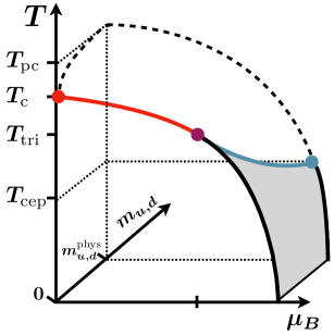
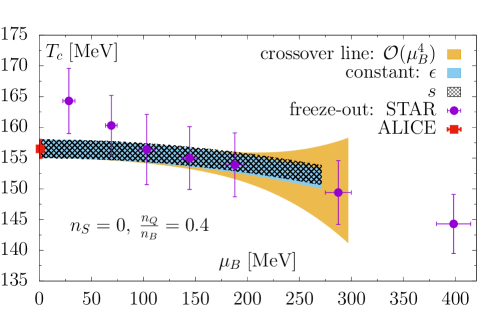
Figure 1: Left: Schematic picture of the QCD phase diagram. The chiral limit ($m_{u,d}=0$) is shown in the front, whereas the physical mass case is shown in the back. Right: The chiral crossover line in 2 + 1 flavor QCD, calculated with the constraints $n_{S}=0$ and $n_{Q}=0.4n_{B}$. It is compared with the line of constant energy density $\epsilon=0.42(6)GeV/fm^{3}$ and the line of constant entropy density $s=3.7(5)fm^{-3}$ [3] in the $T-\mu_{B}$ plane. Also, shown are the chemical freeze-out parameters extracted from grand canonical ensemble based fits to hadron yields for the ALICE [4] and the STAR [5] experiments.

The variables assigned to the three axes are temperature ($T$), the baryon chemical potential ($\mu_{B}$) and light quark mass ($m_{u,d}$). At low $T$ and low $\mu_{B}$ the chiral symmetry is spontaneously broken and quarks are confined into hadrons. Correspondingly, chiral symmetry is restored at high $T$ and high $\mu_{B}$, where quarks can move freely. Solid red and cyan lines indicate a continous phase transition in the universality class of the 3d-O(4) symmetric spin model, or the Z(2) symmetric Ising model, respectively. Black lines and gray surfaces indicate a discontinuous first order transition. On the temperature axis we also indicate the pseudo critical transition temperature at physical masses ($T_{pc}$), the critical temperature in the chiral limit ($T_{c}$), the temperature of the tri-critical point in the chiral limit ($T_{tri}$) and the temperature of the critical (end-)point at physical quark masses ($T_{cep}$). It emerges a hierarchy as $T_{pc}>T_{c}>T_{tri}>T_{cep}$. The first two temperatures are determined by lattice calculations as $T_{pc}=156(\pm 1.5)$ MeV [6] and $T_{c}=132^{+3}_{-6}$ MeV [7]. The variation of $T_{pc}$ with $\mu_{B}$, as indicated by a dashed line, has also been calculated by lattice QCD. We obtain

$$\frac{T_{pc}(\mu_{B})}{T_{pc}(0)}=1-\kappa_{2}\left(\frac{\mu_{B}}{T}\right)^{2}+\mathcal{O}\left(\frac{\mu_{B}}{T}\right)^{4},$$ (1)

where $\kappa_{2}^{B}=0.012(4)$ with a $\mathcal{O}(\mu_{B}^{4})$ correction that vanishes within errors [6]. Similar results have been obtained recently in Ref. [8].

In Fig. 1 (right) we compare the pseudo-critical line with freeze-out temperatures and chemical potentials obtained from hadron yields measured by STAR [5] and ALICE [4]. The hadron yields have been fitted (after feed-down corrections) to the hadron resonance gas (HRG) model. In its simplest none-interacting version, this model is based on the mass spectrum of all stable particles and resonances listed in the particle data booklet, which are taken as an ideal gas in thermal equilibrium at a common temperature $T_{f}$, chemical potential $\mu_{f}$, and volume $V_{f}$. As these parameters refer to the time in the expansion of the fireball from when on its chemical composition does not change anymore, they are called chemical freeze-out parameters. We see from Fig. 1 (right), that the freeze-out parameters agree well with the chiral crossover line obtained from lattice QCD. We note, that in order to meet conditions that are found in heavy ion collisions we have determined our values for the electric $\mu_{Q}\equiv\mu_{Q}(\mu_{B})$ and strangeness chemical potentials $\mu_{S}\equiv\mu_{S}(\mu_{B})$, such that the following conditions for the net-numbers of conserved charges in the system, $\left<n_{Q}/n_{B}\right>=0.4$ and $\left<n_{S}\right>=0$, are fulfilled. However, the freeze-out parameters are still model based. Hence, in the following we want to follow a procedure proposed in [9], that allow for the determination of the freeze-out parameters by a direct comparison of lattice QCD to experiment.

2 Cumulants of net-baryon number

Higher order cumulants of the net-baryon number are obtained as derivatives of the logarithm of the QCD partition functions with respect to the dimension less parameter $\hat{\mu}_{B}=\mu_{B}/T$,

$$\chi_{n}^{B}(T,\mu_{B},\mu_{Q},\mu_{S})=\frac{1}{VT^{3}}\frac{\partial^{n}\ln Z(T,\mu_{B},\mu_{Q},\mu_{S})}{\partial\hat{\mu}_{B}^{n}},$$ (2)

where $\mu_{Q}$ an $\mu_{S}$ are the electric charge and strangeness chemical potentials. In the same way, we can can also calculate derivatives with respect to $\mu_{Q}$ and $\mu_{S}$, which we denote as $\chi_{n}^{Q}$ and $\chi_{n}^{S}$, respectively.

Aiming on the comparison with the experimental results, we further introduce ratios of cumulants of baryon number fluctuations as

$$R_{nm}^{B}=\frac{\chi_{n}^{B}}{\chi_{m}^{B}}.$$ (3)

By using these ratios, the leading order dependence on the freeze-out volume ($V^{f}$) is removed. However, among other things fluctuations of the experimentally observed freeze-out volume might still hinder a comparison to lattice QCD. The first ratio we discuss is $R_{12}^{B}$, which is shown in Fig. 2

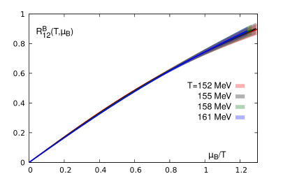
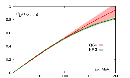
Figure 2: Left: Continuum estimate of the cumulant ratio $R_{12}^{B}$ as function of the chemical potential, for different temperatures. Right: The same ratio along the pseudo critical line. Shown are the QCD and HRG model results.

and can be interpreted as the mean of the net-baryon number, normalized by the variance of the baryon number fluctuations. The presented HotQCD results [10] are obtained from high statistics lattice QCD calculations on $32^{3}\times 8$ and $48^{3}\times 12$ lattices, with (2+1)-flavor of highly improved staggered quarks (HISQ) at physical light and strange quark masses. The values in the range $0<\hat{\mu}_{B}\lesssim 1.2$ stem from a Taylor expansion of the logarithm of the partition function about $\hat{\mu}_{B}=0$ to $8^{th}$ order in $\hat{\mu}_{B}$. As it is evident from the continuum estimate shown in Fig. 2 (left), the leading order of $R_{12}^{B}$ is linear in $\mu_{B}$. We further notice that the ratio is rather independent under the variation of temperature. Therefore the ratio has been termed a baryometer [9].

The same ratio is shown in Fig. 2 (right), now plotted along the pseudo critical line as defined in Eq. (1). Here we compare the QCD result with the corresponding calculation of a Hadron Resonance Gas (HRG). We see that the HRG model deviates from QCD only for $\mu_{B}\gtrsim 150$ MeV. We thus note that for small $\mu_{B}$ the HRG can be used to analyse the differences between net-baryon number and net-proton number fluctuations. The latter is the quantity which is directly accessible by heavy ion experiments. On the other hand, this also means that we do not see any indication of a diverging baryon number fluctuation ($\chi_{2}^{B}$) in the range where we trust our Taylor expansion, which we would expect in QCD close to a critical point. In this case the ratio $R_{12}^{B}$ would decrease and approach zero at the critical point.

As higher order cumulants are expected to diverge more rapidly when approaching a critical point, it is tempting to discuss also the ratios $R_{31}^{B}$ and $R_{42}^{B}$ along the pseudo critical line, which are shown in Fig. 3 as a function of $R_{12}^{B}$ [10]. Since $R_{12}^{B}$ is still a monotonous function of $\mu_{B}$ in the plotted range, it is a measure for the baryon density and enables us to compare with the experiment in a model free way.

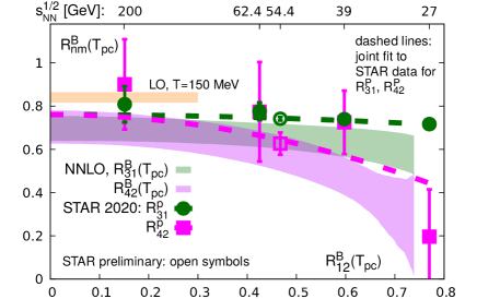
Figure 3: The cumulant ratios (bands) $R_{31}^{B}$ and $R_{42}^{B}$ versus $R_{12}^{B}$ on the pseudo-critical line, calculated from a NNLO Taylor series. Data are results on cumulant ratios of net-proton number fluctuations obtained by the STAR Collaboration [11]. Also shown are preliminary results obtained at $\sqrt{s_{NN}}=54.4$ GeV [12]. Dashed lines show joint fits to the data.

We see that the over all agreement with the corresponding net-proton number cumulants $R_{31}^{P}$ and $R_{42}^{P}$ from STAR [11, 12] is very good. We conclude that a high freeze-out temperature of $T^{f}>155$ MeV seems to be excluded by the data. This lattice calculation is based on an $8^{th}$ order expansion of the logarithm of the partition function.

Finally we want to mention that the radius of convergence, which is inherent to the expansion of any thermodynamic observable, can in principle provide valuable information on the phase structure of QCD. E.g., in the case of a second order phase transition, we expect the convergence radius to be limited by the critical point. A simple estimator for the radius of convergence $\hat{\rho}\equiv\mu_{B}^{\textrm{crit}}/T$ is given by the ratio estimator

$$\hat{\rho}=\lim_{n\to\infty}\sqrt{(n+2)(n+1)\left|\chi_{n}^{B}/\chi_{n+2}^{B}\right|},$$ (4)

more advanced estimators are also discussed [13]. Unfortunately, we have only a limited number of expansion coefficients (cumulatns $\chi_{n}^{B}$) at our disposal, which makes it difficult to draw strong conclusions with given lattice data. Especially, since the statistical and systematical error on higher order cumulants is drastically increasing with the order $n$. It is however interesting to note that all expansion coefficients have to be positive if the limiting singularity lies on the real axis. Hence, we can obtain an upper bound for the phase transition temperature $T_{cep}$, as for $T>140$ MeV many of the expansion coefficients turn negative [14]. This estimate is in good agreement with the statement that the temperature of the QCD critical point shall be lower than the chiral transition temperature ($T_{cep}<T_{c}$) as indicated in Fig. 1 (left).

3 Cumulants at imaginary chemical potential

Besides the Taylor expansion method, lattice QCD calculations can also be performed at purely imaginary chemical potential, followed by an analytic continuation of the results. The QCD partition function is symmetric under the transformation $\hat{\mu}_{B}\to\hat{\mu}_{B}+2\pi i$. Any simulations at imaginary chemical potential are thus constrained to the interval $[-i\pi,i\pi]$ (first Roberge-Weiss sector). We further note that even/odd order cumulants on this interval are purely real/imaginary and are even/odd functions of $\textrm{Im}[\hat{\mu}_{B}]$. Making use of this symmetry, we thus need to simulate only in the interval $[0,i\pi]$ and symmetrize/anti-symmetrize the data afterwards. We calculate the first four cumulants of the baryon number. Preliminary results from $24^{3}\times 4$ lattices are shown in Fig. 4.

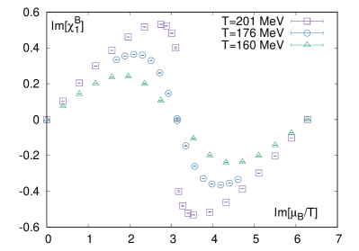
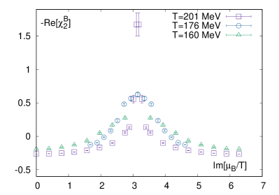
Figure 4: Preliminary results of the first and second cumulant of the net-baryon number, $\chi_{1}^{B}$, $\chi_{2}^{B}$, as a function of the imaginary chemical potential for three different temperatures, obtained from calculations on $24^{3}\times 4$ lattices.

We can see that the (purely imaginary) baryon number density $\textrm{Im}[\chi_{1}^{B}]$ develops a discontinuity at $\textrm{Im}[\hat{\mu}_{B}]=\pi$. The temperature where this is happening is called the Roberge-Weiss temperature ($T_{RW}$), which was estimated to $T_{RW}=201$ MeV [15] (for $N_{\tau}=4)$. In accordance with this discontinuity, we also observe that the second cumulant $\chi_{2}^{B}$ develops a divergence at $T_{RW}$. The universal scaling of the Polyakov-Loop (order parameter of the confinement transition) and chiral condensate have been investigated close to the Roberge-Weiss transition [15].

The periodic data on $\chi_{1}^{B}$ can be analyzed in terms of Fourier coefficients [16, 17], which are inherently linked to the canonical partition sums. The aim of this project is, however, to use the information of all the available cumulants to construct a precise rational function approximation, i.e. a $[n,m]$ Padé of $\chi_{1}^{B}$,

$$\chi_{1}^{B}\approx\mathcal{R}^{m}_{n}(\hat{\mu}_{B})=\frac{P_{m}}{Q_{n}}=\frac{\sum_{i=0}^{m}\,a_{i}\,\hat{\mu}_{B}^{i}}{\sum_{j=0}^{n}\,b_{j}\,\hat{\mu}_{B}^{j}}.$$ (5)

We are currently testing several methods to determine the coefficients $a_{i},b_{j}$. Among them is a direct solve method, where we directly solve a set of equations that we obtain by equating the analytic expressions for $\mathcal{R}^{m}_{n}$ as well as its first few derivatives $\partial^{j}\mathcal{R}^{m}_{n}/\partial\hat{\mu}_{B}^{j}$, $j=0,1,2$ at each simulation point with our lattice data,

$$\chi_{j+1}^{B}(\hat{\mu}_{B}^{(k)})=\left.\frac{\partial^{j}\mathcal{R}^{m}_{n}(\hat{\mu}_{B})}{\partial\hat{\mu}_{B}^{j}}\right|_{\hat{\mu}_{B}=\hat{\mu}_{B}^{(k)}}.$$ (6)

Here $\chi_{j}^{B}(\hat{\mu}_{B}^{(k)})$ represent the numerical values of the cumulants at the simulation points $\hat{\mu}_{B}^{(k)}$, as obtained by our lattice calculations. A similar method is based on a $\chi^{2}$-fit of $\mathcal{R}^{m}_{n}$ to our cumulant data. Finally we are testing a two step approach where in a first step a suitable interpolation of the lattice data is chosen. In the second step we are making use of the Remez algorithm to determine $\mathcal{R}^{m}_{n}$ until the min-max criteria is satisfied with respect to the interpolation.

Having the approximation $\mathcal{R}^{m}_{n}$ at hand, we are able to integrate the baryon density to obtain the free energy, which will also develop a cusp at $T_{RW}$. However, our main interest lies in the determination of the roots of the numerator $P_{m}$ and denominator $Q_{n}$, which will allow us to infer information on the singularities in the complex $\hat{\mu}_{B}$ plane. A singularity in the complex plane is the reason for a finite radius of convergence of the Taylor series and will also indicate a true physical phase transition when it approaches the real axis in the complex $\hat{\mu}_{B}$-plane.

There are two models that can guide our thinking about the location of the singularities in the complex plane. At large temperatures the thermal branch cut singularities from the Fermi-Dirac distribution of a free quark gas is expected to pinch the imaginary axis in the complex $\hat{\mu}_{B}$-plane. In QCD such a behavior is expected to happen at $T_{RW}$. In fact, this is something we already see, when we analyze the data shown in Fig. 4. How this thermal singularity moves in the complex plane with with decreasing temperature is shown in Fig. 5 (left).

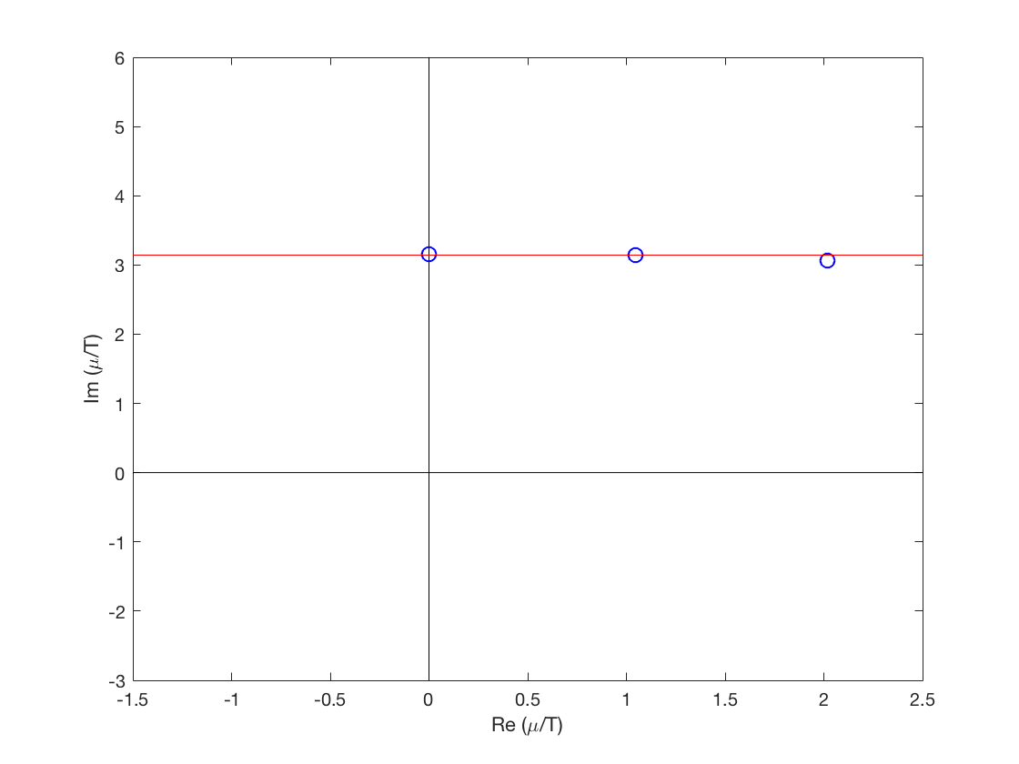
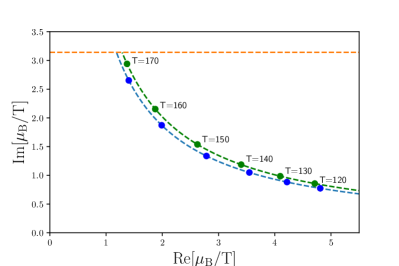
Figure 5: Left: Singularity in the complex plane, associated with the branch cut singularity of the Fermi-Dirac distribution function of the quarks. The position of the singularity is shown for three temperatures $T=201,176$ and $160$ MeV from left to right. The results have been obtained from calculations on $24^{3}\times 4$ lattices. Right: Singularity in the complex plane, associated to the pole in the scaling function $f_{f}(z)$. The results are model predictions for $N_{\tau}=4,6$ (blue, green) based on a mapping of QCD to the universal 3d $O(2)$-model.

At temperatures close to the chiral transition ($T_{c}$), we might be able to map our results to the universal scaling behavior connected to the chiral phase transition. The scaling function of the free energy $f_{f}(z)$ will have a singularity in the complex $z$-plane, known as the Lee-Yang edge singularity. This singularity has been determined recently [18]. Given a mapping from QCD to the universal theory, defined by the non-universal constants $t_{0},h_{0},T_{c},\kappa_{2}^{B}$ [HotQCD, private communication], we can calculate the position of the singularity in the complex $\hat{\mu}_{B}$-plane, shown in Fig. 5 (right). Preliminary results from calculations on $36^{3}\times 6$ lattices at $T=145$ MeV seem to be in rather good agreement with this prediction. It will be very interesting but also challenging to see if the singularity will approach the real axis in the complex $\hat{\mu}_{B}$-plane for even smaller temperatures.

References

- [1] Felipe Attanasio, Benjamin Jäger and Felix P.G. Ziegler “Complex Langevin simulations and the QCD phase diagram: Recent developments” In Eur. Phys. J. A 56.10, 2020, pp. 251 DOI: 10.1140/epja/s10050-020-00256-z
- [2] Andrei Alexandru, Gokce Basar, Paulo F. Bedaque and Neill C. Warrington “Complex Paths Around The Sign Problem”, 2020 arXiv:2007.05436 [hep-lat]
- [3] A. Bazavov “The QCD Equation of State to from Lattice QCD” In Phys. Rev. D 95.5, 2017, pp. 054504 DOI: 10.1103/PhysRevD.95.054504
- [4] Anton Andronic, Peter Braun-Munzinger, Krzysztof Redlich and Johanna Stachel “Decoding the phase structure of QCD via particle production at high energy” In Nature 561.7723, 2018, pp. 321–330 DOI: 10.1038/s41586-018-0491-6
- [5] L. Adamczyk “Bulk Properties of the Medium Produced in Relativistic Heavy-Ion Collisions from the Beam Energy Scan Program” In Phys. Rev. C 96.4, 2017, pp. 044904 DOI: 10.1103/PhysRevC.96.044904
- [6] A. Bazavov “Chiral crossover in QCD at zero and non-zero chemical potentials” In Phys. Lett. B 795, 2019, pp. 15–21 DOI: 10.1016/j.physletb.2019.05.013
- [7] H.T. Ding “Chiral Phase Transition Temperature in ( 2+1 )-Flavor QCD” In Phys. Rev. Lett. 123.6, 2019, pp. 062002 DOI: 10.1103/PhysRevLett.123.062002
- [8] Szabolcs Borsanyi et al. “QCD Crossover at Finite Chemical Potential from Lattice Simulations” In Phys. Rev. Lett. 125.5, 2020, pp. 052001 DOI: 10.1103/PhysRevLett.125.052001
- [9] A. Bazavov “Freeze-out Conditions in Heavy Ion Collisions from QCD Thermodynamics” In Phys. Rev. Lett. 109, 2012, pp. 192302 DOI: 10.1103/PhysRevLett.109.192302
- [10] A. Bazavov “Skewness, kurtosis, and the fifth and sixth order cumulants of net baryon-number distributions from lattice QCD confront high-statistics STAR data” In Phys. Rev. D 101.7, 2020, pp. 074502 DOI: 10.1103/PhysRevD.101.074502
- [11] J. Adam “Net-proton number fluctuations and the Quantum Chromodynamics critical point”, 2020 arXiv:2001.02852 [nucl-ex]
- [12] Ashish Pandav “Measurement of cumulants of conserved charge multiplicity distributions in Au +Au collisions from the STAR experiment” In Nucl. Phys. A 1005, 2021, pp. 121936 DOI: 10.1016/j.nuclphysa.2020.121936
- [13] Matteo Giordano and Attila Pásztor “Reliable estimation of the radius of convergence in finite density QCD” In Phys. Rev. D 99.11, 2019, pp. 114510 DOI: 10.1103/PhysRevD.99.114510
- [14] Frithjof Karsch “Critical behavior and net-charge fluctuations from lattice QCD” In PoS CORFU2018, 2019, pp. 163 DOI: 10.22323/1.347.0163
- [15] Jishnu Goswami, Frithjof Karsch, Anirban Lahiri and Christian Schmidt “QCD phase diagram for finite imaginary chemical potential with HISQ fermions” In PoS LATTICE2018, 2018, pp. 162 DOI: 10.22323/1.334.0162
- [16] Volodymyr Vovchenko, Jan Steinheimer, Owe Philipsen and Horst Stoecker “Cluster Expansion Model for QCD Baryon Number Fluctuations: No Phase Transition at ” In Phys. Rev. D 97.11, 2018, pp. 114030 DOI: 10.1103/PhysRevD.97.114030
- [17] Gabor Andras Almasi et al. “Fourier coefficients of the net-baryon number density and chiral criticality” In Phys. Rev. D 100.1, 2019, pp. 016016 DOI: 10.1103/PhysRevD.100.016016
- [18] Andrew Connelly, Gregory Johnson, Fabian Rennecke and Vladimir Skokov “Universal Location of the Yang-Lee Edge Singularity in Theories” In Phys. Rev. Lett. 125.19, 2020, pp. 191602 DOI: 10.1103/PhysRevLett.125.191602