PROCEEDINGS OF THE SECOND MADANALYSIS 5 WORKSHOP ON LHC RECASTING IN KOREA

Abstract

We document the activities performed during the second MadAnalysis 5 workshop on LHC recasting, that was organised in KIAS (Seoul, Korea) on February 12-20, 2020. We detail the implementation of 12 new ATLAS and CMS searches in the MadAnalysis 5 Public Analysis Database, and the associated validation procedures. Those searches probe the production of extra gauge and scalar/pseudoscalar bosons, supersymmetry, seesaw models and deviations from the Standard Model in four-top production.

1 Introduction

By Jack Y. Araz, Eric Conte, Robin Ducrocq, Thomas Flacke, Benjamin Fuks, Si Hyun Jeon, Taejeong Kim, Pyungwon Ko, Seung J. Lee, Richard Ruiz and Dipan Sengupta

Whereas the discovery of the Higgs boson almost a decade ago has accomplished one of the main objectives of the LHC physics program, no significant deviation beyond the Standard Model of particle physics has been found so far by the LHC experiments. Therefore, the concrete mechanism triggering the breaking of the electroweak symmetry remains unexplained, and no hint for any solution to the issues and limitations (such as the hierarchy problem, neutrino masses, dark matter, etc.) of the Standard Model has emerged from data. As new physics must exist in some form, data therefore implies that either the new states are too heavy and/or their interactions too feeble to leave any observable signature within the present collider reach, or that new particles lie in a configuration rendering their discovery challenging.

As a consequence of this non-observation of any new phenomenon at colliders, the results of the experimental searches are traditionally interpreted as constraints on various theoretical models. These include popular scenarios like the Minimal Supersymmetric Standard Model, as well as simplified models or effective field theories. There is, however, a vast domain of new physics setups extending the Standard Model, which all come with a variety of concrete realisations and whose predictions should be compared with LHC data. It is therefore crucial to develop a strategy allowing to exploit in the best possible way the current and future results of the LHC, so that one could straightforwardly draw conclusive statements on what physics beyond the Standard Model could or could not be.

Many groups have consequently developed and maintained public programs dedicated to the re-interpretation of the results of the LHC [1, 2, 3, 4, 5]. In practice, these programs aim to predict the number of signal events that populate the different signal regions of given LHC analyses, when one assumes a specific new physics context. From those predictions, considered together with information on data and on the Standard Model expectation, it becomes possible to derive whether the considered new physics scenario is excluded. MadAnalysis 5 and its public analysis database (PAD) is one of these tools [6, 7, 3, 8].

The strategy that MadAnalysis 5 follows relies on the generation of Monte Carlo signal events representative of the signature(s) of a given model of physics beyond the Standard Model. Those events are generated by relying on calculations matching fixed order results with parton showers, and they are further processed to include the modelling of hadronisation and multiple parton interactions. Hadron-level events are handled to simulate the response of the ATLAS or CMS detector, which can be either achieved with the Delphes 3 software [9] or with the simplified SFS fast detector simulation shipped with MadAnalysis 5[10]. Next, the detector-level events are reconstructed and the code derives, by employing validated and dedicated C++ recast codes, how those events populate the signal regions of the different analyses of the PAD. From those predictions, as above-mentioned, a statistical treatment allows for the derivation of conclusions about whether the initially considered model of new physics is excluded, and at which confidence level.

While implementing existing ATLAS and CMS searches in the MadAnalysis 5 framework is not complicated per se, as this consists in transcribing in C++ and in the code’s internal data format a given search as described in the experimental publications, doing so in a robust and trustable way is more difficult[11, 3, 12]. This indeed requires a careful validation of the implementation, which can be achieved in several manners. For instance, one could derive cut-flows for well-defined new physics scenarios, and compare them, on a cut-by-cut basis, with the corresponding official results. One could also compare the shapes of various differential distributions at different steps of the cut-flow with the corresponding ATLAS or CMS curves, and finally, it is also possible to extract exclusion contours for dedicated new physics frameworks, and confront them to their official counterpart. In those comparison, we expect to obtain an agreement at a satisfactory level, the precise definition of this level being dependent on the analysis through (variable) quality of the associated validation material released by the ATLAS and CMS collaborations.

In these proceedings, we report the activities that have been performed during the second MadAnalysis 5 workshop in Korea, that was held at the Korea Institute for Advanced Study (KIAS) in Seoul (South Korea), on February 12-20, 2020. Similar to its 2017 edition [13], the workshop brought together an enthusiastic group of students with post-doctoral, junior and senior researchers. Along with the main theme of the workshop, namely the re-interpretation of the results of the LHC searches for new physics, various lectures on collider physics, beyond the standard model theories and LHC experimental aspects were organised, together with dedicated sessions on Monte Carlo event generation and MadAnalysis 5.

The scope of the workshop consisted of a recasting exercise assigned to the participants, who were tasked with implementing in the MadAnalysis 5 framework several particular ATLAS and CMS searches for new physics. Moreover, a careful validation of these implementations was required, so that they could be shared with the community for dedicated physics studies without any concern. These proceedings document those implementations and their validation. Twelve new analyses have been added to the PAD as an outcome of the workshop. Their source codes are available from the MadAnalysis 5 dataverse, often with the Monte Carlo configuration cards relevant for the validation of the different implementations. More details and validation information can be found in the following sections.

The list of analyses under consideration is provided below:

1. ATLAS-EXOT-2018-30: an ATLAS search for $W^{\prime}$-boson production and decay into a lepton-neutrino pair with 139 fb^-1 of LHC data [14]; see https://doi.org/10.14428/DVN/GLWLTF [15] and section 2.

2. CMS-EXO-17-015: a CMS search for leptoquark pair-production, followed by decays into dark matter, one muon and one jet with 77.4 fb^-1 of LHC collisions [16]; see https://doi.org/10.14428/DVN/ICOXG9[17] and section 3.

3. CMS-EXO-17-030: a CMS search for the pair production of a new physics state decaying into three jets with 35.9 fb^-1 of LHC collisions [18]; see https://doi.org/10.14428/DVN/GAZACQ [19] and section 4;

4. CMS-EXO-19-002: a CMS search for new physics in final states containing multiple leptons with 137 fb^-1 of LHC collisions [20]; see https://doi.org/10.14428/DVN/DTYUUE [21] and section 5;

5. CMS-HIG-18-011: a CMS search for exotic Higgs decays into a di-muon and di-$b$-jet system via two pseudo-scalars with 35.9 fb^-1 of LHC collisions [22]; see https://doi.org/10.14428/DVN/UOH6BF [23] and section 6;

6. ATLAS-SUSY-2018-04: an ATLAS search for the pair production of staus that each decay into a tau lepton and missing transverse energy, with 139 fb^-1 of LHC collisions [24]; see https://doi.org/10.14428/DVN/UN3NND [25] and section 7;

7. ATLAS-SUSY-2018-06: an ATLAS search for electroweakino pair production and decay through Jigsaw variables, with 139 fb^-1 of LHC collisions [26]; see https://doi.org/10.14428/DVN/LYQMUJ [27] and section LABEL:sec:jigsaw;

8. ATLAS-SUSY-2018-31: an ATLAS search for sbottom pair production and decay in the multi-bottom plus missing transverse energy channel, with 139 fb^-1 of LHC collisions [28]; see https://doi.org/10.14428/DVN/IHALED [29] and section 9;

9. ATLAS-SUSY-2018-32: an ATLAS search for slepton or electroweakino pair production and decay in the di-lepton plus missing transverse energy channel, with 139 fb^-1 of LHC collisions [30]; see https://doi.org/10.14428/DVN/EA4S4D [31] and section 10;

10. ATLAS-SUSY-2019-08: an ATLAS search for electroweakino pair production and decay with final states featuring a Higgs-boson decaying into a $b\bar{b}$ system, one lepton and missing transverse energy, with 139 fb^-1 of LHC collisions [32]; see https://doi.org/10.14428/DVN/BUN2UX [33] and section LABEL:sec:ewkinos_bbl;

11. CMS-SUS-19-006: a CMS search for supersymmetry in events featuring a large hadronic activity and missing transverse energy, with 139 fb^-1 of LHC collisions [34]; see https://doi.org/10.14428/DVN/4DEJQM [35] and section LABEL:sec:susyhad;

12. CMS-TOP-18-003: a CMS search for the production of four top quarks in final states with a same-sign pair or more than three leptons, with 137 fb^-1 of LHC collisions [36]; see https://doi.org/10.14428/DVN/OFAE1G [37] and section LABEL:sec:4tops.

Acknowledgements

We are especially indebted to JeongEun Yoon and Brad Kwon for their help with local organisation, making this workshop a very live and stimulating event. We are moreover greateful to the Asia Pacific Center for Theoretical Physics (APCTP), KIAS, the Particle Theory Group of Korea University and the France Korea Particle Physics and e-science Laboratory (FKPPL) of the CNRS for their support. Resources have been provided by the supercomputing facilities of the Université catholique de Louvain (CISM/UCL) and the Consortium des Équipements de Calcul Intensif en Fédération Wallonie Bruxelles (CÉCI) funded by the Fond de la Recherche Scientifique de Belgique (F.R.S.-FNRS) under convention 2.5020.11 and by the Walloon Region.

2 Implementation of the ATLAS-EXOT-2018-30 analysis ($W^{\prime}$ boson into a lepton and a neutrino; 139 fb^-1)

By Kyungmin Park, Ui Min, SooJin Lee and Won Jun

2.1 Introduction

One of the testable models at the LHC is the Sequential Standard Model (SSM), where new heavy gauge bosons $W^{\prime}$ and $Z^{\prime}$ couple to the SM fermions with the same strength as the SM weak gauge bosons[38, 39]. In a simplified model approach, the SSM extends the SM gauge sector by an additional $SU(2)^{\prime}$ symmetry, $SU(3)_{c}\times SU(2)_{L}\times U(1)\times SU(2)^{\prime}$. Here, the new gauge bosons get their heavy masses after spontaneous symmetry breaking at the energy scale that is higher than the electroweak scale. We assume that any detail on the extended gauge symmetry breaking mechanism can be factored out and ignored at the LHC scale. For simplicity, we ignore interactions including $Z^{\prime}$ and only consider those between $W^{\prime}$ and the left-handed SM fermions. Its triple gauge couplings and couplings to Higgs are also neglected.

Under the MadAnalysis 5[6, 7, 3, 8] framework, we reimplement the ATLAS-EXOT-2018-30 analysis[14], a search for a $W^{\prime}$ signal at the LHC using the ATLAS detector and $139\,{\rm fb}^{-1}$ of proton-proton collisions, in the $p\,p\rightarrow W^{\prime}\rightarrow l\,\nu_{l}$ ($l\,=\,e,\,\mu$) channel, as shown in Fig. 2.1. We then validate the reimplementation by comparing our signal predictions to those from the official ATLAS results, with $W^{\prime}$ masses varying from 2 ${\rm TeV}$ to 6 ${\rm TeV}$.

In section 2.2, we define the objects such as electron, muon, jet and missing transverse energy, and we present how to select events for the electron and muon channels. In section 2.3, we describe processes of event generation for the decay channels $p\,p\rightarrow W^{\prime}\rightarrow l\,\nu_{l}$ ($l\,=\,e,\,\mu$) and compare the results with those of ATLAS analysis. We summarise our work in section 2.4.

2.2 Description of the analysis

The analysis targets a signature in which a heavy $W^{\prime}$ boson decays into a single lepton and a neutrino. To extract the heavy charged gauge boson signal, events including high missing transverse energy ($E\!\!\!/_{T}$) and a charged lepton with high transverse momentum ($p_{T}$) are selected.

2.2.1 Object definitions

As our main targets are the electron channel ($p\,p\rightarrow W^{\prime}\rightarrow e\,\nu$) and the muon channel ($p\,p\rightarrow W^{\prime}\rightarrow\mu\,\nu$), the analysis requires the reconstruction and identification of electrons and muons with high $p_{T}$, following the object selections defined in the considered ATLAS study[14].

For the electron candidates, they must have a transverse energy $E_{T}>65\,{\rm GeV}$ and a pseudo-rapidity $\left|\eta\right|<2.47$, where the barrel-endcap transition region $1.37<\left|\eta\right|<1.52$ is excluded. The candidates are required to satisfy the following isolation criteria based on both calorimeter and tracking measurements: $E^{cone20}_{T}/p_{T}<0.06$ for calorimeter isolation and $p^{cone20}_{T}/p_{T}<0.06$ for track isolation. Here, $p^{cone20}_{T}\left(E^{cone20}_{T}\right)$ is computed by summing the transverse momentum (energy) of all tracks (energy deposits) within a cone centered around the electron track, with a cone size of $\Delta R=0.2$[40]. The reconstruction and identification efficiencies and the resolution of electrons are implemented in the Delphes 3[9] card following Refs. [14, 40]. In the $p_{T}>50\,{\rm GeV}$ region, for example, this yields an electron reconstruction efficiency of $81.7\%$.

For the muon candidates, we require high-$p_{T}$ muons with $p_{T}>55\,{\rm GeV}$ and $0.1<\left|\eta\right|<2.4$. Those with pseudo-rapidity in the range of $1.01<\left|\eta\right|<1.1$ are vetoed due to the significant drop in the efficiencies [41]. The candidates must pass track-based isolation criteria, $p^{cone30}_{T}/p_{T}<0.15$ where $p^{cone30}_{T}$ is defined as the scalar sum of the transverse momenta of all tracks with $p_{T}>1\,{\rm GeV}$ in a cone size of $\Delta R=\min\left(10\,{\rm GeV}/p_{T},0.3\right)$ around the muon transverse momentum $p_{T}$, excluding the muon track itself[41]. The reconstruction and identification efficiencies and resolution of muons are implemented in the Delphes card following Refs. [14, 41]. For instance, this gives a muon efficiency of $53\%$ for $p_{T}>3\,{\rm TeV}$.

For the jet candidates, jet-reconstruction is achieved with the anti-$k_{T}$ algorithm [42] as implemented in FastJet[43, 44] with a jet radius parameter $\Delta R=0.4$. The kinematical region of interest is chosen by defining the jet candidates as those satisfying $p_{T}>20\,{\rm GeV}$ for $\left|\eta\right|<2.4$ and $p_{T}>30\,{\rm GeV}$ for $2.4<\left|\eta\right|<2.5$. We enforce an overlap removal procedure with the electron collection, removing jets lying within a cone of $\Delta R(j,e)=0.1$ of an electron.

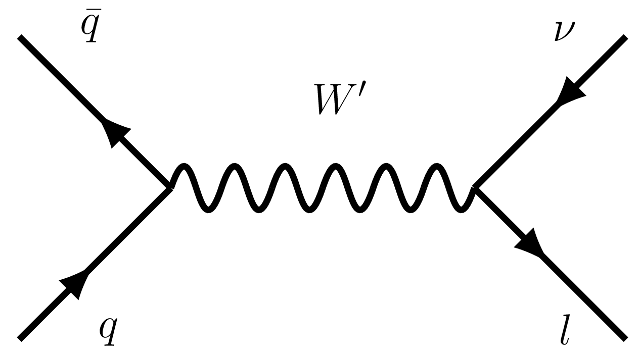
Figure 2.1: $W^{\prime}$ boson contribution to the production of a lepton and a neutrino in $q\bar{q}$ scattering.

The missing transverse energy $E\!\!\!/_{T}$ is evaluated by the vector sum of the transverse momenta of the following components: leptons, photons, and jets. Table 2.2.1 and Table 2.2.1 show the summary for these object selections and isolation criteria, respectively.

Object selections Object $E^{e}_{T}(p^{\mu,jet}_{T})$ $\left|\eta\right|$ Identification $e$ 0 0 $>65\,$ GeV 0 $<1.37,\,[1.52,2.47]$ tight identification $\mu$ 0 0 $>55\,$ GeV 0 $[0.1,1.01],\,[1.1,2.4]$ high-$p_{T}$ identification jet 0 0 $>20\,$ GeV 0 $<2.4$ - 0 $>30\,$ GeV 0 $[2.4,2.5]$ -

Isolation criteria Object Calorimeter isolation Track isolation $\Delta R$ $e$ 0 0 $E^{cone20}_{T}/p_{T}\,<\,0.06$ 0 $p^{cone20}_{T}/p_{T}\,<\,0.06$ $0.2$ $\mu$ 0 0 - 0$p^{cone30}_{T}/p_{T}\,<\,0.15$ $\min(10\,GeV/p_{T},0.3)$ for $p_{T}>1\,GeV$

2.2.2 Event selection

The missing transverse energy ($E\!\!\!/_{T}$) and the transverse mass ($m_{T}$) observables are used to select events from the electron and muon channels. Here, $m_{T}(l,E\!\!\!/_{T})$ can be calculated by following formula,

$$m_{T}(l,E\!\!\!/_{T})=\sqrt{2\,p^{l}_{T}E\!\!\!/_{T}\left(1-\cos\phi_{l\nu}\right)}~{},$$ (2.1)

where $p^{l}_{T}$ is the lepton transverse momentum, and $\phi_{l\nu}$ refers the azimuthal angle difference between the lepton and missing energy momenta.

For the electron channel, each event must have exactly one electron satisfying the conditions stated in Section 2.2.1. Any events containing additional electrons or muons with $p_{T}>20\,{\rm GeV}$ are vetoed. Events are then required to satisfy $E\!\!\!/_{T}>65\,{\rm GeV}$ and $m_{T}(e,E\!\!\!/_{T})>130\,{\rm GeV}$.

For the muon channel, there must be exactly one muon passing the selections listed in Section 2.2.1. Events are vetoed if they feature electrons that satisfy both $p_{T}>20\,{\rm GeV}$ and $\Delta R(e,\mu)>0.1$. Events including any additional muons with $p_{T}>20\,{\rm GeV}$ are also vetoed. The missing transverse energy and the transverse mass must satisfy $E\!\!\!/_{T}>55\,{\rm GeV}$ and $m_{T}(\mu,E\!\!\!/_{T})>110\,{\rm GeV}$.

2.3 Validation

2.3.1 Event generation

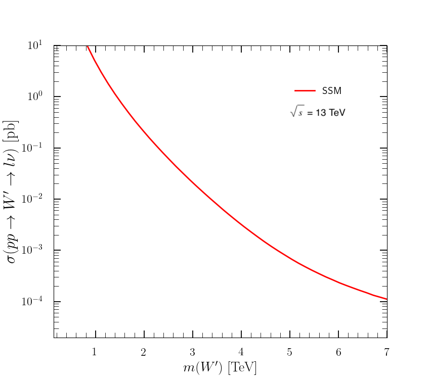
Figure 2.2: Cross-sections for $W^{\prime}$ production and its decay into one lepton-neutrino pair, at leading order and at $\sqrt{s}=13\,{\rm TeV}$ as a function of $W^{\prime}$ mass.

The SSM with heavy gauge bosons has been implemented in the FeynRules package[45], from which UFO model files have been generated. They are then imported into MadGraph5_aMC@NLO[46] to generate the signal samples relevant for the validation of our re-implementation. In the SSM simplified model set-up, we switch off all $W^{\prime}$ couplings to right-handed SM fermions ($\kappa_{R}=0$ in the model conventions), and set the couplings to the left-handed SM fermions to be the same as those of the SM $W$ boson ($\kappa_{L}=1$ in the model conventions). The decay width of the $W^{\prime}$ boson is finally automatically determined by its mass and couplings to fermions within MadGraph5_aMC@NLO by means of MadSpin[47] and MadWidth[48].

Signal events describing the $pp\rightarrow W^{\prime}\rightarrow l\,\nu_{l}$ ($l\,=\,e,\,\mu$) process are generated. Both on-shell and off-shell heavy gauge boson contributions are included. The interference between the SM contributions and the SSM ones is, however, not considered, since the SM $W$ bosons are mostly produced almost on-shell and the mass gap between the $W$ and $W^{\prime}$ bosons is much larger than their decay widths. Signal events with various $W^{\prime}$ masses are generated by MadGraph5_aMC@NLO v$2.6.7$[46] at leading order (LO), with the LO set of NNPDF $2.3$ parton densities with $\alpha_{s}(m_{Z})=0.130$ [49], as obtained from LHAPDF6[50]. We use Pythia 8.224[51] for parton showering and hadronisation.

The following commands were used to generate events in MadGraph5_aMC @NLO.

$$\begin{split}&\tt import\ model\ WEff\_UFO\\ &\tt define\ p\ =\ g\ u\ c\ d\ s\ u\sim\ c\sim\ d\sim\ s\sim\\ &\tt define\ l+\ =\ e+\ mu+\\ &\tt define\ l-\ =\ e-\ mu-\\ &\tt define\ vl\ =\ ve\ vm\ vt\\ &\tt define\ vl\sim\ =\ ve\sim\ vm\sim\ vt\sim\\ &\tt generate\ p\ p\ >\ wp-\ >\ l-\ vl\sim\\ &\tt add\ process\ p\ p\ >\ wp+\ >\ l+\ vl\\ &\tt output\end{split}$$ (2.2)

In the param_card file, kr and kl are set to $0$ and $1$ respectively, and the $W^{\prime}$ mass MWP varies from 2 TeV to 6 TeV with its decay width being automatically calculated. In the run_card file, both fixed_ren_scale and fixed_fac_scale are set to False, and thus the QCD renormalization and collinear factorization scales are set to the averaged transverse mass of the final state particles. Half a million signal events are generated for each mass point. The corresponding cross-sections estimated by MadGraph5_aMC@NLO for various $W^{\prime}$ masses are shown in Fig. 2.2. For a mass of $2(6)\,{\rm TeV}$ for example, we obtain the cross-sections of $195(0.238)\,{\rm fb}$. Overall, the cross-sections are in agreement with those from Fig. 2 in the considered ATLAS paper[14].

Comparison of MadAnalysis 5 and ATLAS predictions for the $m_{T}$-spectrum in the electron channel ($W^{\prime}\rightarrow e\,\nu$). The overflow bins are not accounted for. The relative differences ($\delta$) between our ratios ($R^{MA5}$) and those of ATLAS ($R^{ATLAS}$) are calculated by eq. (2.3). $W^{\prime}$ mass $m_{T}$ range(${\rm GeV}$) $130-400$ $400-600$ $600-1000$ $1000-2000$ $2000-3000$ $3000-10000$ $R^{ATLAS}$ $0.0341\pm 0.0019$ $0.0428\pm 0.0029$ $0.130\pm 0.009$ $0.725\pm 0.046$ $0.0672\pm 0.0175$ $0.000190\pm 0.000017$ $2\,{\rm TeV}$ $R^{MA5}$ $0.0329$ $0.0429$ $0.134$ $0.726$ $0.0644$ $0.000173$ difference($\%$) $3.50$ $0.148$ $2.75$ $0.0468$ $4.12$ $9.25$ $R^{ATLAS}$ $0.0415\pm 0.0017$ $0.0355\pm 0.0019$ $0.0770\pm 0.0049$ $0.272\pm 0.016$ $0.522\pm 0.029$ $0.0528\pm 0.0140$ $3\,{\rm TeV}$ $R^{MA5}$ $0.0409$ $0.0345$ $0.0779$ $0.273$ $0.521$ $0.0530$ difference($\%$) $1.50$ $2.86$ $1.15$ $0.423$ $0.114$ $0.377$ $R^{ATLAS}$ $0.0836\pm 0.0028$ $0.0563\pm 0.0025$ $0.0943\pm 0.0052$ $0.189\pm 0.010$ $0.210\pm 0.011$ $0.367\pm 0.019$ $4\,{\rm TeV}$ $R^{MA5}$ $0.0812$ $0.0566$ $0.0875$ $0.182$ $0.212$ $0.381$ difference($\%$) $2.86$ $0.503$ $7.24$ $3.46$ $0.786$ $3.77$ $R^{ATLAS}$ $0.159\pm 0.005$ $0.101\pm 0.004$ $0.147\pm 0.008$ $0.200\pm 0.011$ $0.118\pm 0.006$ $0.275\pm 0.015$ $5\,{\rm TeV}$ $R^{MA5}$ $0.159$ $0.0955$ $0.136$ $0.185$ $0.119$ $0.306$ difference($\%$) $0.0985$ $5.44$ $7.69$ $7.63$ $1.25$ $11.1$ $R^{ATLAS}$ $0.226\pm 0.007$ $0.141\pm 0.005$ $0.197\pm 0.010$ $0.230\pm 0.012$ $0.0848\pm 0.0045$ $0.121\pm 0.006$ $6{\rm TeV}$ $R^{MA5}$ $0.230$ $0.135$ $0.186$ $0.213$ $0.0844$ $0.151$ difference($\%$) $1.76$ $4.26$ $5.55$ $7.22$ $0.464$ $24.8$

Same as in Table 2.3.1, but for the muon channel ($W^{\prime}\rightarrow\mu\,\nu$) $W^{\prime}$mass $m_{T}$ range(${\rm GeV}$) $110-400$ $400-600$ $600-1000$ $1000-2000$ $2000-3000$ $3000-10000$ $R^{ATLAS}$ $0.0443\pm 0.0026$ $0.0537\pm 0.0036$ $0.152\pm 0.011$ $0.606\pm 0.054$ $0.138\pm 0.020$ $0.00633\pm 0.00453$ $2\,{\rm TeV}$ $R^{MA5}$ $0.0416$ $0.0547$ $0.165$ $0.608$ $0.128$ $0.00368$ difference($\%$) $6.21$ $1.81$ $8.47$ $0.246$ $7.23$ $41.9$ $R^{ATLAS}$ $0.0544\pm 0.0039$ $0.0426\pm 0.0033$ $0.0955\pm 0.0085$ $0.302\pm 0.035$ $0.356\pm 0.053$ $0.150\pm 0.039$ $3\,{\rm TeV}$ $R^{MA5}$ $0.0491$ $0.0427$ $0.104$ $0.348$ $0.328$ $0.128$ difference($\%$) $9.84$ $0.112$ $9.05$ $15.3$ $7.745$ $14.6$ $R^{ATLAS}$ $0.107\pm 0.010$ $0.0634\pm 0.0064$ $0.105\pm 0.011$ $0.212\pm 0.030$ $0.224\pm 0.039$ $0.289\pm 0.090$ $4\,{\rm TeV}$ $R^{MA5}$ $0.0994$ $0.0610$ $0.109$ $0.240$ $0.241$ $0.250$ difference($\%$) $7.21$ $3.73$ $3.83$ $13.2$ $7.78$ $13.6$ $R^{ATLAS}$ $0.198\pm 0.015$ $0.108\pm 0.009$ $0.152\pm 0.013$ $0.204\pm 0.023$ $0.119\pm 0.020$ $0.219\pm 0.072$ $5\,{\rm TeV}$ $R^{MA5}$ $0.184$ $0.103$ $0.150$ $0.210$ $0.140$ $0.212$ difference($\%$) $6.86$ $4.45$ $1.21$ $3.01$ $18.1$ $3.38$ $R^{ATLAS}$ $0.272\pm 0.012$ $0.146\pm 0.008$ $0.194\pm 0.011$ $0.215\pm 0.017$ $0.0771\pm 0.0109$ $0.0954\pm 0.309$ $6\,{\rm TeV}$ $R^{MA5}$ $0.262$ $0.145$ $0.194$ $0.217$ $0.0803$ $0.103$ difference($\%$) $3.67$ $1.15$ $0.419$ $1.02$ $4.14$ $7.43$

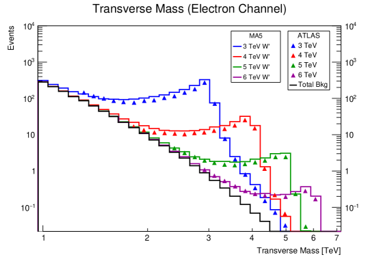
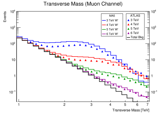
Figure 2.3: $m_{T}$-distributions in the electron channel and muon channel. The solid lines represent our signal predictions for each $W^{\prime}$ mass in MA5, and the triangle dots represent those of ATLAS.

2.3.2 Comparison with ATLAS result for a luminosity of $139\,{\rm fb}^{-1}$

In the absence of any official ATLAS cutflow in Ref. [14], we decided to validate our implementation by comparing the $m_{T}$-distributions of our $W^{\prime}$ signal events after all cuts with those of ATLAS. Here, $m_{T}$ refers to the transverse mass of the system comprising the signal lepton and the missing momentum.

In Table 2.3.1 (Table 2.3.1), we present the comparison of $m_{T}$-distributions for $m_{T}$ values ranging from $130$ $(110)\,{\rm GeV}$ to $10\,{\rm TeV}$ in the electron (muon) channel between our MadAnalysis 5 (MA5) results and the ATLAS official results. For each $W^{\prime}$ mass, there are six signal regions defined according to their $m_{T}$ ranges. We define the relative differences ($\delta$) between MA5 predictions and ATLAS official estimates as below,

$$\delta=\frac{\left|R^{ATLAS}-R^{MA5}\right|}{R^{ATLAS}}\times 100[\%]$$ (2.3)

where $R^{MA5}$ and $R^{ATLAS}$ refer to the ratio of the number of events in each region over the total number of events for each $W^{\prime}$ mass, for our analysis and for ATLAS study respectively. The relative differences $(\delta)$ are up to $20\%$ or within the uncertainty range given by ATLAS in most signal regions. In the electron channel, the differences are all below $10\%$ except for $24.8\%$ for the [3, 10] TeV bin. In the muon channel, for regions of $m_{T}$ below 1 TeV, the differences are all under $10\%$, while some differences reach up to around $15\%$ for those over 1 TeV. There is one $m_{T}$-region whose relative difference far exceeds $20\%$ — when the transverse mass lies in the $[3,10]\,{\rm TeV}$ window for scenarios in which 2 ${\rm TeV}$ $W^{\prime}$ boson decays into a muon-neutrino pair. However, this huge discrepancy can be well resolved when considering the large uncertainty associated with this region that is reported by the ATLAS collaboration. Therefore, we confirm that our reimplementation predictions are in good agreement with the official ATLAS results.

Fig. 2.3 shows the transverse mass distributions with $W^{\prime}$ masses varying from 3 ${\rm TeV}$ to 6 ${\rm TeV}$. The signal predictions of our MadAnalysis 5 implementation as well as those from ATLAS are stacked on top of the total background extracted from the official ATLAS results[14]. In both the electron and muon channels, we obtain a good agreement between the figures of our reimplementation and the original analysis[14].

2.4 Conclusions

We have presented the reimplementation of the heavy charged gauge boson search ATLAS-EXOT-2018-30 [14] in the MadAnalysis 5 framework. Samples of signal events describing the $pp\rightarrow W^{\prime}\rightarrow l\,\nu_{l}$ ($l$ = $e$ or $\mu$) process at $\sqrt{s}=13\,{\rm TeV}$ in the sequential standard model have been generated with MadGraph5_aMC@NLO at LO, and the simulation of the ATLAS detector has been achieved with Delphes 3. We have compared predictions made by MadAnalysis 5 with the results provided by the ATLAS collaboration. We have considered various benchmark scenarios in both the electron and the muon channel, where a good agreement at the level of $m_{T}$ spectra is achieved between our reinterpretation and ATLAS results. Relative differences of at most 20% have been observed, with the most extreme discrepancy being well explained by the large uncertainty populating the corresponding signal region.

The material that has been used for the validation of this implementation is available, together with the MadAnalysis 5 C++ code, at the MA5 dataverse (https://doi.org/10.14428/DVN/GLWLTF) [15].

Acknowledgments

We are very grateful to the ATLAS EXOT conveners for their help and all the additional information they provided, and to Magnar Bugge in particular who were invaluable in our validation process. We would also like to express our sincere gratitude to all the tutors at the second MadAnalysis 5 workshop on LHC recasting.

3 Implementation of the CMS-EXO-17-015 analysis (leptoquark and dark matter with one muon, one jet and missing transverse energy; 77.4 fb^-1)

By Benjamin Fuks and Adil Jueid

3.1 Introduction

Since the discovery of the Higgs boson, the Standard Model (SM) of particle physics is considered to be a good low energy approximation of a more complete, yet undiscovered, theoretical framework. Such a theoretical framework may in particular be able to address questions such as the nature of dark matter (DM) in the universe, among many other interesting issues. Unfortunately, only little is known about the true nature of DM, despite the extensive searches carried out both in laboratories and astrophysical experiments.

At the LHC, one of the most known of and used strategies consists of looking for the presence of a significant excess in the tail of the missing transverse energy ($|$$\vec{p}_{\textrm{miss}}$$|$) distribution. A specific emphasis is put on a signature comprised of dark matter particles recoiling against a visible hard SM object like a photon, a jet, an electroweak gauge boson or even an SM Higgs boson or a top quark [52, 53, 54, 55, 56, 57, 58, 59]. Multiple associated searches have been conducted by the ATLAS and the CMS collaborations, the most recent ones analysing data recorded during the LHC Run 2 [60, 61, 62, 63, 64, 65, 66, 67, 68, 69, 70, 71, 72, 73, 74, 75, 76, 77, 78, 79, 80, 81, 82]. Consequently to the absence of direct evidence for the existence of DM so far, these results have been used to severely constrain the DM couplings and masses in large classes of new physics scenarios. In particular, the absence of any DM signal at the LHC in the so-called thermal freeze-out mechanism has called for either going beyond standard freeze-out, or investigating alternative models.

One of the most attractive of those contexts is the so-called co-annihilation paradigm in which DM is produced in association with beyond-the-SM partners very close in mass. In the framework developed in Ref. [83], the SM field content is extended by a scalar leptoquark doublet $M_{s}$, a weak doublet of Dirac fermions $X$ and a Majorana fermion $\chi$ that plays the role of dark matter. These new states have the following assignments under the SM gauge group $SU(3)_{c}\otimes SU(2)_{L}\otimes U(1)_{Y}$,

$$M_{s}\equiv\begin{pmatrix}M^{u}_{s}\\ M^{d}_{s}\end{pmatrix}:({\bf 3},{\bf 2},7/3)\qquad X\equiv\begin{pmatrix}X_{u}\\ X_{d}\end{pmatrix}:({\bf 3},{\bf 2},7/3),\qquad\chi:({\bf 1},{\bf 1},0),$$ (3.1)

and the relevant interaction Lagrangian ${\cal L}_{\rm NP}$ can be written as

$$\mathcal{L}_{\rm NP}=-\left(y_{D}\overline{X}M_{s}\chi+y_{Q\ell}\overline{Q}_{L}M_{s}\ell_{R}+y_{Lu}\overline{L}_{L}M_{s}^{c}u_{R}+\textrm{h.c.}\right).$$ (3.2)

In parallel, the LHC collaborations developed search strategies dedicated to this class of models. The CMS-EXO-17-015 analysis [16] considered in this proceedings contribution is one of these. In this analysis, the CMS collaboration has focused on one of the benchmarks detailed in Ref. [83]. It assumes that $y_{Lu}=0$, and the other model parameters are chosen as

$$y_{Q\ell}=\sqrt{2}/10,~{}y_{D}=0.1,~{}~{}\Delta=\frac{M_{X}-m_{\chi}}{m_{\chi}}=0.1.$$ (3.3)

In this note, we report on the implementation of this CMS-EXO-17-015 analysis in the MadAnalysis 5 framework [6, 7, 3, 8, 84]. The relevant code for the MadAnalysis 5  implementation can be found in https://doi.org/10.14428/DVN/ICOXG9. In Sec. 3.2, we describe the analysis that we implemented, including a detailed description of the object definitions and event selection strategy. We discuss the validation of our implementation, focusing both on the Monte Carlo event generation necessary for this task and on a comparison of the MadAnalysis 5 predictions with the official CMS results, in Sec. 3.3. We summarise our work in Sec. 3.4.

3.2 Description of the analysis

In the considered theoretical framework, leptoquark (LQ) pair production and decay lead to several signatures, their respective relevance depending on the LQ branching ratios. In the CMS-EXO-17-015 analysis, the final state under consideration is comprised of one isolated muon, one jet and a large amount of missing transverse energy. This process is illustrated by the Feynman diagram shown in Fig. 3.1.

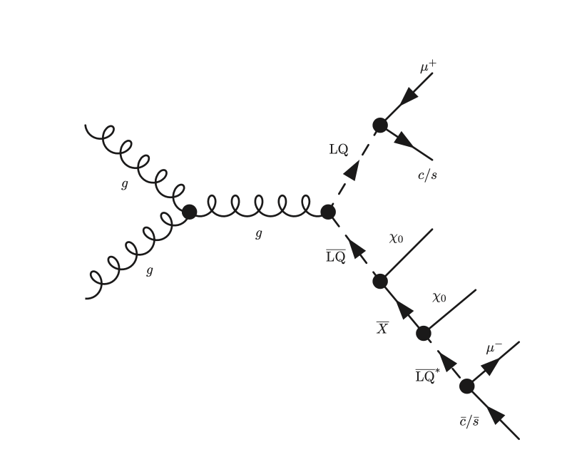
Figure 3.1: Representative parton-level Feynman diagram illustrating the class of processes probed by the CMS-EXO-17-015 analysis.

3.2.1 Object definitions

As above-mentioned, the considered analysis relies on the presence of hard final-state jets and muons, as well as on the one of a large amount of missing transverse energy. In addition, a veto is imposed on the presence of final-state objects of a different nature.

Candidate muons (the leading one being assumed to originate from the decay of a LQ, as illustrated by the Feynman diagram of Fig. 3.1) are required to satisfy tight selection criteria [85]. Moreover, their transverse momentum $p_{T}^{\mu}$ and pseudorapidity $\eta^{\mu}$ must fulfil

$$p_{T}^{\mu}>60~{}\textrm{GeV},~{}\textrm{and}~{}|\eta^{\mu}|<2.4.$$ (3.4)

In addition, those muons are enforced to be isolated to suppress any potential contribution of muons arising from hadronic decays. This relies on an isolation variable $I$ defined by

$$I\equiv\frac{1}{p_{T}^{\mu}}\sum_{i}p_{T,i},$$ (3.5)

with the sum running over all photon, neutral hadron and charged hadron candidates reconstructed within a distance, in the transverse plane, of $\Delta R\equiv\sqrt{(\Delta\eta)^{2}+(\Delta\phi)^{2}}=0.4$ around the muon direction. This isolation variable is required to satisfy $I<0.15$. On the other hand, the analysis also makes use of loose muons to reduce the contribution of $Z$+jets background events (see below). Those are required to satisfy $I<0.25$ and $p_{T}^{\mu}>10~{}\textrm{GeV}$.

Reconstructed electron candidates are required to have a transverse momentum $p_{T}^{e}>15~{}\textrm{GeV}$ and a pseudorapidity $|\eta^{e}|<2.5$. Moreover, they are considered only if they satisfy loose identification criteria [86]. Hadronically decaying tau leptons ($\tau_{h}$) are also identified through loose criteria [87], their selection additionally enforcing $p_{T}^{\tau}>20~{}\textrm{GeV}~{}~{}|\eta^{\tau}|<2.3$.

Jets are reconstructed by means of the anti-$k_{T}$ algorithm [42], with a radius parameter $R=0.4$. The signal jet collection is then comprised of all jets whose pseudorapidity satisfies $|\eta^{j}|<2.4$. The Combined Secondary Vertex (CSVv2) algorithm is then used to identify the jets originating from the fragmentation of a $b$-quark, the analysis making use of its tight working point [88]. The corresponding $b$-tagging efficiency is given by

$$\mathcal{E}_{b|b}(p_{T})=\begin{cases}-0.033+0.0225~{}p_{T}-3.5\!\cdot\!10^{-4}~{}p_{T}^{2}+2.586\!\cdot\!10^{-6}~{}p_{T}^{3}-9.096\!\cdot\!10^{-9}~{}p_{T}^{4}\\ \quad+1.212\!\cdot\!10^{-11}~{}p_{T}^{5}\quad\ \ \textrm{ for }~{}20~{}\textrm{GeV}<p_{T}\leqslant 50~{}\textrm{GeV}\ ,\\[4.0pt] 0.169+0.013~{}p_{T}-1.9\!\cdot\!10^{-4}~{}p_{T}^{2}+1.373\!\cdot\!10^{-6}~{}p_{T}^{3}-4.923\!\cdot\!10^{-9}~{}p_{T}^{4}\\ \quad+6.87\!\cdot\!10^{-12}~{}p_{T}^{5}\quad\ \ \textrm{ for }~{}50~{}\textrm{GeV}<p_{T}\leqslant 160~{}\textrm{GeV}\ ,\\[4.0pt] 0.62-8.3\!\cdot\!10^{-4}~{}p_{T}+4.3078\!\cdot\!10^{-7}~{}p_{T}^{2}\\ \quad\ \ \textrm{ for }~{}160~{}\textrm{GeV}<p_{T}\leqslant 1000~{}\textrm{GeV},\end{cases}$$ (3.6)

while the associated mistagging probabilities of a charmed jet ($\mathcal{E}_{c|b}$) and a light jet ($\mathcal{E}_{j|b}$) as a $b$-jet are given by

$$\begin{split}\mathcal{E}_{c|b}(p_{T})=&\begin{cases}0.0234-8.417\!\cdot\!10^{-5}~{}p_{T}+1.24\!\cdot\!10^{-6}~{}p_{T}^{2}-5.5\!\cdot\!10^{-9}~{}p_{T}^{3}+9.96\!\cdot\!10^{-12}~{}p_{T}^{4}\\ -6.32\!\cdot\!10^{-15}~{}p_{T}^{5}\quad\ \textrm{ for }~{}20~{}\textrm{GeV}<p_{T}\leqslant 65~{}\textrm{GeV}\ ,\\[4.0pt] 0.0218+2.46\!\cdot\!10^{-5}~{}p_{T}-2.021\!\cdot\!10^{-8}~{}p_{T}^{2}\\ \quad\ \textrm{ for }~{}65~{}\textrm{GeV}<p_{T}\leqslant 1000~{}\textrm{GeV},\end{cases}\\ \mathcal{E}_{j|b}(p_{T})=&\begin{cases}0.00284-8.63\!\cdot\!10^{-5}~{}p_{T}+1.38\!\cdot\!10^{-6}~{}p_{T}^{2}-9.69\!\cdot\!10^{-9}~{}p_{T}^{3}+3.19\!\cdot\!10^{-11}~{}p_{T}^{4}\\ -3.97\!\cdot\!10^{-14}~{}p_{T}^{5}\quad\ \textrm{ for }~{}20~{}\textrm{GeV}<p_{T}\leqslant 150~{}\textrm{GeV},\\[4.0pt] 6.3\!\cdot\!10^{-4}+4.51\!\cdot\!10^{-6}~{}p_{T}+2.83\!\cdot\!10^{-9}~{}p_{T}^{2}\\ \quad\ \textrm{ for }150~{}\textrm{GeV}<p_{T}\leqslant 1000~{}\textrm{GeV}.\end{cases}\end{split}$$ (3.7)

Finally, one defines the missing transverse energy as the magnitude of the transverse momentum imbalance ($\vec{p}_{\textrm{miss}}$), which is computed as the opposite of the vectorial sum of the transverse momentum of all reconstructed objects,

$$\vec{p}_{\textrm{miss}}=-\left[\sum_{\textrm{electrons}}\vec{p}_{T}+\sum_{\textrm{muons}}\vec{p}_{T}+\sum_{\textrm{photons}}\vec{p}_{T}+\sum_{\textrm{hadrons}}\vec{p}_{T}\right].$$

In our simulation setup, we have implemented the above parametrisations in a customized Delphes 3 card that has then been used for the simulation of the CMS detector response.

3.2.2 Event selection

The CMS-EXO-17-015 event selection strategy includes two stages, namely a preselection and the definition of a signal region that we coin, in the following, SignalRegion.

In the preselection procedure, events are first selected by requiring the presence of at least one tightly isolated muon with $p_{T}>60~{}\textrm{GeV}$ and $|\eta|<2.4$. The leading jet is then required to satisfy $p_{T}>100~{}\textrm{GeV}$ and to be separated from the leading muon in the transverse plane by $\Delta R>0.5$. Events satisfying those criteria are assumed to be compatible with the production of a leptoquark that decays into those leading jet and muon.

As a next step, several vetoes are applied to reduce the contamination of the overwhelming $t\bar{t}$, $W+$ jets and $Z+$ jets backgrounds. First, events are vetoed if at least one $b$-tagged jet is present. Moreover, a veto on events featuring either a loose electron candidate or a hadronic tau candidate is applied. These three vetoes are necessary to jointly suppress the $t\bar{t}$ background, while the electron and tau vetoes specifically suppress the $W/Z+$ jets contributions.

Next, the transverse mass ($m_{T}$) of the system comprised of the leading muon and the missing momentum is used to further suppress the $W+$ jets background: One imposes that $m_{T}>100~{}\textrm{GeV}$. In addition, the contribution of the $Z+$ jets background is further reduced by rejecting events that contain one extra loosely identified muon candidate with an electric charge that is opposite to the one of the leading muon, and for which

$$|m_{\mu\mu}-M_{Z}|<10~{}\textrm{GeV}.$$ (3.8)

In this expression, $m_{\mu\mu}$ stands for the invariant mass of the system comprised of this muon and the leading muon, such a system being thus constrained to be incompatible with the decay of an on-shell $Z$-boson, if present in the event final state.

Finally, the preselection ends by an extra requirement on the missing momentum $\vec{p}_{\textrm{miss}}$ that is enforced to be well separated in azimuth from the leading jet and the leading muon. We require

$$\Delta\phi(\textrm{jet},\vec{p}_{\textrm{miss}})>0.5~{}~{}\Delta\phi(\mu,\vec{p}_{\textrm{miss}})>0.5,$$ (3.9)

with $\Delta\phi(i,j)=|\phi_{i}-\phi_{j}|$. Whereas these last requirements have very minor effects on the considered signal, they allow in particular for the suppression of the multijet background. For this reason, while implemented in our recasting code, they will be absent from the cut-flow tables presented in the next section.

After this preselection, the signal region is defined by a more stringent cut on the $m_{T}$ variable,

$$m_{T}>500~{}\textrm{GeV}.$$ (3.10)

A summary of the full set of selection cuts is presented in table 3.2.2.

Selection cuts defining the unique CMS-EXO-17-015 signal region. The first column introduces our naming scheme for each cut, as used in the cut-flow tables presented in the next section.        Basic requirements SignalMuon At least one isolated muon with $p_{T}>60~{}\textrm{GeV}$ and $|\eta|<2.4$. SignalJet The leading jet should fulfil $p_{T}>100~{}\textrm{GeV}$, $|\eta|<2.4$ and be separated by $\Delta R>0.5$ from the leading muon.        Vetoes $b$-Veto Veto of events featuring at least one $b$-jet with $p_{T}>30~{}\textrm{GeV}$ and $|\eta|<2.4$. tau-Veto Veto of events featuring at least one hadronic tau with $p_{T}>20~{}\textrm{GeV}$ and $|\eta|<2.3$. $e$-Veto Veto of events featuring at least one loosely reconstructed electron with $p_{T}>15~{}\textrm{GeV}$ and $|\eta|<2.4$.        Further preselection requirements ZMassWindow No extra loose muon that could arise, together with the leading muon, from a $Z$-boson decay (i.e. if $|m_{\mu\mu}-M_{Z}|<10~{}\textrm{GeV}$). $\vec{p}_{\textrm{miss}}$-threshold $|\vec{p}_{\textrm{miss}}|>100~{}\textrm{GeV}$. $m_{T}$-threshold The transverse mass of the muon-$\vec{p}_{\textrm{miss}}$ system must fulfil $m_{T}>100~{}\textrm{GeV}$.        Signal region SignalRegion Extra $m_{T}$ requirement: $m_{T}>500~{}\textrm{GeV}$.

3.3 Validation

3.3.1 Event generation

For the validation of our implementation of the CMS-EXO-17-015 analysis, we generate events describing the dynamics of the signal of Fig. 3.1 in the context of the model introduced in Sec. 3.1. We use MadGraph5_aMC@NLO [46] to simulate hard-scattering events at the leading order (LO) in the strong coupling, excluding the potentially relevant $t$-channel leptonic exchange diagrams [89]. In our procedure, we convolute the LO matrix elements with the LO set of NNPDF 3.0 parton distribution functions in the four-flavour-number scheme, and with $\alpha_{s}(M_{Z})=0.130$. Moreover, we set the renormalisation and factorisation scales to the average transverse mass of the final-state objects.

We use Pythia 8  (version 8.432) [51] to match the fixed-order results with parton showers and to deal with the hadronisation of the resulting partons, after ignoring multi-parton interactions. The response of the CMS detector is then modeled by means of the fast detector simulation toolkit Delphes 3 (version 3.4.2) [9], that internally relies on FastJet (version 3.3.0) [43] for jet clustering. In this last step, we have designed a customized Delphes 3  parametrisation that accurately matches the actual CMS performance working points of the analysis. This card is available, together with our code, from the MadAnalysis 5 Physics Analysis Database (PAD).

Cut-flow charts associated with the CMS-EXO-17-015 analysis and the process depicted in Fig. 3.1 for the two benchmark scenarios BP1 (upper panel) and BP2 (lower panel). We show results obtained with MadAnalysis 5 (second column) and those provided by the CMS collaboration (third column). The numbers inside brackets correspond to the selection efficiency of each cut and the ratio $\mathcal{R}_{i}$ depicting the differences between our predictions and the official CMS results is defined in Eq. (3.12).         Cut         MadAnalysis 5         CMS         $\mathcal{R}_{i}$         Initial events         $99977~{}(100\%)$         $99977~{}(100\%)$         $0$         SignalMuon         $88583~{}(88.66\%)$         $90104~{}(90.12\%)$         $1.61\times 10^{-2}$         SignalJet         $85594~{}(96.62\%)$         $88100~{}(97.77\%)$         $1.17\times 10^{-2}$         $b$-Veto         $79367~{}(92.72\%)$         $84282~{}(95.66\%)$         $3.07\times 10^{-2}$         $\tau_{h}$-Veto         $75572~{}(95.21\%)$         $83373~{}(98.92\%)$         $3.75\times 10^{-2}$         $e$-Veto         $75534~{}(99.94\%)$         $83175~{}(99.7\%)$         $2.41\times 10^{-3}$         ZMassWindow         $71795~{}(95.05\%)$         $81344~{}(97.79\%)$         $2.80\times 10^{-2}$         $\vec{p}_{\textrm{miss}}$-threshold         $69957~{}(97.44\%)$         $78665~{}(96.71\%)$         $1.71\times 10^{-2}$         $m_{T}$-threshold         $65957~{}(94.29\%)$         $74796~{}(95.08\%)$         $8.30\times 10^{-3}$         SignalRegion         $51151~{}(77.75\%)$         $54849~{}(73.33\%)$         $6.02\times 10^{-2}$                  Cut         MadAnalysis 5         CMS         $\mathcal{R}_{i}$         Initial events         $3996~{}(100\%)$         $3996~{}(100\%)$         $0$         SignalMuon         $3519~{}(88.07\%)$         $3625~{}(90.71\%)$         $2.90\times 10^{-2}$         SignalJet         $3441~{}(97.80\%)$         $3586~{}(98.92\%)$         $1.12\times 10^{-2}$         $b$-Veto         $3185~{}(92.57\%)$         $3433~{}(95.73\%)$         $3.33\times 10^{-2}$         $\tau_{h}$-Veto         $3026~{}(95.01\%)$         $3401~{}(99.06\%)$         $4.08\times 10^{-2}$         $e$-Veto         $3024~{}(99.93\%)$         $3392~{}(99.73\%)$         $2.06\times 10^{-3}$         ZMassWindow         $2936~{}(97.11\%)$         $3327~{}(98.08\%)$         $9.88\times 10^{-3}$         $\vec{p}_{\textrm{miss}}$-threshold         $2897~{}(98.69\%)$         $3277~{}(98.49\%)$         $2.07\times 10^{-3}$         $m_{T}$-threshold         $2678~{}(92.44\%)$         $3160~{}(96.42\%)$         $4.12\times 10^{-2}$         SignalRegion         $2162~{}(80.74\%)$         $2611~{}(82.62\%)$         $2.27\times 10^{-2}$         

For the results presented in the rest of this contribution, we have generated $200,000$ events for two benchmark points BP1 and BP2 defined by

$$\begin{split}\texttt{BP1}:&\quad M_{\textrm{LQ}}=1000~{}\textrm{GeV},~{}~{}m_{\chi}=400~{}\textrm{GeV},\\ \texttt{BP2}:&\quad M_{\textrm{LQ}}=1500~{}\textrm{GeV},~{}~{}m_{\chi}=600~{}\textrm{GeV},\end{split}$$ (3.11)

with the other parameters fixed as in Eq. (3.3). About 102,326 (108,208) events pass all the selection criteria of the CMS analysis in the framework of the BP1 (BP2) scenario.

3.3.2 Results

In order to validate our implementation, we compare predictions obtained with our implementation in MadAnalysis 5 to the official results provided by the CMS collaboration for the two benchmark scenarios BP1 and BP2 defined in Sec. 3.3.1. Our comparison is performed in two stages. First, we study the resulting cut-flow tables. Next, we investigate the shape of the distributions of several key observables.

To quantify the level of agreement between our results and the CMS ones at each selection step of the cut-flow, we introduce a quantity ${\cal R}_{i}$ defined by

$$\mathcal{R}=\bigg{|}1-\frac{\epsilon_{MA5}^{i}}{\epsilon_{CMS}^{i}}\bigg{|},$$ (3.12)

with $\epsilon^{i}$ being the selection efficiency of the $i^{\rm th}$ cut $i$,

$$\epsilon^{i}=\frac{n^{i}}{n^{i-1}}.$$ (3.13)

In this notation, $n_{i-1}$ events survive before the $i^{\rm th}$ cut, and $n_{i}$ events survive after this cut. We present the results in the two panels of table 3.3.1 for the BP1 and BP2 setup respectively, after normalising our results to the same cross section as the one used by the CMS collaboration in their analysis. We obtain an excellent level of agreement, reaching $\mathcal{R}\sim 10^{-3}-10^{-2}$.

Moreover, we confront results at the differential level in Fig. 3.2 for different observables relevant for the considered analysis. An excellent agreement is again found.

Figure 3.2: Normalised distributions for some key kinematical quantities used in the CMS-EXO-17-015 analysis. We show predictions for the scenario BP1 with $M_{\textrm{LQ}}=1000~{}\textrm{GeV}$. The MadAnalysis 5  predictions are shown in red while the CMS ones are given in blue. We consider the hadronic tau multiplicity (upper left), the $b$-jet multiplicity (upper right), the transverse momentum of the leading jet (centre left), the transverse momentum of the leading muon (centre right), the missing transverse energy (lower left) and the transverse mass of the leading muon and missing momentum system (lower right).

3.4 Conclusions

In this note, we have made a detailed description of our implementation of the CMS-EXO-17-015 analysis in the MadAnalysis 5 framework. This analysis can be used in particular to constrain models containing scalar or vector leptoquarks that decay primarily into muons and jets. However, the signal region is not defined by relying on the leptoquark invariant mass (to be reconstructed from the leading muon and jet), so that the analysis can in fact be used to probe any model giving rise to muons, jets and missing transverse energy. For given benchmark scenarios, we have found an excellent agreement between our predictions with MadAnalysis 5 and the official results provided by the CMS collaboration. This validated analysis is available on the public MadAnalysis 5 database and can be found from the MadAnalysis 5 dataverse, at https://doi.org/10.14428/DVN/ICOXG9[17], together with relevant validation material.

Acknowledgments

The authors would like to thank Abdollah Mohammadi for kindly providing official CMS cut-flow tables and for his assistance in understanding the event selection used in the CMS-EXO-17-015 analysis. The work of AJ is sponsored by the National Research Foundation of Korea, Grant No. NRF-2019R1A2C1009419.

4 Implementation of the CMS-EXO-17-030 analysis (pairs of trijet resonasnces)

By Yechan Kang, Jihun Kim, Jin Choi and Soohyun Yun

4.1 Introduction

Events associated with a multijet final state at hadron colliders provide a unique window to investigate various beyond standard model (BSM) physics. Typically, in the Standard Model, pair-produced heavy resonances each decaying into three jets only originate from the production of a pair of hadronically decaying top quarks. Therefore, if a particle heavier than the top quark exists, and manifests itself as a narrow resonance, then one should be able to see a clean high mass resonance peak in multijet invariant mass distributions.

We present the results of the recast of the CMS-EXO-17-030 three-jet analysis[18] which targets pair-produced resonances in proton-proton ($pp$) collisions, in a case where each resonance decays into three quarks. In this search, the RPV SUSY model[90] is used as a benchmark, with a varying gluino mass. This allows for the modeling of high mass resonances pair production, followed by subsequent gluino decays into three jets. Moreover, this leads to a final state comprising six quarks at the parton level. In this model, a new quantum number $R$ is defined as

$$R=(-1)^{2S+3B+L},$$

where $S$ is the spin, $B$ is the baryon number, and $L$ is the lepton number. In this search, we consider a model in which $R$-parity is broken via baryon number violation, so that squarks can decay into two quarks (Fig. 4.1). For our recast implementation and its validation, we follow the interpretation of the experimental analysis and the resonance is assumed to be a gluino.

The analysis is divided into four separate regions depending on the mass of the gluino. It exploits the geometrical event topology to discriminate signal events from background events. In order to improve the sensitivity to a wide range of resonance masses, the analysis includes signal regions that are each dedicated to a specific resonance mass, the associated topology and kinematics of the final-state jet activity. This separation is further necessary to manage the estimation of the background properly. In the low mass regions, the main background comes from top quark decays, whereas it comes from QCD events for the high mass regions. By defining different signal regions depending on the gluino mass, we can handle the background properly with different strategies. To perform the validation of our implementation, we select four benchmark gluino mass points representing each signal region, the gluino mass being respectively set to 200 GeV, 500 GeV, 900 GeV, and 1600 GeV. This enables the direct comparison between the recast and the result of the experimental publication in terms of acceptance and therefore allows us to validate our implementation.

In the rest of this note, we present the recast of the CMS-EXO-17-030 analysis in the MadAnalysis 5 framework [6, 7, 3, 8], which is now available from the Madanalysis 5 Public Analysis Database and the MadAnalysis 5 dataverse [19].

4.2 Description of the analysis

To identify pair-produced high mass resonances decaying into multiple jets in LHC events, the jet ensemble technique[91] is applied. This examines all possible combinatorial triplets that could be formed from a jet collection in each event. As a concrete example, we consider an event including 6 jets. First, we collect every possible set of 3 jets into a triplet. There should be 20 combinations of such triplets, and therefore 10 pairs of triplets in each event. All such triplet pairs and triplets are candidates for pair-produced gluinos and their decay. Then, to discriminate the ‘correct’ triplets (which originate from gluino decays) from wrongly combined triplets, and to reject the QCD background as well, we apply cuts on variables that embed the topology expected from the signal events. The cuts are categorized into three stages and applied step by step: event level, triplet pair level, and triplet level. The definition of each variable and the motivation to use them are described in section 4.2.2 in detail.

4.2.1 Object definitions

Jet candidates are reconstructed using the anti-$k_{T}$ algorithm[42] with a radius parameter $R=\sqrt{(\Delta\phi)^{2}+(\Delta\eta)^{2}}=0.4$. Jets in the detector are required to have a transverse momentum, $p_{T}$, larger than 20 GeV and an absolute value of the pseudorapidity, $|\eta|$, of at most 2.4. This analysis neither considers nor vetoes the presence of other objects like hard leptons or photons, so that their precise definition is irrelevant.

Figure 4.1: Feynman diagram representative of pair-produced gluinos decaying into six jets.

4.2.2 Event selection

Four separate signal regions have been defined to target all possible gluino masses in the range of 200 - 2000 GeV: SR1 (200-400 GeV), SR2 (400-700 GeV), SR3 (700-1200 GeV), and SR4 (1200-2000 GeV). The requirements in each signal region are described below.

First of all, each event is required to contain at least six reconstructed jets. From the entire set of jets, only the six jets with the highest $p_{T}$ are considered. Then four selections based on event-level variables are applied. For the low mass regions targeting gluino masses below 700 GeV, all jets in the event must have a $p_{T}$ larger than 30 GeV and the $H_{T}$ variable, defined as the scalar sum of the $p_{T}$s of all jets, is imposed to be larger than 650 GeV. For the high-mass regions dedicated to gluino masses beyond 700 GeV, the $p_{T}$ of all jets must be larger than 50 GeV and the $H_{T}$ variable must be greater than 900 GeV. Jets are arranged in descending order of $p_{T}$, and the $p_{T}$ of the sixth jet is required to be larger than 40 GeV, 50 GeV, 125 GeV, or 175 GeV for the SR1, SR2, SR3, and SR4 signal region respectively.

To discriminate the signal from the QCD main background and wrongly combined triplets, Dalitz variables are adopted. Dalitz variables are effective discriminants for studying three-body decays. They were initially introduced by Dalitz in kaon to three pions decays[92]. The Dalitz variables for a triplet are defined as

$$\hat{m}(3,2)^{2}_{ij}=\frac{m^{2}_{ij}}{m^{2}_{ijk}+m^{2}_{i}+m^{2}_{j}+m^{2}_{k}},$$

where $m_{i},m_{ij}$ and $m_{ijk}$ are respectively the invariant mass of the individual jet $j_{i}$, of the dijet system made of the jets $j_{i}$ and $j_{j}$, and of the triplet. Here, indices refer to the jets in the triplet, where $i,j,k\in\{1,2,3\}.$ These variables have good discriminating power as follows from our signal topology. In signal events for which a massive particle decays into three quarks, the angular distribution of the jets should be even in the center-of-mass frame. Therefore we expect the Dalitz variable to be close to 1/3 for each jet pair ($m_{ij}$).

By utilizing the above property of Dalitz variables, a new variable called the mass distance squared of a triplet is defined as

$$D^{2}_{[3,2]}=\sum_{i>j}\left(\hat{m}(3,2)_{ij}-\frac{1}{\sqrt{3}}\right)^{2}.$$

This variable must be close to zero for symmetrically decaying signal triplets but deviates from zero for wrongly combined triplets and QCD backgrounds which may exhibit an asymmetric topology.

A generalized Dalitz variable is introduced as an extension of the original Dalitz variable for a six-jet topology, which should be close to $1/20$ in the case of even angular distributions. It is defined from the normalized invariant mass of jet triplets,

$$\hat{m}(6,3)^{2}_{ijk}=\frac{m^{2}_{ijk}}{{4m^{2}_{ijklmn}+6\Sigma_{i}m^{2}_{i}}}.$$

Here, $m_{ijklmn}$ refers to the invariant mass of the leading six jets, where $i,j,k,l,m,n\in\{1,2,3,4,5,6\}.$

Using the generalized Dalitz variables and the $D^{2}_{[3,2]}$ value associated with a triplet, the six-jet distance squared of an event is defined as

$$D^{2}_{[(6,3)+(3,2)]}=\sum_{i<j<k}\bigg{(}\sqrt{\hat{m}(6,3)^{2}_{ijk}+D^{2}_{[3,2]ijk}}-\frac{1}{\sqrt{20}}\bigg{)}^{2}.$$

For signal events, each pair-produced gluino is expected to decay symmetrically, which leads to small values of $D^{2}_{[3,2]}$. Furthermore, each generalized Dalitz variable ($m(6,3)^{2}_{ijk}$) is expected to be close to 1/20. Therefore, signal events are likely to feature $D^{2}_{[(6,3)+(3,2)]}$ close to zero. On the other hand, the events containing triplets originating from QCD multijet production will have an asymmetric angular distribution, and thus have values relatively far from zero. The official analysis has shown that the distribution of $D^{2}_{[(6,3)+(3,2)]}$ for QCD multijet events peaks at a farther point than the gluino events, as expected. The $D^{2}_{[(6,3)+(3,2)]}$ variable is used for the last selection at the event level and is required to be smaller than 1.25, 1.00, 0.9, or 0.75 for the SR1, SR2, SR3, and SR4 signal region respectively.

Furthermore, the masses of two distinct triplets are expected to be symmetric in the case of the signal, as originating from the decay of the same particle. Thus the mass asymmetry defined as

$$A_{m}=\frac{|m_{ijk}-m_{lmn}|}{m_{ijk}+m_{lmn}},$$

where $m_{ijk}$ and $m_{lmn}$ are the masses of the two distinct triplets in a triplet pair, is expected to be closer to zero for the correctly combined triplet pairs in the signal case. The mass asymmetry of a triplet pair is required to be smaller than 0.25 or 0.175 for the SR1 and SR2, or 0.15 for the SR3 and SR4.

Finally, selections at the triplet-level are applied. The variable $\Delta$ of a triplet is defined as the sum of the $p_{T}$ of the jets in the triplet ($|p_{T}|_{ijk}$), after subtracting the triplet invariant mass ($m_{ijk}$):

$$\Delta=|p_{T}|_{ijk}-m_{ijk}.$$

In the official analysis, it has been shown that correctly combined triplets have a constant distribution in the mass vs $p_{T}$ plane, whereas in cases of wrongly combined triplets and QCD backgrounds their $p_{T}$ and mass are proportional to each other. Therefore the $\Delta$ observable has good discriminating power between wrongly combined triplets, QCD backgrounds and correctly combined triplets. This value is required to be larger than 250 GeV, 180 GeV, 20 GeV, or -120 GeV for the SR1, SR2, SR3, and SR4 region respectively. For the very last selection, the mass distance squared of a triplet $(D^{2}_{[3,2]})$ is required to be smaller than 0.05, 0.175, 0.2, or 0.25 for each region.

The actual cuts for each variable for the event, triplet pair, and triplet levels are summarized in table 4.2.2.

Selection criteria Events Triplet Pairs Triplets Region Gluino Mass Jet $p_{T}$ $H_{T}$ $p_{T}(j_{6})$ $D^{2}_{[(6,3)+(3,2)]}$ $A_{m}$ $\Delta$ $D^{2}_{[3,2]}$ 1 200-400 GeV $>$30 GeV $>$650 GeV $>$40 GeV $<$1.25 $<$0.25 $>$250 GeV $<$0.05 2 400-700 GeV $>$30 GeV $>$650 GeV $>$50 GeV $<$1.00 $<$0.175 $>$180 GeV $<$0.175 3 700-1200 GeV $>$50 GeV $>$900 GeV $>$125 GeV $<$0.9 $<$0.15 $>$20 GeV $<$0.2 4 1200-2000 GeV $>$50 GeV $>$900 GeV $>$175 GeV $<$0.75 $<$0.15 $>$-120 GeV $<$0.25

4.3 Validation

4.3.1 Event generation

Simulation of double-trijet resonance events is done by making use of the MadGraph5_aMC@NLO version 2.7.3 Monte Carlo generator[46], using the RPVMSSM_UFO model file[93, 94]. For the parton distribution functions, the LO set of NNPDF3.0[95] parton densities with $\alpha_{s}=0.130$, as implemented in LHAPDF6[50], is used. To avoid any squark contribution to gluino production, all the masses of squarks are set to be 2.5 TeV, and the masses of gluinos are set to be 200, 500, 900, and 1600 GeV to target the signal regions resulting from the cuts described in section 4.2.2. Based on the pair production of gluinos, we used MadSpin[47] and MadWidth[48] without spin correlations to simulate the gluino decays into three jets. We compared the acceptance resulting from the cuts described in the next section, using signal samples with and without spin correlation, and found that there is negligible difference in the final acceptance. Here, we thus present the results without any spin correlation.

After the simulation of the hard-scattering process, Pythia8[51] is used for parton showering and hadronization, followed by Delphes3[9] for the fast simulation of the CMS detector response.

4.3.2 Comparison with the official results

As using combined triplets of jets for the final selection, the analysis suffers from two major backgrounds, irreducible QCD backgrounds and a unique background not originating from a specific physical process: wrongly combined triplets. Since the invariant mass distribution is similar for QCD backgrounds and wrongly combined triplets [18], the CMS collaboration made signal and background fitting templates from those distributions and proceed with signal to background fitting directly to the data to calculate the final signal significance. Therefore, the number of triplets that pass all cuts is used indirectly for the final result. To see how many correct triplets survive in each signal region, the signal acceptance has been defined based on the triplet selection described in section 4.2:

$${\rm Acc.}=\frac{{\rm Number~{}of~{}surviving~{}triplets}}{{\rm Number~{}of~{}generated~{}events}}.$$

Here, the acceptance is defined as the ratio of the number of triplets and the number of total events, and not the number of events passing the selections and the total number of events. We hence collect all possible combinations of triplets out of 6 jets and have 20 triplets (or 10 triplet pairs) per single event. In this analysis, we have cuts at the event level, triplet-pair level, and triplet level.

Since the analysis has a distinctive definition of acceptance based on the number of triplets, one of the major difficulties in using the MadAnalysis 5 framework was the implementation of counting the triplets passing the different cuts in each signal region, as there are diverse triplet-level cut thresholds for each region. In MadAnalysis 5, the framework provides cutflows based on the event selection, which makes it hard to count the number of surviving triplets in each signal region. To overcome this problem, we made four collections of triplets, i.e. one for each signal region, and updated each collection with the different cuts for each signal region. Finally, we multiplied each event weight by the number of triplets (for each region), which makes MadAnalysis 5 generating cutflows on triplet level.

The acceptance numbers officially calculated by CMS are of 0.00024, 0.084, 0.17 for SR1, SR3, and SR4. There is no result provided for SR2. For the purpose of recast, we define the difference as

$${\rm Diff.}=\frac{{\rm Acc.(recast)}-{\rm Acc.(CMS~{}official)}}{{\rm Acc.(CMS~{}official)}}$$

to compare the recast values with the official results.

Comparing with the official results, the recast showed a large discrepancy. Acceptances (differences) we calculated are $6.25\times 10^{-4}(140\%),6.5\times 10^{-1}(674\%)$ and $1.71(906\%)$ for SR1, SR3 and SR4. We found out that many wrongly combined triplets not originating from the same gluino still pass the final selection. Since there is no way to calculate the acceptance of the correctly matched triplets as originally performed through the template fit to the CMS data, we chose an alternative approach, using generator level information to check how many triplets from the same gluino can survive after all cuts. Therefore, we require that the correct triplets should be matched to their mother gluino as

• All jets should be matched to generator level partons within a distance in the transverse plane of $\Delta R(j,q)<0.3$, where $q$ generically stands for $u,c,d,s$ and the corresponding antiparticles.

• Matched partons in a triplet should all be quarks, or all be antiquarks.

• All matched (anti)quarks in the triplet should have the same gluino as their mother.

Here, we required the jets to be matched to their mother gluino using the truth level information. For the purpose of generalization, any recasting analysis that wishes to use the truth information should change the Particle Data Group identifier (PID) of the mother particle. We defined the PID of this mother particle by using the #DEFINE preprocessor method, so the user can change the value of the EXO_17_030_PID variable to any other value relevant for the signal of their interest. Therefore, this implementation can be further tested with various other BSM models that allow resonance with three jet decay signature, e.g. searches based on composite quark model[96] or extra dimensional model[97].

The final acceptances that we obtain, for the considered benchmark scenarios, are of $2.8\times 10^{-4}$, $7.3\times 10^{-2}$, and $1.55\times 10^{-1}$ for the SR1, SR3 and SR4 regions. Our predictions show good agreements with the CMS official results, at the level of 8%, 13%, and 8.8% for the SR1, SR3 and SR4 regions. For the SR2 region, the final acceptance is $1.5\times 10^{-2}$. This value has no comparison target because the official acceptance for the SR2 region has not been provided by the CMS collaboration. Detailed results are provided in tables 4.3.2 and 4.3.2.

Cutflows in the Low-Mass Regions. The initial number of triplets that could be reconstructed from each event is assumed to be 20. All triplets are matched to their mother particle. Since there is no official CMS result for SR2, we did not calculate the difference for that region. Signal Region 1 Signal Region 2 Cut Events Triplets Events Triplets Initial events 400,000 8,000,000 400,000 8,000,000 Njets$\geq$6 231,863 4,637,261 367,491 7,349,821 preselection 148,090 2,961,800 341,054 6,821,079 HT 38,434 768,680 329,561 6,591,218 Sixth jet $p_{T}$ 29,611 592,220 242,511 4,850,220 $D^{2}_{[(6,3)+(3,2)]}$ 23,296 465,920 186,731 3,734,618 $A_{m}$ 3,982 4,630 89,853 118,285 $\Delta$ 187 199 5,534 6,501 $D^{2}_{[3,2]}$ 108 112 5,145 5,995 Acc. 0.028% 1.50% Acc.(CMS official) 0.026% Diff. 8%

Cutflows in the High Mass Region. The initial number of triplets reconstructed from each event is assumed to be 20. All triplets are matched to their mother particle. Signal Region 3 Signal Region 4 Cut Events Triplets Events Triplets Initial events 400,000 8,000,000 400,000 8,000,000 Njets$\geq$6 388,119 7,762,382 394,516 7,890,321 preselection 340,320 6,806,404 373,669 7,473,380 HT 339,303 6,786,064 373,661 7,473,221 Sixth jet $p_{T}$ 120,141 2,402,821 166,877 3,337,540 $D^{2}_{[(6,3)+(3,2)]}$ 100,349 2,006,981 113,436 2,268,721 $A_{m}$ 52,205 72,806 69,080 100,637 $\Delta$ 25,465 31,320 49,767 62,731 $D^{2}_{[3,2]}$ 23,948 29,025 49,309 61,959 Acc. 7.3% 15.5% Acc.(CMS official) 8.4% 17.0% Diff. -13% -8.8%

4.4 Conclusion

A recast of the CMS-EXO-17-030 double-three-jet analysis has been performed within the MadAnalysis 5 framework. To validate our implementation, we choose four gluino RPV SUSY scenario with masses ranging from 200 to 2000 GeV. The four masses that we selected are 200 GeV, 500 GeV, 900 GeV, and 1600 GeV, and represent each signal region. In this note, the event selection is described in detail, and corresponding cutflows for each benchmark point are presented. We exhibit the difficulties that are inherent to the usage of MadAnalysis 5 for the CMS-EXO-17-030 recast, as non-event based acceptance calculations are in order. We moreover explain our method to overcome them. The signal events are simulated under the same condition as for the official CMS result, which corresponds to an integrated luminosity of 35.9 fb^-1 of collisions at a center-of-mass energy of 13 TeV, but with a CMS detector configuration based on Delphes 3. The validation is performed in terms of the acceptance for each signal region. The recast and the official results show good agreement, resulting in differences from a minimum of 8% to a maximum of 13%.

The code is available online from the MadAnalysis 5 dataverse [19], at https://doi.org/10.14428/DVN/GAZACQ, on which we also provide cards that were relevant for the validation of this implementation.

Acknowledgments

We congratulate all our colleagues who have participated in the second MadAnalysis 5 workshop on LHC recasting in Korea and thank the organizers and the tutors of the workshop for their sincere support. In addition, Soohyun Yun is grateful for financial support from Hyundai Motor Chung Mong-Koo Foundation.

5 Implementation of the CMS-EXO-19-002 analysis (physics beyond the Standard Model with multileptons; 137 fb^-1)

By Eric Conte and Robin Ducrocq

5.1 Introduction

In this document, we present the implementation of the CMS-EXO-19-002 analysis [20] in the MadAnalysis 5 framework [6, 7, 3, 8]. It consists of a search for events featuring multiple charged leptons, and relies on an integrated luminosity of $137~{}\textrm{fb}^{-1}$ of LHC proton-proton collisions, with a center-of-mass energy $\sqrt{s}=13~{}\textrm{TeV}$.

In this analysis, two classes of models are targetted, which leads to the definition of two categories of signal regions. These consist of a type-III seesaw model [98] including three heavy fermions mediator $\Sigma^{\pm}$ and $\Sigma^{0}$, and a simple extension of the Standard model, called $t\bar{t}\phi$, with one scalar (or pseudoscalar) $\phi$ that can be produced in association with a top-antitop pair [99, 100]. The type-III seesaw signal under consideration arises from the production and decay of $(\Sigma^{\pm}\Sigma^{0})$ and $(\Sigma^{\pm}\Sigma^{\mp})$ pairs ($\Sigma^{0}\Sigma^{0}$ being neglected) in a multilepton final state. On the other hand, the $t\bar{t}\phi$ process with a $\phi\rightarrow l^{+}l^{-}$ decay induces a signal comprising additional $b$-jets originating from the top decays. The search for such signals is done in three $(3L)$ and four $(4L)$ leptons channels, with extra $b$-jets in the case of the $t\bar{t}\phi$ signal. For the validation of the implementation, we take into account predictions and official results with heavy fermion masses of $m_{\Sigma}=300~{}\textrm{GeV}$ and $m_{\Sigma}=700~{}\textrm{ GeV}$ for the type-III seesaw benchmark, and masses of $m_{\phi}=20~{}\textrm{ GeV}$ ($m_{\phi}=70~{}\textrm{GeV}$) for the scalar (pseudoscalar) $t\bar{t}\phi$ model, as the CMS collaboration only provided material for those cases.

In section 5.2, we describe the selection and the manner in which the analysis is implemented in MadAnalysis 5. In particular, we present all signal regions defined in the CMS paper. Sections 5.3 and 5.4 are devoted to the validation of the implementation of the type-III seesaw and $t\bar{t}\phi$ signal regions respectively. We summarize our main results in section 5.5.

5.2 Description of the analysis

5.2.1 Object definitions

Muons are required to have a transverse momentum $p_{T}>10~{}\textrm{GeV}$ and a pseudorapidity $|\eta|<2.4$. Requirements on the tracking quality are not implemented, as the package Delphes 3 that we use for the fast simulation of the CMS detector [9] is not able to reproduce it. To suppress the background, an isolation criterion is applied on the muons. The corresponding procedure relies on a relative isolation variable, Isol$(l)$, defined as the scalar $p_{T}$ sum of all particle-flow objects in a cone of $\Delta R=0.4$ around the lepton direction and normalized to the lepton $p_{T}$. This variable,

$${\rm Isol}(l)=\frac{1}{p_{T}(l)}\sum_{j\neq l}^{\Delta R<0.4}{p_{T}(j)}\hskip 8.5359pt\textrm{with}\ l\ \textrm{being the lepton and}\ j\ \textrm{any particle flow object},$$ (5.1)

must be smaller than $15\%$. The displacement of the muon track with respect to the primary vertex is also constrained,

$$|d_{z}|<0.1~{}\textrm{cm}\ ,\qquad|d_{xy}|<0.05~{}\textrm{cm}.$$ (5.2)

Electrons are required to have a $p_{T}>10~{}\textrm{GeV}$, and a pseudorapidity $|\eta|<2.5$ that is consistent with the tracking system acceptance. Requirements on the electron shower shape and track quality are not implemented. The relative isolation ratio as been chosen to be smaller than $15\%$, and is calculated with a cone of $\Delta R=0.3$ around the electron. The displacement of the electron track with respect to the primary vertex is also constrained:

• $|d_{z}|<0.1~{}\textrm{cm}$ and $|d_{xy}|<0.05~{}\textrm{cm}$ when the electron is in the eletromagnetic calorimeter (ECAL) barrel acceptance ($|\eta|<1.479$);

• $|d_{z}|<0.2~{}\textrm{cm}$ and $|d_{xy}|<0.1~{}\textrm{cm}$ when electron is in the ECAL barrel endcap ($|\eta|>1.479$).

Finally, electrons that are too close to a muon (possibly due to bremsstrahlung from the muon) must be rejected. It is done by searching if there is a muon track in a cone around the electron track with a radius $\Delta R=0.05$.

Jets are defined by using the anti-$k_{T}$ algorithm [42] with a distance parameter of 0.4, as provided by the FastJet package [44, 43]. They must have a $p_{T}>30~{}\textrm{GeV}$ and a $|\eta|<2.1$. No pile-up simulation has been encapsulated because we assume that pile-up suppression algorithms are good enough to get rid of all related soft contamination. Moreover, all jets which are inside a cone of radius $\Delta R=0.4$ around a selected charged lepton are discarded.

We call ’$b$-jets’ the reconstructed jets originating from $B$-hadrons. The $b$-tagging performance in this CMS analysis corresponds to the medium working point of the DeepCSV algorithm [88], with an efficiency of 60–75% and a misidentification rate of 10% for $c$-quark jets and 1% for lighter jets.

In trilepton events, additional constraints are imposed on the charged leptons in order to reduce misidentified-background contributions. If a charged lepton can be matched which a loose $b$-jet (defined by a jet with $p_{T}$ greater than 10 GeV, $|\eta|\leq 2.5$ and a medium $b$-tag), by using a matching cone of $\Delta R<0.4$ around the lepton, the lepton is rejected. Besides, an additional selection cut based on a tri-dimensional impact parameter is also applied on the leptons. The lack of information relative to this quantity implies that we have not implemented this cut in the recast analysis.

Finally, the missing transverse momentum, noted $MET$ or $p_{T}^{miss}$, is taken as the negative vector sum of all particle-flow objects $p_{T}$.

5.2.2 Common event selection

The trigger requirements imply an online selection of the events. This two-stage selection requires at least one electron or one muon in the event with a large $p_{T}$ value. The first step of the offline selection consists of requiring one leading lepton with a threshold a little bit greater than the online selection threshold, and thus encapsulates the online selection. The $p_{T}$ threshold value used in the offline selection depends on the year of data acquirement. For muons, the threshold is 26 GeV for 2016, 29 GeV for 2017 and goes back to 26 GeV for 2018. For electrons, the threshold is 30 GeV for 2016 and 35 GeV for 2017 and 2018. Considering the integrated luminosity recorded by CMS ($37.80~{}\textrm{fb}^{-1}$ for 2016, $44.98~{}\textrm{fb}^{-1}$ for 2017 and $63.67~{}\textrm{fb}^{-1}$ for 2018), we apply a threshold of 26 GeV for 69% of the events (randomly chosen according to a flat distribution) and 29 GeV for the remaining events. Similarly, an electron threshold of 35 GeV is fixed for 74% of the events and 30 GeV for the remaining events.

We select events with three leptons (electrons or muons) or more. In the case where we have four leptons or more, we only keep the four leading leptons and label those events as “4 leptons” events.

All events containing a lepton pair where the two leptons are distant by $\Delta R<0.4$ are rejected. We also remove events that contain a same-flavor lepton pair (independent of the charge) whose invariant mass is below 12 GeV. These two selection cuts allow us to remove low-mass resonances and final-state radiation background contributions.

In the case of a trilepton event, an additional constraint is applied. If the invariant mass of the three leptons is within the $Z$ mass window ($91\pm 15~{}\textrm{GeV}$), the presence of an opposite-sign same-flavor (OSSF) lepton pair with an invariant mass below 76 GeV yields the rejection of the event. This procedure allows us to remove $Z\rightarrow l^{+}l^{-}\gamma$ background contributions where the photon converts into two additional leptons, with one of which being lost.

5.2.3 Event selection and categorization devoted to the type-III seesaw signal

The events are categorised in 7 signal regions according to:

• the number of selected leptons (three or four leptons) in the event,

• the number of opposite-sign same-flavor lepton pairs (OSSF multiplicity),

• the value of the invariant mass of the OSSF lepton pair relative to the $Z$ mass window ($91\pm 15~{}\textrm{GeV}$). If there are several OSSF pairs, the considered invariant mass is the one which is the closest to the $Z$ nominal mass. We refer the three cases as below-Z, on-Z and above-Z.

Table 5.2.3 collects the definition of the different signal regions.

List of the signal regions dedicated to probing the type-III seesaw model. Label $N_{l}$ $N_{OSSF}$ $M_{OSSF}$ additional cut 3L below-Z 3 1 $<76~{}\textrm{GeV}$ - 3L on-Z 3 1 $\in[76;106]$ GeV MET $>$ 100 GeV 3L above-Z 3 1 $>106~{}\textrm{GeV}$ - 3L OSSF0 3 0 - - 4L OSSF0 $\geq 4$ 0 - - 4L OSSF1 $\geq 4$ 1 - - 4L OSSF2 $\geq 4$ 2 - MET $>$ 100 GeV or no double OSSF on-Z

Some signal regions involve an extra cut. The region called ‘3L on-Z’ is populated by events that must feature a missing transverse energy MET greater than 100 GeV. Moreover, the region called ‘4L OSSF2’ is populated by events containing either a missing transverse energy MET greater than 100 GeV, or no double OSSF lepton pairs on-Z.

5.2.4 Event selection and categorisation devoted to the $t\bar{t}\phi$ signal

First, events that contain no opposite-sign same-flavor charged lepton pairs are rejected. Then, we denote the invariant mass of the OSSF pair $M_{OSSF}$. If there are several OSSF pairs, then we consider the invariant mass that is the closest to the $Z$ nominal mass. Events that feature an $M_{OSSF}$ in the $Z$ mass window ($91\pm 15~{}\textrm{GeV}$) are rejected. Theses requirements make the signal regions orthogonal to all control regions defined in the considered CMS analysis.

Then, events are categorised into 18 signal regions according to:

• the number of selected leptons (three or four leptons),

• the number of opposite-sign same-flavor lepton pair (OSSF multiplicity),

• the flavor of the leptons involved in the computation of $M_{OSSF}$,

• the $b$-jet multiplicity,

• the observable $S_{T}$ defined as the scalar $p_{T}$ sum of all jets, all charged leptons and the missing transverse momentum.

Table 5.2.4 collects the definition of the different signal regions.

List of the signal regions dedicated to probing the $t\bar{t}\phi$ model. Label OSSF flavor $N_{l}$ $N_{b}$ $S_{T}$ 3L($ee$) 0B ST$<$400 $e$ 3 0 $<$400 GeV 3L($\mu\mu$) 0B ST$<$400 $\mu$ 3 0 $<$400 GeV 3L($ee$) 0B 400$<$ST$<$800 $e$ 3 0 $\in$[400;800] GeV 3L($\mu\mu$) 0B 400$<$ST$<$800 $\mu$ 3 0 $\in$[400;800] GeV 3L($ee$) 0B ST$>$800 $e$ 3 0 $>$800 GeV 3L($\mu\mu$) 0B ST$>$800 $\mu$ 3 1 $<$400 GeV 3L($ee$) 1B ST$<$400 $e$ 3 1 $<$400 GeV 3L($\mu\mu$) 1B ST$<$400 $\mu$ 3 1 $<$400 GeV 3L($ee$) 1B 400$<$ST$<$800 $e$ 3 1 $\in$[400;800] GeV 3L($\mu\mu$) 1B 400$<$ST$<$800 $\mu$ 3 1 $\in$[400;800] GeV 3L($ee$) 1B ST$>$800 $e$ 3 1 $>$800 GeV 3L($\mu\mu$) 1B ST$>$800 $\mu$ 3 1 $>$800 GeV 4L($ee$) 0B ST$<$400 $e$ $\geq 4$ 0 $<$400 4L($\mu\mu$) 0B ST$<$400 $\mu$ $\geq 4$ 0 $<$400 4L($ee$) 0B ST$>$400 $e$ $\geq 4$ 0 $>$400 4L($\mu\mu$) 0B ST$>$400 $\mu$ $\geq 4$ 0 $>$400 4L($ee$) 1B $e$ $\geq 4$ 1 - 4L($\mu\mu$) 1B $\mu$ $\geq 4$ 1 -

5.3 Validation of the implementation of the type-III seesaw signal regions

5.3.1 Event generation

In the context of the type-III seesaw model, neutrinos are Majorana particles whose mass arises from interactions with new massive fermions organized in an $SU(2)$ triplet comprising heavy Dirac charged leptons ($\Sigma^{\pm}$) and a heavy Majorana neutral lepton ($\Sigma^{0}$).

The model has been already implemented in FeynRules [45] and is available in the form of a UFO [93, 98] model. With MadGraph5_aMC@NLO [46], we consider the leading-order (LO) production of pairs of new fermions $\Sigma^{\pm}\Sigma^{0}$ and $\Sigma^{+}\Sigma^{-}$, $\Sigma^{0}\Sigma^{0}$ production being neglected. We assume two different values for the new physics masses of 300 GeV and 700 GeV, and we use the NNPDF3.0 LO [95] parton distribution functions (PDFs) provided by the LHAPDF package [50]. The cross section is rescaled at NLO+NLL and set to $0.5771\pm 0.0398$ pb for the 300 GeV case and $0.01395\pm 0.00150$ pb for the 700 GeV case [98, 101].

Each new particle can then decay into a boson $V=h$, $W^{\pm}$ or $Z$, and a lepton of flavor $l$ through a coupling denoted $V_{l}$. Following this scheme, a $\Sigma^{\pm}$ can decay into a $Z+l^{\pm}$, $h+l^{\pm}$ or $W^{\pm}\nu$ system, and a $\Sigma^{0}$ can decay into a $Z+\nu$, $h+\nu$ and a $W^{\pm}l^{\mp}$ system. The branching ratios are identical across all leptons flavors according to the flavor-democratic scenario obtained by taking the coupling $V_{e}$, $V_{\mu}$ and $V_{\tau}$ all equal to $10^{-4}$. Their values have been computed and are given by Table 5.3.1. The tau channels are also considered through their leptonic decays. This decay has been implemented at the MadGraph5_MC@NLO level, but all boson decays are handled by Pythia 8 [51].

Pythia 8 also handles parton showering, hadronization, and the underlying events (multiple interaction and beam remnant interactions). We choose the CUETP8M1 tune [102] and the simulation of the detector response is handled by Delphes 3 [9], as driven through the MadAnalysis 5 platform.

The list of produced samples and the number of generated events for our validation procedure are given in Table 5.3.1.

Width expression [98] and branching ratio values relative to the new massive fermions $\Sigma$ decay into a boson and a lepton (in the case where all $V_{l}$ are equal) Process Decay width formula BR BR $m_{\Sigma}=300$ GeV $m_{\Sigma}=700$ GeV $\Gamma\left(\Sigma^{0}\rightarrow l^{\pm}W^{\pm}\right)$ $\frac{g^{2}}{32\pi}|V_{l}|^{2}\frac{M_{\Sigma}^{3}}{M_{W}^{2}}\left(1-\frac{M^{2}_{W}}{M^{2}_{\Sigma}}\right)^{2}\left(1+2\frac{M^{2}_{W}}{M^{2}_{\Sigma}}\right)$ 71.6 % 66.2% $\Gamma\left(\Sigma^{0}\rightarrow\nu_{l}Z\right)$ $\frac{g^{2}}{64\pi c_{W}^{2}}|V_{l}|^{2}\frac{M_{\Sigma}^{3}}{M_{Z}^{2}}\left(1-\frac{M^{2}_{Z}}{M^{2}_{\Sigma}}\right)^{2}\left(1+2\frac{M^{2}_{Z}}{M^{2}_{\Sigma}}\right)$ 3.6% 2.8% $\Gamma\left(\Sigma^{0}\rightarrow\nu_{l}H\right)$ $\frac{g^{2}}{64\pi}|V_{l}|^{2}\frac{M_{\Sigma}^{3}}{M_{W}^{2}}\left(1-\frac{M^{2}_{H}}{M^{2}_{\Sigma}}\right)^{2}$ 24.8% 31.0% $\Gamma\left(\Sigma^{\pm}\rightarrow\nu_{l}W^{\pm}\right)$ $\frac{g^{2}}{32\pi}|V_{l}|^{2}\frac{M_{\Sigma}^{3}}{M_{W}^{2}}\left(1-\frac{M^{2}_{W}}{M^{2}_{\Sigma}}\right)^{2}\left(1+2\frac{M^{2}_{W}}{M^{2}_{\Sigma}}\right)$ 35.0% 31.1% $\Gamma\left(\Sigma^{\pm}\rightarrow l^{\pm}Z\right)$ $\frac{g^{2}}{64\pi c_{W}^{2}}|V_{l}|^{2}\frac{M_{\Sigma}^{3}}{M_{Z}^{2}}\left(1-\frac{M^{2}_{Z}}{M^{2}_{\Sigma}}\right)^{2}\left(1+2\frac{M^{2}_{Z}}{M^{2}_{\Sigma}}\right)$ 52.9% 54.3% $\Gamma\left(\Sigma^{\pm}\rightarrow l^{\pm}H\right)$ $\frac{g^{2}}{64\pi}|V_{l}|^{2}\frac{M_{\Sigma}^{3}}{M_{W}^{2}}\left(1-\frac{M^{2}_{H}}{M^{2}_{\Sigma}}\right)^{2}$ 12.1% 14.6%

List of produced signal samples for the validation of the type-III seesaw signal regions. $\Sigma$ mass lepton flavor Number of produced events 300 GeV $\mu\mu$ 1,000,000 $ee$ 1,000,000 $\tau\tau$ 1,000,000 $e\mu$ 1,000,000 $\tau\mu$ 1,000,000 $\tau e$ 1,000,000 700 GeV $\mu\mu$ 1,000,000 $ee$ 1,000,000 $\tau\tau$ 1,000,000 $e\mu$ 1,000,000 $\tau\mu$ 1,000,000 $\tau e$ 1,000,000

5.3.2 Comparison with the official CMS results

The CMS paper does contain any cutflow-chart for the validation of the recast. This is the reason why the validation will be performed below on the principle of comparison of distributions of key observables at the end of the selection. All data used to build these plots is available from the HepData service [103, 101] and is used for the validation of the recast analysis. In other words, we will compare the distributions obtained at the end of the selection with the ones presented in Figures 3 and 4 of the CMS analysis note. For 6 out of 7 signal regions, we consider the distribution of the quantity $L_{T}+p_{T}^{miss}$, where $L_{T}$ is defined as the scalar sum of the $p_{T}$ of all selected charged leptons and the missing transverse momentum. For the remaining 3L on-Z signal region, we consider instead the transverse mass of the system made of the missing momentum and the lepton that is not part of any OSSF pair,

$$M_{T}=\sqrt{2p_{T}^{miss}p_{T}^{l}\left(1-\cos(\Delta\phi(\vec{p}_{l},\vec{p}_{T}^{miss}))\right)}.$$ (5.3)

The comparison of the CMS distributions with those obtained with our MadAnalysis 5 reinterpretation is presented in Figure 5.1 and Figure 5.2. For interpreting properly the results of the shape comparison, we make use of two indicators.

• We first rely on the relative difference, on a bin-by-bin basis, between the number of events selected by the CMS analysis ($N_{\rm CMS}$) and the one selected in the recast analysis ($N_{\rm MA5}$). This difference is normalized with respect to the CMS predictions,

  $$\delta({\rm bin})=\frac{N_{\rm MA5}({\rm bin})-N_{\rm CMS}({\rm bin})}{N_{\rm CMS}({\rm bin})}.$$ (5.4)

  Such an indicator allows us to quantify the deviations between the CMS results and the recast predictions. We must however keep in mind that a large value in this indicator may not only be explained by the difference in the fast detector simulation or in the analysis implementation in MadAnalysis 5, but also by the statistical uncertainties inherent both to the samples used by CMS for the extraction of the official results (which we have no information on), and the validation samples.

• As mentionned in the previous item, the CMS official paper does not include information on the statistical uncertainties on the signal events. It is therefore impossible to assess the precision of their predictions. For the recast analysis, the bin-to-bin statistical uncertainties related to the amount of generated signal events at the end of the selection can be evaluated according to a Poisson distribution with variance

  $$\sigma({\rm bin})=\frac{N({\rm bin})}{\sqrt{N_{MC}({\rm bin})}},$$ (5.5)

  where $N_{MC}({\rm bin})$ is the number of surviving unweighted events in a specific bin at the end of the selection. We choose to define a relative indicator $\delta_{MC}$ quantifying the statistical uncertainties as

  $$\delta_{MC}({\rm bin})=\frac{1}{\sqrt{N_{MC}({\rm bin})}}.$$ (5.6)

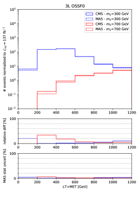
Figure 5.1: Comparison between CMS official distributions and the corresponding MadAnalysis 5 predictions. In the main panel, we present distributions for the trilepton signal regions dedicated to probing type-III seesaw models. The last bins contain the overflow. In the central insets, we show the bin-to-bin relative difference $\delta({\rm bin})$ in percent between the CMS and MadAnalysis 5 values, and in the lower insets, we indicate the statistical uncertainty $\delta_{MC}({\rm bin})$ in percent related to the Monte Carlo samples used for the MadAnalysis 5 predictions. The distributions in red and blue correspond respectively to scenarios with a $\Sigma$ mass set to 700 GeV and 300 GeV.

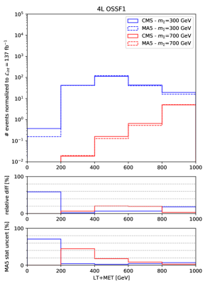
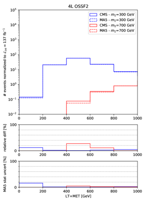
Figure 5.2: Same as in Figure 5.1 but for the four-lepton seesaw signal regions.

In the results shown in Figure 5.1 and Figure 5.2, we can see that the shapes of the distribution are generally quite well reproduced. For all signal regions but the 4L OSSF1 one, the relative difference is less than 20–30%. Such an order of magnitude is consistent with the theoretical and statistical uncertainties related to the signal, and the built-in differences in the analysis code and the detector simulation. For the signal region 4L OSSF1, a larger difference is observed for the first bin, but it also corresponds to a configuration in which the recast analysis lacks statistics. The indicator $\delta_{MC}$ indeed exhibits a high statistical uncertainty. The differences between CMS and MadAnalysis 5 are therefore considered as non-significant, an agreement being found in all the other bins, and we consider the implementation of the type-III seesaw signal regions as validated.

5.4 Validation of the implementation of the $t\bar{t}\phi$ signal regions

5.4.1 Event generation

To validate our implementation of the $t\bar{t}\phi$ signal regions, we consider a simple model implemented in FeynRules. It includes a new light $CP$-even scalar or $CP$-odd pseudoscalar boson, labeled $\phi$, which can is produced at the LHC through its Yukawa coupling $g_{t}$ to top quarks. The corresponding UFO model [100, 104] has been connected to MG_aMC@NLO in order to produce events at LO in QCD.

We produce the new boson $\phi$ in association with a top-antitop pair via its coupling $g_{t}$, and we assume that $\phi$ decays into a pair of charged leptons (electrons or muons) via a Yukawa coupling labeled $g_{l}$. The cross sections are calculated with the NNPDF3.0 LO set of PDF in the case where the product $g_{t}\cdot BR(\phi\rightarrow l^{+}l^{-})$ is equal to 0.05, and read $0.02160\pm 0.00216$ pb for a pseudoscalar boson with a mass of 20 GeV, and to $0.06597\pm 0.00660$ pb for a scalar boson with a mass of 70 GeV [101]. The associated theory errors are taken as reported by the CMS collaboration as no information is provided on how they have been evaluated. Concerning the (anti-)top quark, the decay into $Wb$ is forced with a branching ratio of 1, and the $W$ decay is handled by Pythia 8. Trilepton and four-lepton final state can arise from leptonic $W$-boson decays.

Pythia 8 is used in order to handle parton showering, hadronization, and the simulation of the underlying events (multiple interactions and beam remnant interactions). The underlying events tune is chosen to be CP5 [105].

A large statistics of events have been generated for each $\phi$ mass value and for each decay channel, as listed in Table 5.4.1.

List of produced signal samples for the validation of the $t\bar{t}\phi$ signal regions. $\phi$ scalar/pseudoscalar $\phi$ mass $\phi$ decay Number of produced events pseudoscalar 20 GeV $\phi\rightarrow\mu\mu$ 2,400,000 $\phi\rightarrow ee$ 4,400,000 scalar 70 GeV $\phi\rightarrow\mu\mu$ 2,400,000 $\phi\rightarrow ee$ 3,200,000

5.4.2 Comparison with CMS results

Public results provided by the CMS collaboration only consist of spectra of observables at the end of the selection. We therefore validate our implementation by comparing the distributions obtained with MadAnalysis 5 with the ones presented by CMS in Figures 5–10 of the analysis note. For low-mass $\phi$ (it is the case of our validation sample), the represented quantity is chosen to be the single attractor mass $M^{20}_{OSSF}$. The latter is defined as the invariant mass of the opposite-sign same-flavor lepton pair (OSSF) that is the closest to 20 GeV. Comparisons are performed in Figures 5.3, 5.4, 5.5, 5.6 and 5.7 for all $t\bar{t}\phi$ signal regions.

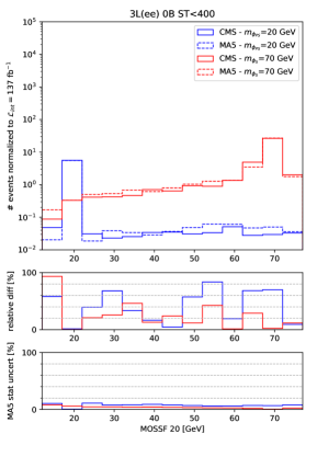
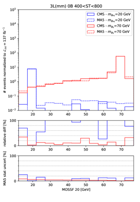
Figure 5.3: Same as in Figure 5.1 but for the first four trilepton signal regions dedicated to probing the $t\bar{t}\phi$ model. The distributions in red and blue correspond respectively to scenarios with a scalar of mass of 70 GeV, and a pseudoscalar of mass of 20 GeV.

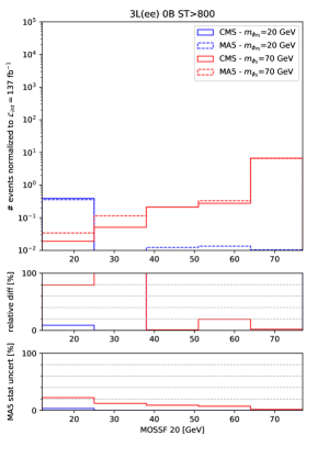
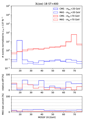
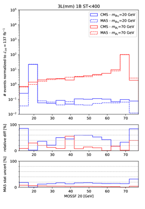
Figure 5.4: Same as in Figure 5.1 but for the next four trilepton signal regions dedicated to probing the $t\bar{t}\phi$ model. The distributions in red and blue correspond respectively to scenarios with a scalar of mass of 70 GeV, and a pseudoscalar of mass of 20 GeV.

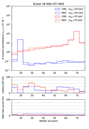
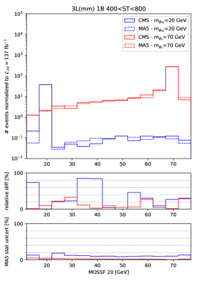
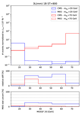
Figure 5.5: Same as in Figure 5.1 but for the last four trilepton signal regions dedicated to probing the $t\bar{t}\phi$ model. The distributions in red and blue correspond respectively to scenarios with a scalar of mass of 70 GeV, and a pseudoscalar of mass of 20 GeV.

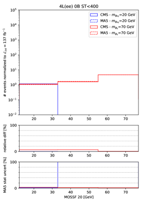
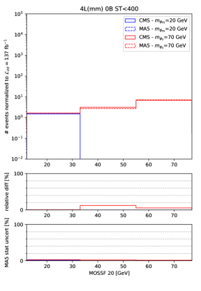
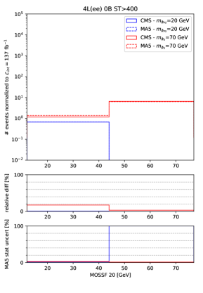
Figure 5.6: Same as in Figure 5.1 but for the first four four-lepton and no $b$-jet signal regions dedicated to probing the $t\bar{t}\phi$ model. The distributions in red and blue correspond respectively to scenarios with a scalar of mass of 70 GeV, and a pseudoscalar of mass of 20 GeV.

Figure 5.7: Same as in Figure 5.1 but for the last two four-lepton and no $b$-jet signal regions dedicated to probing the $t\bar{t}\phi$ model. The distributions in red and blue correspond respectively to scenarios with a scalar of mass of 70 GeV, and a pseudoscalar of mass of 20 GeV.

At first order, the recast analysis manages to reproduce quite well the distributions presented in the CMS paper. There are however noticeable differences. The two indicators $\delta({\rm bin})$ and $\delta_{MC}({\rm bin})$ defined in Section 5.3 are once again used for the interpretation of our findings and to quantify the level of agreement.

The statistics used for the validation of the recast analysis seems to be enough because the $\delta_{MC}({\rm bin})$ indicator is less than 10% for all signal regions. For signal regions in which the relative difference between the CMS and the recast predictions is large, we find first that the issue holds independently of the $\phi$ decay channel. The findings however allow us to interpret this difference as a consequence of a lack of statistics in the events used by the CMS collaboration (on which information is not provided). We can indeed observe that the CMS predictions are plagued with important statistical fluctuations, that are much larger than in the recast analysis. We therefore consider our implementation validated, at least at a level representative of what could be done with the information made public by the CMS collaboration.

5.5 Conclusions

We have presented the implementation of the multileptons search CMS-EXO-19-002 in the MadAnalysis 5 framework. This search considers proton-proton collisions at $\sqrt{s}=13~{}\textrm{TeV}$ and an integrated luminosity of 137 fb^-1. Samples of signal events relevant for both the type-III seesaw and $t\bar{t}\phi$ signal regions have been generated with MadGraph5_aMC@NLO at LO, then proccessed by Pythia 8 for parton showering, hadronization and mutiple parton interactions, and by Delphes 3 for the detector simulation. We have compared predictions made by MadAnalysis 5 with the official results provided by the CMS collaboration. The only public material for validation consist in key-observable distributions at the end of selection. We have considered various benchmark scenarios in both the electron and muon channel. The shapes of the distributions have been compared and are correctly reproduced for the seesaw signal regions. Discrepancies are found in the case of the $t\bar{t}\phi$ events, in particular in the trilepton channels. These can however be explained mainly by a lack of statistics of the CMS paper.

The MadAnalysis 5 C++ code is available, together with the material used for the validation of this implementation, from the MA5 dataverse (https://doi.org/10.14428/DVN/DTYUUE) [21].

Acknowledgments

We are very grateful to Yeonsu Ryou Juhee and Song and Kihong Park who have in the first place begun to work on this implementation. We are also indebted to Benjamin Fuks for his help and patience. We sincerely thank the organizers of the second MadAnalysis 5 workshop for their warm welcome in Seoul and the success of the event.

6 Implementation of the CMS-HIG-18-011 analysis (exotic Higgs decays via two pseudoscalars with two muons and two $b$-jets; 35.9 fb^-1)

By Joon-Bin Lee and Jehyun Lee

6.1 Introduction

In this note, we describe the validation of our implementation, in the MadAnalysis 5 framework [6, 7, 3, 8], of the CMS-HIG-18-011 search [22] for exotic decays of the Standard Model Higgs boson into a pair of light pseudoscalar particles $a_{1}$, where one of the pseudoscalar decays to a pair of opposite-sign muons and the other one decays into a pair of $b$-quarks. This analysis focuses on 13 TeV LHC data and an integrated luminosity of 35.9 $\rm fb^{-1}$.

The considered exotic decay of the Higgs boson is predicted in a variety of models, including the next-to-minimal supersymmetric extension of the Standard Model (NMSSM) [106], as well as models with additional scalar doublet and singlet (2HDM+S) [107, 108, 109]. To validate our implementation, we focus on an NMSSM setup in which one decouples most particles, except for the above-mentioned pseudoscalar states. Such a scenario has been studied in particular in the CMS-HIG-18-011 analysis that we implemented in this work.

In the rest of this note, we present a brief description of the CMS-HIG-18-011 analysis in section 6.2. Section 6.3 consists in the core of our work, and contains extensive information about the validation of our implementation. In particular, the presence of two $b$-jets in the final state makes this analysis particularly sensitive to the exact details of the $b$-jet identification algorithm. However, the $b$-jet identification efficiency provided by the CMS collaboration is not sufficient for a precise enough modeling in Delphes 3. The method that we used to model in an accurate manner the CMS $b$-tagging algorithm is therefore explained in details in Section 6.3.2. We summarise our work and results in section 6.4.

6.2 Description of the analysis

The CMS-HIG-18-011 analysis performs a search for the Higgs boson decay chain $h\rightarrow a_{1}a_{1}\rightarrow\mu^{+}\mu^{-}b\bar{b}$. This analysis hence targets a final state containing two opposite-sign muons and two $b$-tagged jets. In the next subsection, we present the definition of the muon and jet candidates that are used in this analysis, as well as the preselection cuts of the analysis. Then, in Section 6.2.2, we explain the event selection requirements leading to a good background rejection while preserving as many expected signal events as possible.

6.2.1 Object definitions and preselection

This analysis requires the presence of at least two final-state muons and two final-state $b$-jets. Two oppositely charged muons are required to conservatively satisfy an online selection based on the CMS muon triggering system. This enforces that the final state includes two muons with a transverse momentum $p_{T}>$ 17 GeV (leading muon $\mu_{1}$ ) and 8 GeV (subleading muon $\mu_{2}$). Moreover, the geometrical limitations of the CMS muon system leads to the following extra requirements on the muon’s $p_{T}$ and pseudorapidities $\eta$,

$$p_{T}({\mu_{1}})\ >\ 20\textrm{ GeV },\ p_{T}({\mu_{2}})\ >\ 9\textrm{ GeV }\ \text{and}\ \ |\eta({\mu_{1,2}})|\ <\ 2.4.$$ (6.1)

Additionally, a particle-flow-based relative isolation is enforced. This requires that the sum of the transverse energy of any detector-level object present in a cone of radius $R=0.4$ centered on the muon is smaller than 0.15 times the muon $p_{T}^{\mu}$,

$$I_{rel}=\frac{1}{p_{T}^{\mu}}\sum_{i}(p_{T})_{i}<0.15.$$ (6.2)

The CMS-HIG-18-011 analysis moreover targets a signal scenario in which the narrow width approximation is valid for the new pseudoscalar $a_{1}$, and its mass is considered to fulfil 20 GeV $\leq m_{a_{1}}\leq$ 62.5 GeV. The invariant mass of the two-muon system is, therefore, restricted to lie within a slightly wider mass range,

$$19.5\ \textrm{GeV}\ <m_{\mu\mu}\ <\ 63.5\ \textrm{GeV}.$$ (6.3)

Jets are reconstructed by clustering detector-level objects with the anti-$k_{T}$ algorithm [42] with a distance parameter of 0.4. The transverse momentum $p_{T}$ and pseudorapidity ($\eta$) of the leading jet $j_{1}$ and subleading jets $j_{i}$ (with $i\neq 1$) are imposed to satisfy

$$p_{T}({j_{1}})\ >\ 20\textrm{ GeV},\ p_{T}(j_{i})>15\textrm{ GeV and }|\eta(j_{1,i})|\ <\ 2.4.$$ (6.4)

Events must contain at least two jets, with the leading two jets having to be well separated from the selected muons in the transverse plane, by a distance $\Delta R>0.5$. $b$-tagging makes use of the CSVv2 algorithm [88] that relies on secondary vertex information. One of the jets must satisfy tight working point criteria, whereas another one has to satisfy loose working point requirements. The misidentification rate of light jets as $b$-jets is in average of 10% (0.1%) for the tight (loose) working point, and that of $c$-jets as $b$-jets is of 30% (2%), for a tagging efficiency of about 80% (40%). If there are more than two $b$-jets in the event, the two with the largest $p_{T}$ are considered as originating from a pseudoscalar $a_{1}$ decay.

Finally, the missing transverse momentum vector $\mathbf{p_{T}^{miss}}$ is defined as the opposite of the vector sum of the momentum of all reconstructed physics object candidates, and the missing transverse energy is defined by the norm of this vector,

$$E_{T}^{miss}=|\mathbf{p_{T}^{miss}}|.$$ (6.5)

6.2.2 Event Selection

Following the preselection described in the previous section, signal events are subjected to additional selection cuts to minimise the Standard Model background contamination. As the transverse momentum of the neutrinos arising from semi-leptonic $B$-hadron decays is small, we require,

$$E_{T}^{miss}\ <\ 60\ \textrm{GeV}.$$ (6.6)

Next, as both the muons and $b$-jets are the decay products of a pseudoscalar boson $a_{1}$, one requires that the values of the invariant mass of the dimuon system ($m_{\mu\mu}$) and that of the two-$b$-jet system ($m_{bb}$) are close to each other. Therefore, the relative difference between these two invariant masses is evaluated through a quantity $\chi_{bb}$ defined by

$$\chi_{bb}\ =\ \frac{(m_{bb}-m_{\mu\mu})}{\sigma_{bb}},$$ (6.7)

where $\sigma_{bb}$ is a mass resolution associated with the reconstruction of the two-$b$-jet system. The invariant mass of the whole system comprising those four objects ($m_{\mu\mu bb}$) should moreover be compatible with the Higgs-boson mass $m_{h}$. One subsequently defines the relative difference $\chi_{h}$,

$$\chi_{h}\ =\ \frac{(m_{\mu\mu bb}-m_{h})}{\sigma_{h}},$$ (6.8)

where $\sigma_{h}$ is the mass resolution associated with the reconstruction of the Higgs boson candidate ($\mu\mu bb$). Events are selected by requiring that the squared sum of these two variables, $\chi^{2}=\chi_{bb}^{2}+\chi_{h}^{2}$, is smaller than 5,

$$\chi^{2}\ <\ 5.$$ (6.9)

6.3 Validation

6.3.1 Event generation

In order to generate events necessary to valide our implementation, we use the NMSSMHET simplified model[109]. The latter involves two free parameters, the mass of pseudoscalar $m_{a_{1}}$ and tan$\beta$, that is defined as the ratio of the vacuum expectation values of the two Higgs doublets of the model. tan$\beta$ moreover determines the branching fraction of the $a_{1}$ boson to Standard Model particles. Following the CMS-HIG-18-011 analysis and the corresponding publicly available validation material, tan$\beta$ is set to 2 and we consider three pseudoscalar mass points,

$$m_{a_{1}}=20,\ 40,\ 60\ \textrm{GeV}.$$ (6.10)

As there is no strong dependence of the branching ratio $\mathcal{B}(a_{1}\rightarrow b\bar{b})$ and $\mathcal{B}(a_{1}\rightarrow\mu^{+}\mu^{-})$ on $m_{a_{1}}$ [109], the total signal cross section defined as the product of the Standard Model Higgs boson production cross section ($\sigma_{h}$) and the relevant branching fractions is set to a constant value,

$$\sigma_{h}\times\mathcal{B}(h\rightarrow a_{1}a_{1}\rightarrow\mu^{+}\mu^{-}b\bar{b})\approx 8\ \textrm{\rm fb}.$$ (6.11)

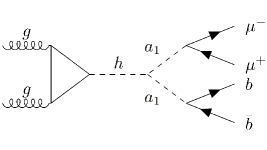
Figure 6.1: Feynman diagrams illustrating the two hard process considered in the event generation processes relevant for the validation of the implementation in the MadAnalysis 5 framework of the CMS-HIG-18-011 analysis. The signal comprises a gluon fusion component (left) and vector-boson fusion component (right).

We generate 1,000,000 events for each test sample. In order to mimic CMS signal event generation (so that we could compare our predictions to public material), we consider Higgs boson production via gluon fusion and vector boson fusion, as illustrated by the two Feynman diagrams shown in Figure 6.1. The total production cross sections resulting from a leading-order (LO) calculation achieved within the MadGraph5_aMC@NLO [46] framework and that are used for our signal normalisation, are, for each of the two subprocesses, 48.58 pb and 3.78 pb respectively.

The generation of the hard process is performed by using the NMSSMHET model implementation [109] in the UFO format [93], that can be used with the MadGraph5_aMC@NLO framework [46] at LO in QCD. Our matrix elements are convoluted with the NNPDF3.0 set of parton densities [95], and the Pythia 8.212 package [51] with the CUETP8M1 tune [102] is used to model parton showering and hadronisation.

The simulation of the response of the CMS detector is based on the Delphes 3 program [9], which internally relies on Fastjet [43] for object reconstruction. We start from the default CMS detector parametrisation and then impose modifications as follows.

First, the mimimum $p_{T}$ thresholds for muons and jets are reduced to 5 and 10 GeV respectively, in order to cover the full signal region.

Second, the muon and jet reconstruction efficiencies contained in the Run II CMS card in Delphes version 3.4.2 cannot cover such a small $p_{T}$ region. Therefore, they are extrapolated from the default ones to conservatively accept all objects used in this analysis.

Finally, the $b$-jet identification efficiencies based on the CSVv2 algorithm [88], which is used in CMS-HIG-18-011 analysis, have a large dependence on the jet transverse momentum. However, only average efficiency values are provided by the CMS collaboration. To approximatively model the $p_{T}$ dependence of the combined secondary vertex algorithm used in this work, we have used the efficiency functions associated with the loose working point of the deep combined secondary vertex (DeepCSV) algorithm described in the CMS $b$-jet identification paper [88]. These are then re-weighted via the average tagging efficiencies of the CSVv2 algorithm, as further described in the next section. This re-weighting method has the great advantage of reflecting not only the overall $b$-tagging power of the CSVv2 algorithm, but also the $p_{T}$ dependence of this general CMS $b$-tagging algorithm.

6.3.2 Refinements of our event selection

This work uses the same event selection as described in Section 6.2. However, additional details are necessary to reproduce the CMS-HIG-18-011 results. This section first describes the re-weighting method that we used to improve the modeling of the $b$-tagging performance in Delphes 3, and then explains how to estimate the mass resolutions $\sigma_{bb}$ and $\sigma_{h}$ that are needed to calculate the $\chi_{bb}$ and $\chi_{h}$ quantities of Section 6.2.

As noted in Section 6.3.1, the HIG-18-011 analysis used the CSVv2 $b$-tagging algorithm. The average efficiencies and mistagging rates of this algorithm are provided in the CMS $b$-jet identification publication [88], but there is no information about their $p_{T}$ dependence. We have however found out that ignoring this $p_{T}$ dependence can make a difference of about 20 % in the final results.

To recover this, we assume that the $p_{T}$ dependence of the DeepCSV and CSVv2 algorithms is similar. This assumption is justified as both methods use an almost identical approach based on combined information originating from displaced tracks and secondary vertices. We hence implement the publicly available loose $b$-tagging efficiency and mis-tagging rates of the DeepCSV algorithm in Delphes 3, with their full dependence on the jet’s transverse momentum. In a second step, we re-weight the generated events to account for the different average efficiencies associated with the loose working points of the DeepCSV and CSVv2 algorithms. In practice, we use as a re-weghting factor the squared ratio of the $p_{T}$-independent efficiencies, $(\bar{\epsilon}^{v2}_{L}/\bar{\epsilon}^{D}_{L})^{2}$, where $\bar{\epsilon}^{v2}_{L}$ and $\bar{\epsilon}^{D}_{L}$ are respectively the CSVv2 and DeepCSV algorithm efficiencies as provided in the CMS $b$-tagging performance publication [88].

At last, the signal region event selection requires that at least one jet passes the requirement of the tight $b$-jet discriminator. The final event weight is therefore calculated as

$$w=\Bigg{(}\frac{\bar{\epsilon}^{v2}_{L}}{\bar{\epsilon}^{D}_{L}}\Bigg{)}^{2}\cdot\Bigg{[}1-\bigg{(}1-\frac{\epsilon^{v2}_{T}(j_{i})}{\epsilon^{v2}_{L}(j_{i})}\bigg{)}\cdot\bigg{(}1-\frac{\epsilon^{v2}_{T}(j_{j})}{\epsilon^{v2}_{L}(j_{j})}\bigg{)}\Bigg{]}.$$ (6.12)

In this equation, $\epsilon^{v2}_{T(L)}(j_{i})$ represents the efficiency that the $i^{\rm th}$ jet ($j_{i}$) satisfies the tight (loose) CSVv2 selection criteria, that we estimate again from DeepCSV public information,

$$\epsilon^{v2}_{T,L}(j_{i})=\frac{\bar{\epsilon}^{v2}_{T,L}}{\bar{\epsilon}^{D}_{T,L}}\cdot\epsilon^{D}_{T,L}(j_{i}).$$ (6.13)

Here, $\epsilon^{D}_{T,L}(j_{i})$ are the DeepCSV tight and loose $p_{T}$-dependent efficiencies.

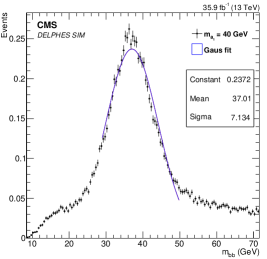
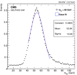
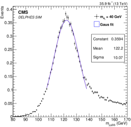
Figure 6.2: The di-$b$-jet invariant-mass distribution with its Gaussian fitting, for pseudoscalar mass scenarios of $m_{a_{1}}$ = 20 (left), 40 (center), and 60 (right) GeV.

Figure 6.3: The invariant-mass distribution of the reconstructed Higgs boson candidate, with its Gaussian fitting for pseudoscalar mass scenarios of $m_{a_{1}}$ = 20 (left), 40 (center), and 60 (right) GeV.

After the signal region selection of two jets and two muons, the mass resolutions of the di-$b$-jet ($\sigma_{bb}$) and reconstructed Higgs boson candidate ($\sigma_{h}$) are estimated by fitting the corresponding invariant-mass distributions with Gaussian functions. However, the CMS analysis note does not provide the exact values of these resolutions as obtained from the fit. We have therefore estimated these values by performing our own fit of the invariant-mass distributions.

As a rough approximation, we estimate the input values of the mass resolutions $\sigma_{bb}^{i}$ and $\sigma_{h}^{i}$ that are used in our Gaussian fitting procedure from the muon and jet $p_{T}$ resolutions of the CMS detector. Each muon and jet originating from the Higgs boson decay has an average transverse momentum of about 30 GeV. The momentum resolution of a 30 GeV muon is expected to be of about 1% [110], whereas that of a 30 GeV jet is expected to be of about 17% [111]. Based on these values, the initial input mass resolution of the di-$b$-jet system is set to $\sigma_{bb}^{i}=0.17m_{a_{1}}$, and the one of the reconstructed Higgs boson candidate is fixed to $\sigma_{h}^{i}=9.3$ GeV. Our Gaussian fitting is then performed within a fitting range of $m_{a_{1}(h)}\pm 1.5\sigma_{bb(h)}^{i}$ from the above input values.

Figure 6.3 and 6.3 show the invariant-mass distributions of the di-$b$-jet system and of the reconstructed Higgs boson candidate, together with the corresponding Gaussian fit results. The average mass resolution of the di-$b$-jet system is found to be $0.173m_{a_{1}}$, whilst that of the Higgs boson candidate is equal to 9.66 GeV. As a result, the $\chi_{bb}$, $\chi_{h}$ and $\chi^{2}=\chi_{bb}^{2}+\chi_{h}^{2}$ quantities can be calculated by using eqs. (6.7) and (6.8).

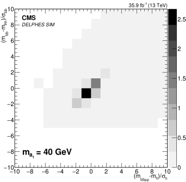
Figure 6.4: Left: The $\chi^{2}$ distribution associated with the scenario in which $m_{a_{1}}$ = 40 GeV, once all analysis selections except the $\chi^{2}<5$ requirement are applied. Right: Two-dimensional distribution of the $(m_{bb}-m_{\mu\mu})/\sigma_{bb}$ and $(m_{\mu\mu bb}-125~{}{\rm GeV})/\sigma_{h}$ quantities for the same scenario and after applying all the cuts of the analysis with the exception of the $\chi^{2}<$ 5 requirement.

In the left panel of Figure 6.4, we show the $\chi^{2}$ distribution that is obtained after applying all selections except the $\chi^{2}<5$ cut. The results are presented for a scenario in which the mass of the pseudoscalar $a_{1}$ is fixed to 40 GeV. In the right panel of the figure, we moreover show the two-dimensional distribution of the $\chi_{bb}$ and $\chi_{h}$ quantities for the same scenario and after applying again all analysis cuts but the last one. This illustrates the quality of our fit and its impact on the signal reconstruction.

6.3.3 Comparison with official results

To validate our results, we compare predictions obtained with our MadAnalysis 5 implementation (and our tuned detector simulation based on Delphes 3) to the CMS official results presented in the CMS-HIG-18-011 analysis note for the three considered new physics scenarios. As a first test, we compare the curve shown in the left panel of Figure 6.4 to the first figure (Fig. 1) of the CMS note. The shape of the two distributions are similar, the values in the most populated first bins being found to differ by at most a few percent. We additionally compare the shape of the contours shown in the right panel of Figure 6.4 with the one exhibited in the second figure (Fig. 2) of the CMS publication. Here, the central bin are even populated equally. As already mentioned in the previous section, this validates our fitting procedure.

Event yields resulting from the object selection of Section 6.2.1 (the so-called $\mu^{+}\mu^{-}b\bar{b}$ selection) and after the final selection cuts presented in Section 6.2.2. The results are normalised to an integrated luminosity of 35.9 $\rm fb^{-1}$. We moreover include the total event selection efficiencies ($\epsilon$) for three mass scenarios. We compare predictions obtained with MadAnalysis 5 and the public CMS results. $\mu^{+}\mu^{-}b\bar{b}$ selection Final selection $\epsilon$ (%) $m_{a_{1}}$ = 20 GeV CMS-HIG-18-011 $14.0\pm 0.1$      $6.0\pm 0.1$ $42.9$ MA5 Recasting $13.2$      $5.6$ $42.5$ Difference $\delta$ (%) $5.7$      $6.7$ $0.4$ $m_{a_{1}}$ = 40 GeV CMS-HIG-18-011 $14.8\pm 0.1$      $7.5\pm 0.1$ $50.7$ MA5 Recasting $15.9$      $7.4$ $46.2$ Difference $\delta$ (%) $7.4$      $1.3$ $4.5$ $m_{a_{1}}$ = 60 GeV CMS-HIG-18-011 $16.7\pm 0.1$      $10.1\pm 0.1$ $60.5$ MA5 Recasting $16.9$      $10.1$ $60.0$ Difference $\delta$ (%) $1.2$      $0.3$ $0.5$

In Table 6.3.3, we compare CMS public yields with the recasting results predicted with MadAnalysis 5 after the object definition selection of Section 6.2.1, i.e. before applying the $p_{T}^{miss}<$ 60 GeV and $\chi^{2}<$ 5 requirements, and after the full analysis selection. The differences between the CMS and MadAnalysis 5 event yields ($N^{\rm CMS}$ and $N^{\rm MA5}$) is quantified through relative differences,

$$\delta=\frac{|N^{\rm CMS}-N^{\rm MA5}|}{N^{\rm CMS}}$$ (6.14)

Overall results agree at the level of the few percent, where the best agreement is achieved for the final selection with the 60 GeV pseudoscalar mass scenario which only shows a 0.3 % difference with the CMS-HIG-18-011 results from Ref. Sirunyan:2018mot. Event selection efficiencies ($\epsilon$) and the corresponding differences are also computed. The level of agreement between the CMS results and the MadAnalysis 5predictions is again found to lie at the percent level.

Although the event yields exhibit a larger difference after the object definition selection (ranging up to 7.4% for the $m_{a_{1}}=40$ GeV scenario), we consider that such a feature should be expected as resulting from our approximate modeling of the $p_{T}$ dependence of the $b$-tagging performance. Such an order of magnitude is indeed typical from the differences originating from the use of the DeepCSV and CSVv2 algorithms. We nevertheless consider this as a minor effect stemming from the lack of public knowledge about the new $b$-tagging algorithms used by CMS.

Even after adding the impact of our method to estimate the mass resolutions used in the CMS-HIG-18-011 analysis, only a small difference between MadAnalysis 5 predictions and CMS official results remains. We take it as sufficiently acceptable to guarantee the validation of our recast. Unfortunately, our validation cannot be performed further because of the lack of available public information.

6.4 Conclusion

In this note, we have documented a recast in the MadAnalysis 5 frsmework of the CMS-HG-18-011 search for light pseudoscalar particles originating from an exotic decay of the Standard Model Higgs boson. This search considers a final state comprising two $b$-jets and a pair of opposite-sign muons, and an integrated luminosity of 35.9 $\rm fb^{-1}$ of data collected at a centre-of-mass energy of 13 TeV.

Our work features two important differences with respect to what CMS has done. First, due to the lack of public knowledge about the transverse momentum dependence on the CSVv2 $b$-tagging algorithm performances, we have modeled our $b$-tagging efficiencies and mistagging rates in Delphes 3 by using the dependence of the DeepCSV algorithm performances on the transverse momentum of the jets. We have moreover included an event re-weighting procedure dealing with the differences between the average tagging efficiencies of the two algorithms. Second, we had to implement our own Gaussian fitting procedure to recover the invariant-mass resolutions expected from the signal, in the case of the reconstructed Higgs boson and pseudoscalar boson $a_{1}$. These are extensively detailed in Section 6.3.2.

To validate our implementation of the above search, we generated three signal samples in accordance with the CMS prescriptions. We have found that our approximate treatment of the mass resolutions and the CMS $b$-tagging performance are reasonable enough. These has allowed us to obtained an agreement with the CMS results at the level of a few percent. In contrast, only a poor level of agreement of about 20% can be reached without implementing our two classes of changes.

Subsequently to the lack of public CMS information for this analysis, we have only validated our code by comparing a few differential distributions and event yields at two stages of the full event selection. Our results exhibit a reliable agreement at the percent level. The implemented code is available online from the MadAnalysis 5 dataverse [23], at https://doi.org/10.14428/DVN/UOH6BF, which also includes the cards and UFO model that have been used in our validation procedure.

7 Implementation of the ATLAS-SUSY-2018-04 analysis (stau pairs with two taus and missing transverse energy; 139 fb^-1)

By Jongwon Lim, Chih-Ting Lu, Jae-Hyeon Park and Jiwon Park

7.1 Introduction

In this note, we describe the validation of the implementation, in the MadAnalysis 5 framework [8, 3, 7, 6], of the ATLAS-SUSY-2018-04 search [24] for direct stau production in events featuring two hadronic tau leptons and a large amount of missing transverse energy ($E^{miss}_{T}$). This analysis focuses on LHC proton-proton collisions at a center-of-mass energy of 13 TeV, and considers an integrated luminosity of $139{\rm fb}^{-1}$. The typical supersymmetric signal which this analysis is dedicated to is illustrated by the representative Feynman diagram shown in Fig. 7.1.

For the validation of our re-implementation, we have focused on a simplified model in which only a few electroweakly-interacting superpartners are relevant. The lightest neutralino ($\tilde{\chi}^{0}_{1}$) is taken as the lightest supersymmetric particle (LSP). The stau-left ($\tilde{\tau}_{L}$) and stau-right ($\tilde{\tau}_{R}$) sleptons are moreover assumed to be mass degenerate and they do not mix. Therefore the gauge eigenstates ($\tilde{\tau}_{L}$,$\tilde{\tau}_{R}$) coincide with the mass eigenstates ($\tilde{\tau}_{1}$,$\tilde{\tau}_{2}$) in this theoretical framework. Furthermore, in order to suppress any other decay modes of the tau sleptons, the masses of all charginos and neutralinos are set to 2.5 TeV except for the $\tilde{\chi}^{0}_{1}$ neutralino. Hence, the single kinematically allowed decay mode of the staus is

$$\tilde{\tau}\rightarrow\tilde{\chi}^{0}_{1}\tau$$ (7.1)

Finally, all squarks, that do not contribute at leading-order, are decoupled as well.

This note is organized as follows. In Sec. 7.2, we present an outline of the analysis under consideration. It in particular includes definitions for the physics objects and event selections that we have implemented for our recasting exercise. Sec. 7.3 is dedicated to event generation in the context of the two considered benchmark for the validation or our re-implementation, and includes a comparison with official ATLAS results. In Sec. LABEL:sec:conc, we summarize our work.

7.2 Description of the analysis

This analysis targets a final state containing two hadronic tau leptons with a certain amount of missing transverse energy. The kinematics of the di-$\tau+E^{miss}_{T}$ system is used to reduce the contributions from Standard Model backgrounds. In Sec. 7.2.1, we first detail how the objects relevant for the analysis are reconstructed and defined. Then, in Sec. 7.2.2, we discuss the sequence of event selections that are applied in the aim of unravelling the signal from the background.

7.2.1 Object definitions

Jets are reconstructed by means of the anti-$k_{t}$ algorithm [42] with a radius parameter set to $R=0.4$. This analysis focuses on jets whose transverse momentum $p^{j}_{T}$ and pseudorapidity $\eta^{j}$ fulfill

$$p^{j}_{T}>20\textrm{ GeV}\quad\textrm{and}\quad|\eta^{j}|<2.8.$$ (7.2)

Moreover, the selected jets that are tagged as originating from the fragmentation of a $b$-quark must satisfy the stronger requirements

$$p^{b}_{T}>20\textrm{ GeV}\quad\textrm{and}\quad|\eta^{b}|<2.5.$$ (7.3)

In the considered analysis, a $b$-tagging working point with an average efficiency of $77\%$ is used. This working point corresponds to $c$-jet and light-jet rejection rates of $4.9$ and $110$, respectively.

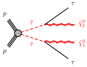
Figure 7.1: The Feynman diagram for the process $pp\rightarrow\tilde{\tau}\tilde{\tau}\rightarrow\tilde{\chi}^{0}_{1}\tilde{\chi}^{0}_{1}\tau\tau$.

Electron candidates are required to have a transverse momentum $p^{e}_{T}$ and pseudorapidity $\eta^{e}$ obeying

$$p^{e}_{T}>17\textrm{ GeV}\quad\textrm{and}\quad|\eta^{e}|<2.47.$$ (7.4)

Furthermore, all electron candidates are required to have both track and calorimeter isolations. The condition of the track isolation is

$$\sum p_{T,\textrm{tracks}}/p^{e}_{T}<0.15\quad\textrm{with}\quad\Delta R=\min(10\textrm{ GeV}/p^{e}_{T},0.2),$$ (7.5)

the condition of the calorimeter isolation is

$$\sum E_{T,\textrm{calorimeter}}/p^{e}_{T}<0.2\quad\textrm{with}\quad\Delta R=0.2,$$ (7.6)

and for high transverse momentum electron, we use instead of the two above conditions

$$\sum E_{T,\textrm{calorimeter}}<\max(0.015\times p^{e}_{T},3.5\textrm{ GeV})\ \ \textrm{with}\ \ \Delta R=0.2\ \ \textrm{if}\ \ p^{e}_{T}>200\textrm{ GeV}.$$ (7.7)

Muon candidate definition is similar, although with slightly looser thresholds,

$$p^{\mu}_{T}>14\textrm{ GeV}\quad\textrm{and}\quad|\eta^{\mu}|<2.7,$$ (7.8)

The condition of the track isolation is

$$\sum p_{T,\textrm{tracks}}/p^{\mu}_{T}<0.15\quad\textrm{with}\quad\Delta R=\min(10\textrm{ GeV}/p^{\mu}_{T},0.3),$$ (7.9)

and the condition of the calorimeter isolation is

$$\sum E_{T,\textrm{tracks}}/p^{\mu}_{T}<0.3\quad\textrm{with}\quad\Delta R=0.2.$$ (7.10)

In the ATLAS experiment, hadronically decaying tau lepton ($\tau_{had}$) candidates are reconstructed with one or three associated charged pion tracks (prongs). For 1-prong (3-prong) $\tau$ lepton candidates, the signal efficiencies are $75\%$ and $60\%$ for the medium working point respectively. In the recasting based on MadAnalysis 5 that we implement in this work, the simulation of the detector response is performed with the Delphes 3 [9] software. We consider a tau-tagging efficiency of $100\%$ with a misidentification probability of $0\%$ at the level of Delphes 3, and handle medium and tight tau-tagging efficiencies through event reweighting factors extracted from the official ATLAS cutflow tables. Those factors are evaluated and included at the level of the analysis. Further details are given in Sec. 7.2.2.

Baseline tau lepton candidates are required to have

$$p^{\tau}_{T}>50\ (40)\textrm{ GeV}\quad\textrm{and}\quad|\eta^{\tau}|<2.5$$ (7.11)

for the leading (subleading) candidates, and the transition region between the barrel and endcap calorimeters ($1.37<|\eta^{\tau}|<1.52$) is excluded.

The object definition ends with some overlap removal conditions. The latter are implemented consistently to the analysis code provided through HEPData[112]. Tau leptons are removed if they are too close to an electron or a muon, with $\Delta R(\tau,e/\mu)<0.2$. Electrons are then removed if they are too close to a muon, with $\Delta R(e,\mu)<0.01$. Next, the jet collection is cleaned from those jets lying at an angular distance $\Delta R(j,e/\mu)<0.2$ of a muon or an electron, and the electrons and muons that are too close to any of the remaining jets are removed if $\Delta R(e/\mu,j)<0.4$. Finally, jets are removed if they are too close to one of the tau lepton candidates, with $\Delta R(j,\tau)<0.2$.

7.2.2 Event selection

Because Delphes 3 utilizes simplified and parameterized approaches to simulate different elements of the detector response, it is hard to emulate some of the properties relevant for the ATLAS-SUSY-2018-04 analysis, and therefore implement certain cut steps precisely. As a consequence, we have modelled several selections through event reweighting. This concerns first the trigger efficiency. Next, several reweighting factors are included to model specific features of the tau-tagging-based selections. This allows us to define the so-called medium and tight tau lepton cuts in our implementation, from an ideal detector parameterization in Delphes 3.

After the object definitions introduced in the previous subsection, events with exactly two baseline tau leptons are selected. All events are required to pass either an asymmetric di-$\tau$ trigger for the low stau mass region (SR-lowMass) or a combined di-$\tau+E^{miss}_{T}$ ($E^{miss}_{T}>150$ GeV) trigger for the high stau mass region (SR-highMass). This is coined trigger and offline cuts below. A trigger efficiency of $80\%$ is applied in our recasting, after that we impose that the transverse momenta of the two leading tau candidates are larger than the offline $p_{T}$ thresholds given in Table 7.2.2. In order to deal with the different tau candidate kinematic cuts that are applied in the 2015–2017 and 2018 data-taking periods, we randomly tag each event as originating from the 2015–2017 or 2018 data set. In practice, the probability of imposing the 2015–2017 (2018) data set thresholds is calculated from the ratio of the 2015–2017 (2018) integrated luminosity to the total luminosity of $139~{}{\rm fb}^{-1}$.

Moreover, we assume that the tau leptons which fired the triggers are those selected through the offline cuts. A trigger-level $\tau_{had}$ identification efficiency of 0.9 is correspondingly applied for each reconstructed tau lepton, which mimics the medium tau identification procedure for a tau lepton passing both online and offline requirements [113]. This leads to a total trigger reweighting factor of 64.8% that includes a global trigger efficiency of 80% and individual tau reconstruction efficiencies of 90%.

Offline $p_{T}$ thresholds for the leading (subleading) tau lepton candidate, in the case of the asymmetric di-$\tau$ (second column) and di-$\tau+E^{miss}_{T}$ (third column) triggers. This corresponds to a ditau efficiencies of about $80\%$. Year asymmetric di-$\tau$ di-$\tau+E^{miss}_{T}$ 2015-2017 95 (60) GeV 50 (40) GeV 2018 95 (75) GeV 75 (40) GeV

After the handling of the triggers described above, events with exactly two medium tau lepton candidates with opposite-sign (OS) electric charges are selected. To treat the efficiency of selecting two offline mediumly tagged OS taus on top of a di-tau(+$E^{miss}_{T}$) trigger selection (as Delphes does not simulate charge misidentification), an additional event reweighting factor of 0.7 is enforced. This number is evaluated from the average ratio of the cut efficiencies provided by the ATLAS collaboration and those predicted by MadAnalysis 5 when the identification of two medium taus is not included at the cutflow step called 2 medium $\tau$ (OS) and 3rd medium $\tau$ veto below.

In the next selection steps, a $b$-jet veto is enforced to reject events originating from top quark processes. Also, events featuring any additional light leptons (muons or electrons) are rejected. Finally, selection cuts common to both signal regions also include constraints on the reconstructed invariant mass of the two leading tau lepton system, $m(\tau_{1},\tau_{2})$. The latter is required to be larger than $120$ GeV, in order to remove events exhibiting a pair of tau leptons stemming from low-mass resonances, $Z$ boson, and Higgs boson decays ($Z/H$ veto).

In the SR-lowMass region, a missing energy constraint of 75 GeV $<E^{miss}_{T}<150$ GeV is imposed to increase the signal sensitivity. Moreover, the two selected tau leptons are required to be tight tagged. The selection efficiency $p_{tight}$ associated with two medium taus passing the tight working point requirements is extracted from the official ATLAS cutflow tables. We rely on the ratio of the number of surviving weighted events before applying the tight tau lepton requirement, and after applying it. We use $p_{tight}\simeq 0.70$.

In the SR-highMass region, the tight tagging efficiency is extracted similarly, with the exception that at least one of two tau leptons should pass the tight selection requirements and not both of them). We use here $p_{tight}+2\sqrt{p_{tight}}(1-\sqrt{p_{tight}})\simeq 0.91$.

The stransverse mass $m_{T2}$ variable [114, 115] is defined as

$$m_{T2}=min_{\mathbf{q}_{T}}\left[max(m_{T,\tau_{1}}(\mathbf{p}_{T,\tau_{1}},\mathbf{q}_{T}),m_{T,\tau_{2}}(\mathbf{p}_{T,\tau_{2}},\mathbf{p}^{miss}_{T}-\mathbf{q}_{T}))\right],$$ (7.12)

where $\mathbf{p}_{T,\tau_{1}}$ and $\mathbf{p}_{T,\tau_{2}}$ are the transverse momenta of the two tau lepton candidates. The transverse momentum vector of one of the invisible particle, $\mathbf{q}_{T}$, is chosen to minimize the larger of the two transverse mass $m_{T,\tau_{1}}$ and $m_{T,\tau_{2}}$. The transverse mass $m_{T}$ is defined by

$$m_{T}(\mathbf{p}_{T},\mathbf{q}_{T})=\sqrt{2(p_{T}q_{T}-\mathbf{p}_{T}\cdot\mathbf{q}_{T})}.$$ (7.13)

In MadAnalysis 5, the $m_{T2}$ calculation can be done automatically through the function PHYSICS->Transverse->MT2(vec1,vec2,ETmiss,Minvisible). In this expression, vec1 and vec2 stand for the two visible momenta, ETmiss for the miissing transverse momentum and Minvisible for a test mass that should map the expected mass of the invisible state.

A lower bound on the $m_{T2}$ variable of 70 GeV is imposed, in order to reduce the contamination from $t\overline{t}$ and $WW$ events. Finally, the two tau lepton candidates are required to be well separated in the transverse plane, by $\Delta R(\tau_{1},\tau_{2})<3.2$ and $|\Delta\phi(\tau_{1},\tau_{2})|>0.8$ to further suppress the contributions of the Standard Model backgrounds.

7.3 Validation

Cut-flow associated with a simplified model benchmark scenario defined by $m(\tilde{\tau},\tilde{\chi}^{0}_{1})=(120,1)$ GeV and for the $pp\to\tilde{\tau}\tilde{\tau}$ production process. We compare ATLAS official results and MadAnalysis 5 predictions through the expected number of events after each cut and the corresponding efficiencies, and indicate their difference $\delta$.

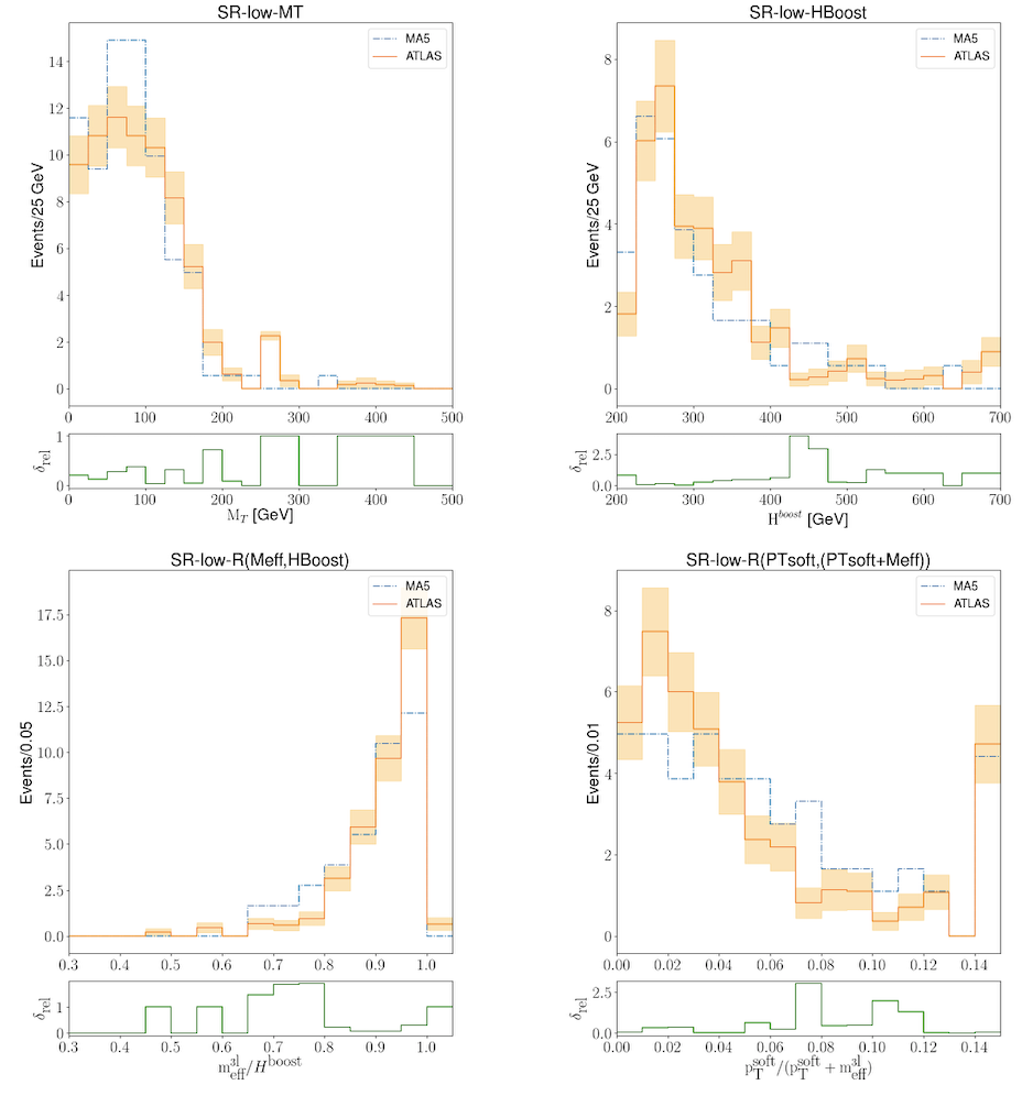
Figure 8.2: Comparison of several differential distributions as predicted by MadAnalysis 5 with the official results provided by the ATLAS collaboration, for the SR-LOW region. The official results provided by the ATLAS collaboration are shown with their uncertainties. The SR-LOW event selections are applied for each distribution except for the variable shown.

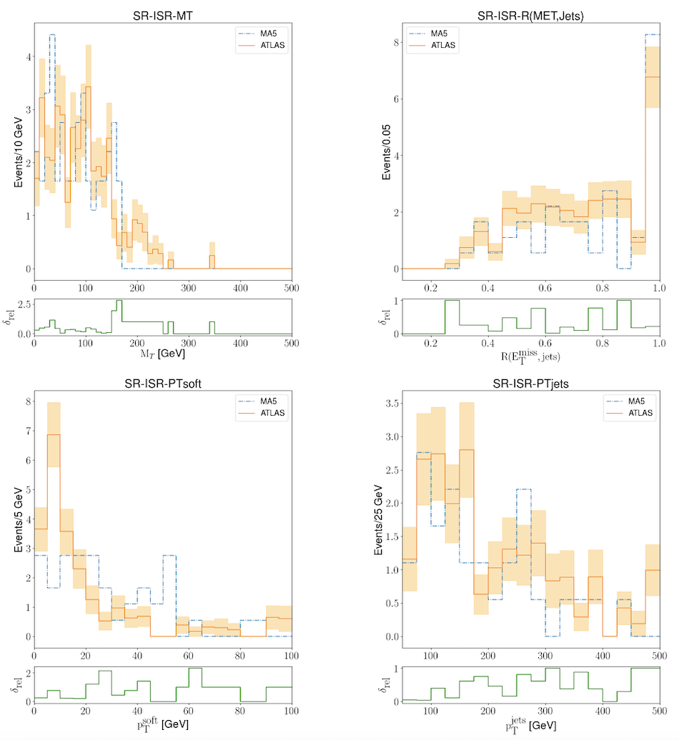
Figure 8.3: Comparison of several differential distributions as predicted by MadAnalysis 5 with the official results provided by the ATLAS collaboration, for the SR-ISR region. The official results provided by the ATLAS collaboration are shown with their uncertainties. The SR-ISR event selections are applied for each distribution except for the variable shown.

8.4 Conclusions

The MadAnalysis 5 implementation of the ATLAS-SUSY-2018-06 analysis, a search for the production of electroweakinos with the three-lepton final state has been presented. The ATLAS collaboration found excesses of three-lepton events in two signal regions, the low-mass region SR-LOW, and the initial-state radiation region SR-ISR. Validation was done by comparing the efficiency of various selection cuts that has been provided by the ATLAS collaboration with the result predicted by the MA5 framework. We found that the difference between the two was quite acceptable with differences at the level of at most 20%. Thus, we concluded that the analysis reimplementation is validated. The material that has been used for the validation of this implementation is available, together with the MadAnalysis 5 C++ code, at the MA5 dataverse (https://doi.org/10.14428/DVN/LYQMUJ) [27].

Acknowledgments

We thank all the chairpersons for their help. Particularly, special thanks to Benjamin Fuks, Jack Araz for fruitful discussion, as well as Eric Conte, Dipan Sengupta, and Si Hyun Jeon for their help.

9 Implementation of the ATLAS-SUSY-2018-31 analysis (sbottoms with multi-bottoms and missing transverse energy; 139 fb^-1)

By Jack Y. Araz and Benjamin Fuks

9.1 Introduction

The popularity of supersymmetry (SUSY) mostly arises as it provides, by extending the Poincaré algebra and by linking the fermionic and bosonic content of the theory, an elegant solution to the hierarchy problem inherent to the Standard Model (SM). In the Minimal Supersymmetric Standard Model (MSSM) [123, 124], each of the SM degree of freedom is associated with a supersymmetric partner. After the breaking of the electroweak symmetry, the partners of the gauge and Higgs fields mix into four neutralino ($\tilde{\chi}^{0}_{1,2,3,4}$) and two chargino ($\tilde{\chi}^{\pm}_{1,2}$) mass eigenstates, the lightest neutralino being often taken as a viable candidate for dark matter. In order for the MSSM to consist of a solution for the hierarchy problem, the supersymmetric partners of the top and bottom quarks are in general required to be quite light, so that their quadratic contributions to the quantum corrections to the Higgs boson mass stay under control [130, 131]. They have thus the possibility to be copiously pair-produced at the LHC.

The ATLAS-SUSY-2018-31 analysis [28] has been designed to investigate the possibility of such light sbottoms, and probes multi-bottom final states additionally featuring a large amount of missing transverse energy. The signature under consideration could arise from sbottom pair production followed by $\tilde{b}\to\tilde{\chi}^{0}_{2}b$ decays, where the second neutralino further decays into an SM Higgs boson and a lightest neutralino,

$$pp\to\tilde{b}\tilde{b}^{*}\to(\tilde{\chi}^{0}_{2}b)(\tilde{\chi}^{0}_{2}\bar{b})\to(\tilde{\chi}^{0}_{1}hb)(\tilde{\chi}^{0}_{1}h\bar{b})\ .$$ (9.1)

A representative Feynman diagram for the above process is shown in figure 9.1. Such a decay pattern is predicted to be enhanced in MSSM scenarios in which the lightest state $\tilde{\chi}^{0}_{1}$ is bino-like and the heavier state $\tilde{\chi}^{0}_{2}$ is wino-like, the $\tilde{b}\to\tilde{\chi}^{0}_{1}b$ and $\tilde{b}\to\tilde{\chi}^{-}_{1}t$ decays being in this case suppressed. The kinematics of the final-state objects largely depend on the mass spectrum of the various involved particles. Whilst a rather split spectrum gives rise to high-$p_{T}$ $b$-jets, a compressed spectrum leads, on the other hand, to relatively soft $b$-jets.

The ATLAS-SUSY-2018-31 analysis has been divided into three main signal regions SRA, SRB and SRC. Region SRA is dedicated to final states including at least four hard $b$-jets arising both from Higgs-boson and sbottom decays. Region SRB aims to track relatively softer $b$-jets which are originating from sbottom decays, together with a harder leading jet dawned from initial-state radiation. Finally, region SRC targets a topology with softer $b$-jets that are all well separated from the missing energy, which gives rise to a sizeable missing energy significance. This analysis has been found to constrain sbottom masses ranging up to 1.5 TeV in the corresponding simplified models.

In the rest of this note, we present the recast of the ATLAS-SUSY-2018-31 analysis of Ref. [28] in the MadAnalysis 5/SFS framework [10] that relies on smearing and efficiency functions for the simulation of the detector response. The code of our implementation is available from the MadAnalysis 5 dataverse [29], and the Monte Carlo cards relevant for the validation have been obtained from HEPData[132].

9.2 Description of the analysis

The considered analysis focuses on a signature made of multiple $b$-jets and missing transverse energy, which could originate from sbottom pair-production and cascade decays. As mentioned above, the results are interpreted in three classes of simplified models, two of which being relevant for compressed mass spectra and the third one being representative of split spectra. The topology in question is illustrated by figure 9.1 and by eq. (9.1).

9.2.1 Object definitions

Jets are obtained by clustering all final-state objects of a given event, with the exception of muons (and invisible particles as the latter are present in typical Monte Carlo event records). Electrons and photons being included, an overlap removal procedure is in order. This is detailed below. Jet clustering relies on the anti-$k_{T}$ algorithm with a radius parameter set to $R=0.4$ [42], that is used within the FastJet package version 3.3.3 [43].

Two types of jets are considered in this analysis. First, baseline jets are enforced to have a transverse momentum $p_{T}>20$ GeV, and a pseudorapidity satisfying $|\eta|<4.8$. Signal jets are obtained from this collection, after the object removal procedure described below.

Figure 9.1: Representative Feynman diagram for sbottom pair production, followed by sbottom cascade decays through the second neutralino. The figure has been retrieved from ref. [28].

Hadronic taus are extracted from the full jet collection, analysis-level tau candidates having a transverse momentum $p_{T}>2.5$ GeV and a pseudorapidity fulfiling $|\eta|<2.5$. The tau-tagging performance are taken from ref. [113], the tagging efficiency being in average of 60% for a mistagging rate of light jets as hadronic taus of 1%.

The initial sets of leptons are those electrons and muons that are reconstructed from final-state objects after imposing loose electron identification requirements [40], and medium muon identification requirements [41]. Baseline electrons (muons) are then defined from these collections after enforcing that their transverse momentum obeys $p_{T}>4.5\ (4)$ GeV, and their pseudorapidity $|\eta|<2.47\ (2.5)$.

In order to clean the jet and lepton collections, first jets are discarded if a baseline electron is found within a distance, in the transverse plane, of $\Delta R\leq 0.2$. Furthermore, baseline electrons and muons are removed if they are found within a distance $\Delta R\leq 0.4$ of a jet.

Signal light jets and $b$-jets are chosen among the set of cleaned jets. Signal jets are enforced to have a transverse momentum $p_{T}>30$ GeV and a pseudorapidity $|\eta|<2.8$. Any $b$-tagged jet within this set, with $|\eta|<2.5$, is considered as an element of the signal $b$-jet collection. The analysis considers a $b$-tagging working point involving an efficiency of 77%, for corresponding misidentification rates of 20% for $c$-jets and 0.9% for lighter-flavour jets [128]. In our simulations, we enforce the $b$-tagging algorithm to be based on the presence of a true $B$-hadron in a cone of radius $\Delta R=0.3$ around the jet.

Finally, the $H_{T}$ variable is defined as the scalar sum of the $p_{T}$ of all jets belonging to the signal jet collection, and the missing momentum vector is defined as the negative vector sum of the $p_{T}$ of all visible objects.

9.2.2 Event selection

The ATLAS-SUSY-2018-31 analysis includes three main non-orthogonal signal regions denoted SRA, SRB and SRC. Each signal region is dedicated to a specific configuration of the final-state multi-bottom system. Region SRA has been designed to probe quite hard $b$-jets, typical of a split sbottom-neutralino mass spectrum. Region SRB focuses on softer $b$-jets as arising from a more compressed mass spectrum, when they are produced in association with a hard initial-state radiation. Finally, region SRC is also dedicated to softer $b$-jets, but this time when their properties include a large missing energy significance.

All regions include a lepton veto, so that events featuring any baseline electron or muon are rejected. Moreover, one requires that events populating the regions SRA, SRB and SRC feature a number of jets $N_{j}\geq 6$, 5 and 4, respectively. While the selection for regions SRA and SRB asks for the presence of a number of $b$-jets $N_{b}\geq 4$, imposes a tau veto and requires a missing transverse energy $\not{E}_{T}$ greater than 350 GeV, the one for region SRC only asks for at least three $b$-jets with a missing transverse energy greater than 250 GeV. The preselection finally ends with the requirement that the four leading jets are separated in azimuth from the missing-momentum vector by at least 0.4, in all regions, min$[\Delta\phi(j_{i},\not{E}_{T})]>0.4$ with $i=1,2,3,4$.

After this preselection, the region SRC is split into several bins of object-based missing transverse energy significance, which we define by $\not{E}_{T}/\sqrt{H_{T}}$.

Schematic representation of the cut-flows associated with the three classes of signal regions of the ATLAS-SUSY-2018-31 analysis. SRA SRB SRC Lepton veto Lepton veto Lepton veto $N_{j}\geq 6$ $N_{j}\geq 5$ $N_{j}\geq 4$ $N_{b}\geq 4$ $N_{b}\geq 4$ $N_{b}\geq 3$ $\not{E}_{T}>350$ GeV $\not{E}_{T}>350$ GeV $\not{E}_{T}>250$ GeV min$[\Delta\phi(j_{1-4},\not{E}_{T})]>0.4$ min$[\Delta\phi(j_{1-4},\not{E}_{T})]>0.4$ min$[\Delta\phi(j_{1-4},\not{E}_{T})]>0.4$ tau veto tau veto $\not{E}_{T}/\sqrt{H_{T}}$ bins $p_{T}(b_{1})>200$ GeV $\bar{m}_{h}^{\rm reco}\in[75,175]$ GeV $\Delta R_{max}(b,b)>2.5$ Leading jet non-$b$-tagged $\Delta R_{max-min}(b,b)<2.5$ $p_{T}(j_{1})>350$ GeV $m_{h}^{\rm reco}>80$ GeV $\Delta\phi(j_{1},\not{E}_{T})>2.8$ $m_{\rm eff}$ bins $m_{\rm eff}>1$ TeV

Before being further subdivided into various regions, region SRA selects events featuring a leading $b$-jet with a $p_{T}$ of at least 200 GeV, and for which the maximal angular separation between any pair of two $b$-jets obeys $\Delta R_{max}(b,b)>2.5$. This defines the pair of $b$-jets originating from the bottom squark decays. Considering the collection made of all the remaining $b$-jets, one restricts the minimal angular separation in the transverse plane between any pair made of those $b$-jets to satisfy $\Delta R_{max-min}(b,b)<2.5$. This tags the $b$-jets that are considered to originate from a Higgs-boson decay, the corresponding invariant mass $m_{h}^{\rm reco}$ being enforced to be larger than 80 GeV. The signal region is finally divided into several bins in the effective mass $m_{\rm eff}=\not{E}_{T}+H_{T}$.

In contrast to the two other sets of regions, region SRB is not further subdivided. It however includes extra cuts. First, the $b$-jets are organised to form di-jet systems compatible with the decay of the SM Higgs boson. The first Higgs candidate is defined by the pair of $b$-jets featuring the largest separation $\Delta R$ in the transverse plane. Next, the second Higgs candidate is similarly defined from the set of remaining $b$-jets. The average invariant mass of those two Higgs candidates $\bar{m}_{h}^{\rm reco}$ is then imposed to lie in the $[75,175]$ GeV range. The leading jet is moreover required not to be $b$-tagged, and to be consistent with a very hard initial-state radiation. Its $p_{T}$ is hence constrained to be greater than 350 GeV, and this jet has to lie at an azimuthal distance $\Delta\phi(j_{1},\not{E}_{T})>2.8$ from the missing momentum vector. Finally, an effective mass of at least 1 TeV is required.

A schematic representation of the definition of all signal regions is shown in table 9.2.2.

9.3 Validation

9.3.1 Event generation

In order to validate our implementation, we consider three scenarios, each of them featuring a spectrum with a different mass splitting and being thus relevant for the validation of a specific class of signal regions. For the signal regions of type SRA, a largely split benchmark point has been used, with masses $m(\tilde{b},\tilde{\chi}^{0}_{2},\tilde{\chi}^{0}_{1})=(1100,330,200)$ GeV. A more compressed spectrum has been choosen for the validation of the implementation of the single signal region SRB, with $m(\tilde{b},\tilde{\chi}^{0}_{2},\tilde{\chi}^{0}_{1})=(700,680,550)$ GeV. Finally, for the class of SRC signal regions, we use a spectrum defined by $m(\tilde{b},\tilde{\chi}^{0}_{2},\tilde{\chi}^{0}_{1})=(1200,1150,60)$ GeV. All SLHA mass spectrum files have been taken from information publicly available from HEPData records that are dedicated to this analysis and that have been provided by the ATLAS collaboration[132].

For our validation, we generate leading-order (LO) event samples for all these benchmark scenarios with MG5_aMC version 2.7.3 [48], convoluting LO matrix elements with the LO set of NNPDF 2.3 parton distribution functions [133] as driven by the LHAPDF 6 library [50]. Following the Multi-Leg Merging (MLM) prescription [117, 118], our samples combine matrix elements describing sbottom pair production in association with up to two extra partons, the merging scale being set to $Q_{\rm match}=m({\tilde{b}})/4$. Particle decays, parton showering and hadronisation are dealt by means of Pythia version 8.2 [51], and the simulation of the response of the ATLAS detector has been achieved with the SFS module of MadAnalysis 5 [10]. Our recast can then be used with MadAnalysis 5 version 1.9.4 (or more recent). All analysis files can be obtained from the MadAnalysis 5 dataverse [29]. As in the ATLAS-SUSY-2018-31 publication, we normalise our Monte Carlo samples to cross sections evaluated at the next-to-leading-order in perturbative QCD after matching with threshold resummation at the next-to-leading logarithmic accuracy [134, 120]. The employed cross section values rely on the PDF4LHC15_mc parton distribution functions [135].

9.3.2 Comparison with the official results

In this section, we compare our predictions with the official ATLAS results. Although the different signal regions of the considered analysis overlap, the ATLAS collaboration provides validation material for single regions. This allows us to handle the validation procedure region by region. The quality of our implementation is quantified via the parameter $\delta$ defined by

$$\delta_{i}=\frac{|\varepsilon^{\rm ATLAS}_{i}-\varepsilon^{\rm MA5}_{i}|}{\varepsilon^{\rm ATLAS}_{i}}\ .$$ (9.2)

In this expression, $\varepsilon_{i}=N_{i}/N_{i-1}$ represents the relative selection efficiency of the $i^{\rm th}$ cut, with $N_{i}$ and $N_{i-1}$ being the number of events surviving this cut and the previous one respectively. This parameter is required to satisfy $\delta\lesssim 20\%$ for each cut. Such a level of agreement, that is somewhat arbitrary, is known to only midly impact any limit on a new physics state, due to the steeply falling nature of the cross section with the new physics masses [3]. Moreover, a difference of this order is nevertheless expected from the different detector modeling the simulation chain used in our recast and in the non-public ATLAS software.

Moreover, it is also important to include a measure of uncertainties pertained to the Monte Carlo (MC) event generation process. To quantify this, we define $\Delta_{MC}$ as

$$\Delta_{\rm MC}=N_{i}\sqrt{\frac{1-\epsilon_{i}}{N^{\rm MC}_{i}}}\ ,$$ (9.3)

where $N^{\rm MC}_{i}$ is defined as the number of MC events surviving the $i^{\rm th}$ cut, and $\epsilon_{i}$ stands for the cumulative selection efficiency of the $i^{\rm th}$ cut. Here, we emphasise that $N_{i}$ refers to the number of events surviving the $i^{\rm th}$ cut, after including the signal production cross section and the luminosity under consideration. We aim to constrain $\Delta_{\rm MC}<10\%$, as this is comparable with the largest MC uncertainty associated with the published ATLAS results.

Cut-flow associated with the SRA class of signal regions. The common SRA selection is shown in the first panel of the table, whilst the other panels are dedicated to various $m_{\rm eff}$ bins. For each cut, we present the level of deviation between our predictions and the official ATLAS results $\delta$ defined by eq. (9.2). We also report for each $m_{\rm eff}$ bin the corresponding MC uncertainty $\Delta_{\rm MC}$ of eq, (9.3). We consider a benchmark scenario defined by the mass spectrum $m(\tilde{b},\tilde{\chi}^{0}_{2},\tilde{\chi}^{0}_{1})=(1100,330,200)$ GeV. The ATLAS results correspond to 9,265 MC events prior to any cut, whereas our predictions rely on 165,806 events. ATLAS MadAnalysis 5–SFS Events $\varepsilon$ Events $\varepsilon$ $\delta$ [%] Geneator-level 319.7 - 319.7 - - Initial 319.7 - 319.7 - - Lepton veto 230.5 0.721 216.7 0.678 6.0 $N_{j}\geq 6$ 192.3 0.834 188.9 0.871 4.5 $N_{b}\geq 4$ 87.9 0.457 88.7 0.470 2.7 $\not{E}_{T}>350$ GeV 45.1 0.513 49.7 0.560 9.1 min$[\Delta\phi(j_{1-4},\not{E}_{T})]>0.4$ 20.9 0.463 22.8 0.459 0.9 Tau veto 19.3 0.923 21.7 0.953 3.2 $p_{T}(b_{1})>200$ GeV 18.2 0.943 20.7 0.950 0.8 $\Delta R_{max}(b,b)>2.5$ 17.6 0.967 20.1 0.975 0.9 $\Delta R_{max-min}(b,b)<2.5$ 15.0 0.852 19.1 0.950 11.5 $m_{h}^{\rm reco}>80$ GeV 13.7 0.913 16.1 0.839 8.2 $m_{\rm eff}>1$ TeV 13.7 1.000 16.1 1.000 0.0 $\Delta_{\rm MC}/N_{\rm yield}$ $5.1\%$ $1.2\%$ $m_{\rm eff}\in[1,1.5]$ TeV 0.4 0.029 0.5 0.030 2.4 $\Delta_{\rm MC}/N_{\rm yield}$ $28.9\%$ $6.3\%$ $m_{\rm eff}\in[1.5,2]$ TeV 6.4 0.467 5.5 0.344 26.3 $\Delta_{\rm MC}/N_{\rm yield}$ $7.8\%$ $1.8\%$ $m_{\rm eff}>2$ TeV 7.0 0.511 10.0 0.626 22.5 $\Delta_{\rm MC}/N_{\rm yield}$ $7.1\%$ $1.0\%$

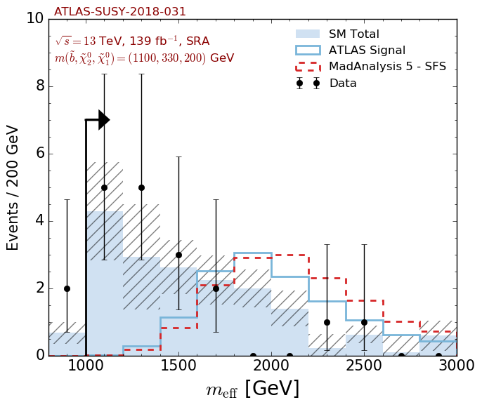
Figure 9.2: Histograms representative of the SRA cut-flow. We consider the distribution in the invariant mass of the reconstructed Higgs boson candidate (left) and in the effective mass (right), for a spectrum defined by $m(\tilde{b},\tilde{\chi}^{0}_{2},\tilde{\chi}^{0}_{1})=(1100,330,200)$ GeV. The dashed red line refers to the MadAnalysis 5 predictions, and the blue solid line to the ATLAS official results. As a reference, we show through solid blue bars matched with hatched areas the expected SM background and the related uncertainties, as well as the results emerging from data (black dots).

Our validation results are presented in a twofold way. First, we consider cut-flow tables for all scenarios and the signal region to which they are dedicated. Second, we present two histograms for each signal region, in which we compare differential distributions that are critical for each region. In our comparison, we use official results and digitised histogram information obtained from HEPData[132]. All cut-flow tables comprise two main columns, one for the ATLAS predictions and one for the MadAnalysis 5 ones. We provide the event counts surviving each cut, together with the relative cut efficiency ($\varepsilon$) and the $\delta$ difference between ATLAS and MadAnalysis 5 predictions. We also indicate the MC uncertainties after all requirements (for each bin in the case of the SRA and SRC regions). All tables have been prepared with the ma5_expert package [136].

In table 9.3.2 and figure 9.2, we consider the benchmark scenario that is defined by the mass spectrum $m(\tilde{b},\tilde{\chi}^{0}_{2},\tilde{\chi}^{0}_{1})=(1100,330,200)$ GeV and that probes the SRA class of regions. Investigating the cut-flow chart presented in the table, we observe a generally good agreement between our predictions and the official ATLAS results. The largest variations arise in the third and fourth bins in the effective mass $m_{\rm eff}$, with $\delta$ deviations reaching 26% and 23% respectively, for an ATLAS MC uncertainty $\Delta_{\rm MC}$ of about 7%–8%. We additionally observe a large MC uncertainty associated with the ATLAS predictions for the second $m_{\rm eff}$ bin, with $\Delta_{\rm MC}=29\%$, that is much larger than the difference between the ATLAS and MadAnalysis 5 predictions. This large MC uncertainty is also reflected through shifts in the $m_{\rm eff}$ distributions presented in figure 9.2 (right panel). In the left panel of the figure, we moreover show the invariant mass of the reconstructed Higgs boson candidate for which the ATLAS and MadAnalysis 5 numbers agree to a good level. In general, we thus observe a good agreement between the ATLAS and MadAnalysis 5 predictions, both at the cut-flow and differential distribution levels, after accounting for the sometimes quite large Monte Carlo uncertainties associated with the public ATLAS results.

Same as in table 9.3.2 but for the signal region SRB and a spectrum defined by $m(\tilde{b},\tilde{\chi}^{0}_{2},\tilde{\chi}^{0}_{1})=(700,680,550)$ GeV. The ATLAS results correspond to 3,527 MC events prior to any cut, whereas our predictions rely on 149,019 events. ATLAS MadAnalysis 5–SFS Events $\varepsilon$ Events $\varepsilon$ $\delta$ [%] Initial 2278.6 - 2278.6 - - Lepton veto 1482.6 0.651 1638.4 0.719 10.5 $N_{j}\geq 5$ 943.8 0.637 907.5 0.554 13.0 $N_{b}\geq 4$ 130.2 0.138 145.0 0.160 15.9 $\not{E}_{T}>350$ GeV 24.1 0.185 25.1 0.173 6.5 min$[\Delta\phi(j_{1-4},\not{E}_{T})]>0.4$ 12.8 0.531 12.8 0.510 3.9 Tau veto 12.8 1.000 12.6 0.982 1.8 $\bar{m}_{h}^{\rm reco}\in[75,175]$ GeV 8.5 0.664 7.0 0.559 15.8 Leading jet non-$b$-tagged 8.5 1.000 5.6 0.802 19.8 $p_{T}(j_{1})>350$ GeV 7.4 0.871 4.1 0.724 16.9 $|\Delta\phi(j_{1},\not{E}_{T})|>2.8$ 7.4 1.000 3.2 0.787 21.3 $m_{\rm eff}>1$ TeV 7.4 1.000 3.2 0.990 1.0 $\Delta_{\rm MC}/N_{\rm yield}$ $28.8\%$ $6.9\%$

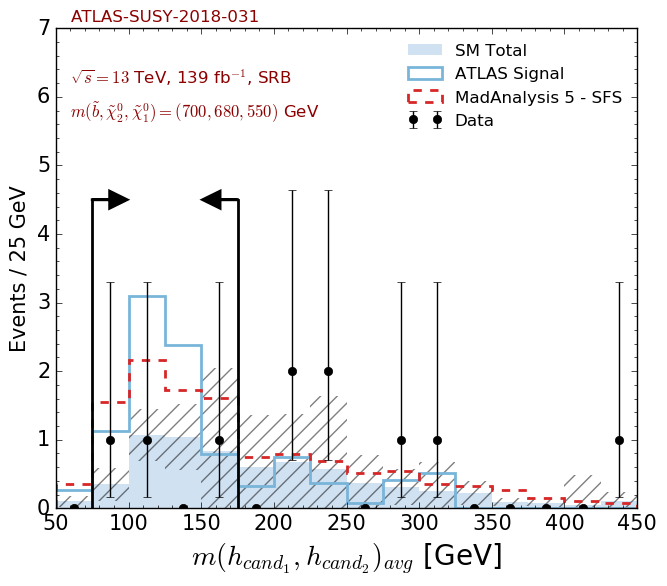
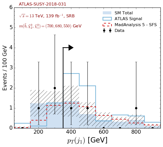
Figure 9.3: Histograms representative of the SRB cut-flow. We consider the distribution in the average invariant mass of the Higgs boson candidates (left) and in the $p_{T}$ of the leading jet (right), for a spectrum defined by $m(\tilde{b},\tilde{\chi}^{0}_{2},\tilde{\chi}^{0}_{1})=(700,680,550)$ GeV. The dashed red line refers to the MadAnalysis 5 predictions, and the blue solid line to the ATLAS official results. As a reference, we show through solid blue bars matched with hatched areas the expected SM background and the related uncertainties, as well as the results emerging from data (black dots).

Figure 9.4: Histograms representative of the SRC cut-flow. We consider the distribution in the missing transverse energy (left) and in its significance (right), for a spectrum defined by $m(\tilde{b},\tilde{\chi}^{0}_{2},\tilde{\chi}^{0}_{1})=(1200,1150,60)$ GeV. The dashed red line refers to the MadAnalysis 5 predictions, and the blue solid line to the ATLAS official results. As a reference, we show through solid blue bars matched with hatched areas the expected SM background and the related uncertainties, as well as the results emerging from data (black dots).

In table 9.3.2 and figure 9.3, we present results that are relevant for the validation of our implementation of the SRB region, and that have been computed in the context of the benchmark scenario defined by the mass spectrum $m(\tilde{b},\tilde{\chi}^{0}_{2},\tilde{\chi}^{0}_{1})=(700,680,550)$ GeV. In terms of the various cut efficiencies shown in table 9.3.2, we observe deviations $\delta$ between our MadAnalysis 5 predictions and the ATLAS official results that reach up to 21%. However, the ATLAS reference numbers are coming with a quite large MC uncertainty $\Delta_{\rm MC}$ of 28%. The situation is further emphasised in figure 9.3, in which we present in particular the transverse momentum distribution of the leading jet (right panel). The MadAnalysis 5 (red dashed lines) and ATLAS predictions indeed quite differ in the low $p_{T}$ regime that is relevant for the cut-flow. Focusing on the second distribution shown in the figure, one may be tempted to naively conclude that the shape of the $\bar{m}_{h}^{\rm reco}$ observable is on the contrary pretty well reproduced (left panel). The ATLAS curve however features fluctutations and quite differs from the MadAnalysis 5 results in the region that is relevant for the cut-flow. After accounting for the uncertainties on the ATLAS numbers, we cannot therefore draw any strong conclusion about the validation of our implementation. As the related MadAnalysis 5 code is similar to that relevant for the SRA and SRC regions for which good agreement is found (see above and below), we nevertheless consider our implementation as validated. The lack of publc information prevents us from investigating this problem more deeply.

In table 9.3.2 and figure 9.4, we finally turn to the validation of the implementation of the last class of signal regions, the SRC regions, for which we consider a benchmark scenario featuring $m(\tilde{b},\tilde{\chi}^{0}_{2},\tilde{\chi}^{0}_{1})=(1200,1150,60)$ GeV. Both our predictions and the official ATLAS numbers are here numerically accurate, $\Delta_{\rm MC}$ being small. Our predictions are found to agree quite well with the ATLAS predictions, both for the cut-flow tables, the $\not{E}_{T}$ spectrum and the missing transverse energy significance spectrum.

Same as in table 9.3.2 but for the signal region SRC and a spectrum defined by $m(\tilde{b},\tilde{\chi}^{0}_{2},\tilde{\chi}^{0}_{1})=(1200,1150,60)$ GeV. The ATLAS results correspond to 9,668 MC events prior to any cut, whereas our predictions rely on 64,305 events. ATLAS MadAnalysis 5–SFS Events $\varepsilon$ Events $\varepsilon$ $\delta$ [%] Initial 180.3 - 180.3 - - Lepton veto 127.5 0.707 129.6 0.719 1.7 $N_{j}\geq 4$ 117.1 0.918 120.8 0.932 1.5 $N_{b}\geq 3$ 67.9 0.580 61.9 0.513 11.6 $\not{E}_{T}>250$ GeV 61.5 0.906 56.3 0.910 0.5 min$[\Delta\phi(j_{1-4},\not{E}_{T})]>0.4$ 50.4 0.820 45.6 0.810 1.2 $\not{E}_{T}/\sqrt{H_{T}}>22\ \sqrt{\rm GeV}$ 26.7 0.530 26.3 0.577 9.0 $\Delta_{\rm MC}/N_{\rm yield}$ $2.2\%$ $1.1\%$ $\not{E}_{T}/\sqrt{H_{T}}\in[22,24]\ \sqrt{\rm GeV}$ 6.7 0.133 5.8 0.126 4.8 $\Delta_{\rm MC}/N_{\rm yield}$ $4.5\%$ $1.7\%$ $\not{E}_{T}/\sqrt{H_{T}}\in[24,26]\ \sqrt{\rm GeV}$ 6.4 0.127 5.8 0.126 0.7 $\Delta_{\rm MC}/N_{\rm yield}$ $4.7\%$ $1.7\%$ $\not{E}_{T}/\sqrt{H_{T}}>\in[26,28]\ \sqrt{\rm GeV}$ 5.5 0.109 5.1 0.112 2.9 $\Delta_{\rm MC}/N_{\rm yield}$ $5.5\%$ $1.9\%$ $\not{E}_{T}/\sqrt{H_{T}}>28\ \sqrt{\rm GeV}$ 8.2 0.163 8.1 0.178 9.2 $\Delta_{\rm MC}/N_{\rm yield}$ $4.9\%$ $1.2\%$

9.4 Conclusions

In this note, we presented our efforts on the implementation of the ATLAS-SUSY-2018-31 analysis in the MadAnalysis 5 framework, using the SFS detector simulation based on smearing and efficiency functions that is shipped with MadAnalysis 5. We have validated our work in the context of three simplified models dedicated to the production and decay of supersymmetric partners of the bottom quark. The validation has been achieved by comparing predictions obtained with our implementation to official results from the ATLAS collaboration. A reasonable agreement has been achieved for each signal region, the deviations remaining in general under a level of 20%–30%. The most considerable discrepancies can be traced to MC uncertainties inherent to the official ATLAS results, hindering hence our capacity to properly validate the implementation of one of the analysis signal regions. The good agreement obtained for all other regions, relying on the same piece of code, nevertheless makes us considering this analysis as validated.

The MadAnalysis 5 C++ code is available for download from the MadAnalysis 5 dataverse (https://doi.org/10.14428/DVN/IHALED) [29]. The material relevant for the validation benchmarks has been obtained from HEPData [132].

Acknowledgments

The authors are grateful to Laura Jeanty and Federico Meloni for their help with understanding the ATLAS analysis considered in this work. JYA has received funding from the European Union’s Horizon 2020 research and innovation programme as part of the Marie Sklodowska-Curie Innovative Training Network MCnetITN3 (grant agreement no. 722104).

10 Implementation of the ATLAS-SUSY-2018-32 analysis (sleptons and eletroweakinos with two leptons and missing transverse energy; 139 fb^-1)

By Jack Y. Araz and Benjamin Fuks

10.1 Introduction

Supersymmetry (SUSY) is one of the most popular extensions of the Standard Model (SM). By naturally extending the Poincaré algebra and linking the fermionic and bosonic degrees of freedom of the theory, SUSY could provide, among others, a solution for the hierarchy problem of the SM and an explanation for the problematics of dark matter. The so-called Minimal Supersymmetric Standard Model (MSSM) [123, 124] consists in the direct supersymmetrisation of the SM, giving thus rise to one SUSY partner to each SM degrees of freedom. In this framework, the slepton mass eigenstates are the superpartners of the SM leptons, and the electroweakino mass eigenstates consist of admixtures of the partners of the SM gauge and Higgs fields. More precisely, electroweakinos comprise the electrically-charged charginos ($\tilde{\chi}^{\pm}_{i},\ i\in 1,2$) and the electrically-neutral neutralinos ($\tilde{\chi}^{0}_{i},\ i\in 1,2,3,4$). The lightest neutralino is often considered to be the lightest supersymmetric particle (LSP), hence a potentially viable candidate for dark matter.

The ATLAS-SUSY-2018-32 analysis [30] has been structured to look for new physics signals that might appear due to charginos and sleptons. It searches for dilepton and missing energy final states which can emerge from the production of either a pair of lightest charginos, or of a pair of sleptons. Two separate benchmarks have been constructed for this purpose in the chargino case. First, a pure wino-like ($\tilde{W}$) chargino is considered to decay into a bino-like ($\tilde{B}$) LSP and a lepton via an intermediate $W$-boson. Second, the same wino-like chargino is assumed to cascade decay to the same final state, but this time through a slepton exchange. Additionally, a third benchmark scenario is dedicated to the pair production of sleptons that decay each into a lepton and an LSP. Those three cases are illustrated with the Feynman diagrams of Fig. 10.1.

Those three scenarios have been analysed to constrain the corresponding simplified models. The experimental results have shown that for a massless LSP, chargino masses up to 420 GeV are excluded at $95\%$ confidence level (CL) in the first class of scenarios (chargino pair production and decay via a charged weak gauge boson). A more severe bound has been set on the second class of scenarios, when charginos decay through an intermediate slepton. The masses are in this case constrained to be larger than 1 TeV at $95\%$ CL. Finally, slepton mass bounds, as derived in the context of the third class of scenarios, are of 700 GeV.

In the rest of this note, we present the recast of ATLAS-SUSY-2018-32 analysis of Ref. [Aad:2019vnb] in the MadAnalysis 5 framework, that is now available from the MadAnalysis 5 Public Analysis Database and the MadAnalysis 5 dataverse [31].

10.2 Description of the analysis

This analysis targets a signature made of two lepton and missing transverse energy, as could arise from the production and decay of a pair lightest charginos ($\tilde{\chi}^{\pm}_{1}$) or slepton ($\tilde{l}_{i}$). As mentioned in the previous section, the results are interpreted in three classes of simplified models depicted in the diagrams of Fig 10.1. The first two of these extend the SM by a chargino and a neutralino LSP, the difference between them lying at the level of the chargino decay. In the first setup, charginos decay into a single lepton and missing energy via an intermediate $W$-boson, whereas in the second setup, they decay via an intermediate slepton. In the last class of simplified models under consideration, the SM is supplemented by a charged slepton and a neutralino LSP, the slepton being taken directly decaying into the LSP and a lepton. The validation of our re-implementation is achieved in these three cases.

Figure 10.1: Representative Feynman diagrams for the scenarios used for the validation of our re-implementation of the ATLAS-SUSY-2018-32 analysis. We consider chargino production followed by decays through electroweak bosons (left), slepton production followed by direct decays into leptons and missing energy (centre) and chargino production followed by decays mediated by an intermediate slepton or sneutrino (right). The diagrams have been taken from Ref. [30].

10.2.1 Object definitions

Jets are obtained by the clustering all participants to the hadronic activity in the event, electrons and photons according to the anti-$k_{T}$ algorithm [42], as embedded in the FastJet package version 3.3.3 [43], with a radius parameter set to $R=0.4$. Jet candidates are then extracted by requiring the reconstructed objects to have a minimum transverse momentum $p_{T}>20$ GeV and a pseudorapidity satistying $|\eta|<2.4$.

Electron and muons are required to satisfy strong isolation conditions to be considered as a signal leptons.

A signal electron is required to have a minimum $p_{T}$ of 10 GeV and to be within $|\eta|<2.47$. These electrons are then required to be isolated from the calorimetric activity and any other charged track. This is achieved in practice by constraining the sum of the $p_{T}$ of all tracks lying in a cone of radius $\Delta R$ around the electron to be smaller than 15% of the electron transverse momentum, the cone radius being defined by $\Delta R=\min(10/p_{T},0.2)$. Moreover, the calorimetric activity, $I^{e}_{rel}$, in a cone of radius $\Delta R=0.2$ around the electron is restricted to be smaller than 20% of the electron $p_{T}$. For very hard electrons with $p_{T}>200$ GeV, a special isolation treatment is, however, implemented. In this case, one solely imposes the signal electron to be calorimetrically isolated, requiring $I^{e}_{rel}<{\rm max}(0.015p_{T},3.5)$.

Signal muons are defined similarly. Their transverse momentum is imposed to fulfil $p_{T}>10$ GeV and their pseudorapidity $|\eta|<2.7$. Track-based isolation implies that the sum of the transverse momentum of all tracks lying in a cone of radius $\Delta R={\rm min}(10/p_{T},0.3)$ around the muon is smaller than 15% of the muon transverse momentum, whilst calorimetric isolation enforces $I^{\mu}_{rel}<0.3p_{T}$, for a cone of radius $\Delta R=0.2$ centred on the muon.

Finally, all jets at a distance in the transverse plane of $\Delta R\leq 0.2$ (0.4) of an electron (muon) are removed, and all electrons are required to be separated from any muon by least $\Delta R=0.2$. The collection of $b$-jets is extracted from the collection of cleaned signal jets.

10.2.2 Event selection

The considered ATLAS-SUSY-2018-32 analysis includes four sets of signal regions differing by the properties of the dilepton system and the jet activity in the event. Two categories of signal regions feature a pair of leptons of different flavours (DF). Regions of the first class impose a veto to the presence of any final-state signal jet, whereas regions of the second sub-category allow for the presence of one jet in the final state. Similarly, two classes of regions are designed to probe final states featuring a pair of leptons of the same flavour (SF), these two sub-categories differing by requiring either zero or one final-state jet.

After dedicated pre-selection requirements, all signal regions are further divided into different bins in the $m_{T2}$ observable defined by [114, 115]

$$m_{T2}(\mathbf{p}_{T,1},\mathbf{p}_{T,2},\mathbf{p}^{\rm miss}_{T})=\min\limits_{\mathbf{q}_{T,1}+\mathbf{q}_{T,2}=\mathbf{p}^{\rm miss}_{T}}\left\{\max\left[m_{T}(\mathbf{p}_{T,1},\mathbf{q}_{T,1}),m_{T}(\mathbf{p}_{T,2},\mathbf{q}_{T,2})\right]\right\}\ .$$

Here $\mathbf{p}_{T,1}$ and $\mathbf{p}_{T,2}$ are transverse momentum vectors of the two leptons and $\mathbf{q}_{T,1}$ and $\mathbf{q}_{T,2}$ are chosen to be a decomposition of the missing momentum vector, $\mathbf{q}_{T,1}+\mathbf{q}_{T,2}=\mathbf{p}^{\rm miss}_{T}$. A minimisation is performed over all possible decompositions of the missing momentum vector. For each decomposition, we calculate the transverse mass of the system constitued by the first (second) lepton and the $\mathbf{q}_{T,1}$ ($\mathbf{q}_{T,2}$) vector. The $m_{T2}$ value is then taken as the minimum of the maximum of the two transverse masses associated with a given $\mathbf{p}^{\rm miss}_{T}$ decomposition.

In order to take trigger efficiencies into account, events are reweighed by 85% before any selection requirement. All signal regions then imposes that events feature two opposite-sign leptons with a minimum transverse momentum of 25 GeV, and whose invariant ,ass is larger than 25 GeV. A $b$-jet veto is further enforced. At this stage, the analysis is split into four categories, as mentioned above (DF/SF lepton pair, with or without one jet).

The DF signal regions additionally asks that the invariant mass of the lepton pair satisfies $m_{l_{1},l_{2}}>100$ GeV, whereas the SF ones increase this threshold to $m_{l_{1},l_{2}}>121.2$ GeV. Finally, all signal regions require the presence of at least 100 GeV of missing transverse energy, and the missing energy significance, defined by $\not{E}_{T}/\sqrt{H_{T}}$, has to be larger than 10 $\sqrt{\rm GeV}$. In this expression, the denominator involves the $H_{T}$ variable that consists of the scalar sum of the transverse momenta of all signal jets. A schematic representation of all signal regions is shown in Table 10.2.2.

Schematic representation of the ATLAS-SUSY-2018-32 signal region definitions. Different Flavour (DF) Same Flavour (SF) OS dilep. with $p^{l_{1},l_{2}}_{T}>25$ [GeV] $m_{l_{1},l_{2}}>25$ [GeV] b veto DF dilep. & $N_{j}=0$ DF dilep. & $N_{j}=1$ SF dilep. & $N_{j}=0$ SF dilep. & $N_{j}=1$ $m_{l_{1},l_{2}}>100$ [GeV] $m_{l_{1},l_{2}}>121.2$ [GeV] $\not{E}_{T}>110$ [GeV] $\not{E}_{T}$ Sig. $>10$ [$\sqrt{\rm GeV}$] $m_{T2}$ bins

10.3 Validation

10.3.1 Event generation

For the validation of the re-implementation of the ATLAS-SUSY-2018-32 analysis, we study the three different scenarios defined above. For the production of a pair of charginos that both decay via a $W$-boson, we choose a mass spectrum such that $m(\tilde{\chi}^{\pm}_{1},\tilde{\chi}^{0}_{1})=(300,50)$ GeV, all other SUSY states being decoupled. Similarly, for the scenario focusing on slepton pair production, we choose $m(\tilde{l}^{\pm},\tilde{\chi}^{0}_{1})=(400,200)$ GeV and decouple the rest of the spectrum. Finally, for the scenario where the two pair-produced charginos decay via an intermediate slepton, the mass spectrum is chosen to be $m(\tilde{\chi}^{\pm}_{1},\tilde{l}^{\pm},\tilde{\chi}^{0}_{1})=(600,300,1)$ GeV, with again all other superpartners being decoupled. All SLHA spectrum files can be found in dedicated HEPData records provided by the ATLAS collaboration [137].

For our validation, we generate various leading-order event samples with MG5_aMC version 2.7.3 [48]. Following the MLM prescription [117], we merge samples featuring up to two extra jets at the matrix-element level, the merging scale being set to one quarter of the mass of the pair-produced SUSY particle. All events are showered and hadronised by means of Pythia 8 [51], and the simulation of the ATLAS detector is performed with the Delphes 3 package [9]. Through our simulation we used the leading-order set of NNPDF 2.3 parton distribution functions, as provided by LhaPDF [133, 50]. Our re-implementation can then be used to investigate the ATLAS-SUSY-2018-32 sensitivity to the simulated signals, through MadAnalysis 5 version 1.8 (or more recent) [8]. All analysis files can be obtained from the MadAnalysis 5 Public Analysis Database [3].

10.3.2 Comparison with the official results

In this section we compare our preductions for all the benchmarks described in section 10.3.1 with the corresponding official ATLAS results. To estimate the quality of our re-implementation, we define a variable $\delta$ to quantify the difference between the relative cut efficiencies as obtained from the ATLAS and MadAnalysis 5 results,

$$\delta_{i}=\frac{|\varepsilon^{\rm ATLAS}_{i}-\varepsilon^{\rm MA5}_{i}|}{\varepsilon^{\rm ATLAS}_{i}}\ .$$

Here $\varepsilon_{i}$ represents the relative cut efficiency which is defined as $\varepsilon_{i}=N_{i}/N_{i-1}$, $N_{i}$ being number of surviving events after the $i^{\rm th}$ cut. The analysis will be considered as validated provided that all $\delta_{i}$ values are found to satisfy $\delta\lesssim 20\%$. In the present recast exercise, it should be noted that the lack of public information related to how the ATLAS collaboration has prepared its Monte Carlo production introduces a certain bias and makes the comparison complicated.

Finally, in order to evaluated the statistical power associated with our event generation procedure, we quantify the Monte Carlo uncertainty through a $\Delta_{\rm MC}$ quantity defined by

$$\Delta_{\rm MC}=\frac{N_{n}}{\sqrt{N^{\rm MC}_{n}}}\ ,$$

where $N^{\rm MC}_{n}$ is defined by the number of unweighted Monte Carlo events surviving the last cut. In our validation, we aim to remain a $10\%$ Monte Carlo uncertainty, that is found to always be smaller than the magnitude of the deviation between the MadAnalysis 5 predsictions and the ATLAS results after the last cut.

Our results include a comparison between MadAnalysis 5 predictions and ATLAS official results for all four considered classes of signal regions, that respectively target the production of a SF lepton pair with 0 jet, the production of a SF lepton pair with 1 jet, the production of a DF lepton pair with 0-jet and the production of a DF lepton pair with 1 jet. As only ATLAS predictions for the $m_{T2}\in[100,\infty[$ GeV bin are available in HEPData, we accordingly restrict the discussion to this sole inclusive bin.

Tables LABEL:tab:sf_cha and LABEL:tab:df_cha include cut-flow results for the benchmark simplified model featuring chargino production and decay via a $W$-boson. As can be seen in the lower panel of table LABEL:tab:df_cha, the largest variation from the ATLAS results has been observed to be $20.3\%$ for the $\not{E}_{T}$ significance requirement. This disagreement stems from potentially genuine differences between the implementation of this cut in our re-implementation and in the non-public ATLAS code. However, our definition still gives a reasonably acceptable deviation from the ATLAS results, especially after accounting for all other cuts.

We then present results for slepton production (third class of benchmarks) in table LABEL:tab:sf_slep, and for chargino pair-production followed by chargino decays via an intermediate slepton (second class of benchmarks) in tables LABEL:tab:sf_chaslep and LABEL:tab:df_chaslep.

Tables LABEL:tab:sf_cha–LABEL:tab:df_chaslep comprise two main columns, one for the ATLAS results and one for the MadAnalysis 5 ones. These columns are further divided, so that they include the number of events surviving each cut, the relative cut efficiencies and the $\delta_{i}$ quantities for each cut. All tables have been prepared with the ma5_expert package [136].

Cut-flow associated with the signal region dedicated to the production of a SF lepton pair without any jet (upper) or with a single jet (lower), for a benchmark scenario of the first category (production of a pair of charginos that decay each via a $W$-boson), for a spectrum defined by $m(\tilde{\chi}^{\pm}_{1},\tilde{\chi}^{0}_{1})=(300,50)$ GeV.

Figure 13.1: Validation figures of our implementation, in the MadAnalysis 5 framework, of the CMS four-top analysis of Ref. [36]. We compare MadAnalysis 5 predictions (green) with the CMS official results (dark grey) for the jet multiplicity (upper-left panel), $b$-jet multiplicity (upper-right panel) and $H_{T}$ (central-left panel) spectra, as well as for the event counts populating each signal region (lower right panel). The MadAnalysis 5 predictions include theoretical uncertainties (green error bars) whilst the CMS numbers include both systematical and statistical errors (black dashed bands and light grey error bars in the lower panel).

13.4 A practical example: top-philic scalars

As a simple illustrative example, we consider a simplified ($SU(2)$-violating) model in which a top-philic real scalar $S$ of mass $M_{S}$ interacts with the Standard Model through the top-quark. The corresponding new physics Lagrangian reads

$$\mathcal{L}_{s0}\supset\frac{1}{2}\partial_{\mu}S\partial^{\mu}S-\frac{1}{2}M_{S}^{2}S^{2}+y_{0}\bar{t}t\ S+h.c\ ,$$ (13.9)

where $y_{0}$ denotes the new Yukawa coupling. The main production mechanism of the four-top signal induced by new physics, when $M_{S}>2m_{t}$ and $M_{S}$ is around or below the TeV-scale proceeds via associated production,

$$pp\to t\bar{t}S\to t\bar{t}t\bar{t}\ .$$ (13.10)

For lower scalar masses, the on-shell production of the scalar $S$ dominates, implying that the cross section scales as $y_{0}^{2}$. On the contrary, for higher mass, the off-shell contribution dominates instead, so that the cross section scales as $y_{0}^{4}$.

We present in Table 13.4 limits on the new physics signal cross section that we derive with our MadAnalysis 5 implementation. We consider two scenarios in which $M_{S}=600$ GeV and $M_{S}=1000$ GeV respectively, and show results for each SR of the analysis. We observe that the strongest limits arise for the SR4, SR5 and SR8 region. The lack of sensitivity of the SR6 region is associated with an observed large upward fluctuation of events in CMS data. We moreover present projections for the HL-LHC as derived with the machinery introduced in Ref. [84].

Observed and limits on the considered new physics signal production rate, as obtained with MadAnalysis 5 and by using the implementation of the CMS-TOP-18-003 analysis [36]. We consider two scenarios for which $M_{S}=600$ GeV (upper row) and $M_{S}=1000$ GeV (lower row). We moreover also show the projected limits at the HL-LHC. SR1 SR2 SR3 SR4 SR5 SR6 SR7 SR8 SR9 SR10 SR11 SR12 SR13 SR14 $M_{S}=600~{}\rm{GeV}$ $~{}\sigma^{\rm{lim}}_{\rm{obs}}$ (fb) $86$ $70$ $124$ $55$ $29$ $97$ $49$ $\mathbf{23}$ $169$ $363$ $979$ $87$ $95$ $80$ $~{}\sigma^{\rm{lim}}_{\rm{HL-LHC}}$ (fb) $26$ $29$ $34$ $19$ $\mathbf{13}$ $16$ $19$ $12$ $58$ $65$ $351$ $26$ $23$ $21$ $M_{S}=1000~{}\rm{GeV}$ $~{}\sigma^{\rm{lim}}_{\rm{obs}}$ (fb) $74$ $49$ $61$ $50$ $25$ $74$ $25$ $\mathbf{17}$ $125$ $175$ $189$ $100$ $78$ $45$ $~{}\sigma^{\rm{lim}}_{\rm{HL-LHC}}$ (fb) $22$ $20$ $17$ $17$ $11$ $12$ $10$ $\mathbf{9}$ $43$ $32$ $68$ $30$ $18$ $13$

Next, we scan over the singlet mass in the $[400,1200]$ GeV range, and translate the limits on the cross section as a direct constraint on the $S$ coupling to the top quark. We remind that $t\bar{t}S$ associated production typically dominates for such mass values. We present limits derived from the CMS analysis under consideration (blue), as well as projections for the HL-LHC (green) in Fig. 13.2. The regions above the blue and green thick line in the figure correspond to a 95% confidence level exclusion by the CMS-TOP-18-003 analysis when considering the run 2 and HL-LHC luminosity respectively. In order to derive these limits, we use standard build-in features from MadAnalysis 5 allowing for the calculation of the exclusion confidence level associated with a given signal. These are extensively documented in ref. [8]. The large error bars (corresponding to the shaded regions in the figure) are related to the significant theoretical uncertainties associated with our leading-order signal simulations. We refer to ref. [176] for a more refined analysis.

Figure 13.2: Limit on $y_{0}$ as a function of masses derived from the above procedure in MadAnalysis 5  along with projections for the HL-LHC based on $3$ ab^-1 of data. The regions above the curves are excluded, and the shaded areas show the associated theoretical uncertainties for both limits.

At face value, the additional statistics provided by the HL-LHC imply a $50\%$ improvements in the limits. However, the new physics signal is expected to strongly deviate from the SM background in various observables, such as the sum of the transverse momenta of all reconstructed jets $H_{T}$. One can therefore expect a significant improvement on these limits from a dedicated search strategy, as already mentioned in Ref. [170].

13.5 Conclusions

We have described in this work the implementation of the CMS-TOP-18-003 analysis in the MadAnalysis 5 framework. Such an analysis can be used to target new physics expected to show up in four-top events at LHC. We have validated our work by comparing predictions relying on the Monte Carlo simulations of SM four-top production. We have found an agreement with the CMS official results, well within their $1\sigma$ uncertainties. In particular, all the SR event counts agree with the CMS $t\bar{t}t\bar{t}$ projection within $~{}30\%$, as do the differential distributions in $H_{T}$, $N_{\rm jets}$ and $N_{b}$. Consequently, the present work can be considered as validated and used without restriction to probe and test novel new physics models.

As an illustrative example of usage, we have reintepreted the CMS-TOP-18-003 analysis to extract bounds on a simplified top-philic scalar model, together with their projection at the HL-LHC.

The MadAnalysis 5 C++ recast code is available online from the MA5 dataverse (https://doi.org/10.14428/DVN/OFAE1G) [37].

Acknowledgments

LD is supported by the INFN “Iniziativa Specifica” Theoretical Astroparticle Physics (TAsP-LNF).

References

- [1] C. K. Khosa, S. Kraml, A. Lessa, P. Neuhuber and W. Waltenberger, LHEP 158, 2020 (5 2020), arXiv:2005.00555 [hep-ph].
- [2] M. Drees, H. Dreiner, D. Schmeier, J. Tattersall and J. S. Kim, Comput. Phys. Commun. 187, 227 (2015), arXiv:1312.2591 [hep-ph].
- [3] B. Dumont, B. Fuks, S. Kraml, S. Bein, G. Chalons, E. Conte, S. Kulkarni, D. Sengupta and C. Wymant, Eur. Phys. J. C 75, 56 (2015), arXiv:1407.3278 [hep-ph].
- [4] A. Buckley, J. Butterworth, L. Lonnblad, D. Grellscheid, H. Hoeth, J. Monk, H. Schulz and F. Siegert, Comput. Phys. Commun. 184, 2803 (2013), arXiv:1003.0694 [hep-ph].
- [5] GAMBIT Collaboration, C. Balázs et al., Eur. Phys. J. C 77, 795 (2017), arXiv:1705.07919 [hep-ph].
- [6] E. Conte, B. Fuks and G. Serret, Comput. Phys. Commun. 184, 222 (2013), arXiv:1206.1599 [hep-ph].
- [7] E. Conte, B. Dumont, B. Fuks and C. Wymant, Eur. Phys. J. C 74, 3103 (2014), arXiv:1405.3982 [hep-ph].
- [8] E. Conte and B. Fuks, Int. J. Mod. Phys. A 33, 1830027 (2018), arXiv:1808.00480 [hep-ph].
- [9] DELPHES 3 Collaboration, J. de Favereau, C. Delaere, P. Demin, A. Giammanco, V. Lemaître, A. Mertens and M. Selvaggi, JHEP 02, 057 (2014), arXiv:1307.6346 [hep-ex].
- [10] J. Y. Araz, B. Fuks and G. Polykratis (6 2020), arXiv:2006.09387 [hep-ph].
- [11] S. Kraml et al., Eur. Phys. J. C 72, 1976 (2012), arXiv:1203.2489 [hep-ph].
- [12] LHC Reinterpretation Forum Collaboration, W. Abdallah et al. (3 2020), arXiv:2003.07868 [hep-ph].
- [13] B. Fuks et al. (6 2018), arXiv:1806.02537 [hep-ph].
- [14] ATLAS Collaboration, G. Aad et al., Phys. Rev. D 100, 052013 (2019), arXiv:1906.05609 [hep-ex].
- [15] K. Park, S. Lee, W. Jun and U. Min, https://doi.org/10.14428/DVN/GLWLTF (2020).
- [16] CMS Collaboration, A. M. Sirunyan et al., Phys. Lett. B 795, 76 (2019), arXiv:1811.10151 [hep-ex].
- [17] B. Fuks and A. Jueid, https://doi.org/10.14428/DVN/ICOXG9 (2020).
- [18] CMS Collaboration, A. M. Sirunyan et al., Phys. Rev. D 99, 012010 (2019), arXiv:1810.10092 [hep-ex].
- [19] Y. Kang, J. Kim, J. Choi and S. Yun, 10.14428/DVN/GAZACQ (2020).
- [20] CMS Collaboration, A. M. Sirunyan et al., JHEP 03, 051 (2020), arXiv:1911.04968 [hep-ex].
- [21] E. Conte and R. Ducrocq, 10.14428/DVN/DTYUUE (2021).
- [22] CMS Collaboration, A. M. Sirunyan et al., Phys. Lett. B 795, 398 (2019), arXiv:1812.06359 [hep-ex].
- [23] J.-B. Lee and J. Lee, https://doi.org/10.14428/DVN/UOH6BF (2020).
- [24] ATLAS Collaboration, G. Aad et al., Phys. Rev. D 101, 032009 (2020), arXiv:1911.06660 [hep-ex].
- [25] J. Lim, C.-T. Lu, J.-H. Park and J. Park, 10.14428/DVN/UN3NND (2020).
- [26] ATLAS Collaboration, G. Aad et al., Phys. Rev. D 101, 072001 (2020), arXiv:1912.08479 [hep-ex].
- [27] J. Kim, T. G. Lee, J. Kim and H. Jang, https://doi.org/10.14428/DVN/LYQMUJ (2020).
- [28] ATLAS Collaboration, G. Aad et al., JHEP 12, 060 (2019), arXiv:1908.03122 [hep-ex].
- [29] B. Fuks and J. Y. Araz, 10.14428/DVN/IHALED (2020).
- [30] ATLAS Collaboration, G. Aad et al., Eur. Phys. J. C 80, 123 (2020), arXiv:1908.08215 [hep-ex].
- [31] B. Fuks and J. Y. Araz, https://doi.org/10.14428/DVN/EA4S4D (2020).
- [32] ATLAS Collaboration, G. Aad et al. (2020), arXiv:1909.09226 [hep-ex].
- [33] M. Goodsell, 10.14428/DVN/BUN2UX (2020).
- [34] CMS Collaboration, A. M. Sirunyan et al., JHEP 10, 244 (2019), arXiv:1908.04722 [hep-ex].
- [35] M. Malte, S. Bein and J. Sonneveld, https://doi.org/10.14428/DVN/4DEJQM (2020).
- [36] CMS Collaboration, A. M. Sirunyan et al., Eur. Phys. J. C 80, 75 (2020), arXiv:1908.06463 [hep-ex].
- [37] L. Darmé and B. Fuks, https://doi.org/10.14428/DVN/OFAE1G (2020).
- [38] G. Altarelli, B. Mele and M. Ruiz-Altaba, Z. Phys. C 45, 109 (1989), [Erratum: Z.Phys.C 47, 676 (1990)].
- [39] B. Fuks and R. Ruiz, JHEP 05, 032 (2017), arXiv:1701.05263 [hep-ph].
- [40] ATLAS Collaboration, G. Aad et al., JINST 14, P12006 (2019), arXiv:1908.00005 [hep-ex].
- [41] ATLAS Collaboration, G. Aad et al., Eur. Phys. J. C 76, 292 (2016), arXiv:1603.05598 [hep-ex].
- [42] M. Cacciari, G. P. Salam and G. Soyez, JHEP 04, 063 (2008), arXiv:0802.1189 [hep-ph].
- [43] M. Cacciari, G. P. Salam and G. Soyez, Eur. Phys. J. C 72, 1896 (2012), arXiv:1111.6097 [hep-ph].
- [44] M. Cacciari and G. P. Salam, Phys. Lett. B 641, 57 (2006), arXiv:hep-ph/0512210.
- [45] A. Alloul, N. D. Christensen, C. Degrande, C. Duhr and B. Fuks, Comput. Phys. Commun. 185, 2250 (2014), arXiv:1310.1921 [hep-ph].
- [46] J. Alwall, R. Frederix, S. Frixione, V. Hirschi, F. Maltoni, O. Mattelaer, H. S. Shao, T. Stelzer, P. Torrielli and M. Zaro, JHEP 07, 079 (2014), arXiv:1405.0301 [hep-ph].
- [47] P. Artoisenet, R. Frederix, O. Mattelaer and R. Rietkerk, JHEP 03, 015 (2013), arXiv:1212.3460 [hep-ph].
- [48] J. Alwall, C. Duhr, B. Fuks, O. Mattelaer, D. G. Öztürk and C.-H. Shen, Comput. Phys. Commun. 197, 312 (2015), arXiv:1402.1178 [hep-ph].
- [49] R. D. Ball et al., Nucl. Phys. B 867, 244 (2013), arXiv:1207.1303 [hep-ph].
- [50] A. Buckley, J. Ferrando, S. Lloyd, K. Nordström, B. Page, M. Rüfenacht, M. Schönherr and G. Watt, Eur. Phys. J. C 75, 132 (2015), arXiv:1412.7420 [hep-ph].
- [51] T. Sjöstrand, S. Ask, J. R. Christiansen, R. Corke, N. Desai, P. Ilten, S. Mrenna, S. Prestel, C. O. Rasmussen and P. Z. Skands, Comput. Phys. Commun. 191, 159 (2015), arXiv:1410.3012 [hep-ph].
- [52] J. L. Feng, S. Su and F. Takayama, Phys. Rev. Lett. 96, 151802 (2006), arXiv:hep-ph/0503117.
- [53] A. Birkedal, K. Matchev and M. Perelstein, Phys. Rev. D 70, 077701 (2004), arXiv:hep-ph/0403004.
- [54] Y. Bai, P. J. Fox and R. Harnik, JHEP 12, 048 (2010), arXiv:1005.3797 [hep-ph].
- [55] P. J. Fox, R. Harnik, J. Kopp and Y. Tsai, Phys. Rev. D 84, 014028 (2011), arXiv:1103.0240 [hep-ph].
- [56] N. F. Bell, J. B. Dent, A. J. Galea, T. D. Jacques, L. M. Krauss and T. J. Weiler, Phys. Rev. D 86, 096011 (2012), arXiv:1209.0231 [hep-ph].
- [57] A. A. Petrov and W. Shepherd, Phys. Lett. B 730, 178 (2014), arXiv:1311.1511 [hep-ph].
- [58] Y. Bai and T. M. Tait, Phys. Lett. B 723, 384 (2013), arXiv:1208.4361 [hep-ph].
- [59] J. Andrea, B. Fuks and F. Maltoni, Phys. Rev. D 84, 074025 (2011), arXiv:1106.6199 [hep-ph].
- [60] ATLAS Collaboration, M. Aaboud et al., JHEP 06, 059 (2016), arXiv:1604.01306 [hep-ex].
- [61] ATLAS Collaboration, M. Aaboud et al., Phys. Rev. D 94, 032005 (2016), arXiv:1604.07773 [hep-ex].
- [62] ATLAS Collaboration, M. Aaboud et al., Phys. Lett. B 763, 251 (2016), arXiv:1608.02372 [hep-ex].
- [63] ATLAS Collaboration, M. Aaboud et al., Phys. Lett. B 765, 11 (2017), arXiv:1609.04572 [hep-ex].
- [64] ATLAS Collaboration, M. Aaboud et al., Eur. Phys. J. C 77, 393 (2017), arXiv:1704.03848 [hep-ex].
- [65] ATLAS Collaboration, M. Aaboud et al., Phys. Rev. D 96, 112004 (2017), arXiv:1706.03948 [hep-ex].
- [66] ATLAS Collaboration, M. Aaboud et al., Phys. Rev. Lett. 119, 181804 (2017), arXiv:1707.01302 [hep-ex].
- [67] ATLAS Collaboration, M. Aaboud et al., Phys. Lett. B 776, 318 (2018), arXiv:1708.09624 [hep-ex].
- [68] ATLAS Collaboration, M. Aaboud et al., Eur. Phys. J. C 78, 18 (2018), arXiv:1710.11412 [hep-ex].
- [69] ATLAS Collaboration, M. Aaboud et al., JHEP 01, 126 (2018), arXiv:1711.03301 [hep-ex].
- [70] ATLAS Collaboration, M. Aaboud et al., JHEP 10, 180 (2018), arXiv:1807.11471 [hep-ex].
- [71] CMS Collaboration, A. M. Sirunyan et al., JHEP 07, 014 (2017), arXiv:1703.01651 [hep-ex].
- [72] CMS Collaboration, A. M. Sirunyan et al., JHEP 10, 180 (2017), arXiv:1703.05236 [hep-ex].
- [73] CMS Collaboration, A. Sirunyan et al., Eur. Phys. J. C 77, 845 (2017), arXiv:1706.02581 [hep-ex].
- [74] CMS Collaboration, A. Sirunyan et al., Eur. Phys. J. C 78, 291 (2018), arXiv:1711.00431 [hep-ex].
- [75] CMS Collaboration, A. M. Sirunyan et al., Phys. Rev. D 97, 092005 (2018), arXiv:1712.02345 [hep-ex].
- [76] CMS Collaboration, A. M. Sirunyan et al., JHEP 06, 027 (2018), arXiv:1801.08427 [hep-ex].
- [77] CMS Collaboration, A. M. Sirunyan et al., JHEP 09, 046 (2018), arXiv:1806.04771 [hep-ex].
- [78] CMS Collaboration, A. M. Sirunyan et al., Phys. Rev. Lett. 122, 011803 (2019), arXiv:1807.06522 [hep-ex].
- [79] CMS Collaboration, A. M. Sirunyan et al., Eur. Phys. J. C 79, 280 (2019), arXiv:1811.06562 [hep-ex].
- [80] CMS Collaboration, A. M. Sirunyan et al., JHEP 03, 141 (2019), arXiv:1901.01553 [hep-ex].
- [81] CMS Collaboration, A. M. Sirunyan et al., JHEP 03, 025 (2020), arXiv:1908.01713 [hep-ex].
- [82] CMS Collaboration, A. M. Sirunyan et al. (8 2020), arXiv:2008.04735 [hep-ex].
- [83] M. J. Baker et al., JHEP 12, 120 (2015), arXiv:1510.03434 [hep-ph].
- [84] J. Y. Araz, M. Frank and B. Fuks, Eur. Phys. J. C 80, 531 (2020), arXiv:1910.11418 [hep-ph].
- [85] CMS Collaboration, A. Sirunyan et al., JINST 13, P06015 (2018), arXiv:1804.04528 [physics.ins-det].
- [86] CMS Collaboration, V. Khachatryan et al., JINST 10, P06005 (2015), arXiv:1502.02701 [physics.ins-det].
- [87] CMS Collaboration, A. Sirunyan et al., JINST 13, P10005 (2018), arXiv:1809.02816 [hep-ex].
- [88] CMS Collaboration, A. Sirunyan et al., JINST 13, P05011 (2018), arXiv:1712.07158 [physics.ins-det].
- [89] C. Borschensky, B. Fuks, A. Kulesza and D. Schwartländer, Phys. Rev. D 101, 115017 (2020), arXiv:2002.08971 [hep-ph].
- [90] R. Barbier et al., Phys. Rept. 420, 1 (2005), arXiv:hep-ph/0406039.
- [91] CDF Collaboration, T. Aaltonen et al., Phys. Rev. Lett. 107, 042001 (2011), arXiv:1105.2815 [hep-ex].
- [92] R. Dalitz, Phys. Rev. 94, 1046 (1954).
- [93] C. Degrande, C. Duhr, B. Fuks, D. Grellscheid, O. Mattelaer and T. Reiter, Comput. Phys. Commun. 183, 1201 (2012), arXiv:1108.2040 [hep-ph].
- [94] B. Fuks, Int. J. Mod. Phys. A 27, 1230007 (2012), arXiv:1202.4769 [hep-ph].
- [95] NNPDF Collaboration, R. D. Ball et al., JHEP 04, 040 (2015), arXiv:1410.8849 [hep-ph].
- [96] M. Redi, V. Sanz, M. de Vries and A. Weiler, JHEP 08, 008 (2013), arXiv:1305.3818 [hep-ph].
- [97] K. S. Agashe, J. Collins, P. Du, S. Hong, D. Kim and R. K. Mishra, JHEP 05, 078 (2017), arXiv:1612.00047 [hep-ph].
- [98] C. Biggio and F. Bonnet, Eur. Phys. J. C 72, 1899 (2012), arXiv:1107.3463 [hep-ph].
- [99] M. Casolino, T. Farooque, A. Juste, T. Liu and M. Spannowsky, Eur. Phys. J. C 75, 498 (2015), arXiv:1507.07004 [hep-ph].
- [100] W.-F. Chang, T. Modak and J. N. Ng, Phys. Rev. D 97, 055020 (2018), arXiv:1711.05722 [hep-ph].
- [101] CMS Collaboration, https://doi.org/10.17182/hepdata.91969 (2020).
- [102] CMS Collaboration, V. Khachatryan et al., Eur. Phys. J. C 76, 155 (2016), arXiv:1512.00815 [hep-ex].
- [103] E. Maguire, L. Heinrich and G. Watt, J. Phys. Conf. Ser. 898, 102006 (2017), arXiv:1704.05473 [hep-ex].
- [104] https://cms-project-generators.web.cern.ch/cms-project-generators/ .
- [105] CMS Collaboration, A. M. Sirunyan et al., Eur. Phys. J. C 80, 4 (2020), arXiv:1903.12179 [hep-ex].
- [106] U. Ellwanger, C. Hugonie and A. M. Teixeira, Phys. Rept. 496, 1 (2010), arXiv:0910.1785 [hep-ph].
- [107] M. Dine, W. Fischler and M. Srednicki, Phys. Lett. B 104, 199 (1981).
- [108] J. E. Kim and H. P. Nilles, Phys. Lett. B 138, 150 (1984).
- [109] D. Curtin et al., Phys. Rev. D 90, 075004 (2014), arXiv:1312.4992 [hep-ph].
- [110] CMS Collaboration, S. Chatrchyan et al., JINST 7, P10002 (2012), arXiv:1206.4071 [physics.ins-det].
- [111] CMS Collaboration, V. Khachatryan et al., JINST 12, P02014 (2017), arXiv:1607.03663 [hep-ex].
- [112] ATLAS Collaboration, 10.17182/hepdata.92006.v2 (2020).
- [113] ATLAS Collaboration, ATLAS-CONF-2017-029 (2017).
- [114] C. Lester and D. Summers, Phys. Lett. B 463, 99 (1999), arXiv:hep-ph/9906349.
- [115] H.-C. Cheng and Z. Han, JHEP 12, 063 (2008), arXiv:0810.5178 [hep-ph].
- [116] C. Duhr and B. Fuks, Comput. Phys. Commun. 182, 2404 (2011), arXiv:1102.4191 [hep-ph].
- [117] M. L. Mangano, M. Moretti, F. Piccinini and M. Treccani, JHEP 01, 013 (2007), arXiv:hep-ph/0611129.
- [118] J. Alwall, S. de Visscher and F. Maltoni, JHEP 02, 017 (2009), arXiv:0810.5350 [hep-ph].
- [119] ATLAS Collaboration, ATL-PHYS-PUB-2014-021 (2014).
- [120] B. Fuks, M. Klasen, D. R. Lamprea and M. Rothering, Eur. Phys. J. C 73, 2480 (2013), arXiv:1304.0790 [hep-ph].
- [121] B. Fuks, M. Klasen, D. R. Lamprea and M. Rothering, JHEP 01, 168 (2014), arXiv:1310.2621 [hep-ph].
- [122] A. L. Read, J. Phys. G28, 2693 (2002), [,11(2002)].
- [123] H. P. Nilles, Phys. Rept. 110, 1 (1984).
- [124] H. E. Haber and G. L. Kane, Phys. Rept. 117, 75 (1985).
- [125] P. Jackson, C. Rogan and M. Santoni, Phys. Rev. D 95, 035031 (2017), arXiv:1607.08307 [hep-ph].
- [126] P. Jackson and C. Rogan, Phys. Rev. D 96, 112007 (2017), arXiv:1705.10733 [hep-ph].
- [127] ATLAS Collaboration, M. Aaboud et al., Phys. Rev. D 98, 092012 (2018), arXiv:1806.02293 [hep-ex].
- [128] ATLAS Collaboration, G. Aad et al., Eur. Phys. J. C 79, 970 (2019), arXiv:1907.05120 [hep-ex].
- [129] ATLAS Collaboration, G. Aad et al., https://doi.org/10.17182/hepdata.91127.v2 (2020).
- [130] E. Witten, Nucl. Phys. B 188, 513 (1981).
- [131] R. Barbieri and G. Giudice, Nucl. Phys. B 306, 63 (1988).
- [132] ATLAS Collaboration, 10.17182/hepdata.89408.v2 (2019).
- [133] NNPDF Collaboration, R. D. Ball, V. Bertone, S. Carrazza, L. Del Debbio, S. Forte, A. Guffanti, N. P. Hartland and J. Rojo, Nucl. Phys. B 877, 290 (2013), arXiv:1308.0598 [hep-ph].
- [134] B. Fuks, M. Klasen, D. R. Lamprea and M. Rothering, JHEP 10, 081 (2012), arXiv:1207.2159 [hep-ph].
- [135] J. Butterworth et al., J. Phys. G 43, 023001 (2016), arXiv:1510.03865 [hep-ph].
- [136] J. Y. Araz, https://github.com/jackaraz/ma5_expert (2020).
- [137] ATLAS Collaboration, 10.17182/hepdata.89413 (2020).
- [138] ATLAS Collaboration, HepData record, https://www.hepdata.net/record/ins1755298.
- [139] D. R. Tovey, JHEP 04, 034 (2008), arXiv:0802.2879 [hep-ph].
- [140] G. Polesello and D. R. Tovey, JHEP 03, 030 (2010), arXiv:0910.0174 [hep-ph].
- [141] N. D. Christensen, P. de Aquino, C. Degrande, C. Duhr, B. Fuks, M. Herquet, F. Maltoni and S. Schumann, Eur. Phys. J. C 71, 1541 (2011), arXiv:0906.2474 [hep-ph].
- [142] L. Lönnblad and S. Prestel, JHEP 03, 166 (2013), arXiv:1211.7278 [hep-ph].
- [143] J. Debove, B. Fuks and M. Klasen, Nucl. Phys. B 842, 51 (2011), arXiv:1005.2909 [hep-ph].
- [144] J. Fiaschi and M. Klasen, Phys. Rev. D 98, 055014 (2018), arXiv:1805.11322 [hep-ph].
- [145] Heinrich, Lukas and Feickert, Matthew and Stark, Giordon, pyhf: v0.5.3, https://doi.org/10.5281/zenodo.1169739 (2020).
- [146] G. Alguero, S. Kraml and W. Waltenberger (9 2020), arXiv:2009.01809 [hep-ph].
- [147] M. D. Goodsell, S. Kraml, H. Reyes-González and S. L. Williamson, SciPost Phys. 9, 047 (2020), arXiv:2007.08498 [hep-ph].
- [148] CMS Collaboration, Search for supersymmetry in proton-proton collisions at 13 TeV in final states with jets and missing transverse momentum (2019).
- [149] T. Sjostrand, S. Mrenna and P. Z. Skands, Comput. Phys. Commun. 178, 852 (2008), arXiv:0710.3820 [hep-ph].
- [150] R. Frederix, D. Pagani and M. Zaro, JHEP 02, 031 (2018), arXiv:1711.02116 [hep-ph].
- [151] CMS Collaboration, A. M. Sirunyan et al., Eur. Phys. J. C 78, 140 (2018), arXiv:1710.10614 [hep-ex].
- [152] ATLAS Collaboration, M. Aaboud et al., JHEP 12, 039 (2018), arXiv:1807.11883 [hep-ex].
- [153] M. Battaglia and G. Servant, Nuovo Cim. C 033N2, 203 (2010), arXiv:1005.4632 [hep-ex].
- [154] N. Greiner, K. Kong, J.-C. Park, S. C. Park and J.-C. Winter, JHEP 04, 029 (2015), arXiv:1410.6099 [hep-ph].
- [155] E. Alvarez, D. A. Faroughy, J. F. Kamenik, R. Morales and A. Szynkman, Nucl. Phys. B 915, 19 (2017), arXiv:1611.05032 [hep-ph].
- [156] J. H. Kim, K. Kong, S. J. Lee and G. Mohlabeng, Phys. Rev. D 94, 035023 (2016), arXiv:1604.07421 [hep-ph].
- [157] P. J. Fox, I. Low and Y. Zhang, JHEP 03, 074 (2018), arXiv:1801.03505 [hep-ph].
- [158] B. Lillie, J. Shu and T. M. Tait, JHEP 04, 087 (2008), arXiv:0712.3057 [hep-ph].
- [159] A. Pomarol and J. Serra, Phys. Rev. D 78, 074026 (2008), arXiv:0806.3247 [hep-ph].
- [160] N. Zhou, D. Whiteson and T. M. Tait, Phys. Rev. D 85, 091501 (2012), arXiv:1203.5862 [hep-ph].
- [161] G. Cacciapaglia, H. Cai, A. Deandrea, T. Flacke, S. J. Lee and A. Parolini, JHEP 11, 201 (2015), arXiv:1507.02283 [hep-ph].
- [162] G. Cacciapaglia, A. Deandrea, T. Flacke and A. Iyer, JHEP 05, 027 (2020), arXiv:2002.01474 [hep-ph].
- [163] P. J. Fox, A. E. Nelson and N. Weiner, JHEP 08, 035 (2002), arXiv:hep-ph/0206096.
- [164] T. Plehn and T. M. Tait, J. Phys. G 36, 075001 (2009), arXiv:0810.3919 [hep-ph].
- [165] S. Choi, M. Drees, J. Kalinowski, J. Kim, E. Popenda and P. Zerwas, Phys. Lett. B 672, 246 (2009), arXiv:0812.3586 [hep-ph].
- [166] D. Goncalves-Netto, D. Lopez-Val, K. Mawatari, T. Plehn and I. Wigmore, Phys. Rev. D 85, 114024 (2012), arXiv:1203.6358 [hep-ph].
- [167] S. Calvet, B. Fuks, P. Gris and L. Valery, JHEP 04, 043 (2013), arXiv:1212.3360 [hep-ph].
- [168] K. Benakli, M. Goodsell, F. Staub and W. Porod, Phys. Rev. D 90, 045017 (2014), arXiv:1403.5122 [hep-ph].
- [169] W. Kotlarski, JHEP 02, 027 (2017), arXiv:1608.00915 [hep-ph].
- [170] L. Darmé, B. Fuks and M. Goodsell, Phys. Lett. B 784, 223 (2018), arXiv:1805.10835 [hep-ph].
- [171] M. Gerbush, T. J. Khoo, D. J. Phalen, A. Pierce and D. Tucker-Smith, Phys. Rev. D 77, 095003 (2008), arXiv:0710.3133 [hep-ph].
- [172] A. Hayreter and G. Valencia, Phys. Rev. D 96, 035004 (2017), arXiv:1703.04164 [hep-ph].
- [173] ATLAS Collaboration, M. Aaboud et al., Phys. Rev. D 97, 112001 (2018), arXiv:1712.02332 [hep-ex].
- [174] E. Alvarez, A. Juste and R. M. S. Seoane, JHEP 12, 080 (2019), arXiv:1910.09581 [hep-ph].
- [175] CMS Collaboration, V. Khachatryan et al., Eur. Phys. J. C 76, 439 (2016), arXiv:1605.03171 [hep-ex].
- [176] L. Darmé, B. Fuks and F. Maltoni, To appear .