Uniqueness of non-trivial spherically symmetric black hole solution in special classes of ${\textit{F}(R)}$ gravitational theory

Abstract

We show, in detail, that the only non-trivial black hole (BH) solutions for a neutral as well as a charged spherically symmetric space-times, using the class ${\textit{F}(R)}={\textit{R}}\pm{\textit{F}_{1}(R)}$, must-have metric potentials in the form $h(r)=\frac{1}{2}-\frac{2M}{r}$ and $h(r)=\frac{1}{2}-\frac{2M}{r}+\frac{q^{2}}{r^{2}}$. These BHs have a non-trivial form of Ricci scalar, i.e., $R=\frac{1}{r^{2}}$ and the form of ${\textit{F}_{1}(R)}=\mp\frac{\sqrt{\textit{R}}}{3M}$. We repeat the same procedure for (Anti-)de Sitter, (A)dS, space-time and got the metric potentials of neutral as well as charged in the form $h(r)=\frac{1}{2}-\frac{2M}{r}-\frac{2\Lambda r^{2}}{3}$ and $h(r)=\frac{1}{2}-\frac{2M}{r}+\frac{q^{2}}{r^{2}}-\frac{2\Lambda r^{2}}{3}$, respectively. The Ricci scalar of the (A)dS space-times has the form ${\textit{R}}=\frac{1+8r^{2}\Lambda}{r^{2}}$ and the form of ${\textit{F}_{1}(R)}=\mp\frac{\textit{2}\sqrt{R-8\Lambda}}{3M}$. We calculate the thermodynamical quantities, Hawking temperature, entropy, quasi-local energy, and Gibbs-free energy for all the derived BHs, that behaves asymptotically as flat and (A)dS, and show that they give acceptable physical thermodynamical quantities consistent with the literature. Finally, we prove the validity of the first law of thermodynamics for those BHs.

I Introduction

To describe the early and late cosmic epoch of our universe consistently, scientists invented the modified gravitational theories that contain higher-order curvature expressions. Such expressions are responsible to make the theories renormalizable which means that they are quantizable theories of gravitation Stelle (1977). Moreover, such theories are interesting to teach us how to understand the presence of dark matter and confront such theories with observation Nojiri and Odintsov (2006); Copeland et al. (2006); Nojiri and Odintsov (2011); Awad et al. (2018a); Clifton et al. (2012); Tang et al. (2019); Awad et al. (2018b). At the beginning of the formulation of modified gravitational theories, different constructions have been done that involve all the second-order curvature scalar Podolsky et al. (2018); Lü et al. (2015); Bueno and Cano (2017, 2016). Additionally, there was a particular class that contains the higher-order curvature invariants that constructed from the Ricci scalar De Felice and Tsujikawa (2010); Cognola et al. (2008, 2008); Pogosian and Silvestri (2008, 2010); Zhang (2006); Li and Barrow (2007); Song et al. (2007); Nojiri and Odintsov (2008, 2007); Capozziello et al. (2018); Vainio and Vilja (2017); Ostrogradsky (1850). In spite that ${\textit{F}(R)}$ theories prevent the existence of any other invariants except Ricci scalar they can also prevent the existence of Ostrogradskis instability Ostrogradsky (1850) that is a feature of higher derivative theories Woodard (2007).

The simplest modification of general relativity (GR) is to include $R^{d}$, $d>0$, to Einstein Hilbert action and the output field equations are able to discuss the inflationary epoch Starobinsky (1980). Also, we can consider the term $R^{d}$, $d<0$, which can discuss the behavior of the universe at the late epoch Carroll et al. (2003, 2004); Capozziello (2002); Capozziello et al. (2003). In ${\textit{F}(R)}$ gravitational theory, one can reproduce BHs that are compatible or different from GR Multamaki and Vilja (2006); Nashed (2018a); Multamaki and Vilja (2007); de la Cruz-Dombriz et al. (2009); Nashed (2018b); Hendi et al. (2012); Nashed (2018); Sebastiani and Zerbini (2011). A spherically symmetric BHs which are different from GR have been derived form a special class of ${\textit{F}(R)}$, i.e., ${\textit{F}(R)=R-2\alpha\sqrt{R}}$ Nashed and Capozziello (2019); Elizalde et al. (2020); Nashed et al. (2020). These BHs have non-trivial Ricci scalar that has the form $\frac{1}{r^{2}}$. In this study, we are going to prove that such BHs are unique for the special class ${\textit{F}(R)=R\pm{\textit{F}_{1}(R)}}$.

In (2019) the event horizon telescope picked up the first image of a BH, at the center of the galaxy Messier 87 Akiyama et al. (2019). Since then the interest in BH studies have increased rapidly. This image was a real test of the Einstein GR theory. Moreover, the image of BH brings observations closer to the event horizon in contrast to what has been done before as a test of GR by looking at the motions of stars and gas clouds near the edge of a BH. The picked image confirmed a dark shadow-like region, caused by gravitational bending and capture of light which was predicted by Einstein GR Falcke et al. (2000). In this study, we show that our BH solution is a unique correction to GR modulating the shape and the size of the event horizon. By a fine measurement, improving the precision, one could discriminate between GR and $f(R)$ BH solutions. For example, if we have a corrected BH solution of GR, like what we have done in this study, discrimination between the two models, GR and $f(R)$, could be available. We would stress that the precision of shadow measurements could select the theory.

The plan of this study is the following. In Sec. II a summary of Maxwell-${\textit{F}(R)}$ gravity is given. In Sec. III, restricting to spherically symmetric space-time, exactly neutral as well as charged BH solutions of the field equations of ${\textit{F}(R)}$ are derived in detail. In Sec. IV, the same calculations are performed for the neutral and charged cases for which the field equations contain a cosmological constant, and BH solutions are derived. These BHs behave asymptotically as (A)dS space-time. In Sec. V, we calculate the thermodynamic quantities like entropy, Hawking temperature, and quasi-local energy to all BHs derived in Sec. III and Sec. IV and show that all the resulting thermodynamic quantities are physically acceptable. Finally, we show in Sec. V that the first law of thermodynamics is satisfied for the BHs derived in Sec. III and Sec. IV. In the final section, Sec. VI, we discuss the main results of the present study, figured out some convincing conclusions, and investigate some ideas for future study.

II A brief summary of the Maxwell–${\textit{F}(R)}$ theory

${\textit{F}(R)}$ gravitational theory is a modification of GR that is studied early by many authors (cf. Carroll et al. (2004); Buchdahl (1970); Nojiri and Odintsov (2003); Capozziello et al. (2003); Capozziello and De Laurentis (2011); Nojiri and Odintsov (2011); Nojiri et al. (2017); Capozziello (2002)). The Lagrangian of Maxwell–${\textit{F}(R)}$ theory takes the form:

$${\mathop{\mathcal{L}}}_{g}:=\frac{1}{2\kappa}\int d^{4}x\sqrt{-g}\Big{[}{\textit{F}(R)}-\Lambda-\frac{1}{2}\mathrm{f}^{2}\Big{]}\equiv\frac{1}{2\kappa}\int d^{4}x\sqrt{-g}\Big{[}{\textit{R}+F_{1}(R)}-\Lambda-\frac{1}{2}\mathrm{f}^{2}\Big{]},$$ (1)

where R is the Ricci scalar, $\kappa$ is the gravitational constant, $\Lambda$ is the cosmological constant, $g$ is the determinant of the metric, and ${\textit{F}_{1}(R)}$ is an arbitrary function that can take any form. Equation (1) shows that when ${\textit{F}_{1}(R)}\neq 0$ we have a theory deviates from GR. In Eq. (1), $\mathrm{f}^{2}=\mathrm{f}_{\mu\nu}\mathrm{f}^{\mu\nu}$ and $\mathrm{f}_{\mu\nu}=\mathrm{A}_{\mu,\nu}-\mathrm{A}_{\nu,\mu}$, where $\mathrm{A}_{\mu}$ is the gauge potential and the comma means ordinary differentiation.

Making variations of the Lagrangian (1) w.r.t. the metric tensor $g_{\mu\nu}$ and the strength tensor $\mathrm{f}$, respectively, we can write the field equations of the Maxwell–${\textit{F}(R)}$ gravitational theory as Cognola et al. (2005)

$${\textit{E}}_{\mu\nu}={\textit{R}}_{\mu\nu}\Big{[}{\textit{1}+F_{1}(R)}\Big{]}-\frac{1}{2}g_{\mu\nu}\Big{[}{\textit{R}+F_{1}(R)}\Big{]}-2g_{\mu\nu}\Lambda+g_{\mu\nu}\Box{\textit{F}}_{{}_{\textit{1}R}}-\nabla_{\mu}\nabla_{\nu}{\textit{F}}_{{}_{\textit{1}R}}-8\pi{\textit{T}_{\mu\nu}}\equiv 0,$$ (2)

$${\partial}_{\nu}\left(\sqrt{-{\textit{g}}}\,{\mathrm{f}}^{\mu\nu}\right)=0,$$ (3)

where $\Box$ is the d’Alembertian operator, $\displaystyle{\textit{F}}_{{}_{\textit{1}R}}=\frac{dF_{1}({\textit{R}})}{d{\textit{R}}}$ and the energy-momentum tensor, ${\textit{T}_{\mu\nu}}$, is defined as

$${\textit{T}_{\mu\nu}}:=\frac{1}{4\pi}\left({\textit{g}}_{\rho\sigma}{{\mathrm{f}}_{\nu}{}^{\rho}}{{{\mathrm{f}}}_{\mu}}^{\sigma}-\displaystyle{1\over 4}{\textit{g}}_{\mu\nu}\mathrm{f}^{2}\right).$$ (4)

The trace of Eq. (2), takes the form

$${\textit{E}}={\textit{R}}{\textit{F}}_{\textit{1}R}-2{\textit{F}(R)}-8\Lambda+3\Box{\textit{F}}_{\textit{1}R}=0\,.$$ (5)

Equation (5) has no contribution from the electromagnetic part due to the skewness of this part. In the following section, we are going to apply the field equations (2), (3) and (5), with/without charged and with/without cosmological constant for a particular form of spherically symmetric space-time.

III Black holes with asymptotic flatness

In this section, we are going to apply the neutral and charged field equations (2), (3) and (5) without the cosmological constant to a spherically symmetric space-time and try to derive a general form of the arbitrary function ${\textit{F}_{1}(R)}$.

III.1 A neutral BH with asymptote flat space-time

It is well known that in the frame of GR any neutral spherically symmetric solution of the metric

$$ds^{2}=-h(r)dt^{2}+\frac{dr^{2}}{h(r)}+r^{2}(d\theta^{2}+\sin^{2}d\phi^{2}),$$ (6)

has the following form

$$h(r)=1-\frac{2M}{r}\,,$$ (7)

where $M$ is the gravitational mass of the BH. Equation (6) with Eq. (7) has a vanishing Ricci scalar, i.e., ${\textit{R}}=0$, and therefore can be a solution to ${\textit{F}(R)}$ gravitational theory. However, when

$$h(r)=\frac{1}{2}-\frac{2M}{r}\,,$$ (8)

the Ricci scalar becomes not trivial, i.e., ${\textit{R}}=\frac{1}{r^{2}}$ and the metric (6) will be a solution to the class ${\textit{F}(R)}={\textit{R}}-2\alpha\sqrt{{\textit{R}}}$ where $M=\frac{1}{6\alpha}$ Nashed and Capozziello (2019). In this section, we are going to search if there is any other non-trivial solution in the frame of ${\textit{F}(R)}$ gravitational theory. For this purpose we assume that the metric potential to have the form

$$h(r)=\xi-\frac{2M}{r}\,,$$ (9)

where $\xi$ is an arbitrary real parameter. Equation (9) coincides with Eqs. (6) and (8) when $\xi=1$ and $\xi=1/2$ respectively. The Ricci scalar of the metric (6) using Eq. (9) has the form

$${\textit{R}(r)}=\frac{2(1-\xi)}{r^{2}}\Rightarrow{\textit{r}(R)}=\pm\frac{2(1-\xi)}{\sqrt{\textit{R}}}.$$ (10)

Applying the field equations (2) and (5) to Eq. (6) using the metric potential (9) we get the following system of non-linear differential equations

$${\textit{E}}_{t}{}^{t}=\frac{1}{2r^{2}}\left(2\,\xi-2-\mathbb{F}{r}^{2}\right)+\frac{{r}^{2}\left(r\xi-2\,M\right)\mathbb{F}^{\prime\prime\prime}-{r}\left(15\,M-8\,{r}\xi\right)\mathbb{F}^{\prime\prime}-3\left(7\,M-4\,{r}\xi\right)\mathbb{F}^{\prime}}{4\left(\xi-1\right)}=0\,,$$

$${\textit{E}}_{r}{}^{r}=\frac{1}{2r^{2}}\left(2\,\xi-2-\mathbb{F}{r}^{2}\right)-\frac{{r}\left(3\,M-2\,{r}\xi\right)\mathbb{F}^{\prime\prime}+3\left(3\,M-2\,{r}\xi\right)\mathbb{F}^{\prime}}{4\left(\xi-1\right)}=0\,,$$

$${\textit{E}}_{\theta}{}^{\theta}=E_{\phi}{}^{\phi}=-\frac{\mathbb{F}}{2}+\frac{{r}^{2}\left({r}\xi-2\,M\right)\mathbb{F}^{\prime\prime\prime}-r\left(12\,M-7\,\xi\,{r}\right)\mathbb{F}^{\prime\prime}+\left[\left(8\,\xi+1\right)r-12\,M\right]\mathbb{F}^{\prime}}{4(\xi-1)}=0\,,$$

$${\textit{E}}=\frac{2}{r^{2}}\left(\xi-1-\mathbb{F}{r}^{2}\right)+\frac{3{r}^{2}\left(\,{r}\xi-2\,M\right)\mathbb{F}^{\prime\prime\prime}-6{r}\left(7\,M-4\,{r}\xi\right)\mathbb{F}^{\prime\prime}+2\left[\left(17\,\xi+1\right){r}-27\,M\right]\mathbb{F}^{\prime}}{4\left(\xi-1\right)}=0\,,$$ (11)

where $\mathbb{F}^{\prime}=\frac{d\mathbb{F}(r)}{dr}$, $\mathbb{F}^{\prime\prime}=\frac{d^{2}\mathbb{F}(r)}{dr^{2}}$, $\mathbb{F}^{\prime\prime\prime}=\frac{d^{3}\mathbb{F}(r)}{dr^{3}}$, ${\textit{F}_{1}(R(r))}=\mathbb{F}\equiv\mathbb{F}(r)$ and $\frac{\textit{d}F_{1}(R(r))}{d\textit{(}R(r))}=\frac{d\mathbb{F}(r)}{dr}\frac{dr}{d\textit{(}R(r))}$. Equation (11) informs us that when $\mathbb{F}=0$ then $\xi=1$. In that case, $\mathbb{F}=0$, there will be no new solution different from the well-known solution of GR as it should be because ${\textit{R}}=0$ as is clear from Eq. (10). Assuming that $\mathbb{F}\neq 0$ and $\xi\neq 1$ we get the following two solutions of the system (11):

$$\xi=1+\frac{c_{1}}{2},\qquad\qquad{\textrm{a}nd}\qquad\qquad\mathbb{F}(r)=\frac{c_{1}}{r^{2}}\,,$$

$$\xi=\frac{1}{2},\qquad\qquad\qquad{\textrm{a}nd}\qquad\qquad\mathbb{F}(r)=\frac{1}{3Mr}\,.$$ (12)

Using Eq. (10) in the first set of Eq. (III.1) we get

$${\textit{F}(R)}\propto{\textit{R}}\qquad\qquad{\textrm{w}hich\,\,is\,\,the\,\,case\,\,of\,\,GR}$$ (13)

while if we use Eq. (10) in the second set of Eq. (III.1) we get

$${\textit{F}(R)}={\textit{R}}\mp\frac{\sqrt{\textit{R}}}{3M}.$$ (14)

Equation (14) shows that for the metric potential (9) the only non-charged BH solution that can deviates from GR comes from the contribution of ${\textit{F}_{1}(R)}$ that has the only following form

$${\textit{F}_{1}(R)}=\mp\frac{\sqrt{\textit{R}}}{3M},$$ (15)

where $\xi=1/2$. Equation (15) coincides with that derived in Nashed and Capozziello (2019); Nashed et al. (2020) when $M=\frac{1}{6\alpha}$. Now we are going to study the charged form of ${\textit{F}(R)}$ and see what is the form of ${\textit{F}_{1}(R)}$ in that case.

III.2 Charged BH with asymptotic flatness

It is well-know that the charged BH solution in the frame of GR has a metric potential in the form

$$h(r)=1-\frac{2M}{r}+\frac{q^{2}}{r^{2}}\,,$$ (16)

where $q$ is the charge parameter which comes from the electromagnetic potential $\mathrm{A}$ that comes from the definition $\mathrm{f}_{\mu\nu}=\mathrm{A}_{\mu,\nu}-\mathrm{A}_{\nu,\mu}$ where the vector $\mathrm{A}_{\mu}$ has the form $\mathrm{A}=(q/r,0,0,0)$ Reissner (1916). Equation (16) has a vanishing Ricci scalar. However, when

$$h(r)=\frac{1}{2}-\frac{2M}{r}+\frac{q^{2}}{r^{2}}\,,$$ (17)

the Ricci scalar is not trivial and takes the form $R=\frac{1}{r^{2}}$ and the metric (16) will be a solution to the class ${\textit{F}(R)}={\textit{R}}-2\alpha\sqrt{{\textit{R}}}$ Nashed and Capozziello (2019). Now, assuming the metric potential to have the form

$$h(r)=\xi_{1}-\frac{2M}{r}+\frac{q^{2}}{r^{2}}\,,$$ (18)

where $\xi_{1}$ is an arbitrary real parameter. Applying the field equations (2), (3) and (5) to Eq. (6) using the metric potential (18) we get the following system of non-linear differential equations

$${\textit{E}}_{t}{}^{t}=\frac{1}{2r^{2}}\left(2\,\xi-2-\mathbb{F}{r}^{2}\right)+\frac{\left(\xi_{1}-\frac{2\,M}{r}+\frac{{q}^{2}}{r^{2}}\right){r}^{3}\mathbb{F}^{\prime\prime\prime}+\left(8\,\xi_{1}-\frac{15\,M}{r}+7\,\frac{{q}^{2}}{r^{2}}\right){r}^{2}\mathbb{F}^{\prime\prime}+\left(8\,\frac{{q}^{2}}{r^{2}}-\frac{21\,M}{r}+12\,\xi_{1}\,\right){r}\mathbb{F}^{\prime}}{4\left(\xi_{1}-1\right)}=0\,,$$

$${\textit{E}}_{r}{}^{r}=\frac{1}{2r^{2}}\left(2\,\xi-2-\mathbb{F}{r}^{2}\right)+\frac{\left(2\,\xi_{1}-\frac{3\,M}{r}+\frac{{q}^{2}}{r^{2}}\right){r}^{2}\mathbb{F}^{\prime\prime}+\left(6\,\xi_{1}-\frac{9\,M}{r}+2\,\frac{{q}^{2}}{r^{2}}\right){r}\mathbb{F}^{\prime}}{4\left(\xi_{1}-1\right)}=0\,,$$

$${\textit{E}}_{\theta}{}^{\theta}=E_{\phi}{}^{\phi}=\frac{-\mathbb{F}}{2}+\frac{\left(\xi_{1}-\frac{2\,M}{r}+\frac{{q}^{2}}{r^{2}}\right){r}^{3}\mathbb{F}^{\prime\prime\prime}+\left(7\,\xi_{1}-\frac{12\,M}{r}+5\,\frac{{q}^{2}}{r^{2}}\right){r}^{2}\mathbb{F}^{\prime\prime}+\left(\left(8\,\xi_{1}+1\right)-\frac{12\,M}{r}+4\,\frac{{q}^{2}}{r^{2}}\right){r}\mathbb{F}^{\prime}}{4\left(\xi_{1}-1\right)}=0\,,$$

$${\textit{E}}=\frac{2}{r^{2}}\left(\xi-1-\mathbb{F}{r}^{2}\right)+\frac{3\left(\xi_{1}-\frac{2\,M}{r}+\,\frac{{q}^{2}}{r^{2}}\right){r}^{3}\mathbb{F}^{\prime\prime\prime}+6\left(4\,\xi_{1}-\frac{7\,\,M}{r}+3\,\frac{{q}^{2}}{r^{2}}\right){r}^{2}\mathbb{F}^{\prime\prime}+2\left(\left(1+17\,\xi_{1}\right)-\frac{27\,M}{r}+9\,\frac{{q}^{2}}{r^{2}}\right)r\mathbb{F}^{\prime}}{4\left(\xi_{1}-1\right)}=0.$$

(19)

Equations (19) reduce to Eqs. (11) when the charge parameter $q=0$. Also Eqs. (19) indicate that when $\mathbb{F}=0$ we get $\xi_{1}=1$ and similar discussion carried out for the neutral BH can also apply to the charged case. Solving system (19) assuming that $\mathbb{F}\neq 0$ and $\xi_{1}\neq 1$ we get the following solution

$$\xi_{1}=\frac{1}{2},\qquad\qquad{\textrm{a}nd}\qquad\qquad\mathbb{F}(r)=\frac{1}{3Mr}\,.$$ (20)

Equation (20) indicates that all the results obtained in the neutral case will be identical with the charged case. We must stress on the fact that in the charged case the charge parameter $q$ has no effect on the form of ${\textit{F}_{1}(R)}$ because the term $q/r^{2}$ is a solution to the GR field equation so its effect disappears in the higher order curvature terms.

IV Black holes with asymptotic (ANTI-)DE-space-time

We have shown in the previous section that the only non-trivial solution, that behaves asymptotically as flat space-time, in ${\textit{F}(R)}$ gravitational theory must have a metric potential in the form $\frac{1}{2}-\frac{2M}{r}$ for the neutral case and $\frac{1}{2}-\frac{2M}{r}+\frac{q^{2}}{r^{2}}$ for the charged one. Those solutions give a non-trivial form of the Ricci scalar, ${\textit{R}=\frac{1}{r^{2}}}$, and the form of ${\textit{F}_{1}(R)}$ is ${\textit{F}_{1}(R)}=\mp\frac{\sqrt{{\textit{R}}}}{3M}$. In this section we are going to follow the same technique of the previous section and study neutral and charged BHs that behave asymptotically as (A)dS using the line-element (6).

IV.1 Non-charged BH with asymptotic (A)dS

Taking the metric potential to have the form

$$h(r)=\xi_{2}-\frac{2M}{r}+\xi_{3}r^{2}\,,$$ (21)

where $\xi_{2}$ and $\xi_{3}$ are arbitrary real parameters. The Ricci scalar of the metric (6) using Eq. (21) has the form

$${\textit{R}(r)}=\frac{2(1-\xi_{2}-6\xi_{3}r^{2})}{r^{2}}\Rightarrow{\textit{r}(R)}=\pm\frac{\sqrt{2(1-\xi_{2})}}{\sqrt{\textit{(}R+12\xi_{3})}}.$$ (22)

Equation (22) shows that when $\xi_{2}=1$ and $\xi_{3}=0$ we get a vanishing Ricci scalar which corresponds to a flat space-time BH solution of GR. Therefore, for non-constant Ricci scalar we must choose any value for $\xi_{2}$ except 1. Applying the field equations (2) and (5) to Eq. (6) using the metric potential (21) we get the following system of non-linear differential equations

$${\textit{E}}_{t}{}^{t}=\frac{1}{r^{2}}\left(\left[{2\Lambda}-\frac{\mathbb{F}{r}^{2}}{2}+3{\xi_{3}}\right]{r}^{2}+\xi_{2}-1\right)+\frac{1}{4\left(\xi_{2}-1\right)}\Bigg{\{}\left(r\xi_{2}-{2\,M}+{r}^{3}{\xi_{3}}\right){r}^{2}\mathbb{F}^{\prime\prime\prime}+\left(9\,{r}^{3}{\xi_{3}}-{15\,M}+8r\,\xi_{2}\right){r}\mathbb{F}^{\prime\prime}$$

$$+3\left(4r\xi_{2}-{7\,M}+4{r}^{3}{\xi_{3}}\right)\mathbb{F}^{\prime}\Bigg{\}}=0\,,$$

$${\textit{E}}_{r}{}^{r}=\frac{1}{r^{2}}\left(\left[{2\Lambda}-\frac{\mathbb{F}{r}^{2}}{2}+3{\xi_{3}}\right]{r}^{2}+\xi_{2}-1\right)+\frac{\left(2r\xi_{2}-{3\,M}+3\,{r}^{3}{\xi_{3}}\right){r}\mathbb{F}^{\prime\prime}+3\left(2\,{r}^{3}{\xi_{3}}-{3\,M}+2r\,\xi_{2}\right){r}\mathbb{F}^{\prime}}{4\left(\xi_{2}-1\right)}=0\,,$$

$${\textit{E}}_{\theta}{}^{\theta}=E_{\phi}{}^{\phi}=\left(2\,{\Lambda}-\frac{\mathbb{F}}{2}+3{\xi_{3}}\right)+\frac{1}{4\,(\xi_{2}-1)}\Bigg{\{}\left(r\xi_{2}-{2\,M}+{r}^{3}{\xi_{3}}\right){r}^{2}\mathbb{F}^{\prime\prime\prime}+\left(9\,{r}^{3}{\xi_{3}}-{12\,M}+7r\,\xi_{2}\right){r}\mathbb{F}^{\prime\prime}$$

$$+\left(12\,{\xi_{3}}\,{r}^{3}+\left(1+8\,\xi\right)r-{12M}\right)\mathbb{F}^{\prime}\Bigg{\}}=0\,,$$

$${\textit{E}}=\frac{2}{r^{2}}\left(\left[\frac{3{\xi_{3}}}{2}+{\Lambda}\right]r^{2}-\mathbb{F}r^{2}+\xi_{2}-1\right)+\frac{1}{4\left(\xi_{2}-1\right)}\Bigg{\{}3\left({r}^{3}{\xi_{3}}-{2\,M}+r\xi_{2}\right){r}^{2}\mathbb{F}^{\prime\prime\prime}+6\left({5\,{r}^{3}{\xi_{3}}}-{7\,M}+4r\xi_{2}\right){r}\mathbb{F}^{\prime\prime}$$

$$+2\left(21\,{r}^{3}{\xi_{3}}+\left(17\,\xi+1\right)r-{27\,M}\right)\mathbb{F}^{\prime}\Bigg{\}}=0\,.$$

(23)

Equation (23) coincides with (11) when $\Lambda$ and $\xi_{3}=0$. The above system shows that when $\mathbb{F}=0$, the only solution is $\xi_{2}=1$ and $\xi_{3}=-\frac{2\Lambda}{3}$ which is the solution of GR theory. Provided that $\mathbb{F}\neq 0$ and $\xi\neq 1$, the above system has the following solution

$$\xi_{2}=\frac{1}{2},\qquad\qquad\xi_{3}=\frac{2\Lambda}{3},\qquad\qquad{\textrm{a}nd}\qquad\qquad\mathbb{F}(r)=-\frac{1}{3rM}\,.$$ (24)

Before we continue to analyze Eq. (24) we must stress on the fact that any value of $\xi_{2}$ except $\frac{1}{2}$ will not give any solution different from GR which due to the fact that the form of $\mathbb{F}(r)\propto\frac{1}{r^{2}}$ which gives $\mathbb{F}(R)\propto R$.

If we use Eq. (22) in Eq. (24) we get

$${\textit{F}(R)}={\textit{R}}\mp\frac{\sqrt{\textit{R}+8\Lambda}}{3M}.$$ (25)

The metric potential (21) with Eq. (25) coincide with that derived in Nashed and Capozziello (2019); Nashed et al. (2020) when $M=\frac{1}{6\alpha}$.

IV.2 Charged BH with (A)dS

In this subsection we assume the metric potential to have the form

$$h(r)=\xi_{4}-\frac{2M}{r}+\frac{q^{2}}{r^{2}}+\xi_{5}r^{2}\,,$$ (26)

where $\xi_{4}$ and $\xi_{5}$ are arbitrary real parameters. Applying the field equations (2), (3) and (5) to Eq. (6) using the metric potential (26) we get the following system of non-linear differential equations

$${\textit{E}}_{t}{}^{t}=\left(3{\xi_{5}}+2\,{\Lambda}\right)-\frac{\mathbb{F}}{2}+\frac{1}{r^{2}}[\xi_{4}-1]+\frac{1}{4\left(\xi-1\right)}\Bigg{\{}\left({r^{3}}{\xi_{5}}-{2\,M}+r\xi_{4}+\frac{{q}^{2}}{r}\right)r^{2}\mathbb{F}^{\prime\prime\prime}+\left(9r^{3}{\xi_{5}}-{15\,M}+{8r\,\xi_{4}}+\frac{{7q}^{2}}{r}\right)r\mathbb{F}^{\prime\prime}$$

$$+\left(12r\xi_{4}-{21\,M}+12\,{r}^{3}{\xi_{5}}+\frac{{8q}^{2}}{r}\right)\mathbb{F}^{\prime}\Bigg{\}}=0\,,$$

$${\textit{E}}_{r}{}^{r}=\left(3{\xi_{5}}+2{\Lambda}\right)-\frac{\mathbb{F}}{2}+\frac{1}{r^{2}}(\xi_{4}-1)+\frac{\left(3\,{r}^{3}{\xi_{5}}-{3\,M}+2r\,\xi_{4}+\frac{q^{2}}{r}\right){r}\mathbb{F}^{\prime\prime}+\left(\frac{2q^{2}}{r}-{9\,M}+6\,{r}^{3}{\xi_{5}}+6r\xi_{4}\right)\mathbb{F}^{\prime}}{4\left(\xi_{4}-1\right)}=0\,,$$

$${\textit{E}}_{\theta}{}^{\theta}=E_{\phi}{}^{\phi}=2\,{\Lambda}+{3\xi_{5}}-\frac{\mathbb{F}}{2}+\frac{1}{4\left(\xi-1\right)}\Bigg{\{}\left({r}^{3}{\xi_{5}}-{2\,M}+r\xi_{4}+\frac{{q}^{2}}{r}\right)r^{2}\mathbb{F}^{\prime\prime\prime}+\left(7r\,\xi_{4}-{12\,M}+9\,{r}^{3}{\xi_{5}}+\frac{5\,{q}^{2}}{r}\right)r\mathbb{F}^{\prime\prime}$$

$$+\left(12{\xi_{5}}r^{3}+(1+8\,\xi_{4})r-{12M}+\frac{4{q}^{2}}{r}\right)\mathbb{F}^{\prime}\Bigg{\}}=0\,,$$

$${\textit{E}}=4\left(\left[3{\xi_{5}}+2{\Lambda}\right]-\frac{\mathbb{F}}{2}+\frac{\xi_{4}-1}{2r^{2}}\right)+\frac{1}{4\left(\xi_{4}-1\right)}\Bigg{\{}3\left(r^{3}{\xi_{5}}-{2\,M}+r\xi_{4}+\frac{{q}^{2}}{r}\right){r}^{2}\mathbb{F}^{\prime\prime\prime}+6\left(5r^{3}{\xi_{5}}-{7\,M}+{4r\xi}+\frac{3{q}^{2}}{r}\right){r}\mathbb{F}^{\prime\prime}$$

$$+2\left(21r^{3}{\xi_{5}}+(1+17\xi_{4})r-27\,M+\frac{9{q}^{2}}{r}\right)\mathbb{F}^{\prime}\Bigg{\}}=0.$$

(27)

Equations (27) reduce to Eqs. (23) when the charge parameter $q=0$. Also Eqs. (27) indicate that when $\mathbb{F}=0$ we get $\xi=1$ as we previously discussed. Solving the system (27) assuming that $\mathbb{F}\neq 0$ and $\xi\neq 1$ we get the following solution

$$\xi_{4}=\frac{1}{2},\qquad\qquad\xi_{5}=\frac{-2\Lambda}{3},\qquad\qquad{\textrm{a}nd}\qquad\qquad\mathbb{F}(r)=-\frac{1}{3Mr}\,.$$ (28)

Equation (28) indicates that all the results obtained in the neutral case will be identical with the charged case. The form of ${\textit{F}_{1}(R)}$ related to solution (28) is ${\textit{F}_{1}(R)}=-\frac{\textit{2}\sqrt{R-8\Lambda}}{3M}$.

V Thermodynamics of the derived BHs

In this section, we are going to study the thermodynamics quantities of the BHs given by Eqs. (9), (18), (21) and (26). For this aim we are going to write the definitions of the thermodynamic quantities that we will use. The temperature of Hawking is given by Sheykhi (2012, 2010); Hendi et al. (2010); Sheykhi et al. (2010)

$$T_{\pm}=\frac{h^{\prime}}{4\pi}\,,$$ (29)

where $\pm$ means the inner and outer horizons. The semi classical Bekenstein-Hawking entropy of the horizons is found to be

$$S_{\pm}=\Big{(}\frac{1}{4}A_{\pm}\Big{)}{\textit{F}_{R}}\,,$$ (30)

where $A_{\pm}$ is the area of the inner and outer horizons. The equation of entropy (30) is different from GR due to the existence of ${\textit{F}_{R}=\frac{dF(R)}{R}}$ and when ${\textit{F}_{R}}=1$, we get ${\textit{F}_{1}(R)}=0$ as is clear from Eq. (1), we return to GR. The quasi-local energy is figured out as Cognola et al. (2011); Sheykhi (2012, 2010); Hendi et al. (2010); Sheykhi et al. (2010); Zheng and Yang (2018a)

$$E(r_{\pm})=\frac{1}{4}\displaystyle{\int}\Bigg{[}2{\textit{F}_{R}}(r_{\pm})+r_{\pm}{}^{2}\Big{\{}{\textit{F}}(R(r_{\pm}))-R(r_{\pm}){\textit{F}_{R}}(r_{\pm})\Big{\}}\Bigg{]}dr_{\pm}.$$ (31)

V.1 Thermodynamics of the BHs (9) and (18)

The BH (18) is characterized by the BH mass $M$, the electric charge $q$ and the parameter $\xi_{1}$ and when the parameter $\xi_{1}=1$, and $q=0$ we get the Schwarzschild space-time and when $q\neq 0$ we get Reissner-Nordström BH. The horizons of this BH have the form

$$r_{\pm}=\frac{M\pm\sqrt{M^{2}-\xi_{1}q^{2}}}{\xi_{1}}\,,\qquad\qquad M^{2}\geq\xi_{1}q^{2}\,.$$ (32)

When $q=0$ we get $r=\frac{2M}{\xi_{1}}$ which is the horizon of the BH (9). The metric potentials of the BHs (9) and (18) are drawn in Fig. 1 1(a) and 1(b) for $\xi_{1}=1$ and $\xi_{1}=1/2$.

Using Eq. (29) we get the Hawking temperature of the BH (18) in the form

$$T_{\pm}=\frac{\xi_{1}{}^{2}(M^{2}\pm M\sqrt{M^{2}-\xi_{1}q^{2}}-\xi_{1}q^{2})}{2\pi(M\pm\sqrt{M^{2}-\xi_{1}q^{2}})^{3}}\,.$$ (33)

If we set $q=0$ in Eq. (33) we get $T=\frac{\xi_{1}{}^{2}}{8\pi M}$ which is the Hawking temperature of (9). The behavior of the Hawking temperatures given by Eq. (33) for $q=0$ and $q\neq 0$ are drawn in Fig. 1 1(c) and 1(d) for $\xi_{1}=1$ and $\xi_{1}=1/2$. As Fig. 1 1(d), for $q\neq 0$, shows that both values of temperatures, $\xi=1$ and $\xi=1/2$, have an increasing positive value for $T_{+}$ and negative values for $T_{-}$. Using Eq. (30) we get the entropy of BH (18) in the form

$$S_{\pm}=\frac{\pi(M\pm\sqrt{M^{2}-\xi_{1}q^{2}})^{2}(12M\xi_{1}{}^{2}-12M\xi_{1}+M\pm\sqrt{M^{2}-\xi_{1}q^{2}})}{12M\xi_{1}{}^{3}(\xi_{1}-1)}\,.$$ (34)

When $q=0$, Eq. (34) gives $S=\frac{2\pi M^{2}(6\xi_{1}{}^{2}-6\xi_{1}-1)}{3\xi_{1}{}^{3}(\xi_{1}-1)}$ which is the entropy of the BH (9). The above equation shows also that $\xi_{1}\neq 1$ which means that this solution cannot reduce to GR BH. The behavior of the entropy (34) is figured out in Fig. 1 1(e) and 1(f), for $q=0$ and $q\neq 0$. Figure 1 1(f) shows an increasing value for $S_{+}$ and decreasing value for $S_{-}$. Using Eq. (31) we calculate the quasi local energy and get

$$E_{\pm}=\frac{(M\pm\sqrt{M^{2}-\xi_{1}q^{2}})(24M\xi_{1}{}^{2}-M\xi_{1}+2M+(\pm 2\mp\xi_{1})\sqrt{M^{2}-\xi_{1}q^{2}}-24\xi_{1}{}^{3}M)}{48\xi^{2}M(1-\xi_{1})}\,,$$ (35)

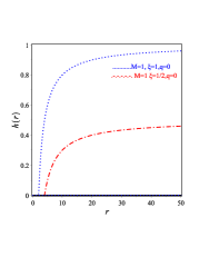
(a)  The metric potential of BH (9)

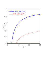
(b)  The metric potential of BH (18)

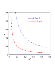
(c)  Hawking temperature of BH (9)

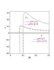
(d)  Hawking temperature of BH (18)

(e)  Entropy of BH (9)

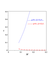
(f)  Entropy of BH (18)

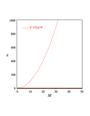
(g)  The energy of the BH (9)

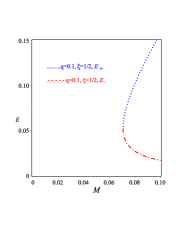
(h)  The energy of the BH (18)

Figure 1: Plot of the metric potential, Hawking temperature and the entropy of the BH (18).

and when $q=0$ we get $E=\frac{M(12\xi_{1}{}^{2}-\xi_{1}+2-12\xi_{1}{}^{3})}{12\xi^{2}(1-\xi_{1})}$ which is the quasi-local energy of the BH (9). The behavior of the quasi local energy for $q=0$ and $q\neq 0$ are drawn in Fig. 1 1(g) and 0(h) which also show positive increasing value for $E_{+}$ and decreasing value for $E_{-}$ when $\xi_{1}=1/2$ and $q\neq 0$.

V.2 Thermodynamics of the BHs (21) and (26)

Solution (26) is characterized by the BH mass $M$, the electric field $q$, the cosmological constant $\Lambda$ and the parameter $\xi_{4}$ and when the parameter $\xi_{4}=1$ we get the Reissner-Nordström (A)dS space-time. To find the horizons of this BH, (26), we put Eq. $h(r)=0$ which gives four roots two of them have real values and when $q=0$ we get one real positive root, i.e.,

$$r=\frac{2^{1/3}[(6M\sqrt{\Lambda}+\sqrt{2\xi_{4}{}^{3}+36M^{2}\Lambda})^{2/3}-\xi_{4}{}^{1/3}]}{2\sqrt{\Lambda}(6M\sqrt{\Lambda}+\sqrt{2\xi_{4}{}^{3}+36M^{2}\Lambda})^{1/3}}\,,$$ (36)

which is the horizon of the BH (21). The metric potentials of the BHs (21) and (26) are drawn in Fig. 2 1(a) and 1(b) respectively.

Using Eq. (29) we get the Hawking temperature whose form when $q=0$ gives

$$T=\frac{1}{4\pi}\Big{[}\frac{4M2^{1/3}\Lambda(6M\sqrt{\Lambda}+\sqrt{2\xi_{4}{}^{3}+36M^{2}\Lambda})^{2/3}}{[(6M\sqrt{\Lambda}+\sqrt{2\xi_{4}{}^{3}+36M^{2}\Lambda})^{2/3}-\xi_{4}{}^{1/3}]^{2}}+\frac{2\sqrt{\Lambda}2^{1/3}(6M\sqrt{\Lambda}+\sqrt{2\xi_{4}{}^{3}+36M^{2}\Lambda})^{2/3}-\xi_{4}{}^{1/3}]}{3(6M\sqrt{\Lambda}+\sqrt{2\xi_{4}{}^{3}+36M^{2}\Lambda})^{1/3}}\Big{]}\,.$$ (37)

The behavior of the Hawking temperature of the BHs (21) and (26) is drawn in Fig. 2 1(c) and 1(d) that show the behavior of the temperature for $\xi_{4}=1$ and $\xi_{4}=1/2$ and proves that $T_{+}>T_{-}$ for the BH (26). Using Eq. (30) we calculate the entropy and when $q=0$ we get the entropy of BH (21) whose behavior are figured out in Fig. 2 1(e) and 1(f). Using Eq. (31) we calculate the quasi-local energy of the BH (26) and when $q=0$ we get the quasi-local energy of the BH (21). The behavior of these energies are drawn in Fig. 2 1(g) for $q=0$ and in 2 0(h) for $q\neq 0$.

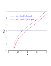
(a)  The metric potential of BH (21)

(b)  The metric potential of BH (26)

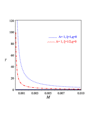
(c)  Hawking temperature of BH (21)

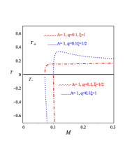
(d)  Hawking temperature of BH (26)

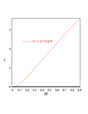
(e)  Entropy of BH (21)

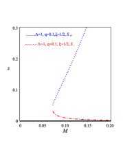
(f)  Entropy of BH (26)

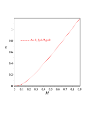
(g)  The energy (21)

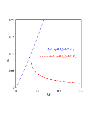
(h)  The energy (26)

Figure 2: Plot of the metric potential, Hawking temperature and the entropy of Eq. (26).

V.3 Fist law of thermodynamics

To test if the first law of thermodynamics of the BHs, (9), (18), (21) and (26) are satisfied or not we are going to use the formula given in $F(R)$ gravitational theory that has the form Zheng and Yang (2018b)

$$dE=TdS-Pdv,$$ (38)

where $E$, is the quasi-local energy defined by Eq. (31), $S$ is Bekenstein-Hawking entropy, $T$ is the Hawking temperature, $P$ is the radial component of the stress-energy tensor that plays the role of thermodynamical pressure, $P=T_{r}{}^{r}\mid_{\pm}$, and $V$ is the geometric volume of the space-time. The pressure, in the context of $F(R)$ gravitational theory, is defined as Zheng and Yang (2018b)

$$P=-\frac{1}{8\pi}\Big{\{}\frac{{\textit{F}_{R}}}{r_{\pm}{}^{2}}+\frac{1}{2}(f-R{\textit{F}_{R}})\Big{\}}+\frac{1}{4}\Big{(}\frac{2F}{r_{\pm}}+F^{\prime}\Big{)}T\,,$$ (39)

For the flat space-time given by Eq. (9) we get

$$P_{{}_{9}}=\frac{12M\xi r(1-\xi)-2r^{2}+r^{2}\xi+24M^{2}(\xi-1)+3Mr}{24rM(\xi-1)}=\frac{5\xi-4}{24\xi(\xi-1)}\,,$$ (40)

where we have substituted the value of $r$ from Eq. (32) in the case of $q=0$.

Using Eqs. (33) and (34) in case $q=0$ we get

$$T_{{}_{9}}dS_{{}_{9}}=\frac{8M(\xi-1)+r}{8r(\xi-1)}=\frac{4\xi^{2}-4\xi+1}{8(\xi-1)}.$$ (41)

Finally, using Eq. (35) in case $q=0$ we get

$$dE_{{}_{9}}=\frac{12M\xi(\xi-1)+2r-\xi r}{24M(\xi-1)}=\frac{6\xi^{2}(\xi-1)+2-\xi}{12\xi(\xi-1)}.$$ (42)

Using Eqs. (40), (41) and (42) we can easily show that the first law given by Eq. (38) is satisfied for the BH (9) when $\xi=1/2$. Using the same procedure for the BH (18) we get

$$P_{\pm(18)}=\frac{4q^{2}\xi_{1}{}^{2}+\xi_{1}(5M^{2}-2q^{2})+(\pm 5\xi_{1}M\mp 4M)\sqrt{M^{2}+q^{2}\xi_{1}}-4M^{2}}{24M(M\pm\sqrt{M^{2}+q^{2}\xi_{1}})(\xi_{1}-1)}\,,$$

$$T_{\pm(18)}dS_{\pm(18)}=\frac{[8M\xi_{1}(1-\xi_{1})+M\pm\sqrt{M^{2}+q^{2}\xi}][\xi_{1}q^{2}+M^{2}\pm M\sqrt{M^{2}+q^{2}\xi_{1}}]}{8M(M\pm\sqrt{M^{2}+q^{2}\xi_{1}})(\xi_{1}-1)}\,,$$

$$dE_{\pm(18)}=\frac{2M+(\pm 2\mp\xi_{1})\sqrt{M^{2}+q^{2}\xi_{1}}+\xi_{1}M(11-24\xi_{1}+12\xi_{1}{}^{2})}{24M\xi(\xi_{1}-1)}\,.$$ (43)

For the BH (21) we get

$$P_{(21)}=\frac{12M\xi_{2}(1-\xi_{2})-2r+r\xi_{2}+48r^{2}M\Lambda(\xi_{2}-1)+3M+6\Lambda r^{3}}{24M(\xi_{2}-1)}\,,$$

$$T_{(21)}dS_{(21)}=\frac{3M+2\Lambda r^{3}}{24M(\xi_{2}-1)}\,,\qquad dE_{(21)}=\frac{r(\xi_{2}-2+4\Lambda r^{2})}{24M\xi(\xi_{1}-1)}\,.$$ (44)

Substituting the value of $r$ from Eq. (36) and using Eq. (V.3) in (38) we can verify the 1st law of thermodynamics of the BH (21) when $\xi=1/2$. Finally, for the BH (26) we get

$$P_{(26)}=\frac{12Mr\xi_{4}(1-\xi_{4})-r^{2}(2-\xi_{4})-48r^{3}M\Lambda(1-\xi_{4})+2r^{4}\Lambda+3(Mr+q^{2})}{24Mr(\xi_{1}-1)}\,,$$

$$T_{(26)}dS_{(26)}=\frac{[8M(1-\xi_{4})+r][2\Lambda r^{4}-3(rM+q^{2})]}{24Mr^{2}(\xi_{1}-1)}\,,$$

$$dE_{(26)}=\frac{12M\xi_{4}(\xi_{4}-1)+r(2-\xi_{4})+48r^{2}M\Lambda(1-\xi_{4})-4r^{3}\Lambda}{24M(\xi_{1}-1)}\,.$$ (45)

Substituting the values of the positive roots of $h(r)$ given by Eq. (26) in (V.3) we can verify the first law of thermodynamics of the BH (26).

VI Summary of the main results

In this study, we have shown that for a spherically symmetric space-time that has equal metric potentials, i.e., $g_{tt}=\frac{1}{g_{rr}}$ there is only one solution that deviates from GR and asymptotes as a flat space-time for the specific class of ${\textit{F}(R)}$ that has the form ${\textit{F}(R)=R-2\alpha\sqrt{R}}$. Also for the space-time that asymptotes as (A)dS, there is also one BH that deviates from GR BH. To prove the preceding statements we apply the neutral field equation of ${\textit{F}(R)=R\pm F_{1}(R)}$ to a spherically symmetric space-time with metric potential has the form $h(r)=\xi-\frac{2M}{r}$ and shows that the only value that the parameter $\xi$ can take is $\xi=1/2$ to get a BH different from GR. We repeat the same technique for the charged case and reach the same conclusion. It is important to stress on the fact that some values for $\xi$, except 1/2, give ${\textit{F}_{1}(R)\propto R}$. The reason for this is the fact that any value of $\xi$ except than one makes Ricci scalar not vanishing, as is clear from Eq. (10), and the form of ${\textit{F}_{1}(R)}$ is always $\propto\frac{1}{r^{2}}$ which makes the form of ${\textit{F}(R)}$ always $\propto R.$ The only value that makes ${\textit{F}(R)\neq}R$ is $\xi=1/2$ because in that case ${\textit{F}_{1}(R)\propto\frac{1}{r}}$. The form of ${\textit{F}_{1}(R)}$ that makes the BHs different from GR has the form ${\textit{F}_{1}(R)=\mp\frac{\sqrt{R}}{3M}}$ and the Ricci scalar of these solution takes the form ${\textit{R}=\frac{1}{r^{2}}}$. We repeat the same calculations for a spherically symmetric space-time, with metric potential $h(r)=\xi-\frac{2M}{r}+\frac{2\Lambda r^{2}}{3}$, that asymptotes as (A)dS space-time and use the neutral and charged field equations of ${\textit{F}(R)}$ and proof that the only solution that deviates from GR exists only when $\xi=1/2$ and the form of ${\textit{F}_{1}(R)=\mp\frac{\sqrt{\textit{R}+8\Lambda}}{3M}}$. The Ricci scalar of this case takes the form ${\textit{R}}=\frac{1}{r^{2}}-8\Lambda$.

To make the picture more clear we calculate some thermodynamic quantities like entropy, Hawking temperature, quasi-local energy and Gibbs free energy for the two space-times that asymptotes as flat and (A)dS space-times. We show that for both space-times that the thermodynamic quantities for the parameter $\xi=1/2$ are physically acceptable consistent with the literature. Thus the case where $\xi=1/2$ that deviates from GR is physically acceptable from the viewpoint of thermodynamics. Finally, we showed by detail calculations that all the derived BHs, (9), (18), (21) and (26), satisfy the first law of thermodynamics given by Eq. (38).

It is well-known that for any null geodesic in the exterior region of the Schwarzschild metric the null geodesic equations are given by Claudel et al. (2001)

$$\frac{d^{2}r}{d\eta^{2}}=(r-3M)\Biggl{[}\left(\frac{d\theta}{d\eta}\right)^{2}+\sin^{2}\theta\left(\frac{d\phi}{d\eta}\right)^{2}\Biggr{]}\,,$$ (46)

where $\eta$ is the affine parameter along the geodesic. The R.H.S. of Eq. (46) has a positive value for $r>3M$ and has a negative value when $3M>r>2M$. For the BH (8), the null geodesic equations are given by

$$\frac{d^{2}r}{d\eta^{2}}=\frac{1}{2}(r-6M)\Biggl{[}\left(\frac{d\theta}{d\eta}\right)^{2}+\sin^{2}\theta\left(\frac{d\phi}{d\eta}\right)^{2}\Biggr{]}\,.$$ (47)

The R.H.S. of Eq. (47) has a positive value when $r>6M$ and negative value when $6M>r>4M$. Therefore, for any future endless null geodesic in the maximally extended space-time given by Eq. (8) starting at some point with $6M<r$ and initially directed outwards, in the sense that $\frac{dr}{d\eta}$ is initially positive, will continue outwards and escape to infinity. Any future endless null geodesic in the maximally extended space-time given by Eq. (8) starting at some point with $r:6M>r>4M$ and initially directed inwards, in the sense that $\frac{dr}{d\eta}$ is initially negative will continue inwards and fall into the black hole. The hypersurface ${r=6M}$, known as the photon sphere of the space-time (8), thus distinguishes the borderline between these two types of behavior; any null geodesic starting at some point of the photon sphere and initially tangent to the photon sphere will remain in the photon sphere; for more detail, see Darwin (1961, 1959).

To conclude, we have shown that in the frame of ${\textit{F}(R)=R+F_{1}(R)}$ there is only a unique spherically symmetric BH, form the line-element which has equal metric potential, that is different from GR which asymptotes as flat or (A)dS space-times. Is this result valid for the spherically symmetric line-element that has unequal metric potentials? If yes is its thermodynamic quantities are acceptable? These questions will be answered elsewhere.

References

- Stelle (1977) K. S. Stelle, Phys. Rev. D 16, 953 (1977).
- Nojiri and Odintsov (2006) S. Nojiri and S. D. Odintsov, eConf C0602061, 06 (2006), [Int. J. Geom. Meth. Mod. Phys.4,115(2007)], arXiv:hep-th/0601213 [hep-th] .
- Copeland et al. (2006) E. J. Copeland, M. Sami, and S. Tsujikawa, Int. J. Mod. Phys. D15, 1753 (2006), arXiv:hep-th/0603057 [hep-th] .
- Nojiri and Odintsov (2011) S. Nojiri and S. D. Odintsov, Phys. Rept. 505, 59 (2011), arXiv:1011.0544 [gr-qc] .
- Awad et al. (2018a) A. Awad, W. El Hanafy, G. Nashed, S. Odintsov, and V. Oikonomou, JCAP 07, 026 (2018a), arXiv:1710.00682 [gr-qc] .
- Clifton et al. (2012) T. Clifton, P. G. Ferreira, A. Padilla, and C. Skordis, Phys. Rept. 513, 1 (2012), arXiv:1106.2476 [astro-ph.CO] .
- Tang et al. (2019) Z.-Y. Tang, B. Wang, and E. Papantonopoulos, (2019), arXiv:1911.06988 [gr-qc] .
- Awad et al. (2018b) A. Awad, W. El Hanafy, G. Nashed, and E. N. Saridakis, JCAP 02, 052 (2018b), arXiv:1710.10194 [gr-qc] .
- Podolsky et al. (2018) J. Podolsky, R. Svarc, V. Pravda, and A. Pravdova, Phys. Rev. D98, 021502 (2018), arXiv:1806.08209 [gr-qc] .
- Lü et al. (2015) H. Lü, A. Perkins, C. N. Pope, and K. S. Stelle, Phys. Rev. D92, 124019 (2015), arXiv:1508.00010 [hep-th] .
- Bueno and Cano (2017) P. Bueno and P. A. Cano, Class. Quant. Grav. 34, 175008 (2017), arXiv:1703.04625 [hep-th] .
- Bueno and Cano (2016) P. Bueno and P. A. Cano, Phys. Rev. D94, 124051 (2016), arXiv:1610.08019 [hep-th] .
- De Felice and Tsujikawa (2010) A. De Felice and S. Tsujikawa, Living Rev. Rel. 13, 3 (2010), arXiv:1002.4928 [gr-qc] .
- Cognola et al. (2008) G. Cognola, E. Elizalde, S. Nojiri, S. D. Odintsov, L. Sebastiani, and S. Zerbini, Phys. Rev. D77, 046009 (2008), arXiv:0712.4017 [hep-th] .
- Pogosian and Silvestri (2008) L. Pogosian and A. Silvestri, Phys. Rev. D 77, 023503 (2008).
- Pogosian and Silvestri (2010) L. Pogosian and A. Silvestri, Phys. Rev. D 81, 049901 (2010).
- Zhang (2006) P. Zhang, Phys. Rev. D73, 123504 (2006), arXiv:astro-ph/0511218 [astro-ph] .
- Li and Barrow (2007) B. Li and J. D. Barrow, Phys. Rev. D75, 084010 (2007), arXiv:gr-qc/0701111 [gr-qc] .
- Song et al. (2007) Y.-S. Song, H. Peiris, and W. Hu, Phys. Rev. D76, 063517 (2007), arXiv:0706.2399 [astro-ph] .
- Nojiri and Odintsov (2008) S. Nojiri and S. D. Odintsov, Phys. Rev. D77, 026007 (2008), arXiv:0710.1738 [hep-th] .
- Nojiri and Odintsov (2007) S. Nojiri and S. D. Odintsov, Phys. Lett. B657, 238 (2007), arXiv:0707.1941 [hep-th] .
- Capozziello et al. (2018) S. Capozziello, C. A. Mantica, and L. G. Molinari, Int. J. Geom. Meth. Mod. Phys. 16, 1950008 (2018), arXiv:1810.03204 [gr-qc] .
- Vainio and Vilja (2017) J. Vainio and I. Vilja, Gen. Rel. Grav. 49, 99 (2017), arXiv:1603.09551 [astro-ph.CO] .
- Ostrogradsky (1850) M. Ostrogradsky, Mem. Acad. St. Petersbourg 6, 385 (1850).
- Woodard (2007) R. P. Woodard, The invisible universe: Dark matter and dark energy. Proceedings, 3rd Aegean School, Karfas, Greece, September 26-October 1, 2005, Lect. Notes Phys. 720, 403 (2007), arXiv:astro-ph/0601672 [astro-ph] .
- Starobinsky (1980) A. A. Starobinsky, Phys. Lett. B91, 99 (1980), [,771(1980)].
- Carroll et al. (2003) S. M. Carroll, M. Hoffman, and M. Trodden, Phys. Rev. D68, 023509 (2003), arXiv:astro-ph/0301273 [astro-ph] .
- Carroll et al. (2004) S. M. Carroll, V. Duvvuri, M. Trodden, and M. S. Turner, Phys. Rev. D70, 043528 (2004), arXiv:astro-ph/0306438 [astro-ph] .
- Capozziello (2002) S. Capozziello, Int. J. Mod. Phys. D11, 483 (2002), arXiv:gr-qc/0201033 [gr-qc] .
- Capozziello et al. (2003) S. Capozziello, V. F. Cardone, S. Carloni, and A. Troisi, Int. J. Mod. Phys. D12, 1969 (2003), arXiv:astro-ph/0307018 [astro-ph] .
- Multamaki and Vilja (2006) T. Multamaki and I. Vilja, Phys. Rev. D74, 064022 (2006), arXiv:astro-ph/0606373 [astro-ph] .
- Nashed (2018a) G. G. L. Nashed, European Physical Journal Plus 133, 18 (2018a).
- Multamaki and Vilja (2007) T. Multamaki and I. Vilja, Phys. Rev. D76, 064021 (2007), arXiv:astro-ph/0612775 [astro-ph] .
- de la Cruz-Dombriz et al. (2009) A. de la Cruz-Dombriz, A. Dobado, and A. L. Maroto, Phys. Rev. D80, 124011 (2009), [Erratum: Phys. Rev.D83,029903(2011)], arXiv:0907.3872 [gr-qc] .
- Nashed (2018b) G. G. L. Nashed, International Journal of Modern Physics D 27, 1850074 (2018b).
- Hendi et al. (2012) S. H. Hendi, B. Eslam Panah, and S. M. Mousavi, Gen. Rel. Grav. 44, 835 (2012), arXiv:1102.0089 [hep-th] .
- Nashed (2018) G. G. L. Nashed, Adv. High Energy Phys. 2018, 7323574 (2018).
- Sebastiani and Zerbini (2011) L. Sebastiani and S. Zerbini, Eur. Phys. J. C71, 1591 (2011), arXiv:1012.5230 [gr-qc] .
- Nashed and Capozziello (2019) G. G. L. Nashed and S. Capozziello, Phys. Rev. D99, 104018 (2019), arXiv:1902.06783 [gr-qc] .
- Elizalde et al. (2020) E. Elizalde, G. G. L. Nashed, S. Nojiri, and S. D. Odintsov, Eur. Phys. J. C80, 109 (2020), arXiv:2001.11357 [gr-qc] .
- Nashed et al. (2020) G. Nashed, W. El Hanafy, S. Odintsov, and V. Oikonomou, Int. J. Mod. Phys. D 29, 2050090 (2020), arXiv:1912.03897 [gr-qc] .
- Akiyama et al. (2019) K. Akiyama et al. (Event Horizon Telescope), Astrophys. J. 875, L1 (2019), arXiv:1906.11238 [astro-ph.GA] .
- Falcke et al. (2000) H. Falcke, F. Melia, and E. Agol, Astrophys. J. Lett. 528, L13 (2000), arXiv:astro-ph/9912263 .
- Buchdahl (1970) H. A. Buchdahl, mnras 150, 1 (1970).
- Nojiri and Odintsov (2003) S. Nojiri and S. D. Odintsov, Phys. Rev. , 123512 (2003), arXiv:hep-th/0307288 [hep-th] .
- Capozziello and De Laurentis (2011) S. Capozziello and M. De Laurentis, Phys. Rept. 509, 167 (2011), arXiv:1108.6266 [gr-qc] .
- Nojiri et al. (2017) S. Nojiri, S. D. Odintsov, and V. K. Oikonomou, Phys. Rept. 692, 1 (2017), arXiv:1705.11098 [gr-qc] .
- Cognola et al. (2005) G. Cognola, E. Elizalde, S. Nojiri, S. D. Odintsov, and S. Zerbini, jcap 2, 010 (2005), hep-th/0501096 .
- Schwarzschild (1916) K. Schwarzschild, Abh. Konigl. Preuss. Akad. Wissenschaften Jahre 1906,92, Berlin,1907 1916, 189 (1916).
- Reissner (1916) H. Reissner, Annalen der Physik 355, 106 (1916).
- Sheykhi (2012) A. Sheykhi, Phys. Rev. D 86, 024013 (2012).
- Sheykhi (2010) A. Sheykhi, Eur. Phys. J. C69, 265 (2010), arXiv:1012.0383 [hep-th] .
- Hendi et al. (2010) S. H. Hendi, A. Sheykhi, and M. H. Dehghani, Eur. Phys. J. C70, 703 (2010), arXiv:1002.0202 [hep-th] .
- Sheykhi et al. (2010) A. Sheykhi, M. H. Dehghani, and S. H. Hendi, Phys. Rev. D 81, 084040 (2010).
- Cognola et al. (2011) G. Cognola, O. Gorbunova, L. Sebastiani, and S. Zerbini, Phys. Rev. D 84, 023515 (2011).
- Zheng and Yang (2018a) Y. Zheng and R.-J. Yang, Eur. Phys. J. C78, 682 (2018a), arXiv:1806.09858 [gr-qc] .
- Zheng and Yang (2018b) Y. Zheng and R. Yang, The European Physical Journal C 78 (2018b), 10.1140/epjc/s10052-018-6167-4.
- Claudel et al. (2001) C.-M. Claudel, K. Virbhadra, and G. Ellis, J. Math. Phys. 42, 818 (2001), arXiv:gr-qc/0005050 .
- Darwin (1961) C. G. Darwin, Proceedings of the Royal Society of London. Series A. Mathematical and Physical Sciences 263, 39 (1961), https://royalsocietypublishing.org/doi/pdf/10.1098/rspa.1961.0142 .
- Darwin (1959) C. G. Darwin, Proceedings of the Royal Society of London. Series A. Mathematical and Physical Sciences 249, 180 (1959), https://royalsocietypublishing.org/doi/pdf/10.1098/rspa.1959.0015 .