The hydrogen atom:
consideration of the electron self-field

Keywords: Spinor electrodynamics. Dirac-Maxwell system of equations. Solitonlike solutions. Spectrum of characteristics. “Bohrian” law for binding energies

PACS: 03.50.-z; 03.65.-w; 03.65.-Pm

1 THE HYDROGEN ATOM AND CLASSICAL FIELD MODELS OF ELEMENTARY PARTICLES

It is well known that the successful description of the hydrogen atom, first in Bohr’s theory, and then via solutions to the Schrödinger equation was one of the main motivations for the development of quantum theory. Later, Dirac described almost perfectly the observed hydrogen spectrum using his relativistic generalization of the Schrödinger equation. A slight deviation from experiment (the Lamb shift between $2s_{1/2}$ and $2p_{1/2}$ levels in the hydrogen atom) discovered later was interpreted as the effect of electron interaction with vacuum fluctuations of electromagnetic field and explained in the framework of quantum electrodynamics (QED) using second quantization.

Nonetheless, the problem of the description of the hydrogen atom still attracts attention of researchers, and, in some sense, is a ‘‘touchstone’’ for many new theoretical developments. In particular, it is possible to obtain the energy spectrum via purely algebraic methods  [1]. Theories of the ’’supersymmetric’’ hydrogen atom are also widespread [2]. In the framework of the classical ideas, the spectrum can be explained by the absence of radiation for the electron motion along certain “stable” orbits. This effect can be related with the balance of radiation and absorption of energy from a hypothetical random electromagnetic background in the framework of stochastic electrodynamics [3], or it takes place in soliton models of the hydrogen atom [4].

The difficulties related to the description of the hydrogen atom in canonical relativistic quantum mechanics and quantum electrodynamics (QED) include the “strange” singularity $\sim r^{-\alpha},\leavevmode\nobreak\ \alpha=e^{2}/\hbar c\approx 0.007$ of the Dirac wave function at zero for s- and p- states which appears in spite of the initial requirement of solution regularity. Consideration of the magnetic field of the proton via perturbation theory alone does not seem quite correct since the magnetic potential near zero is of the order $1/r^{2}$ and dominates over the Coulomb potential. This problem was discussed, in particular, in  [5] (see also [6]), where the possibility of constructing a magnetic theory of nuclear forces was considered.

Of special topicality is consideration of the electromagnetic self-field of the electron. From the point of view of quantum ideas, the electron in the hydrogen atom represents a spatially distributed system according to the probability density $\Psi^{+}\Psi$ whose elements interact both with the field of the nucleus and between each other. Since the absolute value of the electron charge is equal to the proton charge, the proton field turns out to be screened at large distances.

It is known that consideration of the self-consistent collective field of electrons is necessary for multielectron atoms, and is phenomenologically implemented, for example, in the Hartree–Fock method. The multielectron wave function, however, does not differ fundamentally from the single-electron function. Consideration of the self-action of the spatially distributed electron charge density does not contradict the ideas of its “point-like” character (see discussion in [7, 8]).

Note also that a similar effect of gravitational selfaction of a “free” quantum particle was proposed in [9, 10, 11] and other works in the context of the hypothesis on the objective character of the process of reduction of the particle wave function.

It should be noted that the problem of consideration of the electron self-field (self-energy) and its effect on the observed energy levels is one of the central problems in the context of QED (see, e.g., [12]). According to the most widely accepted ideas, the effect is related to interaction of the electron with the second quantized electromagnetic field of “vacuum fluctuations”  [13].The calculation of its value via perturbation theory (see, e.g.,  [14]) results in infinite shifts of energy levels which, after mass renormalization, are reduced to the values of radiative corrections (Lamb shift etc.) that agree well with experiment.

There were attempts to reproduce all the basic results of QED without second quantization. Thus, the approach used by Barut [15, 16, 17] is based on the analysis of the self-consistent Dirac-Maxwell system of equations studied in this paper, and, essentially, it is purely classical. Nonetheless, the perturbation theory and a simple regularization procedure ensure exact reproduction of all radiative corrections usually calculated in the QED formalism.

The effect of the self-field of the electron, as noted above, is “nonperturbative” and is not reduced to radiative corrections. Consideration of this effect completely alters the mathematical structure of the model, making it essentially nonlinear. It can be assumed that the divergences in Barut’s approach (and correspondingly, QED) could arise due to the absence of an exact solution to the initial classical Dirac-Maxwell system which might serve as the initial approximation in the applied perturbation theory [18].

Thus, we naturally arrive at examination of regular solutions to the self-consistent effective nonlinear system of coupled Dirac and Maxwell equations (in the presence of the additional external Coulomb field of the proton). Note that such systems of equations were considered earlier in the context of construction of an interesting class of classical soliton models of elementary particles.

Such models are based on the well proven linear field equations of Schrödinger, Klein–Gordon, Dirac, and Maxwell . In this case, the effective nonlinearity appears only as a consequence of interaction between different fields, and the form of this interaction is well defined by the requirement of gauge invariance.

The founder of this approach is, perhaps, N. Rosen, who considered stationary spherically symmetric so-called particle-like (i.e., everywhere regular with finite Noether’s integrals of motion) solutions to the Klein-Gordon and Maxwell system of equations with minimal electromagnetic interaction between them in [19].

Later, this approach was extended to the (mathematically much more complicated) system of Dirac-Maxwell equations with minimal electromagnetic interaction between fields [20, 21, 22, 23]. It is especially interesting that this system is a classical analog of operator equations of quantum electrodynamics. It was shown, in particular, that charged fermions with any half-integer spin can be described in a unified way in the framework of this model [21, 24].

Note now that the real particles’ properties are directly manifested if only they move in external, in particular, electromagnetic, fields. Examination of the corresponding nonstationary particle-like solutions is quite complicated. In this regard, stationary solutions to the Dirac-Maxwell system of equations in the presence of an external Coulomb potential turn out to be physically attractive and mathematically feasible for consideration.

For hydrogen-like atoms regular solutions to a nonrelativistic analog of the considered system, the self-consistent system of Schrödinger–Poisson equations, were considered in [18]; however, just for the case of “pure” hydrogen ($Z=1$) a solution had not been found. Preliminary examination and search for particle-like (or, using modern terminology, soliton-like) solutions in the relativistic Dirac-Maxwell model of the hydrogen atom can be found in [25] (see also [26]). In this paper, we specify more precisely and develop the results of these previous studies.

2 FIELD EQUATIONS AND BASIC PARAMETERS OF SOLUTIONS

We consider the self-consistent system of Dirac-Maxwell equations in Minkowski space $\bf M$ with the metric $\eta_{\mu\nu}=diag\{+1,-1,-1,-1\}$ and coordinates $\{X^{\mu}\},\leavevmode\nobreak\ \mu=0,1,2,3$. This system of equations corresponds to the Lagrangian of the form

$$L=-\frac{1}{16\pi}F^{2}+\frac{\hbar c}{2}\{i\bar{\Psi}\gamma^{\mu}\partial_{\mu}\Psi-i\partial_{\mu}\bar{\Psi}\gamma^{\mu}\Psi-2k\bar{\Psi}\Psi\}+eA_{\mu}\bar{\Psi}\gamma^{\mu}\Psi.$$ (1)

Here, $\partial_{\mu}:=\partial/\partial X^{\mu}$,  $\{\gamma^{\mu}\}$ are the $4\times 4$ Dirac matrices in the canonical representation, $\Psi$ is the Dirac bispinor, $\bar{\Psi}:=\Psi^{+}\gamma^{0}$, $\{A_{\mu}\}$ are the 4-potentials of electromagnetic (EM) field, and $F^{2}=F_{\mu\nu}F^{\mu\nu}$ is the main invariant expressed in terms of EM field strength tensor $F_{\mu\nu}=\partial_{\mu}A_{\nu}-\partial_{\nu}A_{\mu}$.

It is assumed that the scalar potential $A_{0}$ includes, along with the regular part, the fixed singular part $A_{0}^{ex}=e/R$, where $e$ is the elementary charge. This part corresponds to the external Coulomb field of the proton.

The quantities $\hbar,k$, generally speaking, represent some scaling coefficients whose numerical values should be found from the comparison of the parameters of some standard solution (corresponding, for example, to the ground state of the hydrogen atom) with experimental values. However, it should be expected from the agreement with the quantum theory that these quantities correspond to the canonical constants, the Planck constant ($\hbar=h/2\pi$) and the inverse Compton electron length $k=mc/\hbar$, where $m$ is the electron mass.

By varying the action $S=\int Ld^{4}x$ over $\bar{\Psi}$ and $A_{\mu}$ and applying the Lorentz gauge condition $\partial_{\mu}A^{\mu}=0$ to the potentials, we obtain the field equations of the form

$$i\gamma^{\mu}(\partial_{\mu}-i(e/\hbar c)(A_{\mu}+A_{\mu}^{ex})\Psi-k\Psi=0,\leavevmode\nobreak\ \leavevmode\nobreak\ \Box A^{\mu}=4\pi e\bar{\Psi}\gamma^{\mu}\Psi,$$ (2)

where $A_{\mu}^{ex}=\{e/R,0,0,0\}$.

Now, we impose on the sought solutions of system (2) the condition of electroneutrality $|Q|=e$, i.e., the condition of equality of the absolute value of the electron distribution charge $Q=-e\int\Psi^{+}\Psi d^{3}X$ and the proton charge $e$. Satisfaction of this condition is equivalent to the following:

$$\int\Psi^{+}\Psi d^{3}X=1,$$ (3)

so that it automatically guarantees normalization of the “wave function” of electron distribution, although originally the field $\Psi$ can be considered classical .

Using scale transformations of coordinates (converting lengths to the Compton scale) and field functions of the form

$$X_{\mu}\mapsto x_{\mu}/k,\leavevmode\nobreak\ A_{\mu}\mapsto\frac{ke}{\alpha}a_{\mu},\leavevmode\nobreak\ \Psi\mapsto\left(\frac{k^{3}}{4\pi\alpha}\right)^{1/2}\psi,$$ (4)

we obtain the Lagrangian

$$l=-\frac{1}{16\pi}f^{2}+\frac{1}{8\pi}\{i\bar{\psi}\gamma^{\mu}\partial_{\mu}\psi-i\partial_{\mu}\bar{\psi}\gamma^{\mu}\psi-2\bar{\psi}\psi+2(a_{\mu}+a_{\mu}^{ex})\bar{\psi}\gamma^{\mu}\psi\},\leavevmode\nobreak\ \leavevmode\nobreak\ a_{\mu}^{ex}=\{\frac{\alpha}{r},0,0,0\},$$ (5)

and the corresponding field equations

$$i\gamma^{\mu}(\partial_{\mu}-i(a_{\mu}+a_{\mu}^{ex}))\psi-\psi=0,\leavevmode\nobreak\ \leavevmode\nobreak\ \Box a^{\mu}=\bar{\psi}\gamma^{\mu}\psi,$$ (6)

which do not contain any dimensional parameters. The only dimensionless parameter, the fine structure constant $\alpha:=e^{2}/\hbar c\approx 1/137$, enters only the expression for the Coulomb potential $a_{0}^{ex}=\alpha/r$ and the condition of electroneutrality/normalization which takes the following form in terms of dimensionless variables:

$$\frac{1}{4\pi}\int\psi^{+}\psi d^{3}x=\alpha.$$ (7)

Note that dimensional parameters corresponding to original Lagrangian (1) are connected with the corresponding dimensionless quantities extracted from (5) and given in Section 4 as follows:

• For the Lagrangian

  $$L=\frac{\hbar ck^{4}}{\alpha}l;$$ (8)

• for the energy

  $$W=\frac{\hbar ck}{\alpha}w\equiv\frac{mc^{2}}{\alpha}w;$$ (9)

• for the total angular momentum vector

  $${\bf J}=\frac{\hbar}{\alpha}{\bf j};$$ (10)

• for electric charge (if (7) is satisfied)

  $$Q=-e;$$ (11)

• and for the magnetic moment vector

  $${\bf M}=\frac{e}{k\alpha}{\bf m}\equiv\frac{1}{\alpha}\left(\frac{e\hbar}{mc}\right){\bf m}.$$ (12)

Hereinafter, our basic task is to obtain regular solutions to system of equations (6) with Lorentz gauge and electroneutrality condition (7); we consider only stationary solutions of the form

$$\psi^{T}=\{\kappa^{T}({\bf r}),\leavevmode\nobreak\ \chi^{T}({\bf r})\}e^{-i\omega t},\leavevmode\nobreak\ \leavevmode\nobreak\ a_{\mu}=\{\phi({\bf r}),\bf a({\bf r})\},$$ (13)

where $\kappa,\chi$ are the 2-spinors, $\phi,\bf a$ are the scalar and vector electromagnetic potentials, respectively, and the symbol ‘T’ denotes transposition.

3 $\alpha$-EXPANSION
AND THE NONRELATIVISTIC LIMIT $\alpha\rightarrow 0$

In stationary case (13) the basic system of equations (6) takes the form

$$\begin{array}[]{l}{\bf\Sigma}\cdot(i\nabla-{\bf a})\chi=(\omega+\phi+\alpha/r-1)\kappa,\\ {\bf\Sigma}\cdot(i\nabla-{\bf a})\kappa=(\omega+\phi+\alpha/r+1)\chi,\\ \Delta\phi=\kappa^{+}\kappa+\chi^{+}\chi,\\ \Delta{\bf a}=\kappa^{+}{\bf\Sigma}\chi+\chi^{+}{\bf\Sigma}\kappa,\end{array}$$ (14)

with the electroneutrality condition $(4\pi)^{-1}\int(\kappa^{+}\kappa+\chi^{+}\chi)d^{3}x=\alpha$. Here ${\bf\Sigma}=\{{\bf\Sigma}_{a}\},a=1,2,3$ is the set of Pauli matrices in the standard representation.

Let us now make one more transformation of coordinates and field functions [25], to convert length to the Bohrian scale and expand the solutions over the small parameter $\alpha$. Namely, let us introduce the new coordinates $\bf X$, 2-spinors $K,N$ and the potentials $\Phi,\bf A$ (not to be confused with the original dimensional ones) as follows:

$$\begin{array}[]{l}{\bf x}={\bf X}/(\alpha(1+\omega)),\\ \kappa=\alpha^{2}(1+\omega)^{3/2}K,\leavevmode\nobreak\ \leavevmode\nobreak\ \chi=\alpha^{3}(1+\omega)^{3/2}N,\\ \phi=\alpha^{2}(1+\omega)\Phi,\leavevmode\nobreak\ \leavevmode\nobreak\ {\bf a}=\alpha^{3}(1+\omega)\bf A.\end{array}$$ (15)

Then system (14) takes the form

$$\begin{array}[]{l}{\bf\Sigma}\cdot(i\nabla-\alpha^{2}{\bf A})N=(-\varepsilon+\Phi+1/R)K,\\ {\bf\Sigma}\cdot(i\nabla-\alpha^{2}{\bf A})K=(1+\alpha^{2}(\Phi+1/R))N,\\ \Delta\Phi=K^{+}K+\alpha^{2}N^{+}N,\\ \end{array}$$ (16)

while the additional equation for the magnetic potential reads

$$\Delta{\bf A}=K^{+}{\bf\Sigma}N+N^{+}{\bf\Sigma}K,$$ (17)

and the electroneutrality condition takes the form $(4\pi)^{-1}\int(K^{+}K+\alpha^{2}N^{+}N)d^{3}X=1$. Here, the “reduced frequency” is

$$\varepsilon:=(1-\omega)/(\alpha^{2}(1+\omega)),$$ (18)

and it follows from the analysis of the asymptotics (see below) that solutions (16) decreasing at infinity can exist only for $|\omega|<1$, , so the parameter $\varepsilon$ is always positive.

The new form of Eqs. (16) is convenient because, due to the smallness of the parameter $\alpha$, the “zero” approximation $\alpha\rightarrow 0$ can be considered in a consistent way. Indeed, by discarding terms $\sim\alpha^{2}$, we obtain for the first three Eqs. (16) and the electroneutrality condition

$$\begin{array}[]{l}i{\bf\Sigma}\cdot\nabla K=N,\\ i{\bf\Sigma}\cdot\nabla N=(-\varepsilon+\Phi+1/R)K,\\ \Delta\Phi=K^{+}K,\\ (4\pi)^{-1}\int K^{+}Kd^{3}X=1,\end{array}$$ (19)

System (19) is closed, it contains the only parameter $\varepsilon$ to be defined, and it does not include terms with the magnetic potential. The latter can be defined from the prefound solutions to limiting system (19) by integration of Eq (17). In this case, system (19) after substituting the expression for the 2-spinor $N$ from the first equation to the second equation is reduced to one second order equation for the main 2-spinor $K$. After simple transformations, we obtain the following final form of the system in the leading approximation with respect to $\alpha$:

$$\begin{array}[]{l}\Delta K=(\varepsilon-\Phi-1/R)K,\\ \Delta\Phi=K^{+}K,\\ (4\pi)^{-1}\int K^{+}Kd^{3}X=1.\end{array}$$ (20)

The structure of system (20) is close (but not identical) to the self-consistent system of Schrödinger– Newton equations which attracted attention earlier thanks to the ideas of Diosi [9], Penrose [10] and others, on the possible self-gravitating nature of reduction of the particle wave function mentioned above. In particular, the spectrum of stationary spherically symmetric regular solutions to the Schrödinger–Newton system was numerically obtained in [28, 11].

The Schrödinger-Newton system differs from system (20) by the absence of an external Coulomb (Newtonian) potential and the sign of potential in the first equation of type (20) (which is connected with the different signs of the gravitational and electrostatic interactions). It can be easily seen that in reality (20) represents a self-consistent system of Schrödinger-Poisson equations (written for the case of stationary solutions), so that the transition to the limit $\alpha\mapsto 0$ and system (19) or (20) represent, in essence, the nonrelativistic approximation of the original Dirac-Maxwell system.

Regular solutions the Schrödinger-Poisson equations are in fact the main subject of the study below. As for the problem of finding relativistic corrections, it is quite complicated, since, as will be shown later, in the general case it results in an infinite chain of equations for radial functions.

It should be noted that systems of equations similar to (20) were proposed more than once as a physically justified alternative to the linear Schrödinger equation. Schrödinger himself discussed the need to consider the “spatial distribution” of the electron charge, including the case of multielectron atoms [27, p. 116], and the possibility of introducing a “neutralization potential” for this purpose [27, p. 175], i.e., the potential of the self-field of electrons. Detailed examination of these issues can be found in [7].

To the best of our knowledge, the first attempts to obtain the regular solutions to system (20) and the corresponding binding energies were made in  [25] and  [18]. In  [18] these solutions were found for lowest s-states (with $n=1,2,3$) for different nuclear charge $Ze$ of hydrogen-like atoms; the iteration method was used, and wave functions of the canonical linear quantum mechanical problem were taken as the first approximation.

The obtained energy level shifts, as expected, turned out large, and in order to agree with the observed values, it was proposed to use an analog of renormalization. However, the correctness of the procedure of finding solutions raises doubts . Anyway, the shift was not determined for the most important case of hydrogen itself ($Z=1$).

A more reliable method of the numerical solution for system (20), together with the variational method (in the class of the same trial functions as in the linear quantum mechanical problem), was used in ([25, 26]). Moreover, the solutions found therein can be used to find the magnetic potential and the electron angular momentum in different states of the hydrogen atom by integrating Eq. (17).

4 AXIALLY SYMMETRIC SOLUTIONS: SEPARATION OF ANGULAR DEPENDENCE AND THE PROBLEM OF ENTANGLEMENT OF HARMONICS

Strictly speaking, the system of equations (19) under study has no spherically symmetric solutions due to the spinor nature of the functions $K,N$ and the presence of magnetic potential of the electron field calculated from additional Eq. (17). System (20) itself, however, can be reduced to an equation for one spherical harmonic corresponding to the main 2-spinor $K$ and the corresponding potential $\Phi$. Indeed, by assuming the potential spherically symmetric, it can be seen that the angular dependence in the equations for the spinor functions in (19) can be described by any pair of corresponding spherical spinors, i.e., similarly to the linear problem of quantum mechanics. On the other hand, the corresponding electric charge density $\sim K^{+}K$ in the right-hand part of (19) is not necessarily spherically symmetric, so the system turns out to be unclosed and requires additional harmonics of the potential (corresponding to the quadrupole and higher even moments). The inevitable appearance of these harmonics, in turn, requires introduction of the corresponding pairs of higher order spherical spinors, and so on. This situation results in the requirement to consider an infinite chain of equations for radial functions, and it is difficult to substantiate the cut in this chain because of the absence of any small parameter. This problem was considered in detail in [24].

The only possibility to obtain a closed system of equations is the choice of such initial pairs of spherical spinors for which the corresponding electric charge density is spherically symmetric (below, we denote the radial variable $R\mapsto r$ for simplicity)

Thus, the choice of the angular dependence of the field functions is limited by the following two possibilities corresponding, from the point of view of canonical quantum mechanics, to s- and p-states with the eigenvalues of the operator of orbital angular momentum $l=0,1$ respectively:

ansatz А:

$$\Phi=\phi(r),\leavevmode\nobreak\ \leavevmode\nobreak\ K=k(r)\left(\begin{array}[]{l}1\\ 0\end{array}\right),\leavevmode\nobreak\ \leavevmode\nobreak\ N=in(r)\left(\begin{array}[]{l}\cos{\theta}\\ \sin{\theta}\ e^{i\varphi}\end{array}\right),$$ (21)

while, after the replacement $K\leftrightarrow N$, we have ansatz B:

$$\Phi=\phi(r),\leavevmode\nobreak\ \leavevmode\nobreak\ K=ik(r)\left(\begin{array}[]{l}\cos{\theta}\\ \sin{\theta}\ e^{i\varphi}\end{array}\right),\leavevmode\nobreak\ \leavevmode\nobreak\ N=n(r)\left(\begin{array}[]{l}1\\ 0\end{array}\right).$$ (22)

Note that two more substitutions are possible, along with the two angular dependences given above:

$$\Phi=\phi(r),\leavevmode\nobreak\ \leavevmode\nobreak\ K=k(r)\left(\begin{array}[]{l}0\\ 1\end{array}\right),\leavevmode\nobreak\ \leavevmode\nobreak\ N=in(r)\left(\begin{array}[]{l}-\sin{\theta}\ e^{-i\varphi}\\ \leavevmode\nobreak\ \leavevmode\nobreak\ \leavevmode\nobreak\ \cos{\theta}\end{array}\right),$$ (23)

or

$$\Phi=\phi(r),\leavevmode\nobreak\ \leavevmode\nobreak\ K=ik(r)\left(\begin{array}[]{l}-\sin{\theta}\ e^{-i\varphi}\\ \leavevmode\nobreak\ \leavevmode\nobreak\ \leavevmode\nobreak\ \cos{\theta}\end{array}\right),\leavevmode\nobreak\ \leavevmode\nobreak\ N=n(r)\left(\begin{array}[]{l}0\\ 1\end{array}\right),$$ (24)

conjugate to the ansatzes $\bf A$ and $\bf B$  respectively. It can be easily verified that they result in the same form of system (20), and the corresponding solutions differ only by the signs of projections of the magnetic moment and the total angular momentum. Therefore, we will not consider them separately. For both substitutions $\bf A$ and $\bf B$ main system of equations (19) and system (20) following from it turn out consistent and closed. Namely, for $\bf A$ we obtain:

$$\begin{array}[]{l}k^{\prime}=n,\leavevmode\nobreak\ \leavevmode\nobreak\ n^{\prime}+(2/r)n=(\varepsilon-\phi-(1/r))k\\ \mapsto k^{\prime\prime}+(2/r)k^{\prime}=(\varepsilon-\phi-(1/r))k,\\ \phi^{\prime\prime}+(2/r)\phi^{\prime}=k^{2},\\ \int k^{2}r^{2}dr=1,\\ \lambda^{\prime\prime}+(2/r)\lambda^{\prime}-(2/r^{2})\lambda=2kk^{\prime},\end{array}$$ (25)

and for $\bf B$ we obtain:

$$\begin{array}[]{l}k^{\prime}+(2/r)k=-n,\leavevmode\nobreak\ \leavevmode\nobreak\ n^{\prime}=-(\varepsilon-\phi-(1/r))k\\ \mapsto k^{\prime\prime}+(2/r)k^{\prime}-(2/r^{2})k=(\varepsilon-\phi-(1/r))k,\\ \phi^{\prime\prime}+(2/r)\phi^{\prime}=k^{2},\\ \int k^{2}r^{2}dr=1,\\ \lambda^{\prime\prime}+(2/r)\lambda^{\prime}-(2/r^{2})\lambda=-2k(k^{\prime}+(2/r)k),\end{array}$$ (26)

where $(\prime)$ denotes differentiation over the radial variable $r$, and integration hereinafter is performed over the semi-infinite interval $[0,\infty)$.

The additional last equation in (25) and (26) represents the equation for the $\varphi$–component of the magnetic potential $A_{\varphi}=\lambda(r)\sin{\theta}$, corresponding to (17). There, the $r,{\theta}$-components of current densities corresponding to substitutions (21), (22), are identically equal to zero. Therefore, we can set for the corresponding magnetic potential components $A_{r}=A_{\theta}=0$.

The expression for the magnetic moment of the sought regular solutions to system (25) can be easily obtained. Indeed, by integrating the last equation with the weight $r^{3}$ and considering the electroneutrality condition and the asymptotic behavior $\lambda\sim\mu/r^{2}$, where $\mu$ is the magnetic moment of the distribution, we obtain

$$\int((\lambda^{\prime}-\lambda/r)r^{3})^{\prime}dr=-3\mu=\int(k^{2})^{\prime}r^{3}dr=-3\int k^{2}r^{2}dr=-3,$$ (27)

which yield $\mu=1$, or in terms of dimensional units (12), with consideration of transformation (15),

$$|{\bf M}_{\bf A}|=\left(\frac{e\hbar}{mc}\right)\frac{1}{1+\omega}\approx\frac{e\hbar}{2mc}.$$ (28)

Indeed, since, due to (18),

$$1+\omega=2/(1+\varepsilon\alpha^{2})\approx 2(1-\varepsilon\alpha^{2}),$$ (29)

the magnetic moment, to extremely small corrections $\sim\alpha^{2}$, has the canonical Dirac value .

Performing the same operations of integration and dimensionality restoration for the magnetic moment of solutions of the second class (26), we obtain $\mu=1/3$, so instead of (28) we now have

$$|{\bf M}_{\bf B}|\approx\frac{1}{3}\left(\frac{e\hbar}{2mc}\right).$$ (30)

This magnetic moment value seems quite unexpected and interesting. However, it is difficult to propose a reasonable physical interpretation for such a value.

Now let us find the representation for (dimensionless) energy and angular momentum of regular solutions. Using the known expression for the symmetric energy-momentum tensor $T^{(\mu\nu)}$, corresponding to the system of equations of type (6),

$$\begin{array}[]{l}T^{(\mu\nu)}=(4\pi)^{-1}(-\eta_{\beta\rho}F^{\mu\beta}F^{\nu\rho}+\frac{1}{4}\eta^{\mu\nu}F^{2})+\\ (16\pi)^{-1}(i\bar{\psi}\gamma^{\mu}\partial^{\nu}\psi-i\partial^{\nu}\bar{\psi}\gamma^{\mu}\psi+i\bar{\psi}\gamma^{\nu}\partial^{\mu}\psi-i\partial^{\mu}\bar{\psi}\gamma^{\nu}\psi+2a^{\mu}\bar{\psi}\gamma^{\nu}\psi+2a^{\nu}\bar{\psi}\gamma^{\mu}\psi)\end{array}$$ (31)

we obtain for the energy of regular solutions

$$w=\frac{\omega}{4\pi}\int\psi^{+}\psi d^{3}x-\frac{1}{8\pi}\int(\nabla\phi)^{2}d^{3}x$$ (32)

On the other hand, considering the so-called “Laue’s theorem” [29] valid for stationary regular solutions ($\int T^{(aa)}d^{3}x=0,\leavevmode\nobreak\ \leavevmode\nobreak\ a=1,2,3$) we have $w=\int T^{\mu}_{\mu}d^{3}x$, and for energy (32) we obtain [21, 24] another representation in terms of the (easily calculated if the field equations are used) trace of the energy-momentum tensor $T^{\mu}_{\mu}$,

$$w=\frac{1}{4\pi}\int\bar{\psi}\psi d^{3}x.$$ (33)

Going over to the Bohrian scale (15), considering the electroneutrality condition and expression (29) for $\omega$ and restoring then the dimensionality according to (9), we obtain instead of (32)

$$W=mc^{2}\left(\frac{1-\varepsilon\alpha^{2}}{1+\varepsilon\alpha^{2}}-\frac{\alpha^{2}}{1+\varepsilon\alpha^{2}}\int(\phi^{\prime})^{2}r^{2}dr\right)=mc^{2}-W_{B}.$$ (34)

Here, the binding energy $W_{B}$ up to corrections of order $\alpha^{2}$ is

$$W_{B}=4R\left(\varepsilon+\frac{1}{2}\int(\phi^{\prime})^{2}r^{2}dr)\right),$$ (35)

where $R:=mc^{2}\alpha^{2}/2\equiv me^{4}/2\hbar^{2}$ corresponds (for $m$ being equal to the electron mass) to the Rydberg constant. The reduced frequency $\varepsilon$ and the energy of the electric self-field of the electron (second term in (35)) should be determined from the solution of the boundary value problem for the system of equations (25) or (26).

Similarly, another representation for energy (33) after the transition to dimensional quantities yields the following expression for the binding energy $\tilde{W}_{B}$

$$\tilde{W}_{B}=4R\int n^{2}r^{2}dr$$ (36)

The equality of expressions (35) and (36) represents an integral identity satisfied for any regular solutions to system (25) or (26); it was used for estimation of the accuracy of the obtained numerical solutions of the corresponding boundary value problem (see Section 5).

Finally, let us derive the representation of the total angular momentum of regular solutions. Due to the symmetric character of energy-momentum tensor (31) the tensor of total angular momentum $M^{\mu[\nu\lambda]}$ has the form

$$M^{\mu[\nu\lambda]}:=x^{\nu}T^{(\mu\lambda)}-x^{\lambda}T^{(\mu\nu)},$$ (37)

and the conserved 3-vector of angular momentum $\bf j$ is given by the expression:

$${\bf j}=\int{\bf r}\times{\bf p}\leavevmode\nobreak\ d^{3}x,$$ (38)

in which the density of the momentum vector ${\bf p}^{c}$ is determined by the components $T^{(0c)}$ of the energy-momentum tensor

$${\bf p}:=\frac{1}{4\pi}({\bf E}\times{\bf H})-\frac{1}{8\pi}({\bf a}\psi^{+}\psi+(\omega+\phi)\psi^{+}{\bf s}\psi+\frac{i}{2}(\psi^{+}\nabla\psi-\nabla\psi^{+}\psi)),$$ (39)

where ${\bf s}^{c}:=i\gamma^{0}\gamma^{c}$. Using field equations (6) and integrating by parts, we obtain

$${\bf j}=\frac{1}{8\pi}\int{\bf r}\times(i\nabla\psi^{+}\psi-i\psi^{+}\nabla\psi)\leavevmode\nobreak\ d^{3}x+\frac{1}{8\pi}\int\psi^{+}{\bf\Lambda}\psi\leavevmode\nobreak\ d^{3}x,$$ (40)

where ${\bf\Lambda}^{c}:=(i/2)\varepsilon_{abc}\gamma^{a}\gamma^{b}$. In the case of axial symmetry, the only nonzero component of the angular momentum takes the form

$$j={\bf j}_{3}=\frac{1}{4\pi}\int\psi^{+}(-i\frac{\partial}{\partial\varphi}+\frac{1}{2}\Lambda_{3})\psi\leavevmode\nobreak\ d^{3}x.$$ (41)

After transition to the nonrelativistic limit we obtain the following ezpression for solutions of both classes A and B:

$$j=\frac{1}{2}\int k^{2}r^{2}dr=\frac{1}{2},$$ (42)

by considering that the electric charge is equal to the elementary charge. In terms of dimensional units, as expected , we have $J=\hbar/2$. For solutions determined by ansatzes (23), (24), the projection of the angular momentum $J$ has the opposite sign, $J=-\hbar/2$.

5 NUMERICAL STUDIES AND BOHRIAN BINDING ENERGY SPECTRUM

Below, we study everywhere regular solutions to system (25) which, after introduction of the “reduced” potential

$$U:=\varepsilon-\phi,$$ (43)

and ignoring the additional equation for the magnetic potential $\lambda$ takes the form

$$\begin{array}[]{l}k^{\prime}=n,\leavevmode\nobreak\ \leavevmode\nobreak\ n^{\prime}+(2/r)n=(U-(1/r))k\\ \mapsto k^{\prime\prime}+(2/r)k^{\prime}=(U-(1/r))k,\\ U^{\prime\prime}+(2/r)U^{\prime}=-k^{2}.\end{array}$$ (44)

The asymptotics of the solutions of interest have the form

$$k\sim\beta(1-r/2+...),\leavevmode\nobreak\ \leavevmode\nobreak\ n\sim-\beta/2+...,\leavevmode\nobreak\ \leavevmode\nobreak\ U\sim\delta-\beta^{2}r^{2}/6+...,$$ (45)

for small $r\sim 0$, and

$$k\sim Ae^{-\sqrt{\varepsilon}r},\leavevmode\nobreak\ \leavevmode\nobreak\ n\sim-\sqrt{\varepsilon}k,\leavevmode\nobreak\ \leavevmode\nobreak\ U\sim\varepsilon+q/r,...$$ (46)

for large $r\rightarrow\infty$.

Assuming the existence of such solutions with an arbitrary number of nodes $N=0,1,2,...$ with respect to the main function $k(r)$, we arrive at the nonlinear boundary value problem for the “eigen” values: for given $\delta=U(0)$ it is necessary to fit such $\beta=k(0)$, for which the function $k(r)$ decreases, asymptotically approaching zero, at large distances from the center. In this case, the potential $U(r)$ slowly decreases by itself, according to asymptotics (46), which is used to determine the eigen value $\varepsilon$.

We use the known (see, e.g., [11]) “bracketing” method, reducing the interval of $\beta$ values according to the following criterion for numerical integration. If the function $k(r)$ “blows up” and begins to increase, $n(r_{0})=k^{\prime}(r_{0})>0$, for some value of the argument, $r=r_{0}$, the initial value of $\beta$ should be reduced. If, conversely, (for the nodeless solution with $N=0$) for some $r_{0}$ the function $k(r)$ becomes negative, $k(r_{0})<0$, the value of $\beta$ should be increased. As a result, we determine the approximate eigen value $\beta_{0}$, for which the blowing up of the solution one way or another takes place only at a sufficiently large $r_{0}$. By finding the value of $q\approx-r_{0}^{2}U^{\prime}(r_{0})$, at this point, we determine the normalization integral, the charge $q\approx\int k^{2}r^{2}dr$.

After that, the procedure is repeated for another initial value $\delta$ of the potential $U$, resulting in the regular solution with another normalization integral $q$. Finally, we obtain the approximate values of $\beta_{0},\delta_{0}$, corresponding to the normalized (and therefore, electrically neutral) nodeless regular solution to system (44), with the form shown in Fig. 1 (cut-off radius $r_{0}\sim 90)$).The form of the corresponding electrostatic potential $U$ is shown in Fig. 2.

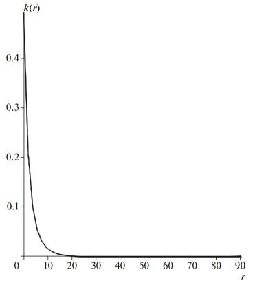
Figure 1: Form of the nodeless regular solution corresponding to the ansatz A

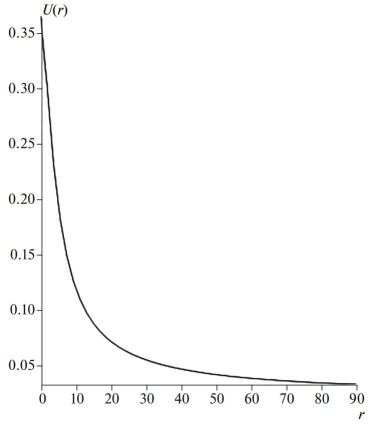
Figure 2: Form of reduced electric potential for the nodeless solution corresponding to the ansatz A

Then, for the found $\beta_{0}$ we integrate the equation for magnetic potential in (25), choosing such value of $\gamma_{0}$ for the ‘‘derivative $\lambda^{\prime}$ at zero’’, for which the growing term in the asymptotic $\lambda\sim Hr+\mu/r^{2}$ approximately vanishes at large distances from the center; then we determine the magnetic moment of the distribution $\mu=r_{0}^{2}\lambda(r_{0})$, making sure that with good accuracy $\mu\approx 1$ (see (28)). The sought form of the magnetic potential for the nodeless solution is shown in Fig. 3.

Figure 3: Form of a magnetic potential for the nodeless solution for the ansatz A

Eventually, using all found values of $\{\beta_{0},\delta_{0},\gamma_{0}\}$, we find the integral characteristics of the nodeless solution by numerical integration, and verify the accuracy of their determination by satisfaction of the integral identities (compare, for example, (35) and (36)). Finally, using the potential $U$ asymptotic, we determine the eigen value for the “reduced frequency” $\varepsilon\approx U(r_{0})+r_{0}U^{\prime}(r_{0})$, and then calculate the binding energy using formula (35).

It can be easily seen that a similar procedure can be applied for finding regular solutions with an arbitrary number of given nodes $N$ of the main function $k(r)$. To this end, it is necessary to narrow down the corresponding interval of $\beta_{N}$ values, allowing the function $k(r)$ to change sign $N$ times. Figure 4 shows the normalized regular solution with the number of nodes $N=2$, as an example.

Table 1 gives the numerically calculated parameters and characteristics of normalized regular solutions to system (44) (and corresponding solutions to (25)) with the number of nodes $N=0\div 10$. It can be seen from Table 1 and Fig. 5 that the values of the binding energy $W_{B}$ reproduce the canonical Bohrian distribution with good accuracy,

$$W_{n}=W/n^{2},\leavevmode\nobreak\ \leavevmode\nobreak\ n=N+1=1,2,....$$ (47)

The next column of Table 1 shows the corresponding values of the binding energy $W^{var}$, obtained by the variational method. Variation was performed in the class of trial functions corresponding to the canonical linear quantum mechanics problem (when the potential of the self-field $\phi(r)$ is not included in the first of Eqs. (44) and $U(r)=\varepsilon=const$):

$$k_{N}=const\cdot L_{N}^{(1)}(x)e^{-x/2},\leavevmode\nobreak\ \leavevmode\nobreak\ x:=r/N,\leavevmode\nobreak\ \leavevmode\nobreak\ N=0,1,2,...,$$ (48)

where $L_{N}^{(1)}(x)$ – are the generalized Laguerre polynomials of power $N$ as a function of $x$, and the eigen values of the corresponding linear problem are

$$\varepsilon_{N}=\frac{1}{4(N+1)^{2}}.$$ (49)

The corresponding trial functions $\phi_{n}(r)$ for the eigen field potential were found by integration of the second equation in (44) with the right-hand part corresponding to (48), so that

$$\phi_{N}^{\prime\prime}+\frac{2}{r}\phi_{N}^{\prime}=k_{N}^{2}.$$ (50)

The corresponding action functional was varied over two parameters of trial functions (48) and (50), namely, the amplitude and scale parameters. Good agreement of the results obtained using the numerical and variational methods can be explained by the fact that inclusion of the electron self-field potential does not qualitatively change the behavior of the functions and their asymptotics both near zero and for large values of radial coordinate.

For solutions with a large number of nodes $N=50\leavevmode\nobreak\ (n=51)$ and $N=100\leavevmode\nobreak\ (n=101)$ the calculations were performed using the variational method alone. In this case, the binding energy still corresponds to Bohr’s law (47) with good accuracy..

It can be seen from Table 1 (see the last column) that the average value of the constant $W$ in (47) is approximately $W\approx 0.120$. The spectrum of dimensional binding energy for (35) or, equivalently, (36) takes the form

$$W_{B}=4RW/n^{2}\approx 0.48R/n^{2}.$$ (51)

Therefore, the effective Rydberg constant $R$ is approximately twice as small as the experimentally observed one. The spectrum of regular solutions with angular dependence corresponding to the ansatz $\bf B$, (see (22)) is found similarly by numerical and variational methods. In this case, system for the radial functions (44) is replaced by the following system if Eq. (19) is used:

$$\begin{array}[]{l}k^{\prime}+(2/r)k=-n,\leavevmode\nobreak\ \leavevmode\nobreak\ n^{\prime}=-(U-(1/r))k\\ \mapsto k^{\prime\prime}+(2/r)k^{\prime}-(2/r^{2})k=(U-(1/r))k,\\ U^{\prime\prime}+(2/r)U^{\prime}=-k^{2},\\ \end{array}$$ (52)

with the asymptotics of the form

$$k\sim\beta r-...,\leavevmode\nobreak\ \leavevmode\nobreak\ n\sim-3\beta+...,\leavevmode\nobreak\ \leavevmode\nobreak\ U\sim\delta-\frac{1}{20}\beta r^{4}$$ (53)

for $r\sim 0$; for $r\rightarrow\infty$ we have

$$k\sim Ae^{-\sqrt{\varepsilon}r},\leavevmode\nobreak\ \leavevmode\nobreak\ n\sim\sqrt{\varepsilon}k,\leavevmode\nobreak\ \leavevmode\nobreak\ U\sim\varepsilon+q/r.$$ (54)

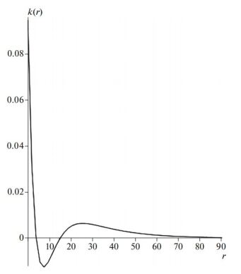
Figure 4: Form of two-node (N = 2) regular solution corresponding to the ansatz A

Variation was performed in the class of trial functions $k(r)$, corresponding to the particular value of the “orbital” quantum number $l=1$ of solutions of the linear canonical quantum mechanical problem, namely, ($2l+1=3$):

$$k_{N}=const\cdot L_{N}^{(3)}(x)e^{-x/2},\leavevmode\nobreak\ \leavevmode\nobreak\ x:=r/N,\leavevmode\nobreak\ \leavevmode\nobreak\ N=0,1,2,...,$$ (55)

for which the eigen values are

$$\varepsilon_{N}=\frac{1}{4n^{2}},\leavevmode\nobreak\ \leavevmode\nobreak\ \leavevmode\nobreak\ n=N+l+1=N+2,$$ (56)

while the eigen potential was determined by trial functions found by integrating former Eq. (50) with the right-hand part defined now by (55).

Table 2 gives the results of the numerical and variational studies of the spectrum of ground and excited states of regular solutions to system (52), which again mutually prove each other.

Figure 5: Binding energy $W_{n}$ of regular solutions for the ansatz A as a function of the “principal quantum number” $n=N+1$ according to (squares) the numerical and (stars) variational methods

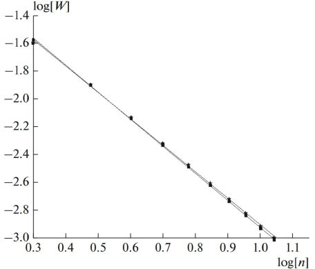
Figure 6: Binding energy $W_{n}$ of regular solutions for the ansatz B as a function of the “principal quantum number” $n=N+2$ according to (squares) the numerical and (stars) variational methods

It follows from this table and Fig. 6 that the Bohrian distribution

$$\ W_{n}=W/n^{2},\leavevmode\nobreak\ \leavevmode\nobreak\ \leavevmode\nobreak\ n=N+2=2,3,...$$ (57)

is again satisfied with a good accuracy, especially for solutions with a large number of nodes $N$. Moreover, the quantity $W$ again has the value $W\approx 0.120$, so the effective Rydberg constant turns out universal, approximately equal to its value for the ansatz $\bf A$ (nearly two times smaller than its experimental value).

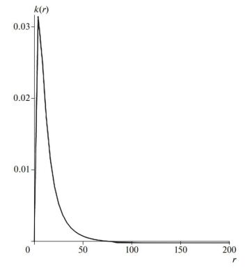
Figure 7: Form of the nodeless regular solution for the ansatz B

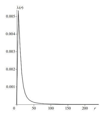
Figure 8: Form of a magnetic potential for the nodeless solution corresponding to the ansatz B

The form of nodeless solution to system of equations (52) is given in Fig. 7 (the cut-off radius is $r_{0}\sim 200$). The corresponding magnetic potential is shown in Fig. 8. Note finally that the values of energies of the states of classes A and B with the same value of the “principal quantum number” $n=N+l+1$ are close to each other, especially for large $n$. Nonetheless, the difference between them, in particular, between the energies of analogs of states $2s_{1/2}$ and $2p_{1/2}$ (for $n=2$, $l=0,1$ respectively) exceeds the experimentally observed one (corresponding to the “Lamb shift”) by many orders of magnitude.

Table 1. Parameters and characteristics of regular solutions for ansatz A.

$$\begin{array}[]{lccccccc}n&\beta=k(0)&\delta=U(0)&\varepsilon=U(\infty)&W_{n}&W_{n}^{var}&W_{n}\cdot n^{2}&W_{n}^{var}\cdot n^{2}\\[7.0pt] 1&0.492787&0.365947&0.02311&0.1218&0.1182&0.1218&0.1182\\ 2&0.17379&0.09042&0.004515&0.03030&0.03056&0.1212&0.1222\\ 3&0.09471&0.04005&0.001338&0.01335&0.01366&0.1201&0.1229\\ 4&0.06135&0.02243&0.0006103&0.007443&0.007696&0.1191&0.1231\\ 5&0.04382&0.01431&0.0003339&0.004757&0.004930&0.1189&0.1233\\ 6&0.03333&0.009921&0.0002028&0.003200&0.003425&0.1187&0.1233\\ 7&0.02639&0.007278&0.0001344&0.002418&0.002517&0.1185&0.1233\\ 8&0.02158&0.005366&0.00009089&0.001849&0.001927&0.1183&0.1234\\ 9&0.01808&0.004394&0.00006706&0.001461&0.001523&0.1183&0.1234\\ 10&0.01542&0.003556&0.00004866&0.001182&0.001234&0.1182&0.1234\\ 11&0.01336&0.002937&0.00003744&0.0009755&0.001020&0.1180&0.1234\\ ...&...&...&...&...&...&....&....\\[7.0pt] 51&.....&.......&......&......&4.745\cdot 10^{-5}&....&0.1234\\ 101&.....&.......&......&......&1.210\cdot 10^{-5}&....&0.1234\end{array}$$

Table 2. Parameters and characteristics of regular solutions for ansatz $\bf B$.

$$\begin{array}[]{lccccccc}n&\beta=k(0)&\delta=U(0)&\varepsilon=U(\infty)&W_{n}&W_{n}^{var}&W_{n}\cdot n^{2}&W_{n}^{var}\cdot n^{2}\\[7.0pt] 2&0.020682&0.07992&0.001025&0.02664&0.02534&0.1066&0.1014\\ 3&0.013741&0.03797&0.000705&0.01266&0.01272&0.1139&0.1145\\ 4&0.009477&0.02178&0.000400&0.007256&0.007407&0.1161&0.1185\\ 5&0.006960&0.001405&0.000253&0.004682&0.004813&0.1174&0.1203\\ 6&0.005366&0.009791&0.000168&0.003264&0.003369&0.1175&0.1213\\ 7&0.007205&0.004292&0.000116&0.002402&0.002487&0.1177&0.1219\\ 8&0.003530&0.005524&0.0000861&0.001842&0.001910&0.1179&0.1222\\ 9&0.002966&0.004367&0.0000618&0.001455&0.001512&0.1179&0.1225\\ 10&0.002540&0.003539&0.0000492&0.001180&0.001227&0.1179&0.1227\\ 11&0.002205&0.002925&0.0000379&0.0009751&0.001015&0.1180&0.1228\\ 12&0.001938&0.002458&0.0000285&0.0008194&0.0008535&0.1180&0.1229\\ ...&...&...&...&...&...&....&....\\[7.0pt] 52&.....&.......&......&......&4.563\cdot 10^{-5}&....&0.1234\\ 102&.....&.......&......&......&1.186\cdot 10^{-5}&....&0.1234\end{array}$$

6 DISCUSSION OF RESULTS

It was already noted that consideration of the electric self-field of the electron in the hydrogen atom looks quite justified, if not inevitable, both from the general physical point of view, and according to the QED ideas. The mathematical structure of the system of Dirac-Maxwell equations becomes quite different from the canonical one; this system is now coupled and effectively nonlinear.

The spectrum of regular states of such a system can be rather reliably determined by numerical and variational methods only for the “nonlinear analogs” of s- or p-states. Indeed, only in these cases successive terms in the chain of equations for the radial functions have increasing order of smallness with respect to the fine structure constant. In the nonrelativistic approximation $\alpha\rightarrow 0$ only the principal harmonics corresponding to the orbital quantum number $l=0,1$, contribute to the binding energy. It is possible to obtain relativistic corrections determined for the same solutions by harmonics with higher values of $l$ and corresponding harmonics of electric and magnetic potentials of the electron; however, it requires cumbersome calculations and is not considered here (estimations were obtained in [25]).

Thus, the solutions and the binding energy spectrum given in this paper should actually be compared with solutions to the Schrödinger equation of s- and p-types in the presence of the external Coulomb field. Surprisingly, quite a different structure of the considered nonlinear model reproduces the canonical Bohrian distribution with good accuracy, and the better, the larger “principal quantum number” is considered. The effective Rydberg constant turns out to have very close values for both classes of solutions, thus, it can be assumed universal. The spinor “wave function” normalization condition is satisfied as a direct consequence of the natural electroneutrality condition, and the (projection) of the total angular momentum turns out exactly equal to $\pm\hbar/2$.

Unfortunately, at this point coincidences with quantum mechanics and experiment cease. The numerical value of the “Rydberg constant” is approximately twice as small as the observed one, and the “Lamb shift” is larger than the observed one by many orders of magnitude. Also, the magnetic moment of distributions corresponding to the “analogs” of p-states, strangely, is three times smaller than the magnetic moment of the electron. It is possible, of course, following  [18] to transform the discovered spectrum of levels using the classical analog of the renormalization procedure that would have nothing to do with subtracting of infinities, like in QED, but would be reduced to simply equating the observed electron mass to the doubled initial mass of the bare particle $m$ in the Dirac equation. However, this trick, obviously, does not solve all problems of agreement between the obtained results and experiment, including the value of magnetic moment of the ansatz B and the anomalously large difference between the energies of levels $2s_{1/2}$ and $2p_{1/2}$.

In general, it seems that complete agreement with experiment, including radiative corrections, is possible in the framework of a purely classical field model of the hydrogen atom free of any divergences and the use of second quantization. For this purpose, however, it is necessary to consider a certain additional factor, for example, self-action with respect to the spinor field [30] or possible supersymmetric structure of the considered self-consistent model [2]. We leave more detailed discussion of these issues for later.

7 ADDENDUM

In the reviewing process, a paper by Ranãda and Uson  [31] was found, which is very close both with respect to the problem formulation, methods of study, and results obtained . Namely, in essence, a similar hydrogen atom model accounting for the electric self-field of the electron represented by the self-consistent system of Dirac-Maxwell equation with Lagrangian (1) was considered. The same stationary regular solutions related to the nonlinear analogs of s- and p-states and corresponding to our ansatzes A and B, respectively, were sought.

However, instead of direct reduction to the nonrelativistic case based on transformation (15) and subsequent $\alpha$-expansion (Section 3), a cumbersome procedure of the numerical integration of initial system (14) (in the unsubstantiated assumption on the smallness of terms with magnetic potential in the equations for spinor harmonics) was applied in [31].

Nonetheless, for the first three levels 1s, 2s, 3s and two levels  1p, 2p the results obtained in  [31] agree with those given above (Tables 1 and 2) with good accuracy. For example, for the energy $E$ of the ground state 1s, according to formula (26) from [31], one finds, up to corrections $\sim\alpha^{4}$):

$$E=mc^{2}(1-0.243894\alpha^{2}),$$ (58)

which, similar to our study, corresponds to the binding energy $W_{B}\approx R/2$ and is approximately twice as small as the experimental value. For the first three s-levels they have, with good accuracy, Bohrian function for the binding energy (47) (our result is first 10 levels in the case of the numerical method, and up to $n=100$ in the case of the variational method). The results for the first two p-states considered in [31], also agree well with the above data.

Correspondingly, the conclusion made in [31] is similar to ours. Namely, in spite of the physically grounded statement of the problem, the results do not improve but violate the agreement with the linear quantum mechanical problem and experiment. In this relation, similar to  [18], it is proposed in [31] to apply the classical analog of the renormalization procedure by a corresponding redefinition of the coupling constant $e$ and the “bare” mass $m$, in order to formally agree with the observed parameters. In this case, it is possible to provide correct values for the energy difference and absolute values for the first three s-levels. According to the authors, for p-states the results of reconciliation are not quite satisfactory.

Unfortunately, as it was already noted above (Section 6), in the considered model, the charge/mass renormalization is in principle incapable of solving the problem of achieving agreement with experiment. Obviously, say, it cannot change the ratio of magnetic moments of the particle in s- and p-state $M_{s}/M_{p}=3$, or the anomalously large difference between the binding energies for $2s_{1/2}$ and $2p_{1/2}$ states. Note that in [31] these effects were not discovered at all.

Moreover, the absolute values of the mechanical $J$ and magnetic $M$ moments of the particle change in the case of renormalization proposed in [31]. For example, for s-states we have

$$J=XJ_{0},M=XM_{0},\leavevmode\nobreak\ \leavevmode\nobreak\ J_{0}:=\frac{\hbar}{2},\leavevmode\nobreak\ M_{0}=\frac{e_{0}\hbar}{2m_{0}c},\leavevmode\nobreak\ \leavevmode\nobreak\ X:=\frac{e_{0}}{e}\equiv\frac{m_{0}}{m},$$ (59)

where $e_{0},m_{0}$ are the electron charge and mass, respectively, and $e,m$ are the bare charge and mass, i.e., the corresponding scaling factors in initial Lagrangian (1). For formal agreement of the energy of s- and p-states with experiment, the normalization $X$ should be taken as follows: $X^{2}\approx 2$. This scale transformation results thus in incorrect values of the mechanical and magnetic moments, which was not noticed in [31]

Finally, charge/mass renormalization violates the normalization condition of the particle spinor field (3), which prevents us from considering it as the “wave function”; it also violates the agreement of the model with the linear quantum theory on the whole. Summing up the above said, it should be admitted that in the form considered here and in [31] the Dirac-Maxwell model, being mathematically correct and extremely rich with respect to its inner properties, is unsatisfactory from the physical point of view and should be substantially changed. Note in this regard, that in  [31] an important conclusion on a negligibly small effect of self-action with respect to the spinor field (proposed above, see Section 6) on the hydrogen spectrum was made. The grounds for this conclusion are both the results of the numerical integration and qualitative considerations on large spatial extension of the Dirac field ($>10^{-8}$ cm) in the hydrogen atom, i.e., extension to the region where the nonlinear term is negligible. Thus, other possibilities for the model modification should be used. We expect to discuss and consider some of them in the future.

8 ACKNOWLEDGMENTS

We thank A.B. Pestov, Yu.P. Rybakov, and B.N. Frolov for helpful discussions and bibliographic indications.

9 FUNDING

The work was supported by the “University program 5-100” of the Russian Peoples’ Friendship University.

References

- [1] G. A. Zaitsev, Algebraic Problems of Mathematical and Theoretical Physics, (Nauka, Moscow, 1974) [in Russian], pp. 158–163.
- [2] A. Wipf, A. Kirchgerg, D. Lange, Algebraic solution of the supersymmetric hydrogen // Bulg. J. Phys. – 2006. – V. 11. – P. 206-216. – arXiv:0511.1231 [hep-th].
- [3] L. de la Peria, A.M. Cetto A, A. Valdes-Hernandes, The zero-point field and the emergence of the quantum // Int. J. Mod. Phys. E – 2014. – V. 23 (09). – P. 145009.
-
[4]
Yu. P. Rybakov, Solitons and quantum mechanics //
Dynam. Compl. Syst. – 2009. – V. 4. – P. 3–15;
Yu.P. Rybakov, B. Saha, Interaction of a charged 3D soliton with a Coulomb center // Phys. Lett. A. – 1996. – V. 222. – P. 5 -13. – arXiv:9603004 [atom-ph]. - [5] J.-P. Vigier, An electromagnetic theory of strong interactions // Phys. Lett. A. – 2003. – V. 319. – P. 246-250.
- [6] N.V. Samsonenko, D.V. Tahti, F. Ndahayo, On the Barut-Vigier model of the hydrogen atom // Phys. Lett. A. – 1996. – V. 220. – P. 297-301.
- [7] A. D. Vlasov, The Shrödinger atom // Phys. Usp. – 1993. – V. 36. – P. 94–99.
- [8] L. P. Pitaevskii, On the problem of the “Shrödinger atom” // Phys. Usp. – 1993. – V. 36. – P. 760–761.
- [9] L. Diosi, Gravitation and quantum-mechanical localization of macroobjects // Phys. Lett. A. – 1984. – V. 105. – P. 199 -202.
- [10] R. Penrose, On gravity’s role in quantum state reduction // Gen. Relat. Grav. – 1996. – V. 28. – P. 581-600.
- [11] I.M. Moroz, R. Penrose, K.P. Tod, Spherically symmetric solutions of the Schrödinger - Newton equations // Class. Quant. Grav. – 1998. – V. 15. – P. 2733 - 2742.
- [12] W. Heitler, The Quantum Theory of Radiation (Oxford University Press, 1936).
- [13] A. I. Akhiezer, V. B. Berestetskii, Quantum Electrodynamics (Nauka, Moscow, 1969) [in Russian].
- [14] P.J. Mohr, Self-energy correction to one-electron energy levels in a strong Coulomb field // Phys. Rev. A. – 1992. – V. 46. – P. 4421 - 4424.
- [15] A.O. Barut, Y.I. Salamin, Relativistic theory of spontaneous emission // Phys. Rev. A. – 1988. – V. 37. – P. 2284 - 2296.
- [16] A.O. Barut, J. Kraus, Y. Salamin, N. Ünal, Relativistic theory of the Lamb shift in self-field quantum electrodynamics // Phys. Rev. A. – 1992. – V. 45. – P. 7740 - 7745.
- [17] I. Acikgoz, A.O. Barut, J. Kraus, N. Ünal, Self-dual quantum electrodynamics without infinities. A new calculation of vacuum polarization // Phys. Lett. A. – 1995. – V. 198. – P. 126 - 130.
- [18] G.N. Afanas’ev, V.G. Kartavenko, A.B. Pestov, Coulomb self-action effect on shift of atomic levels // Bull. Rus. Acad. Sci. Phys. – 1994. – V. 58. – P. 738-752 .
- [19] N. Rosen, A field theory of elementary particles // Phys. Rev. – 1939. – V. 55. – P. 94-101.
- [20] M. Wakano, Intensely localized solutions to the classical Dirac-Maxwell field equations // Prog. Theor. Phys. – 1966. – V. 36., no. 6. – P. 1117-1141.
- [21] V.V. Kassandrov, Spin and charge of solitons in the model of interacting electromagnetic and spinor fields // Vestnik Peoples’ Friend. Univ. – 1995. –no. 3. – P. 168–174.
- [22] A.P. Kostyuk, I.M. Chepilko, Spherically symmetric electrostatic solitons of Klein–Gordon and Dirac fields // Phys. Atom. Nucl. – 1993. – V. 56. – P. 233–247.
- [23] C. Seam Bohum, F.I. Cooperstock, Dirac-Maxwell solitons // Phys. Rev. A – 1999. – V. 60. – P. 4291-4300. – arXiv:0001038 [physics].
- [24] V. V. Kassandrov, Discrete Characteristics of Particles in Nonlinear Classical Field Theories // D.Sc. Thesis (Peoples’ Friend. Univ., Moscow, 1977).
- [25] V.V. Kassandrov, Solitons in classical spinor electrodynamics under the presence of an external field // In: “ Statistical Physics and Field Theory” (Peoples’ Friend. Univ., Moscow, 1990). P. 48-53.
- [26] L.V. Biguaa, V.V. Kassandrov, Soliton model of the hydrogen atom // In: “Proceedings of LV All-Russian Conference on the Problems of Dynamics, Particle Physics, Plasma Physics and Optoelectronics” (Peoples’ Friend. Univ. Russia, Moscow, 2018), P. 17–21.
- [27] E. Schrödinger, Selected Papers on Quantum Mechanics (Nauka, Moscow, 1976) [in Russian].
- [28] D.H. Bernstein, E. Giladi, K.R.W. Jones, Eigenstates of the gravitational Schrödinger equations // Mod. Phys. Lett. A – 1998. – V. 13. – P. 2327-2336.
- [29] D. Ivanenko, A. Sokolov, Classical Field Theory (New Problems) (GITTL, Moscow, 1949) [in Russian]. Ch. 4.
- [30] M. Soler, Classical electrodynamics for a nonlinear spinor field: perturbative and exact approaches // Phys. Rev. D. – 1973. – V. 8. – P. 3424 - 3429.
- [31] A.F. Ranãda, J.M. Uson, Bound states of a classical charged nonlinear Dirac field in a Coulomb potential // J. Math. Phys. – 1981. – V. 22. – P. 2533 - 2538.