Remarks on generating realistic synthetic meteoroid orbits

Abstract

Context. To identify the real associations of small bodies, we can use synthetic sets of orbits generated by various methods. These are not perfect methods, therefore the assessment of their quality is an essential task.

Aims. In this study, we compared five methods for generating synthetic meteoroid orbits. Three of them (ME0, KD10, and KDns) had already been proposed in the literature, while two additional ones (ME1 and ME4) are new methods.

Methods. As far as possible, the synthetic orbits were compared with the orbits of the observed meteoroids. For quantitative comparison, we applied a few tests: the $\chi^{2}$-distance and the nearest neighbor $NN_{N}$ tests used in previous works, and one-dimensional $\chi^{2}$ and Kolmogorov-Smirnov (K-S) tests, as well as a two-dimensional K-S test implemented in this study. To estimate a general property of the orbital sample, we proposed the use of the entropy $H_{N}$ of the data set based on the nearest neighbor distances. Finally, we did a cluster analysis of the synthetic orbits. We calculated and compared the values of the orbital similarity thresholds.

Results. We showed that generating ’realistic’ meteoroid orbits and testing their quality is a complex issue. An assessment of the quality of the generated orbits depends on the type of test applied, and it refers to the sample of the observed orbits used. Different tests give different assessments. However, in practice, the investigated methods produced similar results if they were applied correspondingly.

1 Introduction

Searching for streams among meteoroid orbits, including an assessment of their reliability, is based heavily on the artificial orbital samples derived by means of the statistical properties of the observed orbital elements. One can derive the synthetic orbital samples, free from clusters, by different methods (see, for example, Jopek & Froeschlé (1997), Jopek et al. (2003), Pauls & Gladman (2005), Koten et al. (2014), Guennoun et al. (2019)). Recently, Jopek & Bronikowska (2017) have shown that the choice of the method used for generating synthetic orbits impacts the assessment of the probability of spurious pairings. Jopek & Bronikowska (2017) tested a few methods and, in the case of meteoroid orbits, they recommend their method as the most reliable. However, Vida et al. (2017) found some drawbacks of this method, and concurrently they proposed an interesting approach based on the Kernel Density Estimation method (KD method).

In this study, we describe an improvement of method E, by eliminating the drawbacks pointed out by Vida et al. (2017), and by introducing into the algorithm a few additional steps that more precisely allow for the correlations between the meteoroid orbital elements. The modified methods have been compared with the KD methods proposed by Vida et al. (2017).

2 Orbital data used in this study

In this study, the same meteoroid data have been used as in Vida et al. (2017), namely, the file CAMS-v2-2013.csv (see Jenniskens et al., 2016) downloaded from the GitHub site (https://github.com/dvida/GenMeteorSporadics). We used the heliocentric ecliptical osculating orbital elements $q,e,\omega,\Omega,i$ and the ecliptic latitude $\beta_{G}$ of the meteor geocentric radiants. Additionally, we use the heliocentric distances of the Earth $R_{E}$, calculated at the moment of meteor observations by means of the formula taken from Bell & Urban (2012). Using the software posted by Vida et al. (2017) at the GitHub site, from the original CAMS file, we extracted $58029$ orbits of sporadic meteors, which we considered to be an orbital sample free from clusters.

3 Synthetic meteoroid orbits generation methods

In this study, we compared a few methods: ME0 (method E in Jopek & Bronikowska (2017)) and its two variations ME1 and ME4. The ME methods use the CPD (cumulative probability distribution) inversion technique parametrized by the choice of the bin width of the histogram used for each orbital element. In the ME0 method, it is assumed that the Earth moves in a circular orbit around the Sun. The ME1 method is based on the ME0 method, in which the assumption of the elliptical orbit of Earth was introduced. In turn, the ME4 method is an extended version of the ME1 method. The values of the argument of perihelion $\omega$ were generated by the CPD technique using not one marginal distribution but two, corresponding to the positive and negative ecliptic latitudes of the meteor radiants.

Additionally, we made use of three KD methods: KD0.1, KD10, and KDns (see, Vida et al. (2017)). The KD methods use the nonparametric technique; they are based on the multivariate kernel density estimation. The methods depend on the choice of the bandwidth matrix $H$. This matrix has a decisive influence on the shape (smoothness) of the obtained multivariate probability distribution function. In the work of Vida et al. (2017), three diagonal H matrices were used, two scalar matrices with elements equal to $0.1$ and $10$ (methods KD0.1 and KD10 respectively) and one non-scalar matrix (KDns method) with elements selected separately for each orbital element. More details about the applied ME and KD methods are provided in the Appendix.

4 Valuation of the synthetic orbital sample

4.1 Comparison of the observed and synthetic samples

The ME method uses the marginal densities represented by the marginal histograms of the observed orbital elements (see Fig. 1). The application of the CPD inversion technique guarantees that the marginal distributions of the synthetic and observed orbital elements are very similar. However, this technique does not conserve the correlations between the meteoroid orbital elements $q,e$, and $\omega$ (see Fig. 2). To address these correlations, Jopek & Bronikowska (2017) added steps 2 and 3 to the ME0 method (see Appendix A.1). However, in their paper no comparisons between the obtained synthetic and observed samples were accomplished, except for a visual assessment.

In Vida et al. (2017), to ascertain the differences or similarities between the observed and synthetic orbital sets, a few comparisons were accomplished, namely, a visual comparison of 1D or 2D histograms of the observed and synthetic orbital elements, and a limited quantitative assessment of the similarity between observed and synthetic samples. For this purpose, Vida et al. (2017) used the 2D histogram of $\omega$ versus $q$, for which the so-called $\chi^{2}$ histogram distance was calculated (see Pele & Werman, 2010) using

$$\chi^{2}(P,Q)=0.5\sum_{i=1}^{k_{\omega}}\sum_{j=1}^{k_{q}}\frac{(P_{ij}-Q_{ij})^{2}}{(P_{ij}+Q_{ij})},$$ (1)

where $P_{ij}$ and $Q_{ij}$ are the contents of the $ij$ bins of the synthetic and observed data histograms, respectively. The number of bins are represented by $k_{\omega}$ and $k_{q}$ .

In Vida et al. (2017), as an additional statistical property of the sample, the arithmetic mean ${NN_{N}}$ of the nearest neighbor distances was calculated, which is the averaged minimum distance from each orbit to any other for a given sample. Let $D_{N,i}$ be the nearest neighbor distance of the orbit $O_{i}$ and the other $O_{j}$: $D_{N,i}=\min_{j\neq i,j\leq N}\,D(O_{i},O_{j})$, then

$${NN_{N}}=\frac{1}{N}\sum_{i=1}^{N}D_{N,i},$$ (2)

where $N$ – is the sample size. To determine the distance $D(O_{i},O_{j})$ between two orbits, the $D_{SH}$-function was applied (see, Southworth & Hawkins, 1963).

As a statistical property between two orbital samples, Vida et al. (2017) calculated the arithmetic mean ${OS_{N}}$ of the smallest D-values between each synthetic orbit paired with each observed orbit.

To compare the two orbital samples, in the present work we have used ideas from Vida et al. (2017), expanding them slightly, as well as additional new ideas, namely we compared the marginal distributions of $q,e,\omega,\Omega,i$ as well as the 2D distributions of all pairs of orbital elements using the $\chi^{2}$ and Kolmogorov-Smirnov (K-S) tests taken from Press et al. (2002). The advantage of this approach is the ability to estimate whether the compared samples could come from the same population.

To assess the general similarity of orbital samples, we used the concept of entropy. As far as we know, this concept has never been used for this purpose. The entropy $H_{N}$ was calculated on the basis of the nearest neighborhood values $D_{N,i}$. For each point in the sample, one has to find the distance to its nearest neighbor and apply the formula (Beirlant et al., 1997)

$$H_{N}=\frac{1}{N}\sum_{i=1}^{N}\left[\ln(N\cdot D_{N,i})\right]+\ln(2)+C_{E}$$ (3)

where $C_{E}=0.577215664901532860...$ is the Euler constant. An analogy between ${NN_{N}}$ and $H_{N}$ is clearly seen.

Finally, we propose a purely practical approach. For the synthetic orbits, we compared the orbital similarity thresholds used in the cluster analysis. We determined the thresholds by a single linkage cluster analysis and three $D-$functions. More details of this procedure are given in Jopek (2020).

In the next section, we present the results of our calculation of the $\chi^{2}$ distances and ${OS_{N}}$, ${NN_{N}}$ statistics, as well as the results of the $\chi^{2}$ test and K-S test, using the observed and synthetic data sets. Moreover, we present the values of the entropy and orbital similarity thresholds calculated for the synthetic orbital samples.

4.2 Results of comparison and discussion

In this section, we present the results of quality tests on synthetic sets of $58029$ and $29014$ orbits. First, tests carried out by Vida et al. (2017) were repeated. The following sections present the results of the extended comparison of reduced orbital samples. The last section describes the results of the cluster analysis among the generated orbits.

4.2.1 Samples comprising 58029 orbits

At this stage, we only recalculated the results already obtained by Vida et al. (2017) that are provided in their Table 1. Exploiting the software placed by Vida et al. on the GitHub website, we generated four synthetic samples and calculated their $\chi^{2}$ distances and ${OS_{N}}$, ${NN_{N}}$ statistics (see our Table LABEL:tab:comparison1).

Table 1: The $\chi^{2}$ distances and ${SO_{N}}$, ${NN_{N}}$ statistics calculated for $58029$ orbits, observed and generated by the ME method and three variations of the KD method, see text. In the second column, the $\chi^{2}$ distances were calculated using $\omega$-$q$ histograms with $158$x$103$ bins. Additionally, in the third column the $\chi^{2}$ distances were determined using $80$x$80$ bins, see text.

Orbital sample	$\chi^{2}$ distance		${OS}_{N}$	${NN}_{N}$
	158x103	80x80
CAMS 58029	-	-	-	0.0806
ME	19053	16285	0.0995	0.1008
KD10	16376	14048	0.0821	0.0896
KD0.1	1858	933	0.0408	0.0447
KDns	9189	6921	0.0776	0.0840

The $\chi^{2}$ distances given in the second column of Table LABEL:tab:comparison1 were obtained using $q$ versus $\omega$ histograms with $158$x$103$ bins, as used in Vida et al. (2017). Our results differ slightly from those found by Vida et al. (2017) due to two reasons: we used corrected software, and we used a different sequence of random values starting with the seed point $2003$.

As in Vida et al. (2017), in Table LABEL:tab:comparison1 the largest $\chi^{2}$ value was obtained for the ME sample, the smallest value for the KD0.1 sample. However, we must point out that the $\chi^{2}$ distances given in Table LABEL:tab:comparison1 have no clear interpretation. The high value $\chi^{2}$=$19053$ does not necessarily mean that in some applications the ME synthetic sample cannot effectively represent the observed orbits. On the other hand, one may ask, does the smallest value $\chi^{2}$=$1858$ indicate that the synthetic sample generated by the KD0.1 method is too similar to the observed one?

Furthermore, the $\chi^{2}$ distance considerably depends on the number of applied bins. This is shown in the third column of Table LABEL:tab:comparison1 where we placed the $\chi^{2}$ distances calculated using histograms with $80$x$80$ bins. The number of bins was calculated according to the Rice Rule: $k=\lceil 2N^{1/3}\rceil$, where $\lceil\ldots\rceil$ is the ceiling function and $N$ is the sample size. The obtained $\chi^{2}$ distances differ significantly from those given in the second column of Table LABEL:tab:comparison1. Hence, the question may arise, which $\chi^{2}$ value should be used to valuate the quality of a synthetic sample? Thus, we believe that the $\chi^{2}$ value determined by Eq. (1) should be used with care for the adjudication of a synthetic orbits generator.

In Vida et al. (2017), the authors used another statistics for a quantitative comparison of the observed and synthetic samples. As was mentioned in Sect. 4.1, the authors proposed two statistics: the arithmetic means ${NN_{N}}$ and ${OS_{N}}$. We also calculated ${NN_{N}}$ and ${OS_{N}}$ and the obtained results are given in Table LABEL:tab:comparison1. Our results differ slightly from those given in Table 1 in Vida et al. (2017) for the same reasons as those we mentioned earlier. The highest values of ${NN_{N}}$ and ${OS_{N}}$ are for the ME sample. Vida et al. (2017) considered the ${OS_{N}}=0.0995$ as an upper bound for an acceptable synthetic orbit data set. As the lower bound, Vida et al. considered a value of ${OS_{N}}=0.0408$. Certainly, a low value of ${OS_{N}}$ may imply a strong similarity between the two samples. However, we are interested in a statistical similarity. Therefore, as in the case of the $\chi^{2}$ distance, one may ask, which limit values of ${OS_{N}}$, ${NN_{N}}$ may be relevant to the issue of the comparison between synthetic and observed samples? We address this question in the next section.

4.2.2 Samples comprising 29014 orbits

To find the expected values of the $\chi^{2}$ distances, ${OS_{N}}$ and ${NN_{N}}$ , and other statistics, we split the original CAMS sample into two subsamples, CAMSA and CAMSB, each containing $29014$ orbits. The CAMS sample is sorted by increasing values of the ecliptic longitude of the Sun at a meteor instant, hence to split the data sample we just used the catalog ordinal numbers of orbits: the even-numbered orbit entered sample CAMSA, the odd-numbered entered sample CAMSB.

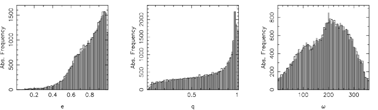
Figure 1: Marginal histograms of the osculating orbital elements of the observed subsamples CAMSA and CAMSB (in gray). Each sample consists of $29014$ orbits, the number of bins is $62$. The distributions display a clear statistical similarity. Except for one small surplus seen in the $\omega$ histogram, the only visible differences are the statistical fluctuations.

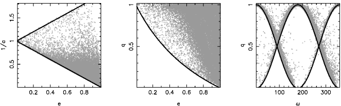
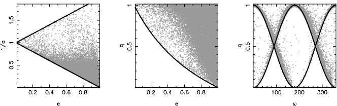
Figure 2: Distributions of $29014$ sporadic video meteoroids (top – CAMSA and bottom – CAMSB subsample) on the $q$-$e$, $(1/a)$-$e$, and $\omega$-$q$ planes. Due to the observation selection effect, not all combinations of $[q,e]$, $[(1/a),e]$, or $[\omega,q]$ are observable from the surface of the Earth.

Table 2: Results of the quantitative comparison of $29014$ observed and synthetic meteoroid orbits. The first section contains the results obtained for the CAMSA and CAMSB subsamples. The second section contains the results determined for synthetic samples generated using CAMSA orbits (see text). The $\chi^{2}$ distances were calculated using $\omega$-$q$ histograms with $62$x$62$ bins. Subsequent columns contain ${OS_{N}}$ and ${NN_{N}}$ statistics.

Orbital sample	$\chi^{2}$ distance	${OS_{N}}$	${NN_{N}}$
CAMSA 29014	-	-	0.097
CAMSB 29014	760	0.096	0.096
Method E	7424	0.119	0.120
KD, h=10	6499	0.094	0.103
KD, h=0.1	473	0.048	0.051
KD, non-scalar	3103	0.089	0.096

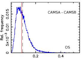
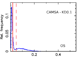
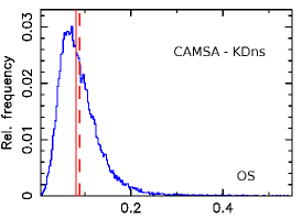
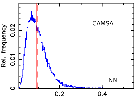
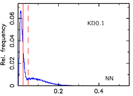
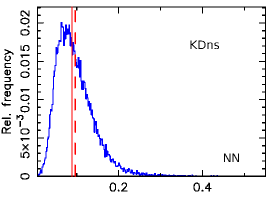
Figure 3: Histograms of the values used to calculate the ${OS_{N}}$ (top) and ${NN_{N}}$ (bottom) statistics. The dashed red lines correspond to the ${OS_{N}}$ and ${NN_{N}}$ mean values, the continuous lines correspond to the median values. The $OS$ histograms were produced using the observed CAMSA and CAMSB orbits (left), the CAMSA and KD0.1 (middle), and the CAMSA and KDns samples (right). The $NN$ histograms correspond to CAMSA, KD0.1, and KDns samples, respectively. For the KD0.1 synthetic data, the histograms are considerably different from the remaining ones.

The CAMSA and CAMSB subsamples were taken from the same ’population’ of the observed orbits, hence their statistical properties should be very similar. In Fig. 1 we see that their marginal distributions of the orbital elements display a clear statistical similarity. This similarity is also visible in the 2D distributions in Fig. 2. This figure shows the effects of observational selection that correlate some elements of the meteoroid orbit. Because a typical meteoroid can be observed only in the form of a meteor phenomenon in the Earth’s atmosphere, an approximate relationship between its orbital elements $q$, $e$, and $\omega$ is often used (see, e.g., Jopek & Froeschlé, 1997; Babadzhanov et al., 2012), namely

$$q={{R_{E}\,(1\pm e\cos\omega)}\over{1+e}},$$ (4)

where $R_{E}$ in astronomical units is the heliocentric distance of a meteoroid at its moment of collision with Earth. The sign at the $e\cos\omega$ is positive for the negative geocentric ecliptic latitude of a meteor radiant, $\beta_{G}<0$. Assuming a circular orbit of the Earth ($R_{E}$=$1$), the relationship $q=f(\omega)$ has been drawn in Fig. 2 in the form of continuous lines. Due to the nonzero eccentricity of the Earth’s orbit, $R_{E}$ belongs to the interval

$$0.9833\leq R_{E}\leq 1.0167,$$ (5)

and as a result, the points corresponding to the observed meteoroids surround the curve for $R_{E}=1$.

If we ignore the size of the Earth, that is, if we assume that meteors are observed at the center of the Earth, then Eq. (4) is exact. Violations of Eq. (4) and Condition (5) do not happen often (see Jopek et al., 2010), but in $58029$ sporadic meteoroid orbits from the CAMS catalog they occurred $\sim$$2000$ times.

Another consequence of the observational selection concerns the values of the meteoroid’s orbital elements $e,q,$ and $1/a$. As we see in Fig. 2, certain combinations of the values of these elements are unacceptable for meteoroids observed from the Earth’s surface. For the given values of $e$ and $R_{E}$, the limit values for $q$ and $1/a$ are

$$q_{max}=R_{E},$$

$$q_{min}=R_{E}\cdot(1-e)/(1+e),$$

$$(1/a)_{max}=1/R_{E}\cdot(1-e),$$ (6)

$$(1/a)_{min}=1/R_{E}\cdot(1+e),$$

where $R_{E}$ belongs to interval (5). Equations (6) describe the boundary curve $q(e)$ and two limits for $(1/a)$ seen in Fig. 2.

The similarity of the 1D and 2D distributions, shown in Figs. 1 and 2, confirms our assumption that both CAMSA and CAMSB samples represent statistical properties of the same population. Therefore, for these samples we calculated the values of the statistics used, and they were applied as the reference values when the synthetic data were evaluated. We repeated the calculations of the $\chi^{2}$ distance, and ${OS_{N}}$ and ${NN_{N}}$ statistics for reduced synthetic samples of $29014$ orbits (see Table LABEL:tab:comparison2). To find the $\chi^{2}$ distances, we used $\omega$-$q$ histograms with $62$x$62$ bins, and the number of bins was calculated according to the earlier mentioned Rice Rule.

In Table LABEL:tab:comparison2, the $\chi^{2}$ values are two to three times smaller than those provided in Table LABEL:tab:comparison1. In Table LABEL:tab:comparison2, the largest $\chi^{2}$ value was calculated for the ME sample, the smallest one corresponds to the KD0.1 sample. Moreover for the ${NN_{N}}$ statistics, the ME sample shows the large difference compared to the observed orbits. However, while it is not the largest one, the largest difference was produced by the KD0.1 method. Vida et al. (2017) interpret the ${OS_{N}}$ and ${NN_{N}}$ as the indicators of statistical similarity between the synthetic and observed samples. However, in comparison with the reference values, the small values ${OS_{N}}=0.048$ and ${NN_{N}}=0.051$ given in Table LABEL:tab:comparison2 do not mean that the KD0.1 sample is statistically very similar to the observed one. This is obvious when we look at Fig. 3. The $NN$ histograms for the observed and KD0.1 samples should look similar, but here the discrepancy is considerable, and we have to admit that we do not know what the reason is. In addition, in Table LABEL:tab:comparison2, for the KD0.1 method the value of the $\chi^{2}$ distance is too small. The $\chi^{2}$=$473$ is smaller than $\chi^{2}$=$760$ calculated for the CAMSA and CAMSB, two samples drawn from the same ’population’.

The ${OS_{N}}$ and ${NN_{N}}$ statistics do not give an unambiguous assessment of the quality of the synthetic orbit generator. As we can see in Table LABEL:tab:comparison2, if we use ${OS_{N}}$ statistics, then method KD10 turns out to be the best; if we choose ${NN_{N}}$ statistics, then method KDns is the best.

In conclusion, we believe that the application of the $\chi^{2}$ distance, and ${OS_{N}}$ and ${NN_{N}}$ statistics only may not be sufficient to decide which synthetic sample more adequately represents the observed data.

4.3 Extended comparison and discussion

To assess whether the synthetic orbital data sets are of acceptable quality, in Vida et al. (2017) the authors used the $\chi^{2}$ distance calculated for $\omega$ and $q$ only, so using only a part of the orbital sample, and as we have shown such a limited approach may not always be applicable. We think that to evaluate the properties of a synthetic orbit generator, one should perform a more comprehensive test that seeks to establish the statistical similarity of two data sets using all five orbital elements. Moreover, from a practical point of view it is essential to compare the results obtained with different synthetic samples used in a specific issue, for example, in a cluster analysis.

In the next section, we present the results of the extended tests of the observed and synthetic data. We also present the results of calculations of the thresholds of orbital similarity, which are key parameters of each cluster analysis using the meteoroid data.

4.3.1 $\chi^{2}$ and K-S statistical tests

Can we prove that two orbital data sets are consistent with a single distribution function? As far as we know, there is no affirmative answer to this question. Hence, we do not have a ready-for-use solution. However, using statistical tests, we can compare the 1D and 2D distributions of the orbital element samples. Hence, in this study, we wanted to find which available statistical tests can be helpful in assessing the quality of the orbital sample generators. We used the $\chi^{2}$ test (not to be confused with the $\chi^{2}$- distance given by Eq. (1)) and two K-S tests. All tests were performed using the subroutines taken from the ‘Numerical Recipes’ package (Press et al., 2002), namely: chstwo, kstwo, and ks2d2s. Each subroutine returns an estimate of the significance prob parameter, which determines the level of consistency between compared distributions. The prob takes values in the range $[0,1]$, however, concerning the critical value of this parameter, in Press et al. (2002) the authors only note that a small value of prob indicates a significant difference between the compared distributions. Hence, to estimate what values of prob can be expected, we performed the $\chi^{2}$ and K-S tests using the observed CAMSA and CAMSB samples.

One-dimensional $\chi^{2}$ tests

Making use of the 1D $\chi^{2}$ test, we compared the marginal distributions of $e,q,\omega,\Omega,i$ orbital elements of the CAMSA sample with CAMSB and synthetic samples. The results of the tests are collected in Table LABEL:tab:chi-KS1. We tested five methods, and their algorithms are described in the Appendix.

Table 3: Results of the 1D $\chi^{2}$ test (first section) and 1D K-S test (second section) for marginal distributions of the orbital elements. We compared the orbits from the observed CAMSA sample with the orbits generated by the KD10, KDns, ME0, ME1, and ME4 methods. The results of a comparison of the CAMSA and CAMSB samples serve as a reference for the other tests.

	CAMSB	KD10	KDns	ME0	ME1	ME4
q	45.7	0.0	0.0	0.0	0.0	0.0
e	35.3	0.0	0.0	67.4	94.0	97.1
i	68.1	4.0	35.7	100.0	96.4	98.3
$\omega$	80.2	0.0	0.7	36.9	20.2	100.0
$\Omega$	100.0	98.4	99.9	99.9	100.0	100.0
	CAMSB	KD10	KDns	ME0	ME1	ME4
q	33.1	0.0	0.0	0.0	0.0	0.0
e	98.4	0.0	0.0	18.0	14.4	65.2
i	78.8	0.0	0.0	48.2	92.8	50.8
$\omega$	31.1	0.2	0.8	57.5	87.7	88.2
$\Omega$	95.9	11.4	87.2	35.7	26.4	58.9

As can be seen in Table 3, the comparison of the marginal distributions of the perihelion distances $q$, gave negative results for all synthetic samples. This is not surprising in the case of ME methods, where $q$ is not generated using its marginal distribution of the observed sample. In each of the ME methods the perihelion distance was calculated using Eq. (4), substituting the generated values of $e$, $\omega$ as well as the heliocentric distance $R_{E}$ of Earth at the moment of time of the meteor observation.
For the remaining orbital elements, the results of the $\chi^{2}$ test are usually more favorable for ME methods. This is due to the fact that KD orbits are not generated on the basis of the marginal distributions. Similarly, one can explain why the prob values for $e,i,$ and partly for $\omega$ tests are lower for the CAMSB sample than for synthetic orbits generated by ME methods. The CAMSA and CAMSB samples were obtained based on the sorted values of the ecliptic longitudes of the Sun at the meteor instant (see Sect. 4.2.2). This also explains the highest prob value ($100$%) obtained for the test of $\Omega$ distributions of the CAMSA and CAMSB samples.

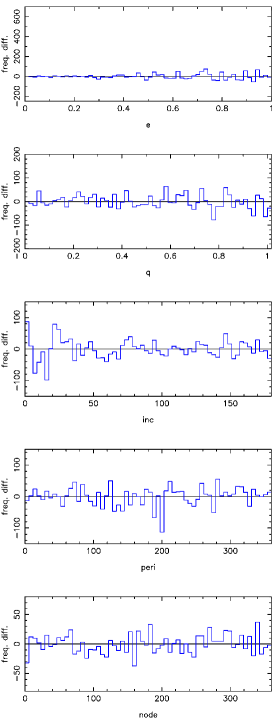
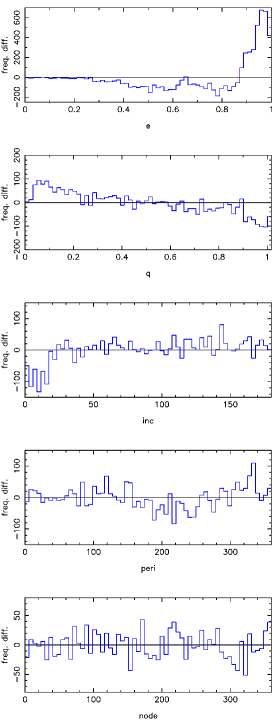
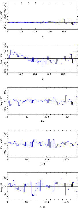
Figure 4: Plot of the differences of the absolute frequencies of the marginal distributions of orbital elements of the observed and synthetic data. From the left, in the columns we have the differences between CAMSA and CAMSB data, between CAMSA and KDns data, and between CAMSA and ME4 data. Positive values indicate the prevalence of frequencies in a given bin for CAMSA data.

In Fig. 4 we plotted the differences of frequencies corresponding to the same bins of the histograms of marginal distributions of the orbital elements. The left column illustrates the differences between the CAMSA and CAMSB subsamples, the remaining columns show the differences between the CAMSA and KDns and CAMSA and ME4 samples. Except for a few cases, the differences are essentially equivalent to each other. However, the KDns method does not cope with generating orbits with large eccentricities. Similar problems arise for small and large perihelion distances, and for small inclinations. In case of the ME4 method, the same problems arise for small and large perihelion distances. The reference differences between CAMSA and CAMSB data are clearly random. This cannot be said for the differences in eccentricity, perihelion distance, and partly in inclination for the KDns sample. However, also for the ME4 method, the systematic trend is evident for the perihelion distance. Taking into account the results of the $\chi^{2}$-tests from Table LABEL:tab:chi-KS1 and the course of differences in Fig. 4, in our opinion, the ME4 method gives more consistent results than the KDns method.

One-dimensional K-S tests

Use of binned data involves a loss of information, however. Additionally, there is often considerable arbitrariness as to how the bins should be chosen. The results given in the first section of Table LABEL:tab:chi-KS1 were obtained assuming the following ranges for the observed and synthetic orbital elements: $e\in[0,1)$, $q\in[0,1.068)$, $i\in[0.180)$, $\omega\in[0,360)$ and $\Omega\in[0,360)$. For each orbital element, these intervals were divided by $62$, and the number of bins was calculated by the Rice Rule.

To avoid the problem of the influence of the number of bins, we applied the K-S test to the unbinned data of $e,q,\omega,\Omega,i$ orbital elements. We used the 1D K-S test, and more particularly, we used the kstwo subroutine taken from the ‘Numerical Recipes’ package (Press et al., 2002). The results of the K-S tests are given in the second section of Table LABEL:tab:chi-KS1. Like the earlier $\chi^{2}$ tests, the 1D K-S test for $q$ gave negative results for all synthetic samples. Furthermore, like the previous test the K-S test shows that the ME methods give results closer to the observed sample than the KD methods.

Two-dimensional tests

We describe the results of a comparison of the observed and synthetic samples applying the $\chi^{2}$-distance (Eq. (1)) and a two-dimensional K-S test for all pairs of orbital elements. The 2D K-S test was performed using the ks2d2s subroutine taken from the ‘Numerical Recipes’ package (Press et al., 2002). Results are provided in Table LABEL:tab:chi-KS2. The first section of Table LABEL:tab:chi-KS2 provides the $\chi^{2}$ distances between the observed CAMSA and the synthetic KD10, KDns, ME0, ME1, and ME4 samples. The results for the observed CAMSB data are for reference. As we can see, on the basis of this table, it is impossible to establish which method gives the best orbits. The result depends on what pair of orbital elements we choose. Choosing the pair $q$-$\omega$, the ME4 method gives the result closest to the observed sample. Choosing $q$-$e$, KDns is the best. Choosing the pair $q$-$i$ we see that for the KDns the $\chi^{2}$ distance is smaller than for the reference CAMSB sample, and this indicates that KDns gives orbits that are too similar to the observed sample. Hence, for the pair $q$-$i$, the KD10 method takes precedence. The same is true for the pair $q$-$\Omega$, therefore the ME4 method takes precedence. In the case of KDns method, for five orbital element pairs, the $\chi^{2}$ distances prove to be smaller than for the CAMSB data, for the KD10 method three times, respectively. On the other hand, this was not the case with all ME methods.

The results of the 2D K-S tests for all pairs of orbital elements are given in the second section of Table LABEL:tab:chi-KS2. As one can see, in general the results of these tests are negative for all methods. Some exceptions are the results obtained for the pair $e$-$\Omega$ and ME0 and ME1 methods.

Table 4: Distances of $\chi^{2}$ (first section) and results of 2D K-S tests (second section) for the pairs of orbital elements. The orbits from the CAMSA sample were compared with orbits generated using the KD10, KDns, ME0, ME1, and ME4 methods. The results of a comparison of the CAMSA and CAMSB samples serve as a reference for the other tests. In the first section of the table, in each row we indicate the values, the most (red) and least (green), differing from the result corresponding to the reference sample.

	CAMSB	KD10	KDns	ME0	ME1	ME4
q-$\omega$	751	6287	3010	7360	5512	1743
q-e	1193	2319	2148	4377	3599	2566
q-i	1820	1996	1515	4028	3269	2755
q-$\Omega$	1915	2229	1120	3560	2863	1989
e-$\omega$	1522	2352	2277	2642	2670	2656
e-i	1402	2115	2191	2517	2554	2586
e-$\Omega$	1510	1969	2018	1585	1527	1521
$\omega$-$\Omega$	1890	1636	1551	2531	2483	2477
$\omega$-i	1803	1789	1732	3102	3176	3101
i-$\Omega$	1992	1623	1617	2062	2088	2082
	CAMSB	KD10	KDns	ME0	ME1	ME4
q-$\omega$	46.9	0.0	0.0	0.0	0.0	0.0
q-e	48.4	0.0	0.0	0.0	0.0	0.0
q-i	38.7	0.0	0.0	0.0	0.0	0.0
q-$\Omega$	23.8	0.0	0.0	0.0	0.0	0.0
e-$\omega$	31.9	0.0	0.0	0.0	0.0	0.0
e-i	60.0	0.0	0.0	0.0	0.0	0.0
e-$\Omega$	60.0	0.0	0.0	26.9	18.1	4.9
$\omega$-$\Omega$	34.0	0.1	1.6	0.0	0.0	0.0
$\omega$-i	25.7	0.0	0.0	0.0	0.0	0.0
i-$\Omega$	46.9	0.0	0.1	0.2	0.0	0.0

To sum up, it follows that assessing the quality of the synthetic orbit generator only on the basis of comparing boundary distributions can be problematic. Therefore, in the next section we describe the results of further tests based on ${NN_{N}}$ and $H_{N}$ statistics.

4.3.2 Application of ${NN_{N}}$ and $H_{N}$ statistics

To compare the synthetic orbit generators, we also set the values of statistics ${NN_{N}}$ and $H_{N}$. We used formulas (2) and (3) and three D-functions, $D_{SH},D_{H}$, and $\rho_{1}$ described in Southworth & Hawkins (1963), Jopek (1993), and Kholshevnikov et al. (2016) respectively. In the previous tests, we used the marginal 1D or 2D distributions of the observed and synthetic samples. Using ${NN_{N}}$ and $H_{N}$ statistics is a different approach, because to calculate them we have to use all orbital elements simultaneously. The results obtained are given in Table LABEL:tab:DNN_HN.

Table 5: Values of the ${NN_{N}}$ and $H_{N}$ statistics calculated for the observed CAMSA and CAMSB samples, and for the orbits generated by the KD10, KDns, ME0, ME1, and ME4 methods. The results for the CAMSA and CAMSB samples serve as a reference. The $D_{SH}$, $D_{H}$, and $\rho_{1}$ functions were used in the calculations. In each column, we indicate the values, the most (red) and least (green), differing from the results corresponding to the reference samples.

	$NN_{N}$			$H_{N}$
Sample	$D_{SH}$	$D_{H}$	$\rho_{1}$	$D_{SH}$	$D_{H}$	$\rho_{1}$
CAMSA	0.097	0.098	0.106	9.077	9.087	9.161
CAMSB	0.097	0.098	0.106	9.076	9.086	9.161
KD10	0.103	0.102	0.109	9.170	9.150	9.224
KDns	0.097	0.096	0.104	9.098	9.090	9.172
ME0	0.120	0.124	0.125	9.308	9.332	9.356
ME1	0.120	0.124	0.126	9.320	9.338	9.365
ME4	0.113	0.114	0.121	9.245	9.243	9.324

This time, the values of ${NN_{N}}$ and $H_{N}$ for the KD methods proved to be closer to the values for the observed samples than for the ME methods. The KDns gave the closest values for all D-functions, the ME4 method gave the closest values among the ME methods. The values of ${NN_{N}}$ and $H_{N}$ depend on the D-function used in the calculations, which is understandable because these functions are not mutually equivalent. For the $\rho_{1}$ function, the results were always greater than for the remaining ones. For the $D_{SH}$ and $D_{H}$ functions, the results are similar to each other, but in general for the former they are slightly smaller.

It might seem that both statistics are equivalent to each other and differ only by a scaling factor. In general, however, this is not the case, and this can be seen when comparing the $NN_{N}$ and $H_{N}$ values calculated for the CAMSB and KDn1 samples. For the $D_{SH}$ function, the $NN_{N}$ values for both these samples equal $0.097$, while for the $H_{N}$ they are $9.076$ and $9.098$, respectively. A similar situation occurs when we compare the results obtained using the $D_{H}$ function for the same CAMSB and KDns samples. The $NN_{N}$ statistics are $0.098$ and $0.096$ and $H_{N}$ are $9.086$ and $9.090$. The mean neighbor distance $NN_{N}$ for the CAMSB sample may be smaller or greater than for a given KDns sample, while the entropy of CAMSB sample may be smaller or greater than for the same KDns sample.

It should be recalled that these statistics differ in their interpretation; only the $H_{n}$ is a measure of the entropy of a data set, which in our opinion gives the $H_{N}$ statistics an important advantage over $NN_{N}$.

4.3.3 Comparison in practical application

Both ${NN_{N}}$ and $H_{N}$ statistics are the point estimators, hence by using them the assessment of the quality of the generators may only be very general. We believe that a more valuable estimate of the usefulness of synthetic orbit generators can be obtained by comparing the results obtained in a specific practical application. In this section, we present the results of calculations of the thresholds of the orbital similarity, which are key parameters of each cluster analysis. For the orbits generated by KD and ME methods, the thresholds were determined by the numerical experiment as described in Jopek (2020). Applying a single linkage cluster analysis algorithm, the thresholds were found for each meteoroid group of $M$=$2,3,...20$ members, and for each of the $D_{SH}$, $D_{H}$, and $\rho_{1}$ distance functions. All obtained results corresponded to a low probability (less than 1%) of chance clustering. The final individual thresholds $D_{M}$, $M$=$2,3,...20$ were calculated as the arithmetic means of the $D_{M}$ values determined in each of the one hundred orbital samples. The final values are given in Table LABEL:tab:thresholds and their graphical illustration is shown in Fig. 5.

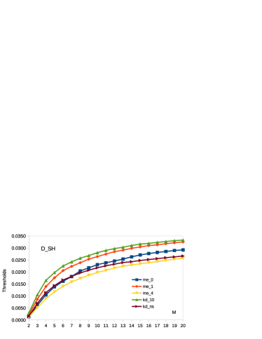
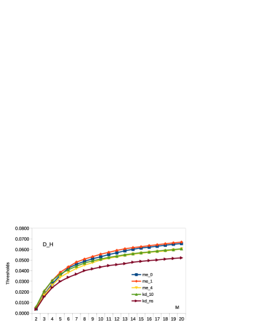
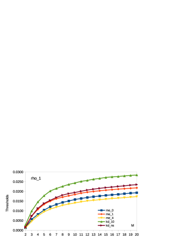
Figure 5: Orbital similarity thresholds calculated for synthetic samples ME0, ME1, ME4, KD10, and KDns, using the $D_{SH},D_{H}$, and $\rho_{1}$ functions. The thresholds were determined for groups of $M$=$2,3,...,20$ members, identified among $29014$ orbits.

Table 6: Values of the orbital similarity thresholds calculated for the synthetic samples obtained by KD and ME methods. The thresholds correspond to each group of $M$=$2,3,...20$ members and for each distance function $D_{SH},D_{H}$, and $\rho_{1}$. The provided values are closely related to the single-linkage cluster analysis method and the size of the synthetic samples used. In this study, we used 29014 orbits.

	M	ME0	ME1	ME4	KD10	KDns
	2	0.0013	0.0022	0.0012	0.0029	0.0015
	3	0.0061	0.0086	0.0051	0.0105	0.0069
	4	0.0105	0.0139	0.0089	0.0165	0.0114
	5	0.0138	0.0176	0.0117	0.0198	0.0143
	6	0.0161	0.0206	0.0140	0.0225	0.0166
	7	0.0181	0.0223	0.0158	0.0242	0.0181
	8	0.0204	0.0238	0.0173	0.0257	0.0196
	9	0.0217	0.0253	0.0186	0.0268	0.0207
	10	0.0230	0.0264	0.0198	0.0280	0.0217
$D_{SH}$	11	0.0238	0.0274	0.0207	0.0290	0.0226
	12	0.0246	0.0284	0.0216	0.0297	0.0233
	13	0.0254	0.0291	0.0224	0.0303	0.0239
	14	0.0263	0.0298	0.0229	0.0310	0.0243
	15	0.0271	0.0304	0.0234	0.0316	0.0248
	16	0.0277	0.0310	0.0239	0.0319	0.0252
	17	0.0281	0.0313	0.0243	0.0323	0.0255
	18	0.0285	0.0318	0.0248	0.0327	0.0259
	19	0.0289	0.0322	0.0253	0.0330	0.0263
	20	0.0292	0.0325	0.0257	0.0333	0.0266
	2	0.0039	0.0056	0.0037	0.0060	0.0036
	3	0.0174	0.0204	0.0169	0.0209	0.0154
	4	0.0277	0.0306	0.0263	0.0307	0.0240
	5	0.0357	0.0385	0.0339	0.0369	0.0299
	6	0.0425	0.0435	0.0383	0.0409	0.0337
	7	0.0460	0.0481	0.0422	0.0442	0.0368
	8	0.0488	0.0509	0.0452	0.0472	0.0401
	9	0.0513	0.0532	0.0476	0.0493	0.0417
	10	0.0531	0.0555	0.0501	0.0509	0.0434
$D_{H}$	11	0.0552	0.0573	0.0517	0.0525	0.0448
	12	0.0569	0.0591	0.0531	0.0537	0.0457
	13	0.0588	0.0606	0.0544	0.0550	0.0467
	14	0.0602	0.0617	0.0555	0.0560	0.0480
	15	0.0614	0.0625	0.0564	0.0569	0.0488
	16	0.0622	0.0636	0.0574	0.0576	0.0495
	17	0.0630	0.0644	0.0580	0.0585	0.0501
	18	0.0640	0.0654	0.0586	0.0592	0.0509
	19	0.0649	0.0662	0.0595	0.0598	0.0515
	20	0.0656	0.0669	0.0604	0.0606	0.0521
	2	0.0012	0.0020	0.0012	0.0028	0.0015
	3	0.0056	0.0073	0.0046	0.0099	0.0073
	4	0.0081	0.0107	0.0073	0.0145	0.0113
	5	0.0103	0.0133	0.0095	0.0178	0.0138
	6	0.0121	0.0149	0.0108	0.0202	0.0154
	7	0.0133	0.0162	0.0119	0.0215	0.0169
	8	0.0143	0.0170	0.0128	0.0225	0.0180
	9	0.0150	0.0177	0.0135	0.0235	0.0189
	10	0.0158	0.0184	0.0140	0.0243	0.0194
$\rho_{1}$	11	0.0163	0.0191	0.0146	0.0251	0.0200
	12	0.0168	0.0196	0.0151	0.0256	0.0207
	13	0.0172	0.0199	0.0154	0.0262	0.0211
	14	0.0176	0.0203	0.0157	0.0266	0.0215
	15	0.0179	0.0206	0.0160	0.0271	0.0219
	16	0.0182	0.0209	0.0163	0.0274	0.0222
	17	0.0184	0.0211	0.0165	0.0276	0.0225
	18	0.0188	0.0213	0.0168	0.0279	0.0228
	19	0.0191	0.0216	0.0170	0.0282	0.0232
	20	0.0193	0.0218	0.0173	0.0284	0.0235

For obvious reasons, we could not compare the results obtained for the synthetic orbits with the thresholds calculated for the observed orbits, hence, our comparisons relate only to synthetic orbits. As expected, the threshold values proved to depend on the applied D-functions and the synthetic data set. Although in all cases the thresholds increased monotonically with the size $M$ of the identified group, this dependency is quite diverse. In Fig. 5 we see that in the case of the $D_{SH}$ function the highest thresholds are for the KD10 orbits, the smallest one for the ME4 orbits. This means that if we use the $D_{SH}$ function and the KD10 orbits in the cluster analysis, then by using the obtained thresholds in the sample of observed orbits, some of the results may turn out to be artifacts, both for the number of identified streams and the number of their members. Using the ME4 orbits, we can face the opposite situation, we cannot identify certain streams, and the number of members of the identified streams may be significantly smaller.

When the $D_{H}$ function is applied, the smallest thresholds are for the KDns orbits, the highest for the ME1 orbits. Finally, in the case of the $\rho_{1}$ function, again, the smallest values are for the ME4 orbits, the highest for the KD10 orbits.

However, we cannot claim that any of the calculated threshold values are too large or too small. That is because we cannot compare the results obtained for the synthetic and observed orbits here. We can only claim that in the case of cluster analysis, among the CAMS orbits (using a single linkage algorithm and $D_{SH}$ or $\rho_{1}$ function), the values of the orbital similarity thresholds will be the smallest if we generate synthetic orbits using the ME4 method. If we apply the $D_{H}$ function, the smallest thresholds will be obtained using the KDns method. Moreover, we cannot be sure that what has been said above would also be true for the observed orbits taken from another source or if another cluster analysis were applied.

5 Conclusions

We compared five methods for generating synthetic meteoroid orbits. Three of them (ME0, KD10, and KDns) had already been proposed in the literature, two additional methods (ME1 and ME4) are new. As far as possible, the synthetic orbits were compared with the orbits obtained as a result of observations, otherwise, the comparison is of a relative nature. For quantitative comparison, we applied a few tests: the $\chi^{2}$-distance and $NN_{N}$ tests used in Vida et al. (2017), and, implemented in this study, one-dimensional $\chi^{2}$ and K-S tests, as well as a two-dimensional K-S test. In addition to the $NN_{N}$ statistics, to estimate a general property of the orbital sample, we used the entropy $H_{N}$ of the data set based on nearest neighbor distances. Finally, we did a cluster analysis among the synthetic orbits. We calculated and compared the values of the orbital similarity thresholds.

As a result of our research, we can make a few conclusions summarized by the following points:

1. Using the $\chi^{2}$ distance (see Eq. (1)) for one pair of orbital elements only, for example, $\omega$-$q$, it is not sufficient to decide which synthetic sample more adequately represents the observed data. It may be risky, as we see in Table LABEL:tab:chi-KS2. The result of the comparison clearly depends on the pair used in the test.

2. The same can be said about the $\chi^{2}$ and K-S tests performed for the marginal distributions of each orbital element. You cannot judge the quality of the orbit generator by only testing the data for a single orbit element (see Table LABEL:tab:chi-KS1). Nevertheless, in our study, the ME methods performed significantly better in the 1D tests than the KD methods.

3. The 2D Kolmogorov-Smirnov test gave negative results for all compared ME and KD methods. In our opinion, it follows that the algorithms of the tested methods are not capable of generating ’realistic’ meteoroid orbits.

4. The $NN_{N}$ and $H_{N}$ statistics gave a clear result. The values of $NN_{N}$ and $H_{N}$ for the orbits obtained by KD10 and KDns are closer to $NN_{N}$ and $H_{N}$ values calculated for the observed orbits. Both statistics are based on nearest neighbor distances, but only the $H_{N}$ statistics is the entropy of a data set.

5. The results of the cluster analysis among synthetic orbits turned out to be dependent on the applied D-function of orbital similarity. For $D_{SH}$ and $\rho_{1}$ functions, the smallest threshold values were obtained for the ME4 method. In the case of $D_{H}$ function, the smallest values were obtained for KDns orbits. By the relative comparison, we cannot decide which orbits give the thresholds as too large or which as too small.

.

The results showed us that the generation of ’realistic’ meteoroid orbits is a complex issue. All methods are based on the observed data, which are heavily biased by observational selection, responsible for a number of correlations between the orbital elements. Including these correlations in an algorithm of a given method is not an easy matter. As far as we know, these correlations are not yet well understood. Perhaps an improvement in the situation can be achieved by using the geocentric parameters of the observed meteoroids (see Froeschlé et al. (1999), Valsecchi et al. (1999)).

The same can be said about the tests and comparisons made in our study. This is also a complex issue. They give very limited results depending on the type of the test, the orbital elements used, the D-function applied, and other factors.

However, we were pleasantly surprised that, in the case of comparisons based on the determination of the thresholds of the orbital similarity, the results obtained, albeit different, were quite similar. Thus, at least in the case of the single linkage cluster analysis, we think that all ME and KD methods can be applied successfully.

Appendix A Generation of the synthetic orbits

A.1 ME methods

ME0
The algorithm of the ME0 method (in Jopek & Bronikowska 2017, it was named ME) involves the following steps:

1. For a given observed sample, obtain the histograms of the orbital elements and additionally find the fraction of the orbits $\beta_{fr}$ for which the geocentric ecliptic latitudes of the meteor radiant $\beta_{G}>0$.

2. Generate $e,\omega,\Omega,i$ separately by the CPD inversion method, (Zieliński 1979).

3. Using the Earth crossing condition (4) with $R_{E}=1$ and the obtained $e,\omega$ calculate $q_{c}$; choose the sign at the $e\cos\omega$ by generating the number $b$ distributed uniformly, $U(0,1)$; if $b>\beta_{fr}$ , choose sign “$-$” otherwise choose sign “$+$”.

4. Using $q_{c}$ and the $e$ generated earlier, calculate the inverse of the semi-major axis $1/a_{c}$, if $1/a_{c}>(1/a)_{max}$, repeat steps (2), (3), (4). ( The inverse $(1/a)_{max}$ is the maximal value in the observed orbital sample).

ME1
This method is based on the ME0, however we incorporated a suggestion given in Vida et al. (2017), which was to set in formula (4), the distance $R_{E}$ depending on the ecliptic longitude $\lambda_{E}$ of the Earth at the moment of time of the meteor appearance. Both $\lambda_{E}$ and $R_{E}$ values were calculated by means of the formulas taken from Bell & Urban (2012). Figure 6 shows that dependence $R_{E}$=$f(\lambda_{E})$ is not random, therefore we applied its approximation

$$R_{E}=0.016710*\sin(\lambda_{E}-192.211073)+1.$$ (7)

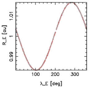
Figure 6: Dependence of the heliocentric distance $R_{E}$ of Earth on the ecliptic longitude $\lambda_{E}$ of Earth at the time of meteor observation. Both values correspond to the meteoroids taken from the CAMSA orbital sample.

Also we have modified the condition for $q_{c}$ and $(1/a)_{c}$. The calculated values had to fulfill the condition

$$q_{min}\leq q_{c}\leq q_{max},$$

$$(1/a)_{min}\leq(1/a)_{c}\leq(1/a)_{max},$$ (8)

where $q_{min},q_{max},(1/a)_{min}$, $(1/a)_{max}$ are given by formula (6).
The algorithm of the ME1 method involves the following steps:

1. For a given observed sample, obtain the histograms of $q,e,\omega,\Omega,i,\lambda_{E},\beta_{G}$.

2. Generate $\beta_{G},\lambda_{E},e,\omega,\Omega,i$ separately by the CPD inversion method.

3. Calculate $R_{E}$ using formula (7).

4. Using the Earth crossing condition (4) and obtained $R_{E},e,\omega$ calculate $q_{c}$; choose the sign at the $e\cos\omega$, if $\beta_{G}>0$ choose sign “$-$” , otherwise choose sign “$+$”,

5. Using $q_{c}$ and the $e$ generated earlier, calculate the inverse of the semi-major axis $1/a_{c}$.

6. If $1/a_{c}$ is outside the interval $[(1/a)_{min},(1/a)_{max}]$ or if $q_{c}$ is outside the interval $[q_{min},q_{max}]$, repeat steps 2, 3, 4.

ME4
The ME4 method is based on the ME1, however with one modification. We made use of the asymmetry of the $\beta_{G}$-$\omega$ distribution (see Fig. 7). Choosing the value $\beta_{G}=0$, the $\omega$ values were divided into two subsamples for which $\beta_{G}\geq 0$ and $\beta_{G}<0$. In the method ME4, instead of the $\omega$-histogram for the whole CAMSA sample we used two histograms corresponding to $\beta_{G}\geq 0$ and $\beta_{G}<0$, respectively. This solution significantly improved the test results obtained with the ME4 method. We can see this if, for example, we compare the values for ME1 and ME4 in the first row of Table LABEL:tab:chi-KS2.

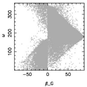
Figure 7: Distribution of $29014$ sporadic CAMSA video meteoroids on the $\beta_{G}$-$\omega$ plane. As can be seen, this plot is asymmetric due to the $\beta_{G}$ coordinate.

Thus, the algorithm of the ME4 method involves the same steps as for the method ME1, except that the argument of perihelion $\omega$ was generated by the CPD inversion method using two $\omega$-histograms, depending on the sign of the generated $\beta_{G}$ value.

A.2 KD methods

The KD methods proposed in Vida et al. (2017) for the generation of synthetic meteoroid orbits make use of the nonparametric technique. It is based on the multivariate kernel density estimation, a function which for the five dimensional problem is given as

$$\hat{f}({O})=\frac{1}{N|{H}|}\sum_{k=1}^{N}K_{5}\left[{H}^{-1}({O}-{O}_{k})\right],$$ (9)

where ${O}$=$(q,e,\omega,\Omega,i)^{T}$, ${O}_{k}$=$(q_{k},e_{k},\omega_{k},\Omega_{k},i_{k})^{T}$, $k$=$1,2,...,N$, and $N$ is the size the orbital sample. The letter ${H}$ represents the bandwidth (or smoothing) $5x5$ matrix; $K_{5}$ is the kernel function, symmetric multivariate density function. In Vida et al. (2017) the authors used a Gaussian kernel. The choice of the kernel function $K$ is not critical to the accuracy of kernel density estimators. The most important factor affecting results obtained by Eq. (9) is the choice of the bandwidth matrix ${H}$. Vida et al. (2017) presented the results of three KD variations. In the KD10 or KD0.1 method the bandwidth $H$ was a scalar matrix with all diagonal elements equal to $10$ or $0.1$, respectively. In the KD non-scalar method (KDns) the bandwidth matrix is defined as

$$\mathbf{H}=\left[\begin{array}[]{ccccc}0.01&0.0&0.0&0.0&0.0\\ 0.0&10&0.0&0.0&0.0\\ 0.0&0.0&10&0.0&0.0\\ 0.0&0.0&0.0&10&0.0\\ 0.0&0.0&0.0&0.0&6\\ \end{array}\right],$$ (10)

where the values on the diagonal correspond to $q,\Omega,e,\omega,i$ respectively. Having the multivariate estimate (9), it can be used to draw a synthetic sample of the orbits, for details see Vida et al. (2017).