Efficient Discovery of Approximate Order Dependencies

Abstract.

Order dependencies (ODs) capture relationships between ordered domains of attributes. Approximate ODs (AODs) capture such relationships even when there exist exceptions in the data. During automated discovery of ODs, validation is the process of verifying whether an OD holds. We present an algorithm for validating approximate ODs with significantly improved runtime performance over existing methods for AODs, and prove that it is correct and has optimal runtime. By replacing the validation step in a leading algorithm for approximate OD discovery with ours, we achieve orders-of-magnitude improvements in performance.

1. Introduction

1.1. Motivation

Functional dependencies (FDs) specify that the values of given attributes functionally determine the value of a target attribute. Order dependencies extend FDs to state that, additionally, the order of tuples with respect to the values from the domains of given attributes determines the order of the values from the domain of the target attribute. Table 1 shows a dataset with employee salaries. In this table, the OD that $\sf{sal}$ orders $\sf{taxGrp}$ holds. If one sorts the table by $\sf{sal}$, it is sorted by $\sf{taxGrp}$ as well.

An OD implies the corresponding FD; e.g., that $\sf{sal}$ orders $\sf{taxGrp}$ implies that $\sf{sal}$ functionally determines $\sf{taxGrp}$. Order compatibility (OC) captures the co-ordering aspect of an OD without the corresponding FD. Any OD can be equivalently represented by a pair of an OC and an FD (Szlichta et al., 2012). In Table 1, that $\sf{taxGrp}$ is order compatible with $\sf{sal}$ holds as there exists an order of the tuples such that they are sorted both by $\sf{taxGrp}$ and by $\sf{sal}$. Note that $\sf{taxGrp}$ does not order $\sf{sal}$ as an FD does not hold.

There has been recent work to automate the discovery of ODs from data (Szlichta et al., 2017, 2018; Consonni et al., 2019; Jin et al., 2020; Langer and Naumann, 2016). In practice, however, such constraints rarely hold perfectly in the data. Real data are dirty, containing wrong and inconsistent values that may violate semantically valid dependencies. This motivates the need for discovering approximate ODs (AODs), ODs that hold in the data but with exceptions. Discovered ODs deemed semantically valid can be used for data cleaning, to detect erroneous tuples, where measures are then taken to repair the errors (Qiu et al., 2018). Approximate ODs are useful even when the data are not dirty, as there can be exceptions to general rules. AODs help avoid overfitting by discovering more general and meaningful dependencies.

In Table 1, tax is a fixed percentage of salary in each tax group; i.e., one, three, or eight percent. However, $\sf{perc}$ includes a concatenated zero in some rows due to data entry errors (e.g., 10% instead of 1% in ${\mathchoice{\mbox{\sf t}}{\mbox{\sf t}}{\mbox{\scriptsize\sf t}}{\mbox{\tiny\sf t}}}_{1}$). Because of this, the OC that $\sf{salary}$ is order compatible with $\sf{tax}$ does not hold, even though this OC is intended. Similarly, the FD that $\sf{pos}$, $\sf{exp}$ functionally determines $\sf{sal}$ does not hold, due to the exception of tuples ${\mathchoice{\mbox{\sf t}}{\mbox{\sf t}}{\mbox{\scriptsize\sf t}}{\mbox{\tiny\sf t}}}_{6}$ and ${\mathchoice{\mbox{\sf t}}{\mbox{\sf t}}{\mbox{\scriptsize\sf t}}{\mbox{\tiny\sf t}}}_{7}$, two employees with the same position and years of experience but having different salaries. With approximate ODs, we can still discover such concise and meaningful rules in these instances.

Table 1. Employee salaries

$\sf{\#}$	$\sf{pos}$	$\sf{exp}$	$\sf{sal}$	$\sf{taxGrp}$	$\sf{perc}$	$\sf{tax}$	$\sf{bonus}$
${\mathchoice{\mbox{\sf t}}{\mbox{\sf t}}{\mbox{\scriptsize\sf t}}{\mbox{\tiny\sf t}}}_{1}$	sec	1	20K	A	10%	2K	1K
${\mathchoice{\mbox{\sf t}}{\mbox{\sf t}}{\mbox{\scriptsize\sf t}}{\mbox{\tiny\sf t}}}_{2}$	sec	3	25K	A	10%	2.5K	1K
${\mathchoice{\mbox{\sf t}}{\mbox{\sf t}}{\mbox{\scriptsize\sf t}}{\mbox{\tiny\sf t}}}_{3}$	dev	1	30K	A	1%	0.3K	3K
${\mathchoice{\mbox{\sf t}}{\mbox{\sf t}}{\mbox{\scriptsize\sf t}}{\mbox{\tiny\sf t}}}_{4}$	sec	5	40K	B	30%	12K	2K
${\mathchoice{\mbox{\sf t}}{\mbox{\sf t}}{\mbox{\scriptsize\sf t}}{\mbox{\tiny\sf t}}}_{5}$	dev	3	50K	B	3%	1.5K	4K
${\mathchoice{\mbox{\sf t}}{\mbox{\sf t}}{\mbox{\scriptsize\sf t}}{\mbox{\tiny\sf t}}}_{6}$	dev	5	55K	B	30%	16.5K	4K
${\mathchoice{\mbox{\sf t}}{\mbox{\sf t}}{\mbox{\scriptsize\sf t}}{\mbox{\tiny\sf t}}}_{7}$	dev	5	60K	B	3%	1.8K	4K
${\mathchoice{\mbox{\sf t}}{\mbox{\sf t}}{\mbox{\scriptsize\sf t}}{\mbox{\tiny\sf t}}}_{8}$	dev	-1	90K	C	8%	7.2K	7K
${\mathchoice{\mbox{\sf t}}{\mbox{\sf t}}{\mbox{\scriptsize\sf t}}{\mbox{\tiny\sf t}}}_{9}$	dir	8	200K	C	8%	16K	10K

Approximate canonical ODs were first introduced in (Szlichta et al., 2017). Their definition of AODs, as is ours herein, is based on the concept of “tuple removal.” Given a table and an OD, a removal set is a set of tuples which, if removed from the table, results in the OD holding. A minimal removal set is one with the smallest cardinality. An approximation factor can be defined with respect to a table and an OD, as the ratio of the size of a minimal removal set over the size of the table. For instance, for Table 1 and the OC that $\sf{pos}$, $\sf{exp}$ is order compatible with $\sf{pos}$, $\sf{sal}$, the minimal removal set and the approximation factor are $\{{\mathchoice{\mbox{\sf t}}{\mbox{\sf t}}{\mbox{\scriptsize\sf t}}{\mbox{\tiny\sf t}}}_{8}\}$ and $1/9\approx 0.11$, respectively.

Given a table r and an approximation threshold $0\leq\epsilon\leq 1$, the discovery problem for AODs is to find the complete set of minimal valid AODs in r w.r.t. $\epsilon$. Exact ODs are a special case of AODs with an approximation factor of zero. Given a table r, an OD $\varphi$, and a threshold $\epsilon$, the problem of validating the candidate OD as an AOD involves verifying whether the approximation factor of $\varphi$, denoted by $e(\varphi)$, is less than or equal to $\epsilon$.

1.2. Contributions

The extension for AOD discovery in (Szlichta et al., 2017, 2018), however, is impractical due to its performance. To validate a candidate AOC in the search, they iteratively remove the tuple—or one of the tuples, in the case of a tie—that causes the largest number of violations. This has two weaknesses: the runtime is quadratic in the number of tuples, and it is not guaranteed to find a minimal removal set.

That it is quadratic makes it prohibitively expensive to run on larger datasets. (The validation step for a candidate exact OD has a linear runtime in the number of tuples.) So while the OD discovery algorithm in (Szlichta et al., 2017, 2018) is shown to scale to datasets with millions of tuples, it is infeasible to run their adapted AOC discovery algorithm over even moderately sized datasets. During benchmarking, we found in some discovery runs that more than 99% of the running time is spent on validating AOC candidates.

That it deliberately does not guarantee finding a minimal removal set means that the algorithm may overestimate the approximation factor of an AOC candidate. Thus, true AOCs with respect to the approximation threshold can be eliminated, which means that the AOC discovery algorithm is incomplete (while the exact OD discovery algorithm is complete).

In this paper, we resolve this major bottleneck in AOD discovery via an algorithm with optimal runtime and guaranteed minimal removal set for validating AOC candidates. This brings performance of AOD discovery on par with that of OD discovery while making the AOD discovery complete.

The paper is structured as follows, with the following key contributions. In Section 2, we provide background and discuss related work. In Sec. 3.1 we illustrate the established OD and AOD discovery framework—which we then adapt herein— and, in Sec. 3.2, the iterative validation algorithm (Szlichta et al., 2017, 2018) it employs. In Sec. 3.3, we contribute a minimal and optimal validation algorithm based on longest increasing subsequences that decreases the runtime from quadratic to super-linear. In Sec. 4, we present our experimental results, with the following contributions. We demonstrate that AOD discovery using our validation algorithm scales to datasets with millions of tuples and tens of attributes (Exp-4.1 and Exp-2). We compare our adapted AOC discovery against the previous approach and demonstrate that ours is orders of magnitude faster (Exp-4.2). As discovering AODs enables the application of pruning rules earlier than for discovering ODs, AOD discovery can be just as efficient, if not more so. Our AOD discovery algorithm gains up to 76% improvement in runtime compared against the (exact) OD discovery algorithm (Exp-4.3). Given our AOD discovery algorithm is complete, we discover more AODs, and semantically more general AODs (thus, of higher quality). We show that we find more AODs, both due to our better scalability and the minimality of our removal sets (Exp-4 and Exp-5). In Section 5, we conclude with suggestions for future work. In Section 6, we prove our theorems.

2. Preliminaries and Related Work

2.1. Definitions and Notation

R denotes a relational schema, r represents a table instance, and s and t denote tuples. $\sf{A}$ and $\sf{B}$ denote individual attributes and ${\mathcal{X}}$ and ${\mathcal{Y}}$ sets of attributes. Lists of attributes are presented using X and Y; $[{}]$ denotes the empty list and $[{\sf{A}}\,|\,{{\mathchoice{\mbox{{T}}}{\mbox{{T}}}{\mbox{\scriptsize{T}}}{\mbox{\tiny{T}}}}}]$ denotes a list with head attribute $\sf{A}$ and tail list T. Tuples ${\mathchoice{\mbox{\sf t}}{\mbox{\sf t}}{\mbox{\scriptsize\sf t}}{\mbox{\tiny\sf t}}}_{\sf{A}}$ and ${\mathchoice{\mbox{\sf t}}{\mbox{\sf t}}{\mbox{\scriptsize\sf t}}{\mbox{\tiny\sf t}}}_{{\mathcal{X}}}$ denote the projections of tuple t on $\sf{A}$ and ${\mathcal{X}}$, respectively. Wherever a set is expected but a list appears, the list is cast to a set; e.g., ${\mathchoice{\mbox{\sf t}}{\mbox{\sf t}}{\mbox{\scriptsize\sf t}}{\mbox{\tiny\sf t}}}_{{\mathchoice{\mbox{{X}}}{\mbox{{X}}}{\mbox{\scriptsize{X}}}{\mbox{\tiny{X}}}}}$ is equivalent to ${\mathchoice{\mbox{\sf t}}{\mbox{\sf t}}{\mbox{\scriptsize\sf t}}{\mbox{\tiny\sf t}}}_{{\mathcal{X}}}$. ${\mathchoice{\mbox{{X}}}{\mbox{{X}}}{\mbox{\scriptsize{X}}}{\mbox{\tiny{X}}}}^{\prime}$ represents an arbitrary permutation of the values of a list X or set ${\mathcal{X}}$.

Definition 2.1.

(nested order) Let X be a list of attributes where ${\mathcal{X}}\in{\mathchoice{\mbox{R}}{\mbox{R}}{\mbox{\scriptsize R}}{\mbox{\tiny R}}}$. Given two tuples, s and t, ${\mathchoice{\mbox{\sf s}}{\mbox{\sf s}}{\mbox{\scriptsize\sf s}}{\mbox{\tiny\sf s}}}\mathrel{\preceq}_{{\mathchoice{\mbox{{X}}}{\mbox{{X}}}{\mbox{\scriptsize{X}}}{\mbox{\tiny{X}}}}}{\mathchoice{\mbox{\sf t}}{\mbox{\sf t}}{\mbox{\scriptsize\sf t}}{\mbox{\tiny\sf t}}}$ iff

• ${\mathchoice{\mbox{{X}}}{\mbox{{X}}}{\mbox{\scriptsize{X}}}{\mbox{\tiny{X}}}}=[\,]$; or

• ${\mathchoice{\mbox{{X}}}{\mbox{{X}}}{\mbox{\scriptsize{X}}}{\mbox{\tiny{X}}}}=[{\sf{A}}\,|\,{{\mathchoice{\mbox{{T}}}{\mbox{{T}}}{\mbox{\scriptsize{T}}}{\mbox{\tiny{T}}}}}]$ and ${\mathchoice{\mbox{\sf s}}{\mbox{\sf s}}{\mbox{\scriptsize\sf s}}{\mbox{\tiny\sf s}}}_{\sf{A}}<{\mathchoice{\mbox{\sf t}}{\mbox{\sf t}}{\mbox{\scriptsize\sf t}}{\mbox{\tiny\sf t}}}_{\sf{A}}$; or

• ${\mathchoice{\mbox{{X}}}{\mbox{{X}}}{\mbox{\scriptsize{X}}}{\mbox{\tiny{X}}}}=[{\sf{A}}\,|\,{{\mathchoice{\mbox{{T}}}{\mbox{{T}}}{\mbox{\scriptsize{T}}}{\mbox{\tiny{T}}}}}]$, ${\mathchoice{\mbox{\sf s}}{\mbox{\sf s}}{\mbox{\scriptsize\sf s}}{\mbox{\tiny\sf s}}}_{\sf{A}}={\mathchoice{\mbox{\sf t}}{\mbox{\sf t}}{\mbox{\scriptsize\sf t}}{\mbox{\tiny\sf t}}}_{\sf{A}}$, and ${\mathchoice{\mbox{\sf s}}{\mbox{\sf s}}{\mbox{\scriptsize\sf s}}{\mbox{\tiny\sf s}}}\mathrel{\preceq}_{{\mathchoice{\mbox{{T}}}{\mbox{{T}}}{\mbox{\scriptsize{T}}}{\mbox{\tiny{T}}}}}{\mathchoice{\mbox{\sf t}}{\mbox{\sf t}}{\mbox{\scriptsize\sf t}}{\mbox{\tiny\sf t}}}$.

Let ${\mathchoice{\mbox{\sf s}}{\mbox{\sf s}}{\mbox{\scriptsize\sf s}}{\mbox{\tiny\sf s}}}\mathrel{\prec}_{{\mathchoice{\mbox{{X}}}{\mbox{{X}}}{\mbox{\scriptsize{X}}}{\mbox{\tiny{X}}}}}{\mathchoice{\mbox{\sf t}}{\mbox{\sf t}}{\mbox{\scriptsize\sf t}}{\mbox{\tiny\sf t}}}$ iff ${\mathchoice{\mbox{\sf s}}{\mbox{\sf s}}{\mbox{\scriptsize\sf s}}{\mbox{\tiny\sf s}}}\mathrel{\preceq}_{{\mathchoice{\mbox{{X}}}{\mbox{{X}}}{\mbox{\scriptsize{X}}}{\mbox{\tiny{X}}}}}{\mathchoice{\mbox{\sf t}}{\mbox{\sf t}}{\mbox{\scriptsize\sf t}}{\mbox{\tiny\sf t}}}$ but ${\mathchoice{\mbox{\sf t}}{\mbox{\sf t}}{\mbox{\scriptsize\sf t}}{\mbox{\tiny\sf t}}}\mathrel{\not\preceq}_{{\mathchoice{\mbox{{X}}}{\mbox{{X}}}{\mbox{\scriptsize{X}}}{\mbox{\tiny{X}}}}}{\mathchoice{\mbox{\sf s}}{\mbox{\sf s}}{\mbox{\scriptsize\sf s}}{\mbox{\tiny\sf s}}}$.

Next, we define order dependencies (Szlichta et al., 2012; Szlichta et al., 2017, 2018; Consonni et al., 2019; Jin et al., 2020; Langer and Naumann, 2016).

Definition 2.2.

(order dependency) Let X and Y be lists of attributes where ${\mathcal{X}},{\mathcal{Y}}\subseteq{\mathchoice{\mbox{R}}{\mbox{R}}{\mbox{\scriptsize R}}{\mbox{\tiny R}}}$. ${\mathchoice{\mbox{{X}}}{\mbox{{X}}}{\mbox{\scriptsize{X}}}{\mbox{\tiny{X}}}}\mapsto{\mathchoice{\mbox{{Y}}}{\mbox{{Y}}}{\mbox{\scriptsize{Y}}}{\mbox{\tiny{Y}}}}$ denotes an order dependency, read as X orders Y. Table r satisfies ${\mathchoice{\mbox{{X}}}{\mbox{{X}}}{\mbox{\scriptsize{X}}}{\mbox{\tiny{X}}}}\mapsto{\mathchoice{\mbox{{Y}}}{\mbox{{Y}}}{\mbox{\scriptsize{Y}}}{\mbox{\tiny{Y}}}}$ (${\mathchoice{\mbox{r}}{\mbox{r}}{\mbox{\scriptsize r}}{\mbox{\tiny r}}}\models{\mathchoice{\mbox{{X}}}{\mbox{{X}}}{\mbox{\scriptsize{X}}}{\mbox{\tiny{X}}}}\mapsto{\mathchoice{\mbox{{Y}}}{\mbox{{Y}}}{\mbox{\scriptsize{Y}}}{\mbox{\tiny{Y}}}}$) iff, for all ${\mathchoice{\mbox{\sf s}}{\mbox{\sf s}}{\mbox{\scriptsize\sf s}}{\mbox{\tiny\sf s}}},{\mathchoice{\mbox{\sf t}}{\mbox{\sf t}}{\mbox{\scriptsize\sf t}}{\mbox{\tiny\sf t}}}\in{\mathchoice{\mbox{r}}{\mbox{r}}{\mbox{\scriptsize r}}{\mbox{\tiny r}}}$, ${\mathchoice{\mbox{\sf s}}{\mbox{\sf s}}{\mbox{\scriptsize\sf s}}{\mbox{\tiny\sf s}}}\mathrel{\preceq}_{{\mathchoice{\mbox{{X}}}{\mbox{{X}}}{\mbox{\scriptsize{X}}}{\mbox{\tiny{X}}}}}{\mathchoice{\mbox{\sf t}}{\mbox{\sf t}}{\mbox{\scriptsize\sf t}}{\mbox{\tiny\sf t}}}$ implies ${\mathchoice{\mbox{\sf s}}{\mbox{\sf s}}{\mbox{\scriptsize\sf s}}{\mbox{\tiny\sf s}}}\mathrel{\preceq}_{{\mathchoice{\mbox{{Y}}}{\mbox{{Y}}}{\mbox{\scriptsize{Y}}}{\mbox{\tiny{Y}}}}}{\mathchoice{\mbox{\sf t}}{\mbox{\sf t}}{\mbox{\scriptsize\sf t}}{\mbox{\tiny\sf t}}}$. X and Y are order equivalent (denoted as ${\mathchoice{\mbox{{X}}}{\mbox{{X}}}{\mbox{\scriptsize{X}}}{\mbox{\tiny{X}}}}\leftrightarrow{\mathchoice{\mbox{{Y}}}{\mbox{{Y}}}{\mbox{\scriptsize{Y}}}{\mbox{\tiny{Y}}}}$), iff ${\mathchoice{\mbox{{X}}}{\mbox{{X}}}{\mbox{\scriptsize{X}}}{\mbox{\tiny{X}}}}\mapsto{\mathchoice{\mbox{{Y}}}{\mbox{{Y}}}{\mbox{\scriptsize{Y}}}{\mbox{\tiny{Y}}}}$ and ${\mathchoice{\mbox{{Y}}}{\mbox{{Y}}}{\mbox{\scriptsize{Y}}}{\mbox{\tiny{Y}}}}\mapsto{\mathchoice{\mbox{{X}}}{\mbox{{X}}}{\mbox{\scriptsize{X}}}{\mbox{\tiny{X}}}}$.

Definition 2.3.

(order compatibility) Let X and Y be lists of attributes where ${\mathcal{X}},{\mathcal{Y}}\subseteq{\mathchoice{\mbox{R}}{\mbox{R}}{\mbox{\scriptsize R}}{\mbox{\tiny R}}}$. X and Y are order compatible, denoted as ${\mathchoice{\mbox{{X}}}{\mbox{{X}}}{\mbox{\scriptsize{X}}}{\mbox{\tiny{X}}}}\mathrel{\sim}{\mathchoice{\mbox{{Y}}}{\mbox{{Y}}}{\mbox{\scriptsize{Y}}}{\mbox{\tiny{Y}}}}$, iff ${\mathchoice{\mbox{{XY}}}{\mbox{{XY}}}{\mbox{\scriptsize{XY}}}{\mbox{\tiny{XY}}}}\leftrightarrow{\mathchoice{\mbox{{YX}}}{\mbox{{YX}}}{\mbox{\scriptsize{YX}}}{\mbox{\tiny{YX}}}}$.

The order dependency ${\mathchoice{\mbox{{X}}}{\mbox{{X}}}{\mbox{\scriptsize{X}}}{\mbox{\tiny{X}}}}\mapsto{\mathchoice{\mbox{{Y}}}{\mbox{{Y}}}{\mbox{\scriptsize{Y}}}{\mbox{\tiny{Y}}}}$ means that Y’s values are monotonically non-decreasing with respect to X’s values. Therefore, if one orders the tuples by X, they are also ordered by Y. The order compatibility (OC) ${\mathchoice{\mbox{{X}}}{\mbox{{X}}}{\mbox{\scriptsize{X}}}{\mbox{\tiny{X}}}}\mathrel{\sim}{\mathchoice{\mbox{{Y}}}{\mbox{{Y}}}{\mbox{\scriptsize{Y}}}{\mbox{\tiny{Y}}}}$ means that there exists a total order of the tuples in which they are ordered according to both X and Y.

Example 2.4.

In Table 1, the OD $\sf{sal}\mapsto\sf{taxGrp}$ holds. The OC $\sf{taxGrp}\mathrel{\sim}\sf{sal}$ holds, even though the OD $\sf{taxGrp}\mapsto\sf{sal}$ does not.

ODs have a strong correspondence with OCs and FDs. An OD ${\mathchoice{\mbox{{X}}}{\mbox{{X}}}{\mbox{\scriptsize{X}}}{\mbox{\tiny{X}}}}\mapsto{\mathchoice{\mbox{{Y}}}{\mbox{{Y}}}{\mbox{\scriptsize{Y}}}{\mbox{\tiny{Y}}}}$ holds iff ${\mathchoice{\mbox{{X}}}{\mbox{{X}}}{\mbox{\scriptsize{X}}}{\mbox{\tiny{X}}}}\mathrel{\sim}{\mathchoice{\mbox{{Y}}}{\mbox{{Y}}}{\mbox{\scriptsize{Y}}}{\mbox{\tiny{Y}}}}$ (OC) and ${\mathcal{X}}\rightarrow{\mathcal{Y}}$ (FD) hold. This gives two sources of violations for ODs: swaps and splits (Szlichta et al., 2012).

Definition 2.5.

(swap) A swap with respect to OC ${\mathchoice{\mbox{{X}}}{\mbox{{X}}}{\mbox{\scriptsize{X}}}{\mbox{\tiny{X}}}}\allowbreak\mathrel{\sim}\allowbreak{\mathchoice{\mbox{{Y}}}{\mbox{{Y}}}{\mbox{\scriptsize{Y}}}{\mbox{\tiny{Y}}}}$ is a pair of tuples s and t such that ${\mathchoice{\mbox{\sf s}}{\mbox{\sf s}}{\mbox{\scriptsize\sf s}}{\mbox{\tiny\sf s}}}\prec_{{\mathchoice{\mbox{{X}}}{\mbox{{X}}}{\mbox{\scriptsize{X}}}{\mbox{\tiny{X}}}}}{\mathchoice{\mbox{\sf t}}{\mbox{\sf t}}{\mbox{\scriptsize\sf t}}{\mbox{\tiny\sf t}}}$ but ${\mathchoice{\mbox{\sf t}}{\mbox{\sf t}}{\mbox{\scriptsize\sf t}}{\mbox{\tiny\sf t}}}\prec_{{\mathchoice{\mbox{{Y}}}{\mbox{{Y}}}{\mbox{\scriptsize{Y}}}{\mbox{\tiny{Y}}}}}{\mathchoice{\mbox{\sf s}}{\mbox{\sf s}}{\mbox{\scriptsize\sf s}}{\mbox{\tiny\sf s}}}$.

Definition 2.6.

(split) A split with respect to FD ${\mathcal{X}}\rightarrow{\mathcal{Y}}$ is a pair of tuples s and t such that ${\mathchoice{\mbox{\sf s}}{\mbox{\sf s}}{\mbox{\scriptsize\sf s}}{\mbox{\tiny\sf s}}}_{{\mathcal{X}}}={\mathchoice{\mbox{\sf t}}{\mbox{\sf t}}{\mbox{\scriptsize\sf t}}{\mbox{\tiny\sf t}}}_{{\mathcal{X}}}$ but ${\mathchoice{\mbox{\sf s}}{\mbox{\sf s}}{\mbox{\scriptsize\sf s}}{\mbox{\tiny\sf s}}}_{{\mathcal{Y}}}\neq{\mathchoice{\mbox{\sf t}}{\mbox{\sf t}}{\mbox{\scriptsize\sf t}}{\mbox{\tiny\sf t}}}_{{\mathcal{Y}}}$

Example 2.7.

In Table 1, given the OD $\sf{pos},\sf{exp}\mapsto\sf{pos},\sf{sal}$, tuples ${\mathchoice{\mbox{\sf t}}{\mbox{\sf t}}{\mbox{\scriptsize\sf t}}{\mbox{\tiny\sf t}}}_{7}$ and ${\mathchoice{\mbox{\sf t}}{\mbox{\sf t}}{\mbox{\scriptsize\sf t}}{\mbox{\tiny\sf t}}}_{8}$ constitute a swap (the OC $\sf{pos},\sf{exp}\allowbreak\mathrel{\sim}\allowbreak\sf{pos},\sf{sal}$), and tuples ${\mathchoice{\mbox{\sf t}}{\mbox{\sf t}}{\mbox{\scriptsize\sf t}}{\mbox{\tiny\sf t}}}_{6}$ and ${\mathchoice{\mbox{\sf t}}{\mbox{\sf t}}{\mbox{\scriptsize\sf t}}{\mbox{\tiny\sf t}}}_{7}$ constitute a split (the FD $\sf{pos},\sf{exp}\rightarrow\sf{pos},\sf{sal}$).

Definition 2.8.

tuples s and t are equivalent w.r.t. set of attributes ${\mathcal{X}}$ iff ${\mathchoice{\mbox{\sf{\sf s}}}{\mbox{\sf{\sf s}}}{\mbox{\scriptsize\sf{\sf s}}}{\mbox{\tiny\sf{\sf s}}}}_{{\mathcal{X}}}$ $=$ ${\mathchoice{\mbox{\sf{\sf t}}}{\mbox{\sf{\sf t}}}{\mbox{\scriptsize\sf{\sf t}}}{\mbox{\tiny\sf{\sf t}}}}_{{\mathcal{X}}}$. An attribute set ${\mathcal{X}}$ partitions tuples into equivalence classes (Huhtala et al., 1999). The equivalence class of tuple ${\mathchoice{\mbox{\sf t}}{\mbox{\sf t}}{\mbox{\scriptsize\sf t}}{\mbox{\tiny\sf t}}}\in{\mathchoice{\mbox{r}}{\mbox{r}}{\mbox{\scriptsize r}}{\mbox{\tiny r}}}$ w.r.t. ${\mathcal{X}}$ is denoted by ${\mathcal{E}}({\mathchoice{\mbox{\sf t}}{\mbox{\sf t}}{\mbox{\scriptsize\sf t}}{\mbox{\tiny\sf t}}}_{{\mathcal{X}}})$; i.e., ${\mathcal{E}}({\mathchoice{\mbox{\sf t}}{\mbox{\sf t}}{\mbox{\scriptsize\sf t}}{\mbox{\tiny\sf t}}}_{{\mathcal{X}}})$ = $\{{\mathchoice{\mbox{\sf s}}{\mbox{\sf s}}{\mbox{\scriptsize\sf s}}{\mbox{\tiny\sf s}}}\in{\mathchoice{\mbox{r}}{\mbox{r}}{\mbox{\scriptsize r}}{\mbox{\tiny r}}}\mid{\mathchoice{\mbox{\sf s}}{\mbox{\sf s}}{\mbox{\scriptsize\sf s}}{\mbox{\tiny\sf s}}}_{{\mathcal{X}}}$ = ${\mathchoice{\mbox{\sf t}}{\mbox{\sf t}}{\mbox{\scriptsize\sf t}}{\mbox{\tiny\sf t}}}_{{\mathcal{X}}}\}$. Given a set of attributes ${\mathcal{X}}$, a partition of the table with respect to ${\mathcal{X}}$ is the set of all equivalence classes; i.e., $\Pi_{{\mathcal{X}}}$ = $\{{\mathcal{E}}({\mathchoice{\mbox{\sf t}}{\mbox{\sf t}}{\mbox{\scriptsize\sf t}}{\mbox{\tiny\sf t}}}_{{\mathcal{X}}})$ $|$ ${\mathchoice{\mbox{\sf t}}{\mbox{\sf t}}{\mbox{\scriptsize\sf t}}{\mbox{\tiny\sf t}}}\in{\mathchoice{\mbox{r}}{\mbox{r}}{\mbox{\scriptsize r}}{\mbox{\tiny r}}}\}$.

Example 2.9.

In Table 1, ${\mathcal{E}}({\mathchoice{\mbox{\sf${\mathchoice{\mbox{\sf t}}{\mbox{\sf t}}{\mbox{\scriptsize\sf t}}{\mbox{\tiny\sf t}}}_{1}$}}{\mbox{\sf${\mathchoice{\mbox{\sf t}}{\mbox{\sf t}}{\mbox{\scriptsize\sf t}}{\mbox{\tiny\sf t}}}_{1}$}}{\mbox{\scriptsize\sf${\mathchoice{\mbox{\sf t}}{\mbox{\sf t}}{\mbox{\scriptsize\sf t}}{\mbox{\tiny\sf t}}}_{1}$}}{\mbox{\tiny\sf${\mathchoice{\mbox{\sf t}}{\mbox{\sf t}}{\mbox{\scriptsize\sf t}}{\mbox{\tiny\sf t}}}_{1}$}}}_{{\{\sf{pos}\}}})$ = ${\mathcal{E}}({\mathchoice{\mbox{\sf${\mathchoice{\mbox{\sf t}}{\mbox{\sf t}}{\mbox{\scriptsize\sf t}}{\mbox{\tiny\sf t}}}_{2}$}}{\mbox{\sf${\mathchoice{\mbox{\sf t}}{\mbox{\sf t}}{\mbox{\scriptsize\sf t}}{\mbox{\tiny\sf t}}}_{2}$}}{\mbox{\scriptsize\sf${\mathchoice{\mbox{\sf t}}{\mbox{\sf t}}{\mbox{\scriptsize\sf t}}{\mbox{\tiny\sf t}}}_{2}$}}{\mbox{\tiny\sf${\mathchoice{\mbox{\sf t}}{\mbox{\sf t}}{\mbox{\scriptsize\sf t}}{\mbox{\tiny\sf t}}}_{2}$}}}_{{\{\sf{pos}\}}})$ = ${\mathcal{E}}({\mathchoice{\mbox{\sf${\mathchoice{\mbox{\sf t}}{\mbox{\sf t}}{\mbox{\scriptsize\sf t}}{\mbox{\tiny\sf t}}}_{4}$}}{\mbox{\sf${\mathchoice{\mbox{\sf t}}{\mbox{\sf t}}{\mbox{\scriptsize\sf t}}{\mbox{\tiny\sf t}}}_{4}$}}{\mbox{\scriptsize\sf${\mathchoice{\mbox{\sf t}}{\mbox{\sf t}}{\mbox{\scriptsize\sf t}}{\mbox{\tiny\sf t}}}_{4}$}}{\mbox{\tiny\sf${\mathchoice{\mbox{\sf t}}{\mbox{\sf t}}{\mbox{\scriptsize\sf t}}{\mbox{\tiny\sf t}}}_{4}$}}}_{{\{\sf{pos}\}}})$ = $\{{\mathchoice{\mbox{\sf t}}{\mbox{\sf t}}{\mbox{\scriptsize\sf t}}{\mbox{\tiny\sf t}}}_{1},{\mathchoice{\mbox{\sf t}}{\mbox{\sf t}}{\mbox{\scriptsize\sf t}}{\mbox{\tiny\sf t}}}_{2},{\mathchoice{\mbox{\sf t}}{\mbox{\sf t}}{\mbox{\scriptsize\sf t}}{\mbox{\tiny\sf t}}}_{4}\}$, and $\Pi_{\sf{pos}}$ = $\{\{{\mathchoice{\mbox{\sf t}}{\mbox{\sf t}}{\mbox{\scriptsize\sf t}}{\mbox{\tiny\sf t}}}_{1},{\mathchoice{\mbox{\sf t}}{\mbox{\sf t}}{\mbox{\scriptsize\sf t}}{\mbox{\tiny\sf t}}}_{2},{\mathchoice{\mbox{\sf t}}{\mbox{\sf t}}{\mbox{\scriptsize\sf t}}{\mbox{\tiny\sf t}}}_{4}\},$ $\{{\mathchoice{\mbox{\sf t}}{\mbox{\sf t}}{\mbox{\scriptsize\sf t}}{\mbox{\tiny\sf t}}}_{3},{\mathchoice{\mbox{\sf t}}{\mbox{\sf t}}{\mbox{\scriptsize\sf t}}{\mbox{\tiny\sf t}}}_{5},{\mathchoice{\mbox{\sf t}}{\mbox{\sf t}}{\mbox{\scriptsize\sf t}}{\mbox{\tiny\sf t}}}_{6},{\mathchoice{\mbox{\sf t}}{\mbox{\sf t}}{\mbox{\scriptsize\sf t}}{\mbox{\tiny\sf t}}}_{7},{\mathchoice{\mbox{\sf t}}{\mbox{\sf t}}{\mbox{\scriptsize\sf t}}{\mbox{\tiny\sf t}}}_{8}\},$ $\{{\mathchoice{\mbox{\sf t}}{\mbox{\sf t}}{\mbox{\scriptsize\sf t}}{\mbox{\tiny\sf t}}}_{9}\}\}$.

2.2. A Canonical Mapping

A natural representation of ODs relies on lists of attributes, as in the ORDER BY statement in SQL, where the order of attributes in the list matters; e.g., the OD $\sf{pos},\sf{sal}\mapsto\sf{pos},\sf{exp}$ is different than the OD $\sf{pos},\sf{sal}\mapsto\sf{exp},\sf{pos}$. This is unlike FDs, where the order of attributes does not matter, as with the GROUP BY statement in SQL. Working within this list-based representation, however, has led to discovery frameworks with factorial worst-case runtimes in the number of attributes (Langer and Naumann, 2016). Fortunately, lists are not inherently necessary to express ODs. In (Szlichta et al., 2017, 2018), the authors rely on a polynomial mapping of list-based ODs into a logically equivalent collection of set-based canonical ODs to devise a discovery framework with exponential worst-case runtime in the number of attributes and linear in the number of tuples.

Definition 2.10.

(canonical order compatibility) Given a set of attributes ${\mathcal{X}}$, ${\mathchoice{\mbox{{X}}}{\mbox{{X}}}{\mbox{\scriptsize{X}}}{\mbox{\tiny{X}}}}^{\prime}\sf{A}\mathrel{\sim}{\mathchoice{\mbox{{X}}}{\mbox{{X}}}{\mbox{\scriptsize{X}}}{\mbox{\tiny{X}}}}^{\prime}\sf{B}$ is the OC that states that attributes $\sf{A}$ and $\sf{B}$ are order compatible within each equivalence class of ${\mathcal{X}}$. We write this as ${\mathcal{X}}\mbox{: }\sf{A}\mathrel{\sim}\sf{B}$ in the canonical notation, factoring out the common prefix, and refer to this as a canonical OC.

Definition 2.11.

(order functional dependency) Given a set of attributes ${\mathcal{X}}$, the FD that states that an attribute $\sf{A}$ is constant within each equivalence class of ${\mathcal{X}}$ is equivalent to the list-based OD ${\mathchoice{\mbox{{X}}}{\mbox{{X}}}{\mbox{\scriptsize{X}}}{\mbox{\tiny{X}}}}^{\prime}\mapsto{\mathchoice{\mbox{{X}}}{\mbox{{X}}}{\mbox{\scriptsize{X}}}{\mbox{\tiny{X}}}}^{\prime}\sf{A}$. We write this as ${\mathcal{X}}\mbox{: }[{}]{}\mapsto\sf{A}$ in the canonical notation, and refer to this as an order functional dependency (OFD).

Given a canonical OC of ${\mathcal{X}}\mbox{: }\sf{A}\mathrel{\sim}\sf{B}$ or an OFD of ${\mathcal{X}}\mbox{: }[{}]{}\mapsto\sf{A}$, the set ${\mathcal{X}}$ is referred to as the context of the respective canonical OC or OFD. Intuitively, the context is the common prefix on the left- and right-side of the corresponding list-based OC or OD.

Canonical OCs and OFDs constitute the canonical ODs; i.e., ${\mathchoice{\mbox{{\sf OD}}}{\mbox{{\sf OD}}}{\mbox{\scriptsize{\sf OD}}}{\mbox{\tiny{\sf OD}}}}\equiv{\mathchoice{\mbox{{\sf OC}}}{\mbox{{\sf OC}}}{\mbox{\scriptsize{\sf OC}}}{\mbox{\tiny{\sf OC}}}}+{\mathchoice{\mbox{{\sf OFD}}}{\mbox{{\sf OFD}}}{\mbox{\scriptsize{\sf OFD}}}{\mbox{\tiny{\sf OFD}}}}$. The OD of ${\mathchoice{\mbox{{X}}}{\mbox{{X}}}{\mbox{\scriptsize{X}}}{\mbox{\tiny{X}}}}^{\prime}\sf{A}\mapsto{\mathchoice{\mbox{{X}}}{\mbox{{X}}}{\mbox{\scriptsize{X}}}{\mbox{\tiny{X}}}}^{\prime}\sf{B}$ is logically equivalent to the canonical OC of ${\mathcal{X}}\mbox{: }\sf{A}\mathrel{\sim}\sf{B}$ and OFD of ${\mathcal{X}}\sf{A}\mbox{: }[{}]{}\mapsto\sf{B}$. This is ${\mathcal{X}}\mbox{: }\sf{A}\mapsto\sf{B}$ written in the canonical form.

Example 2.12.

In Table 1, $\sf{sal}$ and $\sf{bonus}$ are order compatible w.r.t. the context $\sf{pos}$; i.e., $\{\sf{pos}\}\mbox{: }\sf{sal}\mathrel{\sim}\sf{bonus}$. In the same table, $\sf{bonus}$ is constant w.r.t. the context $\sf{pos},\sf{sal}$; i.e., $\{\sf{pos},\sf{sal}\}\mbox{: }[{}]{}\mapsto\sf{bonus}$. Therefore, $\sf{sal}$ orders $\sf{bonus}$ w.r.t. the context $\sf{pos}$; i.e., $\{\sf{pos}\}\mbox{: }\sf{sal}\mapsto\sf{bonus}$.

This mapping generalizes: an OD ${\mathchoice{\mbox{{X}}}{\mbox{{X}}}{\mbox{\scriptsize{X}}}{\mbox{\tiny{X}}}}\allowbreak\mathrel{\mapsto}\allowbreak{\mathchoice{\mbox{{Y}}}{\mbox{{Y}}}{\mbox{\scriptsize{Y}}}{\mbox{\tiny{Y}}}}$ holds iff ${\mathchoice{\mbox{{X}}}{\mbox{{X}}}{\mbox{\scriptsize{X}}}{\mbox{\tiny{X}}}}\allowbreak\mathrel{\mapsto}\allowbreak{\mathchoice{\mbox{{X}}}{\mbox{{X}}}{\mbox{\scriptsize{X}}}{\mbox{\tiny{X}}}}{\mathchoice{\mbox{{Y}}}{\mbox{{Y}}}{\mbox{\scriptsize{Y}}}{\mbox{\tiny{Y}}}}$ and ${\mathchoice{\mbox{{X}}}{\mbox{{X}}}{\mbox{\scriptsize{X}}}{\mbox{\tiny{X}}}}\allowbreak\mathrel{\sim}\allowbreak{\mathchoice{\mbox{{Y}}}{\mbox{{Y}}}{\mbox{\scriptsize{Y}}}{\mbox{\tiny{Y}}}}$. These can be encoded into an equivalent set of canonical OFDs and OCs as follows. In the context of ${\mathcal{X}}$, all attributes in ${\mathcal{Y}}$ must be constants. In the context of all prefixes of X and of Y, the trailing attributes must be order compatible:

${\mathchoice{\mbox{R}}{\mbox{R}}{\mbox{\scriptsize R}}{\mbox{\tiny R}}}\models{\mathchoice{\mbox{{X}}}{\mbox{{X}}}{\mbox{\scriptsize{X}}}{\mbox{\tiny{X}}}}\allowbreak\mathrel{\mapsto}\allowbreak{\mathchoice{\mbox{{X}}}{\mbox{{X}}}{\mbox{\scriptsize{X}}}{\mbox{\tiny{X}}}}{\mathchoice{\mbox{{Y}}}{\mbox{{Y}}}{\mbox{\scriptsize{Y}}}{\mbox{\tiny{Y}}}}\mathrel{\emph{iff}}\forall\sf{A}\in{\mathchoice{\mbox{{Y}}}{\mbox{{Y}}}{\mbox{\scriptsize{Y}}}{\mbox{\tiny{Y}}}}.\ {\mathchoice{\mbox{R}}{\mbox{R}}{\mbox{\scriptsize R}}{\mbox{\tiny R}}}\models{\mathcal{X}}\!\mathbin{:}\allowbreak[{}]\allowbreak\mathrel{\mapsto}\allowbreak\sf{A}$ and

${\mathchoice{\mbox{R}}{\mbox{R}}{\mbox{\scriptsize R}}{\mbox{\tiny R}}}\models{\mathchoice{\mbox{{X}}}{\mbox{{X}}}{\mbox{\scriptsize{X}}}{\mbox{\tiny{X}}}}\allowbreak\mathrel{\sim}\allowbreak{\mathchoice{\mbox{{Y}}}{\mbox{{Y}}}{\mbox{\scriptsize{Y}}}{\mbox{\tiny{Y}}}}\mathrel{\emph{iff}}$ $\forall i,j.\ {\mathchoice{\mbox{R}}{\mbox{R}}{\mbox{\scriptsize R}}{\mbox{\tiny R}}}\models[{\sf{X}_{1},\ldots,\sf{X}_{i-1}}][{\sf{Y}_{1},\ldots,\sf{Y}_{j-1}}]\!\mathbin{:}\allowbreak\sf{X}_{i}\allowbreak\mathrel{\sim}\allowbreak\sf{Y}_{j}$.

Thus, list-based ODs can be polynomially mapped to a set of equivalent canonical ODs; i.e., canonical OCs and OFDs (Szlichta et al., 2017, 2018).

Example 2.13.

The OD $[{\sf{A},\sf{B}}]\mapsto[{\sf{C},\sf{D}}]$ is equivalent to the following canonical ODs: $\{\sf{A},\sf{B}\}\mbox{: }[{}]{}\mapsto\sf{C}$, $\{\sf{A},\sf{B}\}\mbox{: }[{}]{}\mapsto\sf{D}$, $\{\}\mbox{: }\sf{A}\mathrel{\sim}\sf{C}$, $\{\sf{A}\}\mbox{: }\sf{B}\mathrel{\sim}\sf{C}$, $\{\sf{C}\}\mbox{: }\sf{A}\mathrel{\sim}\sf{D}$, and $\{\sf{A},\sf{C}\}\mbox{: }\sf{B}\mathrel{\sim}\sf{D}$.

While various algorithms have been proposed for discovering ODs, most are not complete. The algorithm described in (Langer and Naumann, 2016) relies on the list-based definition and employs aggressive pruning rules to compensate for its factorial time complexity, but which make it deliberately incomplete. The authors in (Jin et al., 2020) claim completeness but their algorithm misses ODs in which the same attributes are repeated on the left- and right-hand side. A similar completeness claim has been made in (Consonni et al., 2019), which is shown to be incorrect in (Szlichta et al., 2020). The set-based OD discovery algorithm proposed in (Szlichta et al., 2017) does offer a sound and complete discovery of ODs. We build our algorithm atop the framework introduced in (Szlichta et al., 2017).

In this work, we refer to canonical OCs simply as OCs. As will be discussed in Section 3, we focus on approximate OCs (AOCs), as an efficient algorithm for validating approximate OFDs has already been established (Huhtala et al., 1999). In Section 3.3, we extend our validation algorithm to handle list-based ODs as well.

2.3. Definition of Approximate ODs

We define approximate ODs based upon the fewest tuples that must be removed from a table for an OD to hold. This definition was used for canonical ODs in (Szlichta et al., 2017); their validation step has a quadratic runtime. For approximate FDs, validation is possible in linear time (Huhtala et al., 1999).

Definition 2.14.

Given a table r and an OD $\varphi$, a set of tuples s is a removal set w.r.t. $\varphi$ iff ${\mathchoice{\mbox{r}}{\mbox{r}}{\mbox{\scriptsize r}}{\mbox{\tiny r}}}\setminus{\mathchoice{\mbox{s}}{\mbox{s}}{\mbox{\scriptsize s}}{\mbox{\tiny s}}}\models\varphi$. Let $|{\mathchoice{\mbox{r}}{\mbox{r}}{\mbox{\scriptsize r}}{\mbox{\tiny r}}}|$ denote the cardinality of r, the number of tuples in r. A removal set s is a minimal removal set iff it has the smallest cardinality over all removal sets; i.e., $|{\mathchoice{\mbox{s}}{\mbox{s}}{\mbox{\scriptsize s}}{\mbox{\tiny s}}}|=\min(\{|{\mathchoice{\mbox{s}}{\mbox{s}}{\mbox{\scriptsize s}}{\mbox{\tiny s}}}|\mid{\mathchoice{\mbox{s}}{\mbox{s}}{\mbox{\scriptsize s}}{\mbox{\tiny s}}}\subseteq{\mathchoice{\mbox{r}}{\mbox{r}}{\mbox{\scriptsize r}}{\mbox{\tiny r}}},\ {\mathchoice{\mbox{r}}{\mbox{r}}{\mbox{\scriptsize r}}{\mbox{\tiny r}}}\setminus{\mathchoice{\mbox{s}}{\mbox{s}}{\mbox{\scriptsize s}}{\mbox{\tiny s}}}\models\varphi\})$. Given s, the approximation factor $e(\varphi)$ is defined as $|{\mathchoice{\mbox{s}}{\mbox{s}}{\mbox{\scriptsize s}}{\mbox{\tiny s}}}|/|{\mathchoice{\mbox{r}}{\mbox{r}}{\mbox{\scriptsize r}}{\mbox{\tiny r}}}|$.

Example 2.15.

Consider Table 1 and the OC of $\sf{sal}\mathrel{\sim}\sf{tax}$. Here, ${\mathchoice{\mbox{s}}{\mbox{s}}{\mbox{\scriptsize s}}{\mbox{\tiny s}}}=\{{\mathchoice{\mbox{\sf t}}{\mbox{\sf t}}{\mbox{\scriptsize\sf t}}{\mbox{\tiny\sf t}}}_{1},{\mathchoice{\mbox{\sf t}}{\mbox{\sf t}}{\mbox{\scriptsize\sf t}}{\mbox{\tiny\sf t}}}_{2},{\mathchoice{\mbox{\sf t}}{\mbox{\sf t}}{\mbox{\scriptsize\sf t}}{\mbox{\tiny\sf t}}}_{4},{\mathchoice{\mbox{\sf t}}{\mbox{\sf t}}{\mbox{\scriptsize\sf t}}{\mbox{\tiny\sf t}}}_{6}\}$ and $e(\sf{sal}\mathrel{\sim}\sf{tax})=4/9\approx 0.44$, as ${\mathchoice{\mbox{r}}{\mbox{r}}{\mbox{\scriptsize r}}{\mbox{\tiny r}}}\setminus{\mathchoice{\mbox{s}}{\mbox{s}}{\mbox{\scriptsize s}}{\mbox{\tiny s}}}=\{{\mathchoice{\mbox{\sf t}}{\mbox{\sf t}}{\mbox{\scriptsize\sf t}}{\mbox{\tiny\sf t}}}_{3},{\mathchoice{\mbox{\sf t}}{\mbox{\sf t}}{\mbox{\scriptsize\sf t}}{\mbox{\tiny\sf t}}}_{5},{\mathchoice{\mbox{\sf t}}{\mbox{\sf t}}{\mbox{\scriptsize\sf t}}{\mbox{\tiny\sf t}}}_{7},{\mathchoice{\mbox{\sf t}}{\mbox{\sf t}}{\mbox{\scriptsize\sf t}}{\mbox{\tiny\sf t}}}_{8},{\mathchoice{\mbox{\sf t}}{\mbox{\sf t}}{\mbox{\scriptsize\sf t}}{\mbox{\tiny\sf t}}}_{9}\}$ does not contain any swaps with respect to $\sf{sal}\mathrel{\sim}\sf{tax}$ and no smaller set ${\mathchoice{\mbox{s}}{\mbox{s}}{\mbox{\scriptsize s}}{\mbox{\tiny s}}}^{\prime}$ exists such that ${\mathchoice{\mbox{r}}{\mbox{r}}{\mbox{\scriptsize r}}{\mbox{\tiny r}}}\setminus{\mathchoice{\mbox{s}}{\mbox{s}}{\mbox{\scriptsize s}}{\mbox{\tiny s}}}^{\prime}\models\sf{sal}\mathrel{\sim}\sf{tax}$.

Given a table r and an approximation threshold $\epsilon$, $0\leq\epsilon\leq 1$, the problem of discovering approximate ODs involves finding all minimal (non-redundant that follow from others) ODs $\varphi$ such that $e(\varphi)\leq\epsilon$. In this work, we focus on the problem of validating AOD; i.e., verifying whether the approximation factor of a given AOD is less than or equal to a provided threshold. We present an optimal algorithm for doing so and incorporate it into an existing OD discovery framework.

As discussed in Section 2.2, OCs and OFDs constitute canonical ODs; i.e., ${\mathchoice{\mbox{{\sf OD}}}{\mbox{{\sf OD}}}{\mbox{\scriptsize{\sf OD}}}{\mbox{\tiny{\sf OD}}}}\equiv{\mathchoice{\mbox{{\sf OC}}}{\mbox{{\sf OC}}}{\mbox{\scriptsize{\sf OC}}}{\mbox{\tiny{\sf OC}}}}+{\mathchoice{\mbox{{\sf OFD}}}{\mbox{{\sf OFD}}}{\mbox{\scriptsize{\sf OFD}}}{\mbox{\tiny{\sf OFD}}}}$. There already exists an efficient linear-time algorithm for validating approximate OFDs, as described in (Huhtala et al., 1999). In this work, we present an optimal validation algorithm for AOCs. Note that when discovering approximate OCs and OFDs given an approximation threshold $\epsilon$, ${\mathchoice{\mbox{{\sf OD}}}{\mbox{{\sf OD}}}{\mbox{\scriptsize{\sf OD}}}{\mbox{\tiny{\sf OD}}}}\equiv{\mathchoice{\mbox{{\sf OC}}}{\mbox{{\sf OC}}}{\mbox{\scriptsize{\sf OC}}}{\mbox{\tiny{\sf OC}}}}+{\mathchoice{\mbox{{\sf OFD}}}{\mbox{{\sf OFD}}}{\mbox{\scriptsize{\sf OFD}}}{\mbox{\tiny{\sf OFD}}}}$ does not necessarily hold. If approximate OC ${\mathcal{X}}\mbox{: }\sf{A}\mathrel{\sim}\sf{B}$ and OFD ${\mathcal{X}}\sf{A}\mbox{: }[{}]{}\mapsto\sf{B}$ hold with approximation factors $e_{1},e_{2}\leq\epsilon$, respectively, it is not guaranteed for the corresponding OD of ${\mathcal{X}}\mbox{: }\sf{A}\mapsto\sf{B}$ to also hold approximately with respect to $\epsilon$. As to be discussed in Section 3.3, however, our validation algorithm can easily be extended to validate list-based approximate ODs as well.

3. Discovering Approximate OD’s

In Sec. 3.1, we describe our framework to discover set-based canonical ODs. In Sec. 3.2, we describe the iterative validation algorithm proposed in (Szlichta et al., 2017, 2018), analyze its runtime, and provide an example of it failing to find a minimal removal set and thus overestimating the number of tuples that must be removed. In Sec. 3.3, we present our efficient validation algorithm, based on the longest increasing subsequence (LIS) problem, analyze its runtime, and prove its minimality and optimality.

3.1. Discovery Framework

The algorithm starts the search from singleton sets of attributes and proceeds to traverse the set-based attribute lattice in a level-wise manner (Szlichta et al., 2017, 2018). At each level, and when processing the attribute set ${\mathcal{X}}$, the algorithm verifies OCs of the form ${\mathcal{X}}\setminus\{\sf{A},\sf{B}\}\mbox{: }\sf{A}\mathrel{\sim}\sf{B}$ for which $\sf{A},\sf{B}\in{\mathcal{X}}$ and $\sf{A}\neq\sf{B}$, and OFDs of the form ${\mathcal{X}}\setminus\{\sf{A}\}\mbox{: }[{}]{}\mapsto\sf{A}$ for which $\sf{A}\in{\mathcal{X}}$.

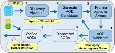
Figure 1. System framework.

Figure 1 illustrates the framework. Candidate AODs are generated based on the attribute sets at the current level of the lattice. Using the dependencies found in previous levels of the lattice, these candidates are then pruned by axioms to avoid redundancy (Szlichta et al., 2017). Our algorithm validates whether each candidate dependency holds approximately, given the approximation threshold as input. Valid AODs are then scored and ranked, using the measure of interestingness introduced in (Szlichta et al., 2017). These discovered AODs can then be manually verified by domain experts, to be then used for tasks such as error repair or outlier detection, which is an easier task than manual specification.

3.2. The Iterative Validation Algorithm

We first discuss the algorithm described in (Szlichta et al., 2017, 2018) to validate an approximate OC given a threshold $\epsilon$. To validate an AOC, the authors propose computing a removal set s by iteratively removing a tuple with the largest number of swaps, which does not guarantee to produce the minimal removal set. This is repeated until either the OC holds or the number of removed tuples crosses the threshold $\epsilon|{\mathchoice{\mbox{r}}{\mbox{r}}{\mbox{\scriptsize r}}{\mbox{\tiny r}}}|$, in which case the AOC candidate is considered invalid. Note that after removing each tuple, the number of swaps for the remaining tuples must be updated.

Algorithm 1 validates a candidate using the iterative approach. The steps in Lines 3 to 15 are repeated on tuples within each equivalence class with respect to the context. Line 4 uses a variant of merge sort to count the number of inversions in the projection of sorted tuples over $\sf{B}$, which is equivalent to the number of swaps for each tuple. Line 7 removes a tuple with the most swaps and Lines 9 to 11 update the number of swaps for the remaining tuples. Line 14 exits if the approximation threshold is crossed.

Algorithm 1 Approx-OC-iterative

Input: Table r, OC ${\mathcal{X}}\mbox{: }\sf{A}\mathrel{\sim}\sf{B}$, and approximation threshold $\epsilon$.                
Output: Approximation factor $e$ and removal set s, or “INVALID”         

1:  ${\mathchoice{\mbox{s}}{\mbox{s}}{\mbox{\scriptsize s}}{\mbox{\tiny s}}}=\{\}$

2:  for all ${\mathcal{E}}\in\Pi_{{\mathcal{X}}}$ do

3:     t $=$ order ${\mathcal{E}}$ by $[\sf{A}$ ASC, $\sf{B}$ ASC$]$

4:     ${\mathchoice{\mbox{\sf{t}}}{\mbox{\sf{t}}}{\mbox{\scriptsize\sf{t}}}{\mbox{\tiny\sf{t}}}}_{\sf{swapCnt}}$ $=$ countInversions$({\mathchoice{\mbox{\sf{t}}}{\mbox{\sf{t}}}{\mbox{\scriptsize\sf{t}}}{\mbox{\tiny\sf{t}}}}_{\sf{B}})$

5:     order t by $\sf{swapCnt}$ ASC

6:     while t is not empty do

7:        ${\mathchoice{\mbox{\sf t}}{\mbox{\sf t}}{\mbox{\scriptsize\sf t}}{\mbox{\tiny\sf t}}}={\mathchoice{\mbox{t}}{\mbox{t}}{\mbox{\scriptsize t}}{\mbox{\tiny t}}}\text{.dropLast()}$

8:        if ${\mathchoice{\mbox{\sf{\sf t}}}{\mbox{\sf{\sf t}}}{\mbox{\scriptsize\sf{\sf t}}}{\mbox{\tiny\sf{\sf t}}}}_{\sf{swapCnt}}\mathrel{==}0$ then break

9:        for all ${\mathchoice{\mbox{\sf s}}{\mbox{\sf s}}{\mbox{\scriptsize\sf s}}{\mbox{\tiny\sf s}}}\in{\mathchoice{\mbox{t}}{\mbox{t}}{\mbox{\scriptsize t}}{\mbox{\tiny t}}}$ do

10:           if ${\mathchoice{\mbox{\sf{\sf s}}}{\mbox{\sf{\sf s}}}{\mbox{\scriptsize\sf{\sf s}}}{\mbox{\tiny\sf{\sf s}}}}_{\sf{A},\sf{B}}$ and ${\mathchoice{\mbox{\sf{\sf t}}}{\mbox{\sf{\sf t}}}{\mbox{\scriptsize\sf{\sf t}}}{\mbox{\tiny\sf{\sf t}}}}_{\sf{A},\sf{B}}$ are swapped then ${\mathchoice{\mbox{\sf{\sf s}}}{\mbox{\sf{\sf s}}}{\mbox{\scriptsize\sf{\sf s}}}{\mbox{\tiny\sf{\sf s}}}}_{\sf{swapCnt}}\mathrel{-}=1$

11:        end for

12:        order t by $\sf{swapCnt}$ ASC

13:        add t to s

14:        if $|{\mathchoice{\mbox{s}}{\mbox{s}}{\mbox{\scriptsize s}}{\mbox{\tiny s}}}|>\epsilon|{\mathchoice{\mbox{r}}{\mbox{r}}{\mbox{\scriptsize r}}{\mbox{\tiny r}}}|$ then return “INVALID”

15:     end while

16:  end for

17:  return  $|{\mathchoice{\mbox{s}}{\mbox{s}}{\mbox{\scriptsize s}}{\mbox{\tiny s}}}|/|{\mathchoice{\mbox{r}}{\mbox{r}}{\mbox{\scriptsize r}}{\mbox{\tiny r}}}|$, s

Example 3.1.

Consider Table 1 and the OC $\sf{sal}\mathrel{\sim}\sf{tax}$. Tuple ${\mathchoice{\mbox{\sf t}}{\mbox{\sf t}}{\mbox{\scriptsize\sf t}}{\mbox{\tiny\sf t}}}_{7}$ has swaps with tuples ${\mathchoice{\mbox{\sf t}}{\mbox{\sf t}}{\mbox{\scriptsize\sf t}}{\mbox{\tiny\sf t}}}_{1}$, ${\mathchoice{\mbox{\sf t}}{\mbox{\sf t}}{\mbox{\scriptsize\sf t}}{\mbox{\tiny\sf t}}}_{2}$, ${\mathchoice{\mbox{\sf t}}{\mbox{\sf t}}{\mbox{\scriptsize\sf t}}{\mbox{\tiny\sf t}}}_{4}$, and ${\mathchoice{\mbox{\sf t}}{\mbox{\sf t}}{\mbox{\scriptsize\sf t}}{\mbox{\tiny\sf t}}}_{6}$, which is more than any tuple in the table, and is thus removed. In following steps, tuples ${\mathchoice{\mbox{\sf t}}{\mbox{\sf t}}{\mbox{\scriptsize\sf t}}{\mbox{\tiny\sf t}}}_{5}$, ${\mathchoice{\mbox{\sf t}}{\mbox{\sf t}}{\mbox{\scriptsize\sf t}}{\mbox{\tiny\sf t}}}_{3}$, ${\mathchoice{\mbox{\sf t}}{\mbox{\sf t}}{\mbox{\scriptsize\sf t}}{\mbox{\tiny\sf t}}}_{6}$, and ${\mathchoice{\mbox{\sf t}}{\mbox{\sf t}}{\mbox{\scriptsize\sf t}}{\mbox{\tiny\sf t}}}_{4}$ are removed. Therefore, ${\mathchoice{\mbox{s}}{\mbox{s}}{\mbox{\scriptsize s}}{\mbox{\tiny s}}}=\{{\mathchoice{\mbox{\sf t}}{\mbox{\sf t}}{\mbox{\scriptsize\sf t}}{\mbox{\tiny\sf t}}}_{3},{\mathchoice{\mbox{\sf t}}{\mbox{\sf t}}{\mbox{\scriptsize\sf t}}{\mbox{\tiny\sf t}}}_{4},{\mathchoice{\mbox{\sf t}}{\mbox{\sf t}}{\mbox{\scriptsize\sf t}}{\mbox{\tiny\sf t}}}_{5},{\mathchoice{\mbox{\sf t}}{\mbox{\sf t}}{\mbox{\scriptsize\sf t}}{\mbox{\tiny\sf t}}}_{6},{\mathchoice{\mbox{\sf t}}{\mbox{\sf t}}{\mbox{\scriptsize\sf t}}{\mbox{\tiny\sf t}}}_{7}\}$ is reported as a removal set for this OC, and the approximation factor is computed as $5/9\approx 0.56$. This is larger than the actual approximation factor for this AOC; i.e., $0.44$.

Let $m$ denote the number of tuples in an equivalence class. Lines 3 to 5 have runtime $\mathcal{O}(m\log m)$. Lines 7 to 14 inside the loop take $\mathcal{O}(m)$ time. Note that since the value of $\sf{swapCnt}$ for each tuple is bounded by $m$, sorting the tuples in Line 12 (as well as Line 5) can be done in $\mathcal{O}(m)$ time using counting sort. In the worst case, this loop is repeated $\epsilon n$ times, where $\epsilon$ and $n$ denote the approximation threshold and the number of tuples in the table, respectively. Therefore, in the worst case, where $m=n$, the runtime of this algorithm is $\mathcal{O}(n\log n+\epsilon n^{2})$.

3.3. Our Optimal Validation Algorithm

We now present Algorithm 2 based on the longest increasing subsequence (LIS) problem to validate an AOC candidate. Lines 3 to 5 are repeated for the tuples in each equivalence class with respect to the context. Line 3 orders the tuples by $[\sf{A},\sf{B}]$ in ascending order. Next, Line 4 finds a longest non-decreasing subsequence (LNDS) of the projection of tuples over $\sf{B}$. (As OCs are symmetric, we can also sort by $[\sf{B},\sf{A}]$ and find a LNDS of projections over $\sf{A}$.) Line 5 adds the tuples that are not in the LNDS to the removal set. Finally, Line 7 checks whether the OC holds approximately with respect to the threshold, and returns the appropriate output.

Algorithm 2 Approx-OC-optimal

Input: Table r, OC ${\mathcal{X}}\mbox{: }\sf{A}\mathrel{\sim}\sf{B}$, and approximation threshold $\epsilon$.                
Output: Approximation factor $e$ and removal set s, or “INVALID”         

1:  ${\mathchoice{\mbox{s}}{\mbox{s}}{\mbox{\scriptsize s}}{\mbox{\tiny s}}}=\{\}$

2:  for all ${\mathcal{E}}\in\Pi_{{\mathcal{X}}}$ do

3:     t $=$ order ${\mathcal{E}}$ by $[\sf{A}$ ASC, $\sf{B}$ ASC$]$

4:     $L$ $=$ computeLNDS$({\mathchoice{\mbox{\sf{t}}}{\mbox{\sf{t}}}{\mbox{\scriptsize\sf{t}}}{\mbox{\tiny\sf{t}}}}_{\sf{B}})$

5:     ${\mathchoice{\mbox{s}}{\mbox{s}}{\mbox{\scriptsize s}}{\mbox{\tiny s}}}={\mathchoice{\mbox{s}}{\mbox{s}}{\mbox{\scriptsize s}}{\mbox{\tiny s}}}\cup({\mathchoice{\mbox{\sf{t}}}{\mbox{\sf{t}}}{\mbox{\scriptsize\sf{t}}}{\mbox{\tiny\sf{t}}}}_{\sf{B}}\setminus L)$

6:  end for

7:  if $|{\mathchoice{\mbox{s}}{\mbox{s}}{\mbox{\scriptsize s}}{\mbox{\tiny s}}}|\leq\epsilon|{\mathchoice{\mbox{r}}{\mbox{r}}{\mbox{\scriptsize r}}{\mbox{\tiny r}}}|$ then return $|{\mathchoice{\mbox{s}}{\mbox{s}}{\mbox{\scriptsize s}}{\mbox{\tiny s}}}|/|{\mathchoice{\mbox{r}}{\mbox{r}}{\mbox{\scriptsize r}}{\mbox{\tiny r}}}|$, s else return “INVALID”

Example 3.2.

Consider Table 1 and the OD $\sf{sal}\mathrel{\sim}\sf{tax}$. After ordering the tuples according to $\sf{sal}$ and breaking ties by $\sf{tax}$, the projection of the tuples over $\sf{tax}$ is the list $[2K,$ $2.5K,$ $0.3K,$ $12K,$ $1.5K,$ $16.5K,$ $1.8K,$ $7.2K,$ $16K]$. The LNDS of this list is $[0.3K,$ $1.5K,$ $1.8K,$ $7.2K,$ $16K]$ and thus, the removal set is ${\mathchoice{\mbox{s}}{\mbox{s}}{\mbox{\scriptsize s}}{\mbox{\tiny s}}}=\{{\mathchoice{\mbox{\sf t}}{\mbox{\sf t}}{\mbox{\scriptsize\sf t}}{\mbox{\tiny\sf t}}}_{1},{\mathchoice{\mbox{\sf t}}{\mbox{\sf t}}{\mbox{\scriptsize\sf t}}{\mbox{\tiny\sf t}}}_{2},{\mathchoice{\mbox{\sf t}}{\mbox{\sf t}}{\mbox{\scriptsize\sf t}}{\mbox{\tiny\sf t}}}_{4},{\mathchoice{\mbox{\sf t}}{\mbox{\sf t}}{\mbox{\scriptsize\sf t}}{\mbox{\tiny\sf t}}}_{6}\}$. Thus, the approximation factor is $4/9\approx 0.44$.

Again, let $m$ denote the number of tuples in an equivalence class. Sorting the tuples in each equivalence class takes $\mathcal{O}(m\log m)$ time (Line 3). To compute a LNDS of a list with length $m$, a dynamic programming algorithm from (Fredman, 1975) with small modifications and with runtime ${\mathcal{O}}(m\log m)$ is employed (Line 4). In Line 5, since $L$ is a subsequence of ${\mathchoice{\mbox{\sf{t}}}{\mbox{\sf{t}}}{\mbox{\scriptsize\sf{t}}}{\mbox{\tiny\sf{t}}}}_{\sf{B}}$, ${\mathchoice{\mbox{\sf{t}}}{\mbox{\sf{t}}}{\mbox{\scriptsize\sf{t}}}{\mbox{\tiny\sf{t}}}}_{\sf{B}}\setminus L$ can be computed in $\mathcal{O}(m)$ time by traversing both lists once. Therefore, the worst case runtime of this algorithm, which occurs when $m=n$, is $\mathcal{O}(n\log n)$.

We now prove minimality and optimality of our algorithm.

Theorem 3.3.

The set s generated using Algorithm 2 is a minimal removal set with respect to the given AOC.

Theorem 3.4.

Algorithm 2 has the optimal runtime for validating an AOC candidate.

Our validation algorithm easily extends to approximate ODs of the form ${\mathcal{X}}\mbox{: }\sf{A}\mapsto\sf{B}$. We again use Algorithm 2, but in Line 3, tuples are ordered according to the ascending order over $\sf{A}$, but ties are broken according to the descending order over $\sf{B}$. Intuitively, this forces the solution to the LNDS problem in Algorithm 2 to remove all splits in the table (removal of swaps is already ensured similar to Algorithm 2 for approximate OCs).

4. Experiments

We implemented our approximate OC validation algorithm on top of a Java implementation of the set-based OD discovery framework from (Szlichta et al., 2017). We implemented our new LIS-based algorithm as well as the iterative algorithm using the same technologies to ensure that the improvements in runtime are not due to implementation differences. Unless mentioned otherwise, we set the approximation threshold to 10% and use ten attributes. We run our experiments on a machine with Xeon CPU 2.4GHz with 64GB RAM, and use datasets from the Bureau of Transportation Statistics and the North Carolina State Board of Elections:

1. flight contains information such as date, origin, destination, and airline about flights in the United States and has 1M tuples and 35 attributes (https://www.bts.gov).

2. ncvoter contains information such as registration number, age, and address about voters in North Carolina and has 5M tuples and 30 attributes (https://www.ncsbe.gov).

4.1. Scalability

Exp-1: Scalability in $|{\mathchoice{\mbox{r}}{\mbox{r}}{\mbox{\scriptsize r}}{\mbox{\tiny r}}}|$. We measure the runtime (in seconds) of the AOD discovery framework that uses our validation algorithm by varying the number of tuples in our datasets, as reported in Figure 2. For now, ignore the curves labeled “OD” and “AOD (iterative)”, as well as the numbers next to the datapoints. The AOD discovery framework implemented using our optimal algorithm scales up to millions of tuples.

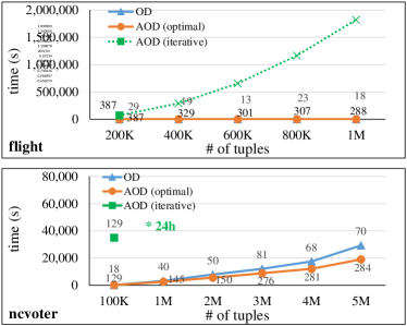
Figure 2. Scalability in $|\textbf{r}|$.

Exp-2: Scalability in $|{\mathchoice{\mbox{R}}{\mbox{R}}{\mbox{\scriptsize R}}{\mbox{\tiny R}}}|$. Next, we measure the runtime of the discovery framework in milliseconds, as illustrated in Figure 3. We use 1K tuples of our datasets (to allow experiments with a large number of attributes in reasonable time) and vary the number of attributes in multiples of five. In this experiment, the runtime has an exponential growth (the Y-axis in Figure 3 is in log scale). This is expected since the number of ODs increases exponentially with the number of tuples. The higher runtime on $\sf{ncvoter}$ compared to $\sf{flight}$ is attributed to having more ODs in higher levels of the lattice (with larger contexts).

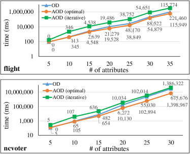
Figure 3. Scalability in $|\textbf{R}|$.

4.2. Comparison with the Iterative Algorithm

Exp-3: Runtime comparison with the iterative algorithm. As discussed in Section 3, our AOC validation algorithm has time complexity $\mathcal{O}(n\log n)$, while the iterative algorithm proposed in (Szlichta et al., 2017, 2018) has time complexity $\mathcal{O}(n\log n+\epsilon n^{2})$. Figures 2, 3, and 4 illustrate the running times of the AOD discovery framework when using these two validation algorithms.

As shown in Figure 2, while when using our algorithm, the framework can discover AOCs in datasets with up to millions of tuples, when using the iterative algorithm, it does not terminate within 24 hours on 400K and 1M tuples of the $\sf{flight}$ and $\sf{ncvoter}$ datasets, respectively (the running times for the $\sf{flight}$ dataset have been projected for better comparison). In cases where the framework equipped with the iterative algorithm terminates within the time limit, it is orders of magnitude slower. In Figure 3, while the differences are not as pronounced (as the number of tuples is too small), using our validation algorithm still makes the framework almost an order of magnitude faster.

We next experiment with the approximation threshold, by using 10K tuples from our datasets and setting the approximation threshold to 0, 5, 10, 15, 20, and 25 percent. As Figure 4 illustrates, while a larger approximation threshold does not increase the runtime of our algorithm (the runtime decreases in some cases due to better pruning opportunities), it increases the runtime of the iterative approach at an almost linear rate. This aligns with the time complexity of these algorithms, as analyzed in Section 3.

As mentioned in Section 1, validating AOCs becomes the bottleneck of the AOD discovery framework when using the iterative algorithm. This is verified in our experiments, as up to 99.6% of the total runtime is spent on validation. Using our LIS-based validation algorithm, we reduce the time spent on validating AOCs by up to 99.8%, which results in the orders-of-magnitude improvement in runtime discussed before.

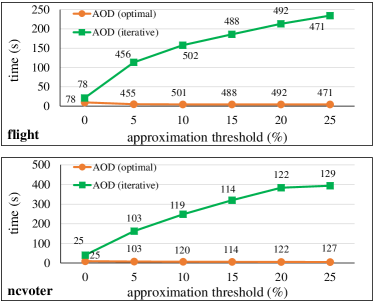
Figure 4. The effect of the approximation threshold.

Exp-4: Removal sets and validating AOCs using the iterative algorithm. While our validation algorithm guarantees finding a minimal removal set for a given OC (as is proved in Section 3.3), the iterative algorithm may overestimate the size of a minimal removal set. This results in removal sets which are on average around 1% larger than the true minimal removal set.

Overestimating the approximation factor may result in missing valid AOCs, if the true approximation factor is close to the input threshold. In Figures 2, 3, and 4, the numbers inside the plots indicate the number of OCs or AOCs found by an algorithm. We have not listed the number of approximate OFDs since this work focuses on discovering AOCs. (Wherever the plots for our algorithm and the algorithm for exact ODs overlap, the numbers on the bottom correspond to our approach.) In our experiments, the iterative approach misses up to 2% of the valid AOCs found using our optimal approach.

Missing these AOCs could have potentially severe consequences. For instance, in the $\sf{flight}$ dataset, the AOC of $\sf{arrivalDelay}\mathrel{\sim}\sf{lateAircraftDelay}$ holds with an approximation factor of 9.5%. This AOC points out that generally, delays in arrival are due to the aircraft and not other causes; e.g., security or weather delays. However, the iterative algorithm overestimates the approximation factor as 10.5%. This results in the framework missing this valid AOC when using an approximation threshold of 10%. Note that missing some AOCs results in different pruning opportunities, and, as a result, the set of discovered AOCs, which explains why the iterative algorithm discovers more AOCs in some cases.

Furthermore, as has been discussed for Exp-4.2, the running time of the iterative algorithm on larger datasets is prohibitively long. On such datasets, using the iterative algorithm results in missing all valid AOCs. For instance, in the $\sf{ncvoter}$ dataset with 5M tuples and with the approximation threshold set to 20%, the AOC of $\sf{municipalityAbbrv}\mathrel{\sim}\sf{municipalityDesc}$ is discovered, which points to exceptions in creating abbreviations for municipalities; e.g., “Raleigh” is abbreviated as “RAL”, while “Charlotte” is abbreviated as “CLT”. However, this AOC does not hold in our 100K sample of tuples when using this threshold. Therefore, this dependency would have been missed by using the iterative validation algorithm, as it exceeds the time limit on the full dataset.

4.3. Comparison with Exact OD Discovery

Exp-5: Lattice level of AOCs and runtime improvements. AOCs tend to reside in lower levels of the lattice (with smaller contexts). In our scalability experiments in the number of tuples (Exp-4.1), the AOCs are on average $1.2$ levels lower on the lattice. Similarly, in experiments in the number of attributes (Exp-2), the AOCs are on average $0.5$ levels lower on the lattice. Figure 5 shows the number of OCs or AOCs found at each level of the lattice, when using 5M tuples and 10 attributes of the $\sf{ncvoter}$ dataset. On this dataset, the average lattice level of the discovered dependencies drops from $5.6$ to $4.3$ when using our approximate algorithm. As discussed in (Szlichta et al., 2017) and (Szlichta et al., 2018), dependencies found in lower levels of the lattice are likely to be more interesting.

Furthermore, as discussed in Section 3.1, our discovery framework first validates candidates on lower levels of the lattice, and then applies pruning rules to generate the candidates on higher levels of the lattice. Therefore, by finding AOCs in lower levels, the algorithm can use pruning rules more effectively earlier in the discovery process, resulting in pruning some candidates on higher levels of the lattice. The effects of such pruning opportunities are not noticed when using the iterative validation algorithm, due to its prohibitively long running time. However, we optimally reduce the runtime of the validation step, resulting in runtime improvements for the discovery framework.

Figures 2 and 3 show the running times of the algorithms for discovering exact and approximate ODs. Even though validation of AOCs has a worse runtime compared to exact OCs, i.e., $\mathcal{O}(n\log n)$, as opposed to $\mathcal{O}(n)$, due to the extra pruning opportunities described above, the total runtime of the discovery framework for AODs can even be lower than the discovery framework for exact ODs; i.e., up to 34% and 76% faster in experiments in the number of tuples and attributes, respectively. The pronounced effect in the experiments in the number of attributes is due to having a smaller number of tuples.

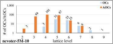
Figure 5. Number of discovered OCs/AOCs in each level.

Exp-6: Discovered AOCs compared to OCs. The exact algorithm fails to discover meaningful OCs in presence of anomalies, or even if a single value is erroneous. However, valid AOCs may hold in such instances. Other than the AOCs discussed in Exp-4, in the $\sf{flight}$ dataset, we discover the AOC $\sf{originAirport}\mathrel{\sim}\sf{IATACode}$ with an 8% approximation factor. This AOC can be used to identify data quality issues, as the airport identifier must uniquely correspond to the IATA code in ascending order. Furthermore, the AOC $\sf{streetAddress}\mathrel{\sim}\sf{mailAddress}$ holds in the $\sf{ncvoter}$ dataset with an approximation factor of 18%. This AOC can point to exceptions in address formats.

As shown in Figures 2 and 3, by discovering AOCs, we can find more dependencies in the data. Even if there are fewer AOCs than OCs (e.g., the $\sf{flight}$ dataset in Exp-2), the discovered dependencies are on lower levels of the lattice, as shown in Exp-4.3, which makes them more interesting (Szlichta et al., 2017, 2018). If the number of discovered dependencies is too large, the interestingness measure proposed in (Szlichta et al., 2018) can be used to rank the AOCs. In fact, the example AOCs that we have identified in Exp-4 and in this experiment, were all ranked as the most interesting AOCs based on this measure.

5. Conclusions

We proposed a new validation algorithm for approximate ODs and proved its minimality and runtime optimality. We then implemented our approach in an existing canonical OD discovery framework and demonstrated significant gains compared to existing frameworks for discovering exact and approximate OCs. In future work, we will study new approaches for discovering approximate OCs, such as hybrid sampling, as done in (Papenbrock and Naumann, 2016) for FDs. We will also extend our approximate OC discovery framework to distributed settings, similar to the work in (Saxena et al., 2019).

6. Appendix

Theorem 6.1.

The set s generated using Algorithm 2 is a minimal removal set with respect to the given AOC.

Proof
Since in the AOC validation problem the tuples within different partition groups with respect to the context are independent of each other. Without loss of generality, assume the OC candidate has an empty context and let $\sf{A}\mathrel{\sim}\sf{B}$ denote it. Let list $B$ denote the projection of tuples over $\sf{B}$ after ordering them by $\sf{A}$ and breaking ties by $\sf{B}$, and $L$ denote a LNDS of $B$. Let $L({\mathchoice{\mbox{\sf s}}{\mbox{\sf s}}{\mbox{\scriptsize\sf s}}{\mbox{\tiny\sf s}}})$ and $l_{i}$ denote the index of tuple s in $L$ (assuming s is in $L$) and the $i$-th element in $L$, respectively. Finally, let s be the minimal removal set found using our algorithm; i.e., the set of tuples not in $L$.

First, we prove that s is a removal set. Assume ${\mathchoice{\mbox{r}}{\mbox{r}}{\mbox{\scriptsize r}}{\mbox{\tiny r}}}\setminus{\mathchoice{\mbox{s}}{\mbox{s}}{\mbox{\scriptsize s}}{\mbox{\tiny s}}}\not\models\varphi$. Thus, there exist tuples ${\mathchoice{\mbox{\sf s}}{\mbox{\sf s}}{\mbox{\scriptsize\sf s}}{\mbox{\tiny\sf s}}},{\mathchoice{\mbox{\sf t}}{\mbox{\sf t}}{\mbox{\scriptsize\sf t}}{\mbox{\tiny\sf t}}}\in{\mathchoice{\mbox{r}}{\mbox{r}}{\mbox{\scriptsize r}}{\mbox{\tiny r}}}\setminus{\mathchoice{\mbox{s}}{\mbox{s}}{\mbox{\scriptsize s}}{\mbox{\tiny s}}}$ such that ${\mathchoice{\mbox{\sf{\sf s}}}{\mbox{\sf{\sf s}}}{\mbox{\scriptsize\sf{\sf s}}}{\mbox{\tiny\sf{\sf s}}}}_{\sf{A}}<{\mathchoice{\mbox{\sf{\sf t}}}{\mbox{\sf{\sf t}}}{\mbox{\scriptsize\sf{\sf t}}}{\mbox{\tiny\sf{\sf t}}}}_{\sf{A}}$ and ${\mathchoice{\mbox{\sf{\sf t}}}{\mbox{\sf{\sf t}}}{\mbox{\scriptsize\sf{\sf t}}}{\mbox{\tiny\sf{\sf t}}}}_{\sf{B}}<{\mathchoice{\mbox{\sf{\sf s}}}{\mbox{\sf{\sf s}}}{\mbox{\scriptsize\sf{\sf s}}}{\mbox{\tiny\sf{\sf s}}}}_{\sf{B}}$ (a swap). Since ${\mathchoice{\mbox{\sf s}}{\mbox{\sf s}}{\mbox{\scriptsize\sf s}}{\mbox{\tiny\sf s}}},{\mathchoice{\mbox{\sf t}}{\mbox{\sf t}}{\mbox{\scriptsize\sf t}}{\mbox{\tiny\sf t}}}\in{\mathchoice{\mbox{r}}{\mbox{r}}{\mbox{\scriptsize r}}{\mbox{\tiny r}}}\setminus{\mathchoice{\mbox{s}}{\mbox{s}}{\mbox{\scriptsize s}}{\mbox{\tiny s}}}$, ${\mathchoice{\mbox{\sf{\sf s}}}{\mbox{\sf{\sf s}}}{\mbox{\scriptsize\sf{\sf s}}}{\mbox{\tiny\sf{\sf s}}}}_{\sf{B}}$ and ${\mathchoice{\mbox{\sf{\sf t}}}{\mbox{\sf{\sf t}}}{\mbox{\scriptsize\sf{\sf t}}}{\mbox{\tiny\sf{\sf t}}}}_{\sf{B}}$ are in $L$. Moreover, because ${\mathchoice{\mbox{\sf{\sf s}}}{\mbox{\sf{\sf s}}}{\mbox{\scriptsize\sf{\sf s}}}{\mbox{\tiny\sf{\sf s}}}}_{\sf{A}}<{\mathchoice{\mbox{\sf{\sf t}}}{\mbox{\sf{\sf t}}}{\mbox{\scriptsize\sf{\sf t}}}{\mbox{\tiny\sf{\sf t}}}}_{\sf{A}}$, s is before t in the ordering and $L({\mathchoice{\mbox{\sf s}}{\mbox{\sf s}}{\mbox{\scriptsize\sf s}}{\mbox{\tiny\sf s}}})<L({\mathchoice{\mbox{\sf t}}{\mbox{\sf t}}{\mbox{\scriptsize\sf t}}{\mbox{\tiny\sf t}}})$. However, this means that $L$ is not nondecreasing, as ${\mathchoice{\mbox{\sf{\sf t}}}{\mbox{\sf{\sf t}}}{\mbox{\scriptsize\sf{\sf t}}}{\mbox{\tiny\sf{\sf t}}}}_{\sf{B}}<{\mathchoice{\mbox{\sf{\sf s}}}{\mbox{\sf{\sf s}}}{\mbox{\scriptsize\sf{\sf s}}}{\mbox{\tiny\sf{\sf s}}}}_{\sf{B}}$, which contradicts the assumption that $L$ is a LNDS of $B$. Therefore, ${\mathchoice{\mbox{r}}{\mbox{r}}{\mbox{\scriptsize r}}{\mbox{\tiny r}}}\setminus{\mathchoice{\mbox{s}}{\mbox{s}}{\mbox{\scriptsize s}}{\mbox{\tiny s}}}\models\varphi$.

Next, we prove that among all sets t such that ${\mathchoice{\mbox{r}}{\mbox{r}}{\mbox{\scriptsize r}}{\mbox{\tiny r}}}\setminus{\mathchoice{\mbox{t}}{\mbox{t}}{\mbox{\scriptsize t}}{\mbox{\tiny t}}}\models\varphi$, s has the smallest cardinality; i.e., it is a minimal removal set. Assume that a set ${\mathchoice{\mbox{s}}{\mbox{s}}{\mbox{\scriptsize s}}{\mbox{\tiny s}}}^{\prime}$ with $|{\mathchoice{\mbox{s}}{\mbox{s}}{\mbox{\scriptsize s}}{\mbox{\tiny s}}}^{\prime}|<|{\mathchoice{\mbox{s}}{\mbox{s}}{\mbox{\scriptsize s}}{\mbox{\tiny s}}}|$ exists, such that ${\mathchoice{\mbox{r}}{\mbox{r}}{\mbox{\scriptsize r}}{\mbox{\tiny r}}}\setminus{\mathchoice{\mbox{s}}{\mbox{s}}{\mbox{\scriptsize s}}{\mbox{\tiny s}}}^{\prime}\models\varphi$. Construct a subsequence $L^{\prime}$ of $B$ by including the projection of tuples that do not exist in ${\mathchoice{\mbox{s}}{\mbox{s}}{\mbox{\scriptsize s}}{\mbox{\tiny s}}}^{\prime}$. Because $|{\mathchoice{\mbox{s}}{\mbox{s}}{\mbox{\scriptsize s}}{\mbox{\tiny s}}}^{\prime}|<|{\mathchoice{\mbox{s}}{\mbox{s}}{\mbox{\scriptsize s}}{\mbox{\tiny s}}}|$, $L^{\prime}$ is longer than $L$. Since ${\mathchoice{\mbox{r}}{\mbox{r}}{\mbox{\scriptsize r}}{\mbox{\tiny r}}}\setminus{\mathchoice{\mbox{s}}{\mbox{s}}{\mbox{\scriptsize s}}{\mbox{\tiny s}}}^{\prime}\models\varphi$, there do not exist tuples ${\mathchoice{\mbox{\sf s}}{\mbox{\sf s}}{\mbox{\scriptsize\sf s}}{\mbox{\tiny\sf s}}},{\mathchoice{\mbox{\sf t}}{\mbox{\sf t}}{\mbox{\scriptsize\sf t}}{\mbox{\tiny\sf t}}}\in{\mathchoice{\mbox{r}}{\mbox{r}}{\mbox{\scriptsize r}}{\mbox{\tiny r}}}\setminus{\mathchoice{\mbox{s}}{\mbox{s}}{\mbox{\scriptsize s}}{\mbox{\tiny s}}}^{\prime}$ such that ${\mathchoice{\mbox{\sf{\sf s}}}{\mbox{\sf{\sf s}}}{\mbox{\scriptsize\sf{\sf s}}}{\mbox{\tiny\sf{\sf s}}}}_{\sf{A}}<{\mathchoice{\mbox{\sf{\sf t}}}{\mbox{\sf{\sf t}}}{\mbox{\scriptsize\sf{\sf t}}}{\mbox{\tiny\sf{\sf t}}}}_{\sf{A}}$ and ${\mathchoice{\mbox{\sf{\sf t}}}{\mbox{\sf{\sf t}}}{\mbox{\scriptsize\sf{\sf t}}}{\mbox{\tiny\sf{\sf t}}}}_{\sf{B}}<{\mathchoice{\mbox{\sf{\sf s}}}{\mbox{\sf{\sf s}}}{\mbox{\scriptsize\sf{\sf s}}}{\mbox{\tiny\sf{\sf s}}}}_{\sf{B}}$. Furthermore, since the tuples are order by $\sf{A}$ and ties are broken by $\sf{B}$, $L({\mathchoice{\mbox{\sf s}}{\mbox{\sf s}}{\mbox{\scriptsize\sf s}}{\mbox{\tiny\sf s}}})<L({\mathchoice{\mbox{\sf t}}{\mbox{\sf t}}{\mbox{\scriptsize\sf t}}{\mbox{\tiny\sf t}}})$ for all ${\mathchoice{\mbox{\sf s}}{\mbox{\sf s}}{\mbox{\scriptsize\sf s}}{\mbox{\tiny\sf s}}},{\mathchoice{\mbox{\sf t}}{\mbox{\sf t}}{\mbox{\scriptsize\sf t}}{\mbox{\tiny\sf t}}}\in{\mathchoice{\mbox{r}}{\mbox{r}}{\mbox{\scriptsize r}}{\mbox{\tiny r}}}\setminus{\mathchoice{\mbox{s}}{\mbox{s}}{\mbox{\scriptsize s}}{\mbox{\tiny s}}}^{\prime}$ such that ${\mathchoice{\mbox{\sf{\sf s}}}{\mbox{\sf{\sf s}}}{\mbox{\scriptsize\sf{\sf s}}}{\mbox{\tiny\sf{\sf s}}}}_{\sf{A}}={\mathchoice{\mbox{\sf{\sf t}}}{\mbox{\sf{\sf t}}}{\mbox{\scriptsize\sf{\sf t}}}{\mbox{\tiny\sf{\sf t}}}}_{\sf{A}}$ and ${\mathchoice{\mbox{\sf{\sf s}}}{\mbox{\sf{\sf s}}}{\mbox{\scriptsize\sf{\sf s}}}{\mbox{\tiny\sf{\sf s}}}}_{\sf{B}}<{\mathchoice{\mbox{\sf{\sf t}}}{\mbox{\sf{\sf t}}}{\mbox{\scriptsize\sf{\sf t}}}{\mbox{\tiny\sf{\sf t}}}}_{\sf{B}}$. Therefore, there do not exist $i<j$ such that $l^{\prime}_{j}<l^{\prime}_{i}$. Thus, $L^{\prime}$ is a nondecreasing subsequence of $B$ which is longer than $L$. This is in contradiction with $L$ being a LNDS of $B$. Therefore, s has the smallest size possible for a removal set. $\Box$

Theorem 6.2.

Algorithm 2 has the optimal runtime for validating an AOC candidate.

Proof
In (Fredman, 1975), the author has proved an $\Omega(n\log n)$ lower bound for a decision variant of the LIS problem, here referred to as LIS-DEC, as follows: given a list of $n$ distinct values, is the length of a longest increasing subsequence, denoted by $|L|$, larger than or equal to $k=\lfloor 3n^{1/2}\rfloor$? To prove the same lower bound for the AOC validation problem (and thus, the optimality of our algorithm), we offer a linear-time mapping from instances of LIS-DEC to AOC validation instances, in which $|L|\geq k$ iff the AOC instance is valid with an approximation threshold of $1-k/n$.

Let $B$ be the input list for a LIS-DEC instance, consisting of $[b_{1},$ $b_{2},$ $\dots,$ $b_{n}]$. For the corresponding AOC instance, let r be a table with attributes $\sf{A}$ and $\sf{B}$, and consider the OC $\sf{A}\mathrel{\sim}\sf{B}$, denoted by $\varphi$. For each $b_{i}\in B$, add the tuple ${\mathchoice{\mbox{\sf t}}{\mbox{\sf t}}{\mbox{\scriptsize\sf t}}{\mbox{\tiny\sf t}}}_{i}$ $=$ $(i,b_{i})$ to r.

We first prove that if the AOC candidate is valid, then the LIS-DEC instance holds; i.e., if $e(\varphi)\leq 1-k/n$, then $|L|\geq k$. Let s be a minimal removal set with respect to $\sf{A}\mathrel{\sim}\sf{B}$. Since the AOC candidate is valid, $|{\mathchoice{\mbox{s}}{\mbox{s}}{\mbox{\scriptsize s}}{\mbox{\tiny s}}}|\leq n-k$. We now create $L$, a subsequence of $B$, which contains all $b_{i}$’s where ${\mathchoice{\mbox{\sf t}}{\mbox{\sf t}}{\mbox{\scriptsize\sf t}}{\mbox{\tiny\sf t}}}_{i}\not\in{\mathchoice{\mbox{s}}{\mbox{s}}{\mbox{\scriptsize s}}{\mbox{\tiny s}}}$. Since $|L|=n-|{\mathchoice{\mbox{s}}{\mbox{s}}{\mbox{\scriptsize s}}{\mbox{\tiny s}}}|$, we know that $|L|\geq k$. Therefore, we only need to prove that $L$ is an increasing subsequence of $B$. Assume $L$ is not increasing; therefore, there exist $b_{i},b_{j}\in L$ such that $i<j$ and $b_{j}<b_{i}$. Since $b_{i},b_{j}\in L$, ${\mathchoice{\mbox{\sf t}}{\mbox{\sf t}}{\mbox{\scriptsize\sf t}}{\mbox{\tiny\sf t}}}_{i},{\mathchoice{\mbox{\sf t}}{\mbox{\sf t}}{\mbox{\scriptsize\sf t}}{\mbox{\tiny\sf t}}}_{j}\in{\mathchoice{\mbox{r}}{\mbox{r}}{\mbox{\scriptsize r}}{\mbox{\tiny r}}}\setminus{\mathchoice{\mbox{s}}{\mbox{s}}{\mbox{\scriptsize s}}{\mbox{\tiny s}}}$. However, ${\mathchoice{\mbox{\sf${\mathchoice{\mbox{\sf t}}{\mbox{\sf t}}{\mbox{\scriptsize\sf t}}{\mbox{\tiny\sf t}}}_{i}$}}{\mbox{\sf${\mathchoice{\mbox{\sf t}}{\mbox{\sf t}}{\mbox{\scriptsize\sf t}}{\mbox{\tiny\sf t}}}_{i}$}}{\mbox{\scriptsize\sf${\mathchoice{\mbox{\sf t}}{\mbox{\sf t}}{\mbox{\scriptsize\sf t}}{\mbox{\tiny\sf t}}}_{i}$}}{\mbox{\tiny\sf${\mathchoice{\mbox{\sf t}}{\mbox{\sf t}}{\mbox{\scriptsize\sf t}}{\mbox{\tiny\sf t}}}_{i}$}}}_{\sf{A}}<{\mathchoice{\mbox{\sf${\mathchoice{\mbox{\sf t}}{\mbox{\sf t}}{\mbox{\scriptsize\sf t}}{\mbox{\tiny\sf t}}}_{j}$}}{\mbox{\sf${\mathchoice{\mbox{\sf t}}{\mbox{\sf t}}{\mbox{\scriptsize\sf t}}{\mbox{\tiny\sf t}}}_{j}$}}{\mbox{\scriptsize\sf${\mathchoice{\mbox{\sf t}}{\mbox{\sf t}}{\mbox{\scriptsize\sf t}}{\mbox{\tiny\sf t}}}_{j}$}}{\mbox{\tiny\sf${\mathchoice{\mbox{\sf t}}{\mbox{\sf t}}{\mbox{\scriptsize\sf t}}{\mbox{\tiny\sf t}}}_{j}$}}}_{\sf{A}}$, while ${\mathchoice{\mbox{\sf${\mathchoice{\mbox{\sf t}}{\mbox{\sf t}}{\mbox{\scriptsize\sf t}}{\mbox{\tiny\sf t}}}_{j}$}}{\mbox{\sf${\mathchoice{\mbox{\sf t}}{\mbox{\sf t}}{\mbox{\scriptsize\sf t}}{\mbox{\tiny\sf t}}}_{j}$}}{\mbox{\scriptsize\sf${\mathchoice{\mbox{\sf t}}{\mbox{\sf t}}{\mbox{\scriptsize\sf t}}{\mbox{\tiny\sf t}}}_{j}$}}{\mbox{\tiny\sf${\mathchoice{\mbox{\sf t}}{\mbox{\sf t}}{\mbox{\scriptsize\sf t}}{\mbox{\tiny\sf t}}}_{j}$}}}_{\sf{B}}<{\mathchoice{\mbox{\sf${\mathchoice{\mbox{\sf t}}{\mbox{\sf t}}{\mbox{\scriptsize\sf t}}{\mbox{\tiny\sf t}}}_{i}$}}{\mbox{\sf${\mathchoice{\mbox{\sf t}}{\mbox{\sf t}}{\mbox{\scriptsize\sf t}}{\mbox{\tiny\sf t}}}_{i}$}}{\mbox{\scriptsize\sf${\mathchoice{\mbox{\sf t}}{\mbox{\sf t}}{\mbox{\scriptsize\sf t}}{\mbox{\tiny\sf t}}}_{i}$}}{\mbox{\tiny\sf${\mathchoice{\mbox{\sf t}}{\mbox{\sf t}}{\mbox{\scriptsize\sf t}}{\mbox{\tiny\sf t}}}_{i}$}}}_{\sf{B}}$. Thus, there exists a swap with respect to $\sf{A}\mathrel{\sim}\sf{B}$ in ${\mathchoice{\mbox{r}}{\mbox{r}}{\mbox{\scriptsize r}}{\mbox{\tiny r}}}\setminus{\mathchoice{\mbox{s}}{\mbox{s}}{\mbox{\scriptsize s}}{\mbox{\tiny s}}}$, which contradicts the assumption that s is a removal set w.r.t.  $\sf{A}\mathrel{\sim}\sf{B}$. Therefore, $L$ is an increasing subsequence of $B$ and the LIS-DEC instance holds.

We now prove the other direction, i.e., if the LIS-DEC holds, then the AOC candidate is valid. Let $L$ be a longest increasing subsequence of $B$, where $|L|\geq k$. We construct a set of tuples s, by including all tuples ${\mathchoice{\mbox{\sf t}}{\mbox{\sf t}}{\mbox{\scriptsize\sf t}}{\mbox{\tiny\sf t}}}_{i}\in{\mathchoice{\mbox{r}}{\mbox{r}}{\mbox{\scriptsize r}}{\mbox{\tiny r}}}$, where $b_{i}\not\in L$. We know that $|{\mathchoice{\mbox{s}}{\mbox{s}}{\mbox{\scriptsize s}}{\mbox{\tiny s}}}|/n\leq 1-k/n$ since $|{\mathchoice{\mbox{s}}{\mbox{s}}{\mbox{\scriptsize s}}{\mbox{\tiny s}}}|=n-|L|$. Therefore, to prove that the AOC candidate is valid, we only need show that s is a removal set with respect to t and $\varphi$; i.e., ${\mathchoice{\mbox{r}}{\mbox{r}}{\mbox{\scriptsize r}}{\mbox{\tiny r}}}\setminus{\mathchoice{\mbox{s}}{\mbox{s}}{\mbox{\scriptsize s}}{\mbox{\tiny s}}}\models\varphi$. Assume s is not a removal set. Thus, there exist tuples ${\mathchoice{\mbox{\sf t}}{\mbox{\sf t}}{\mbox{\scriptsize\sf t}}{\mbox{\tiny\sf t}}}_{i},{\mathchoice{\mbox{\sf t}}{\mbox{\sf t}}{\mbox{\scriptsize\sf t}}{\mbox{\tiny\sf t}}}_{j}\in{\mathchoice{\mbox{r}}{\mbox{r}}{\mbox{\scriptsize r}}{\mbox{\tiny r}}}\setminus{\mathchoice{\mbox{s}}{\mbox{s}}{\mbox{\scriptsize s}}{\mbox{\tiny s}}}$ such that $i<j$ (and therefore, ${\mathchoice{\mbox{\sf${\mathchoice{\mbox{\sf t}}{\mbox{\sf t}}{\mbox{\scriptsize\sf t}}{\mbox{\tiny\sf t}}}_{i}$}}{\mbox{\sf${\mathchoice{\mbox{\sf t}}{\mbox{\sf t}}{\mbox{\scriptsize\sf t}}{\mbox{\tiny\sf t}}}_{i}$}}{\mbox{\scriptsize\sf${\mathchoice{\mbox{\sf t}}{\mbox{\sf t}}{\mbox{\scriptsize\sf t}}{\mbox{\tiny\sf t}}}_{i}$}}{\mbox{\tiny\sf${\mathchoice{\mbox{\sf t}}{\mbox{\sf t}}{\mbox{\scriptsize\sf t}}{\mbox{\tiny\sf t}}}_{i}$}}}_{\sf{A}}<{\mathchoice{\mbox{\sf${\mathchoice{\mbox{\sf t}}{\mbox{\sf t}}{\mbox{\scriptsize\sf t}}{\mbox{\tiny\sf t}}}_{j}$}}{\mbox{\sf${\mathchoice{\mbox{\sf t}}{\mbox{\sf t}}{\mbox{\scriptsize\sf t}}{\mbox{\tiny\sf t}}}_{j}$}}{\mbox{\scriptsize\sf${\mathchoice{\mbox{\sf t}}{\mbox{\sf t}}{\mbox{\scriptsize\sf t}}{\mbox{\tiny\sf t}}}_{j}$}}{\mbox{\tiny\sf${\mathchoice{\mbox{\sf t}}{\mbox{\sf t}}{\mbox{\scriptsize\sf t}}{\mbox{\tiny\sf t}}}_{j}$}}}_{\sf{A}}$), but ${\mathchoice{\mbox{\sf${\mathchoice{\mbox{\sf t}}{\mbox{\sf t}}{\mbox{\scriptsize\sf t}}{\mbox{\tiny\sf t}}}_{j}$}}{\mbox{\sf${\mathchoice{\mbox{\sf t}}{\mbox{\sf t}}{\mbox{\scriptsize\sf t}}{\mbox{\tiny\sf t}}}_{j}$}}{\mbox{\scriptsize\sf${\mathchoice{\mbox{\sf t}}{\mbox{\sf t}}{\mbox{\scriptsize\sf t}}{\mbox{\tiny\sf t}}}_{j}$}}{\mbox{\tiny\sf${\mathchoice{\mbox{\sf t}}{\mbox{\sf t}}{\mbox{\scriptsize\sf t}}{\mbox{\tiny\sf t}}}_{j}$}}}_{\sf{B}}<{\mathchoice{\mbox{\sf${\mathchoice{\mbox{\sf t}}{\mbox{\sf t}}{\mbox{\scriptsize\sf t}}{\mbox{\tiny\sf t}}}_{i}$}}{\mbox{\sf${\mathchoice{\mbox{\sf t}}{\mbox{\sf t}}{\mbox{\scriptsize\sf t}}{\mbox{\tiny\sf t}}}_{i}$}}{\mbox{\scriptsize\sf${\mathchoice{\mbox{\sf t}}{\mbox{\sf t}}{\mbox{\scriptsize\sf t}}{\mbox{\tiny\sf t}}}_{i}$}}{\mbox{\tiny\sf${\mathchoice{\mbox{\sf t}}{\mbox{\sf t}}{\mbox{\scriptsize\sf t}}{\mbox{\tiny\sf t}}}_{i}$}}}_{\sf{B}}$. Since ${\mathchoice{\mbox{\sf t}}{\mbox{\sf t}}{\mbox{\scriptsize\sf t}}{\mbox{\tiny\sf t}}}_{i},{\mathchoice{\mbox{\sf t}}{\mbox{\sf t}}{\mbox{\scriptsize\sf t}}{\mbox{\tiny\sf t}}}_{j}\in{\mathchoice{\mbox{r}}{\mbox{r}}{\mbox{\scriptsize r}}{\mbox{\tiny r}}}\setminus{\mathchoice{\mbox{s}}{\mbox{s}}{\mbox{\scriptsize s}}{\mbox{\tiny s}}}$, $b_{i}$ and $b_{j}$ are in $L$. Therefore, there exist values $b_{i}$ and $b_{j}$ in $L$ such that $i<j$, but $b_{j}<b_{i}$. Thus, $L$ is not increasing, which is in contradiction with the assumption that $L$ is a LIS of $B$. Therefore, ${\mathchoice{\mbox{r}}{\mbox{r}}{\mbox{\scriptsize r}}{\mbox{\tiny r}}}\setminus{\mathchoice{\mbox{s}}{\mbox{s}}{\mbox{\scriptsize s}}{\mbox{\tiny s}}}\models\varphi$ and the AOC candidate is valid.

Therefore, the LIS-DEC instance holds if and only if the corresponding AOC candidate is valid. Since the mapping takes linear time in the size of the input, $\Omega(n\log n)$ is also a lower bound for the AOC validation problem. $\Box$

References

- (1)
- Consonni et al. (2019) C. Consonni, P. Sottovia, A. Montresor, and Y. Velegrakis. 2019. Discovering order dependencies through order compatibility. In EDBT. 409–420.
- Fredman (1975) M. Fredman. 1975. On computing the length of longest increasing subsequences. Discrete Mathematics 11, 1 (1975), 29 – 35.
- Huhtala et al. (1999) Y. Huhtala, J. Kärkkäinen, P. Porkka, and H. Toivonen. 1999. TANE: An Efficient Algorithm for Discovering Functional and Approximate Dependencies. Comput. J. 42 (1999), 100–111.
- Jin et al. (2020) Yifeng Jin, L. Zhu, and Zijing Tan. 2020. Efficient Bidirectional Order Dependency Discovery. 2020 IEEE 36th International Conference on Data Engineering (ICDE) (2020), 61–72.
- Langer and Naumann (2016) P. Langer and F. Naumann. 2016. Efficient Order Dependency Detection. The VLDB Journal 25, 2 (April 2016), 223–241.
- Papenbrock and Naumann (2016) T. Papenbrock and F. Naumann. 2016. A Hybrid Approach to Functional Dependency Discovery. In Proceedings of the 2016 International Conference on Management of Data (SIGMOD ’16). Association for Computing Machinery, New York, NY, USA, 821–833.
- Qiu et al. (2018) Y. Qiu, Tan, K. Z., Yang, X. Yang, and N. Guo. 2018. Repairing data violations with order dependencies. In DASFAA. 283–300.
- Saxena et al. (2019) H. Saxena, L. Golab, and I. Ilyas. 2019. Distributed Implementations of Dependency Discovery Algorithms. Proc. VLDB Endow. 12, 11 (July 2019), 1624–1636.
- Szlichta et al. (2017) J. Szlichta, P. Godfrey, L. Golab, M. Kargar, and D. Srivastava. 2017. Effective and complete discovery of order dependencies via set-based axiomatization. PVLDB 10, 7 (2017), 721–732.
- Szlichta et al. (2018) J. Szlichta, P. Godfrey, L. Golab, M. Kargar, and D. Srivastava. 2018. Effective and Complete Discovery of Bidirectional Order Dependencies via Set-Based Axioms. The VLDB Journal 27, 4 (Aug. 2018), 573–591.
- Szlichta et al. (2020) J. Szlichta, P. Godfrey, L. Golab, M. Kargar, and D. Srivastava. 2020. Erratum for discovering order dependencies through order compatibility. In EDBT. 659–663.
- Szlichta et al. (2012) J. Szlichta, P. Godfrey, and J. Gryz. 2012. Fundamentals of Order Dependencies. Proc. VLDB Endow. 5, 11 (July 2012), 1220–1231.