Scalable Feature Matching Across Large Data Collections

Abstract

This paper is concerned with matching feature vectors in a one-to-one fashion across large collections of datasets. Formulating this task as a multidimensional assignment problem with decomposable costs (MDADC), we develop extremely fast algorithms with time complexity linear in the number $n$ of datasets and space complexity a small fraction of the data size. These remarkable properties hinge on using the squared Euclidean distance as dissimilarity function, which can reduce ${n\choose 2}$ matching problems between pairs of datasets to $n$ problems and enable calculating assignment costs on the fly. To our knowledge, no other method applicable to the MDADC possesses these linear scaling and low-storage properties necessary to large-scale applications. In numerical experiments, the novel algorithms outperform competing methods and show excellent computational and optimization performances. An application of feature matching to a large neuroimaging database is presented. The algorithms of this paper are implemented in the R package matchFeat available at github.com/ddegras/matchFeat.

1 Introduction

Matching objects across units (e.g. subjects, digital images, or networks) based on common descriptor variables is an ubiquitous task in applied science. This problem, variously known as object matching, feature matching, data association, or assignment problem, is at the core of applications such as resource allocation (Pierskalla, 1968), object tracking (Thornbrue et al., 2010; Bar-Shalom et al., 2011; Dehghan et al., 2015; Rezatofighi et al., 2015; Smeulders et al., 2014; Wang et al., 2015), object recognition (Lowe, 2001; Belongie et al., 2002; Conte et al., 2004), navigation systems (Doherty et al., 2019), image registration (Le Moigne et al., 2011; Ashburner, 2007), optimization of communication networks (Shalom et al., 2010), connectomics in neuroscience (Haxby et al., 2011; Vogelstein et al., 2015), and more.

The impetus for this work is a task in functional neuroimaging which consists in matching collections of biomarkers (more precisely, brain connectivity measures) between the subjects of a study. The matching process may serve in data exploration to provide new scientific insights and generate hypotheses. It can also be a preliminary step in a group analysis to ensure meaningful comparisons across subjects. Key aspects of the matching problem under study are that: (i) the number of subjects and/or the number of biomarkers per subject may be large, posing computational challenges, (ii) for two given subjects, each biomarker of one subject must be matched to at most one biomarker of the other (one-to-one matching), and (iii) the matching must be consistent, i.e. transitive across subjects (for example, denoting subjects by letters and biomarkers by numbers, if A1 is matched to B2 and B2 to C3, then A1 must be matched to C3). This matching problem is not specific to neuroimaging and is applicable to the research fields mentioned above. It is generally relevant to multilevel or hierarchical analyses where outputs of a certain level of analysis must be matched before becoming inputs at the next level. This situation typically occurs when the outputs to be matched result from an unsupervised analysis such as clustering, segmentation, or dimension reduction.

Problem formulation.

The matching problem at the core of this paper is as follows. Given $n$ set of vectors in $\mathbb{R}^{p}$ having the same size, say $\{x_{11},\ldots,x_{1m}\},\ldots,\{x_{n1},\ldots,x_{nm}\}$, find permutations $\sigma_{1},\ldots,\sigma_{n}$ of the vector labels $\{1,\ldots,m\}$ that minimize the sum of pairwise squared Euclidean distances within clusters $\{x_{1\sigma_{1}(k)},\ldots,x_{n\sigma_{n}(k)}\}$ ($1\leq k\leq m$). Writing $[r]=\{1,\ldots,r\}$ for a positive integer $r$ and letting $\mathbf{S}_{m}$ be the set of all permutations of $[m]$, the problem expresses as

$$\min_{\sigma_{1},\ldots,\sigma_{n}\in\mathbf{S}_{m}}\sum_{1\leq i<j\leq n}\sum_{k=1}^{m}\big{\|}x_{i\sigma_{i}(k)}-x_{j\sigma_{j}(k)}\big{\|}^{2}$$ (1)

where $\|\cdot\|$ denotes the Euclidean norm on $\mathbb{R}^{p}$.

Problem (1) is a sum-of-squares clustering problem with the constraint that each cluster must contain exactly one vector from each set $\{x_{i1},\ldots,x_{im}\}$, $i\in[n]$. Identifying the $n$ sets with statistical units, this constraint guarantees that the obtained clusters reflect common patterns between units, not within units. For this reason, one-to-one feature matching is particularly suitable in applications where variations between units dominate variations within units.

In problem (1), all statistical units have the same number $m$ of vectors. It is natural to also set to $m$ the number of clusters to partition the vectors into. In practice however, statistical units may have unbalanced numbers of observations, say $m_{1},\ldots,m_{n}$. It may also be desirable to group the observations in an arbitrary number of clusters, say $K$. Accordingly, a more general version of problem (1) would be, for each $i\in[n]$, to assign vectors $x_{i1},\ldots,x_{im_{i}}$ to $K$ clusters in a one-to-one fashion so as to minimize the total sum of pairwise squared Euclidean distances within clusters. Here, one-to-one means that each unit $i$ can contribute at most one vector to any cluster: if $m_{i}=K$, each vector from unit $i$ is assigned to a cluster and each cluster contains exactly one vector from unit $i$; if $m_{i}<K$, some clusters do not contain vectors from unit $i$; and if $m_{i}>K$, some vectors from unit $i$ are not assigned to a cluster, i.e. they are unmatched. The matching problem (1) thus generalizes as

$$\min_{s_{1},\ldots,s_{n}}\sum_{1\leq i<j\leq n}\sum_{k=1}^{K}\sum_{\begin{subarray}{c}q\in[m_{i}],r\in[m_{j}]\\ s_{i}(q)=s_{j}(r)=k\end{subarray}}\left\|x_{iq}-x_{jr}\right\|^{2}$$ (2)

where each $s_{i}$ is a map from the set $[m_{i}]$ of vector labels to the set $\{0,\ldots,K\}$ of cluster labels where, by convention, labels of unassigned/unmatched vectors are mapped to the cluster label 0. The map $s_{i}$ is such that $s_{i}(q)=s_{i}(r)$ implies that $q=r$ or $s_{i}(q)=s_{i}(r)=0$. In other words the restriction of $s_{i}$ to $[m_{i}]\setminus s_{i}^{-1}(\{0\})$ must be an injective map. Problem (1) is recovered when $m_{1}=\cdots=m_{n}=K:=m$, in which case $s_{i}=\sigma_{i}^{-1}$ for all $i\in[n]$.

For simplicity, only problem (1) is treated in this paper. However, the proposed matching methods extend to the general problem (2). In complement to the model-free problem (1), a probabilistic approach to feature matching based on Gaussian mixtures is detailed in Section 2.5.

Related work.

Problem (1) can be viewed through the prism of combinatorial optimization problems such as the minimum weight clique partitioning problem in a complete $n$-partite graph, the quadratic assignment problem (Koopmans and Beckmann, 1957; Çela, 1998), or the multidimensional assignment problem (MAP) (e.g. Burkard et al., 2009). The MAP formalism is well suited to this work and is recalled hereafter:

$$\min_{\sigma_{1},\ldots,\sigma_{n}\in\mathbf{S}_{m}}\sum_{k=1}^{m}c_{\sigma_{1}(k)\sigma_{2}(k)\cdots\sigma_{n}(k)}$$ (3)

where $(c_{a_{1}a_{2}\ldots a_{n}})\in\mathbb{R}^{m^{n}}$ is an $n$-dimensional array containing the costs of assigning the feature vectors $x_{1a_{1}},\ldots,x_{na_{n}}$ to the same cluster. Problem (1) is an instance of the MAP and, more precisely, it is a multidimensional assignment problem with decomposable costs (MDADC) (e.g. Bandelt et al., 1994, 2004) because its assignment costs decompose as

$$c_{a_{1}a_{2}\ldots i_{n}}=\sum_{1\leq i<j\leq n}d(x_{ia_{i}},x_{ja_{j}})$$ (4)

where $d$ is a dissimilarity function. The squared Euclidean distance $d$ used in (1) enables the development of highly efficient computational methods (see Section 2). The need for efficient computations comes from the exponential size $(m!)^{n}$ of the search domain $(\mathbf{S}_{m})^{n}$ and from the NP-hardness of (1) (when $n\geq 3$) as a generalization of the 3D assignment problem of Spieksma and Woeginger (1996).

The formidable literature on the MAP, which spans more than five decades and multiple mathematical fields, will not be reviewed here. The interested reader may fruitfully consult Burkard et al. (2009) and Pardalos and Pitsoulis (2000). In fact, given the focus of the present work on computations, a broad review of the general MAP is not necessary. Indeed, optimization methods for the MAP (e.g. Karapetyan and Gutin, 2011; Pierskalla, 1968; Poore and Rijavec, 1993; Robertson, 2001) are not computationally efficient for the special case of MDADC (and in particular (1)), especially if the number $n$ of dimensions is large. We will therefore only discuss the relevant MDADC literature.

Bandelt et al. (1994) provide simple “hub” and “recursive” heuristics for the MDADC (3)-(4) along with their approximation ratios (worst-case bounds on the ratio of a method’s attained objective to the optimal objective value). The hub heuristic consists in selecting one dimension $i\in[n]$ of the MDADC as a “hub” and matching all other dimensions to this one, i.e. finding for each dimension $j\neq i$ the assignment that minimizes the total cost with respect to $i$. The recursive heuristic starts by permuting the $n$ dimensions of the problem and then recursively finds the best assignment for the $i$th permuted dimension with respect to the $(i-1)$ first permuted dimensions ($i=2,\ldots,n$). Bandelt et al. (2004) enhance the heuristic methods of Bandelt et al. (1994) with local neighborhood search methods that attempt to improve a solution one or two dimensions at a time. They derive lower bounds for the minimum cost assignment based on a Lagrangian relaxation of the MDADC. Collins (2012) also exploits the idea of improving solutions one dimension at a time in the general MAP (3) through a factorization technique. Kuroki and Matsui (2009) formulate (1) as the problem of finding a clique cover of an $n$-partite graph with minimum edge weights. They express the clique cover problem with various mathematical programs (integer linear, nonconvex quadratic, integer quadratic, and second order cone) which they tackle directly or after relaxation. They also provide approximation ratios and computational complexity bounds for their algorithms. Tauer and Nagi (2013) and Natu et al. (2020) solve Lagrangian relaxations of the integer linear program formulation of the MDADC, with an emphasis on efficient parallel computation in a Map-Reduce framework or with GPUs. They derive tight lower bounds to control the approximation error of their algorithms.

As an alternative from the multidimensional assignment perspective, problem (1) can be viewed as an instance of constrained clustering or semi-supervised learning (Basu et al., 2009; Gancarski et al., 2020). The constraint that each unit $i\in[n]$ contributes exactly one feature vector to each cluster can be rephrased as: two vector instances from the same unit cannot be assigned to the same cluster. This type of constraint, namely that certain pairs of instances cannot be assigned to the same cluster (“cannot link” constraint) or that certain pairs must be assigned to the same cluster (“must link” constraint), is called equivalence constraints and can be handled by constrained $K$-means algorithms (Wagstaff et al., 2001; Bilenko et al., 2004; Pelleg and Baras, 2007) or through constrained mixture models (Shental et al., 2004).

Other tasks related to problem (1) but not directly relevant are object tracking, with applications in engineering and more recently in computer vision and artificial intelligence, and image registration, which plays a key role in image processing, object recognition, and remote sensing. The former involves a temporal dimension absent from (1) whereas the latter involves many (and often noisy) features that are not matched one-to-one. Matching problems also have a long history in statistics and have been a topic of intense scrutiny in machine learning in recent years (DeGroot and Goel, 1976; Collier and Dalalyan, 2016; Hsu et al., 2017; Pananjady et al., 2018). However, much of the research in these fields relevant to (1) deals with the case where $n=2$ and $m$ is large (asymptotically $m\to\infty$) whereas we are chiefly interested in situations where $m$ is fixed and $n$ is large ($n\to\infty$).

Contributions.

The methods for the MDADC (3)-(4) discussed heretofore are applied in practice to problems of small size, say $n$ in the single digits or a few tens. Theoretical considerations as well as numerical experiments from this paper (see Sections 2-3) and from the literature indicate that these methods cannot handle large-scale problems with $n$ in the hundreds, thousands or more (at least, not in a reasonable time on a single computer). As a simple example, the ${n\choose 2}m^{2}$ costs in (4) are typically calculated and stored before starting the optimization, but even this preliminary step may exceed computer memory limits for large $n$ and/or $m$. In response to this methodological gap, our research aims to develop fast, scalable methods for matching feature vectors in a one-to-one fashion across a large number of statistical units. The main contributions of the paper are the following.

1. We develop very fast algorithms for solving the matching problem (1), that is, (3)-(4) with $d$ as the squared Euclidean distance. The three main algorithms (Sections 2.1-2.2-2.3) have iteration complexity $O(nm^{3})$ and only take a few iterations to converge, meaning that they scale linearly with $n$. In addition, they calculate assignment costs (4) on the fly and have space requirements $O(mn+mp)$, a fraction of the data size $mnp$. We also present initialization methods and a refinement method (pairwise interchange). Further, we take a probabilistic view of (1) as a constrained Gaussian mixture model and devise an efficient implementation of the Expectation-Maximization (EM) algorithm.

2. We provide a broad review of the diverse methods applicable to (1) (integer linear programming, various relaxations, constrained clustering) which rarely appear together in a paper. The novel algorithms are compared to these methods in numerical experiments and show excellent computation and optimization performances.

3. An R package matchFeat implementing all the algorithms of the paper is made available at github.com/ddegras/matchFeat.

4. The matching problem (1) is applied to a large database of neuroimaging data to study functional connectivity in the human brain. The data analysis confirms existing knowledge but also generates new insights, thus demonstrating the practical usefulness of our approach.

Organization of the paper.

Section 2 introduces novel algorithms for the matching problem (1). In Section 3, a numerical study assesses the novel algorithms and competing methods with respect to computation and optimization performance. Section 4 details an application of our matching approach to a large neuroimaging database (ABIDE) relating to autism spectrum disorders. Concluding remarks are gathered in Section 5 and additional details of the data analysis are provided in the Appendix.

2 Novel algorithms for feature matching

This section introduces novel algorithms for the matching problem (1). The first four are local search methods that aim to improve existing solutions. At the end of the section, we discuss initialization techniques for the local search methods.

2.1 $K$-means matching

For a given $n$-uple of permutations $\sigma=(\sigma_{1},\ldots,\sigma_{n})\in(\mathbf{S}_{m})^{n}$, let $\overline{X}_{\sigma}$ be the average matrix of the permuted data with columns $\overline{x}_{\sigma,k}=\frac{1}{n}\sum_{i=1}^{n}x_{i\sigma_{i}(k)}$ for $1\leq k\leq m$. Problem (1) is equivalent to

$$\min_{\sigma_{1},\ldots,\sigma_{n}}\sum_{i=1}^{n}\sum_{k=1}^{m}\left\|x_{i\sigma_{i}(k)}-\overline{x}_{\sigma,k}\right\|^{2}$$ (5)

The following method adapts the standard $K$-means clustering algorithm (Lloyd, 1982) to the matching problem (5).

1. Initialize $\sigma=(\sigma_{1},\ldots,\sigma_{n})$ to some arbitrary value, for example $\sigma=(\mathrm{Id}_{[m]},\ldots,(\mathrm{Id}_{[m]})$. Calculate the average matrix $\overline{X}_{\sigma}$ and the objective value (5).

2. Given the average matrix $\overline{X}_{\sigma}$: for $1\leq i\leq n,$ find the permutation $\sigma_{i}$ that minimizes $\sum_{k=1}^{m}\|x_{i\sigma_{i}(k)}-\overline{x}_{\sigma,k}\|^{2}$. Update the solution to $\sigma=(\sigma_{1},\ldots,\sigma_{n})$.

3. Given $\sigma$: calculate the average matrix $\overline{X}_{\sigma}$ and the objective value (5). If the objective has not decreased from the previous iteration, terminate the execution and return $\sigma$. Else go back to step 2.

Steps 2 and 3 above are non-increasing in the objective (5). For this reason, and due to the finiteness of the search space, the proposed approach converges in a finite number of iterations. Like the $K$-means, it only finds a local minimum of (5).

Concerning computations, step 3 can be performed in $O(nm)$ flops. Step 2, which consists of $n$ separate optimizations, is the computational bottleneck. Observe that

$$\sum_{k=1}^{m}\|x_{i\sigma_{i}(k)}-\overline{x}_{\sigma,k}\|^{2} =\sum_{k=1}^{m}\|x_{i\sigma_{i}(k)}\|^{2}-2\sum_{k=1}^{m}\langle x_{i\sigma_{i}(k)},\overline{x}_{\sigma,k}\rangle+\sum_{k=1}^{m}\|\overline{x}_{\sigma,k}\|^{2}$$

$$=\sum_{k=1}^{m}\|x_{ik}\|^{2}-2\sum_{k=1}^{m}\langle x_{i\sigma_{i}(k)},\overline{x}_{\sigma,k}\rangle+\sum_{k=1}^{m}\|\overline{x}_{\sigma,k}\|^{2}$$

where $\langle\cdot,\cdot\rangle$ denotes the Euclidean scalar product. That is, the minimization of $\sum_{k=1}^{m}\|x_{i\sigma_{i}(k)}-\overline{x}_{\sigma,k}\|^{2}$ (with respect to $\sigma_{i}\in\mathbf{S}_{m}$) is equivalent to

$$\max_{\sigma_{i}\in\mathbf{S}_{m}}\sum_{k=1}^{m}\langle x_{i\sigma_{i}(k)},\overline{x}_{\sigma,k}\rangle$$ (6)

Problem (6) is an instance of the well-known linear assignment problem (LAP) (e.g. Burkard et al., 2009, Chap. 4). After calculating the assignment matrix $A=(\langle\overline{x}_{\sigma,k},x_{il}\rangle)_{1\leq k,l\leq m}$, the LAP (6) can be solved for example with the Hungarian algorithm (Kuhn, 1955; Munkres, 1957). Efficient implementations of the Hungarian algorithm have complexity $O(m^{3})$.

The $K$-means matching algorithm is summarized hereafter. The objective value in (5) is denoted by $F(\sigma)$.

Algorithm 1 $K$-Means Matching

0:  $X_{1},\ldots,X_{n}\in\mathbb{R}^{p\times m}$, $\sigma=(\sigma_{1},\ldots,\sigma_{n})\in(\mathbf{S}_{m})^{n}$

1:  $\overline{x}_{\sigma,k}\leftarrow(1/n)\sum_{i=1}^{n}x_{i\sigma_{i}(k)}\,(1\leq k\leq m)$, $F_{new}\leftarrow F(\sigma)$

2:  repeat

3:     $F_{old}\leftarrow F_{new}$

4:     for $i=1,\ldots,n$ do

5:        Solve the LAP (6) and call $\sigma_{i}^{+}$ a solution.

6:        $\sigma_{i}\leftarrow\sigma_{i}^{+}$

7:     end for

8:     $\sigma\leftarrow(\sigma_{1},\ldots,\sigma_{n})$

9:     $\overline{x}_{\sigma,k}\leftarrow(1/n)\sum_{i=1}^{n}x_{i\sigma_{i}(k)}\,(1\leq k\leq m)$, $F_{new}\leftarrow F(\sigma)$

10:  until $F_{new}\geq F_{old}$

Remark.

If $p=1$, the matrices $X_{i}$ are row vectors and the $x_{ik}$ are scalars. In this case, step 2 of the proposed method is extremely simple. Indeed for each $1\leq i\leq n$, the sum $\sum_{k=1}^{m}x_{i\sigma_{i}(k)}\overline{x}_{\sigma,k}$ is maximized when the $x_{ik}$ and $\overline{x}_{\sigma,k}$ are matched by rank. More precisely, take any $s_{i}\in\mathbf{S}_{m}$ such that $x_{is_{i}(1)}\leq\cdots\leq x_{is_{i}(m)}$ and any $s\in\mathbf{S}_{m}$ such that $\overline{x}_{\sigma,s(1)}\leq\ldots\leq\overline{x}_{\sigma,s(m)}$. Then $\sigma_{i}=s_{i}\circ s^{-1}$ maximizes the sum. In other words, the optimal permutations $\sigma_{i}$ are simply obtained by sorting the components of the $X_{i}$ and $\overline{x}_{\sigma}$ (computational complexity $O(nm\log m)$).

2.2 Block coordinate ascent method

For convenience problem (1) is rewritten here using permutation matrices $P_{1},\ldots,P_{n}$ instead of permutation functions $\sigma_{1},\ldots,\sigma_{n}$. Each $P_{i}$ ($1\leq i\leq n$) is a square matrix with entries in $\{0,1\}$ such that each row and each column contains the value 1 exactly once. Let $\Pi_{m}$ be the set of all $m\times m$ permutation matrices. Problem (1) expresses as the binary quadratic assignment problem

$$\min_{P_{1},\ldots,P_{n}\in\Pi_{m}}\sum_{i=1}^{n}\sum_{j=1}^{n}\left\|X_{i}P_{i}-X_{j}P_{j}\right\|_{F}^{2}$$ (7)

where $\|\cdot\|_{F}$ denotes the Frobenius norm ($\|X\|_{F}=\langle X,X\rangle_{F}^{1/2}=(\mathrm{tr}(X^{\prime}X))^{1/2}$ with $\operatorname{tr}(\cdot)$ the trace operator). By expanding the squared Frobenius norm in the objective and noting that column permutations do not change the Frobenius norm of matrix, we have

$$\sum_{i=1}^{n}\sum_{j=1}^{n}\left\|X_{i}P_{i}-X_{j}P_{j}\right\|_{F}^{2} =\sum_{i=1}^{n}\sum_{j=1}^{n}\left(\|X_{i}P_{i}\|_{F}^{2}+\|X_{j}P_{j}\|_{F}^{2}-2\langle X_{i}P_{i},X_{j}P_{j}\rangle_{F}\right)$$

$$=\sum_{i=1}^{n}\sum_{j=1}^{n}\left(\|X_{i}\|_{F}^{2}+\|X_{j}\|_{F}^{2}\right)-2\bigg{\|}\sum_{i=1}^{n}X_{i}P_{i}\bigg{\|}_{F}^{2}.$$

Discarding terms that do not depend on $P_{1},\ldots,P_{n}$, problem (7) is equivalent to

$$\max_{P_{1},\ldots,P_{n}\in\Pi_{m}}\bigg{\|}\sum_{i=1}^{n}X_{i}P_{i}\bigg{\|}_{F}^{2}.$$ (8)

The maximization problem (8) can be handled one matrix $P_{i}$ at a time ($1\leq i\leq n$), that is, by block coordinate ascent (BCA, e.g. Wright, 2015). Given a current solution $(\hat{P}_{1},\ldots,\hat{P}_{n})$ and an index $i$, all matrices $\hat{P}_{j},\,j\neq i$ are fixed and the task at hand is

$$\max_{P_{i}\in\Pi_{m}}\bigg{\|}X_{i}P_{i}+\sum_{\begin{subarray}{c}1\leq j\leq n\\ j\neq i\end{subarray}}X_{j}\hat{P}_{j}\bigg{\|}_{F}^{2}$$

which, after expansion, is equivalent to the linear assignment problem

$$\max_{P_{i}\in\Pi_{m}}\Big{\langle}P_{i},X_{i}^{\prime}\sum_{j\neq i}X_{j}\hat{P}_{j}\Big{\rangle}_{F}.$$ (9)

As mentioned in Section 2.1, (9) can be efficiently solved with the Hungarian algorithm. The permutation matrix $\hat{P}_{i}$ is then updated to a solution of (9). This operation is repeated with the index $i$ sweeping through the set $[n]$ until no further increase in the objective (8) has been achieved in a full sweep. Given that each update of a $\hat{P}_{i}$ is non-decreasing in the objective (8) and that the search domain $\Pi_{m}^{n}$ is finite, the algorithm is guaranteed to converge in a finite number of steps. Popular methods for sweeping through $[n]$ include the cyclical order (also known as the Gauss-Seidel rule), random sampling, random permutation of $[n]$, and greedy selection.

The BCA algorithm is summarized hereafter. The objective function in (8) is denoted by $F$. For simplicity the sweeping order is taken to be cyclical but any other sweeping method can be used.

Algorithm 2 Block Coordinate Ascent

0:  $X_{1},\ldots,X_{n}\in\mathbb{R}^{p\times m}$, $P_{1},\ldots,P_{n}\in\Pi_{m}$.

1:  $S\leftarrow\sum_{i=1}^{n}X_{i}P_{i}$, $F_{new}\leftarrow\|S\|_{F}^{2}$

2:  repeat

3:     $F_{old}\leftarrow F_{new}$

4:     for $i=1,\ldots,n$ do

5:        $S_{i}\leftarrow S-X_{i}P_{i}$

6:        Solve the LAP $\max_{P_{i}\in\Pi_{m}}\big{\langle}P_{i},X_{i}^{\prime}S_{i}\big{\rangle}_{F}$ and call $P_{i}^{+}$ a solution.

7:        $P_{i}\leftarrow P_{i}^{+}$, $S\leftarrow S_{i}+X_{i}P_{i}$

8:     end for

9:     $F_{new}\leftarrow\|S\|_{F}^{2}$

10:  until $F_{new}\leq F_{old}$

Algorithm 2 can be viewed as a special case of the local search algorithm LS1 of Bandelt et al. (2004). The LS1 algorithm is more general in that it uses an arbitrary dissimilarity function $d$ in the MDADC (3)-(4). The computational price to pay for this generality is that for each block update ($i\in[n]$) the assignment matrix $A_{i}=(\sum_{j\in[n]\setminus\{i\}}d(x_{j\sigma_{j}(k)},x_{il}))_{1\leq k,l\leq m}$ must be calculated from scratch in $O(nm^{2})$ flops. Hence the LS1 method has iteration complexity $O(n^{2}m^{2})$ (one iteration meaning one sweep through $[n]$) which may be prohibitive for large $n$. In comparison, the squared Euclidean distance $d=\|\cdot\|^{2}$ employed in the BCA method enables efficient computation of $A_{i}$ in $O(m^{2})$ complexity by keeping track of the running sum $\sum_{i=1}^{n}X_{i}P_{i}$ with rank-1 updates. Accordingly, the BCA method has iteration complexity $O(nm^{3})$ linear in $n$. A variant of the BCA method using asynchronous parallel updates of the matrices $\hat{P}_{i}$ (the so-called Jacobi update) can further reduce the iteration complexity, although convergence properties of this approach are not clear.

2.3 Convex relaxation and Frank-Wolfe algorithm

In the previous section, problem (8) was solved one permutation matrix $P_{i}$ at a time while keeping the other $P_{j}$ ($j\neq i$) fixed. As an alternative, one may relax this problem to the set $\mathcal{D}_{m}$ of doubly stochastic matrices of dimensions $m\times m$, which is the convex hull of $\Pi_{m}$. (As a reminder, a doubly stochastic matrix is a square matrix with elements in $[0,1]$ whose rows and columns all sum to 1.) The relaxed problem is

$$\max_{P_{1},\ldots,P_{n}\in\mathcal{D}_{m}}\Big{\|}\sum_{i=1}^{n}X_{i}P_{i}\Big{\|}_{F}^{2}.$$ (10)

Although this relaxation leads to an indefinite program (i.e. maximizing a convex quadratic form), it is the correct way to relax (7)-(8). In contrast, directly relaxing (7) (to $\mathcal{D}$) would produce a convex program that is computationally simpler but does not provide tight bounds (Lyzinski et al., 2016).

The Frank-Wolfe algorithm (Frank and Wolfe, 1956) is an excellent candidate for this maximization. Indeed the gradient of (10) is straightforward to compute. Denoting by $F$ the objective function of (10), the partial derivatives are simply $\partial F/\partial P_{i}=X_{i}^{\prime}\sum_{j=1}^{n}X_{j}P_{j}$ ($1\leq i\leq n$). In addition, the associated linear program

$$\max_{Q_{1},\ldots,Q_{n}\in\mathcal{D}_{m}}\sum_{i=1}^{n}\Big{\langle}Q_{i},X_{i}^{\prime}\sum_{j=1}^{n}X_{j}P_{j}\Big{\rangle}_{F}$$ (11)

which provides the search direction $(Q_{1},\ldots,Q_{n})$ for the next algorithm iterate is easily solvable as $n$ separate linear assignment problems (LAP). Although each LAP is solved over $\mathcal{D}_{m}$, Birkhoff-von Neumann’s theorem guarantees that a solution can be found in $\Pi_{m}$, a property referred to as the integrality of assignment polytopes (Birkhoff, 1946; von Neumann, 1953).

Having found the search direction, it remains to select the step size $\alpha\in[0,1]$. This is often done with a line search: $\max_{\alpha\in[0,1]}F(P+\alpha(Q-P))$ where $P=(P_{1},\ldots,P_{n})$ and $Q=(Q_{1},\ldots,Q_{n})$. The expression to maximize is a quadratic polynomial in $\alpha$ with leading coefficient $\|\sum_{i=1}^{n}X_{i}(Q_{i}-P_{i})\|_{F}^{2}\geq 0$. Accordingly, the maximum over $[0,1]$ is attained either at $\alpha=1$ or at $\alpha=0$. In the former case, the algorithm takes a full step in the direction $Q$ whereas in the latter case, the current solution cannot be improved upon and the algorithm ends. Interestingly, the iterates generated by the Frank-Wolfe algorithm for problem (10) stay in $\Pi_{m}$ although in principle, they could also explore the interior of $\mathcal{D}_{m}$. This is a consequence of the integrality of the search direction $Q$ and of the line search method for a quadratic objective, which make the step size $\alpha$ equal to 0 or 1.

Algorithm 3 Frank-Wolfe

0:  $X_{1},\ldots,X_{m}\in\mathbb{R}^{p\times m}$, $P_{1},\ldots,P_{n}\in\mathcal{D}_{m}$

1:  $S\leftarrow\sum_{i=1}^{n}X_{i}P_{i}$, $F_{new}\leftarrow\|S\|_{F}^{2}$

2:  repeat

3:     $S^{\prime}\leftarrow 0,\ F_{old}\leftarrow F_{new}$

4:     for $i=1$ to $n$ do

5:        Solve the LAP $\max_{Q_{i}\in\mathcal{D}_{m}}\big{\langle}Q_{i},X_{i}^{\prime}S\big{\rangle}_{F}$ and call $Q_{i}$ a solution.

6:        $S^{\prime}\leftarrow S^{\prime}+X_{i}Q_{i}$

7:     end for

8:     $F_{new}\leftarrow\|S^{\prime}\|_{F}^{2}$

9:     if  $F_{new}>F_{old}$ then

10:        $P_{i}\leftarrow Q_{i}\ (1\leq i\leq n),\ S\leftarrow S^{\prime}$

11:     end if

12:  until $F_{new}\leq F_{old}$

2.4 Pairwise interchange heuristic

The BCA algorithm of Section 2.2 attempts to improve an existing solution to (1) one permutation $\sigma_{i}$ at a time. In other words, at each iteration, it changes all assignments $\sigma^{l}=(\sigma_{1}(l),\ldots,\sigma_{n}(l))$ ($1\leq l\leq m$) in a single dimension. Karapetyan and Gutin (2011) call this approach a dimensionwise heuristic. Another strategy called the interchange or $k$-exchange heuristic is to change a few assignments (typically, $k=2$ or $k=3$) in all dimensions by element swaps (e.g. Balas and Saltzman, 1991; Robertson, 2001; Oliveira and Pardalos, 2004). Here we consider the 2-assignment exchange algorithm (Algorithm 3.4) of Robertson (2001) for the general MAP (3) and adapt it to problem (1). In this algorithm, given two assignments, the search for the best interchange is done exhaustively. This involves accessing as many as $2^{n}-1$ candidate assignments for element swaps and comparing their costs, which is reasonable in the general MAP provided that: (i) costs are precalculated, (ii) $n$ is small, and (iii) candidate assignments for exchange are easily found among all feasible assignments. However, for moderate to large $n$, and in the context of problem (1) where assignment costs are not precalculated, the calculation and exhaustive search of $2^{n}-1$ interchange assignment costs for at least each of ${m\choose 2}$ candidate pairs of assignments are untractable. We will show that in problem (1), the pairwise interchange heuristic can be efficiently solved as a binary quadratic program.

Given a solution $\sigma=(\sigma_{1},\ldots,\sigma_{n})$ to (1) and two associated assignments $\sigma^{q}$ and $\sigma^{r}$ ($1\leq q<r\leq m$), the basic problem of pairwise interchange is to improve the objective in (1) by interchanging elements between these assignments, i.e. by swapping the values of $\sigma_{i}(q)$ and $\sigma_{i}(r)$ for one or more indices $i\in[n]$. Formally, the problem is

$$\min_{\sigma_{1}^{\ast},\ldots,\sigma_{n}^{\ast}\in\mathbf{S}_{m}}\sum_{1\leq i<j\leq n}\sum_{k=1}^{m}\left\|x_{i\sigma_{i}^{\ast}(k)}-x_{j\sigma_{j}^{\ast}(k)}\right\|^{2}$$ (12a)

under the constraints

$$\left\{\begin{array}[]{l}\sigma_{i}^{\ast}(k)=\sigma_{i}(k),\ k\in[m]\setminus\{k,l\}\\ (\sigma_{i}^{\ast}(q),\sigma_{i}^{\ast}(r))\in\{(\sigma_{i}(q),\sigma_{i}(r)),(\sigma_{i}(r),\sigma_{i}(q))\}\end{array}\right.,\quad 1\leq i\leq n.$$ (12b)

To fix ideas, assume without loss of generality that $(q,r)=(1,2)$ and $\sigma_{i}=\mathrm{Id}_{[m]}$ for $1\leq i\leq n$. Problem (12) becomes

$$\min_{\sigma^{\ast}_{1},\ldots,\sigma^{\ast}_{n}\in\mathbf{S}_{2}}\sum_{1\leq i,j\leq n}\big{\|}x_{i\sigma^{\ast}_{i}(1)}-x_{j\sigma^{\ast}_{j}(1)}\big{\|}^{2}+\sum_{1\leq i,j\leq n}\big{\|}x_{i\sigma^{\ast}_{i}(2)}-x_{j\sigma^{\ast}_{j}(2)}\big{\|}^{2}\,.$$ (13)

As in the previous sections, the problem can be transformed to

$$\max_{\sigma^{\ast}_{1},\ldots,\sigma^{\ast}_{n}\in\mathbf{S}_{2}}\Big{\|}\sum_{i=1}^{n}x_{i\sigma^{\ast}_{i}(1)}\Big{\|}^{2}+\Big{\|}\sum_{i=1}^{n}x_{i\sigma^{\ast}_{i}(2)}\Big{\|}^{2}.$$

Replacing the permutations $\sigma^{\ast}_{i}\in\mathbf{S}_{2}$ by binary variables $c_{i}$, the problem becomes

$$\max_{c_{1},\ldots,c_{n}\in\{0,1\}}\Big{\|}\sum_{i=1}^{n}(c_{i}x_{i1}+(1-c_{i})x_{i2})\Big{\|}^{2}+\Big{\|}\sum_{i=1}^{n}((1-c_{i})x_{i1}+c_{i}x_{i2})\Big{\|}^{2}$$

and, after simple manipulations,

$$\max_{c_{1},\ldots,c_{n}\in\{0,1\}}\sum_{i,j}c_{i}c_{j}\langle d_{i},d_{j}\rangle-n\sum_{i}c_{i}\langle d_{i},\bar{d}\rangle$$ (14)

where $d_{i}=x_{i1}-x_{i2}$ and $\bar{d}=(1/n)\sum_{i=1}^{n}d_{i}$. This is an unconstrained binary quadratic program (UBQP) of size $n$ that can be solved with standard mathematical software (e.g. Cplex, Gurobi, Mosek). Refer to Kochenberger et al. (2014) for a survey of the UBQP literature.

Having reduced the basic pairwise interchange problem (12) to the UBQP (14), We now embed it in Algorithm 3.4 of Robertson (2001) which combines randomization and greedy selection of interchange pairs. Hereafter $F(\sigma)$ denotes the objective value in (1) and $\sigma=(\sigma_{1},\ldots,\sigma_{n})\in(\mathbf{S}_{m})^{n}$ is identified with the assignments $\{\sigma^{1},\ldots,\sigma^{m}\}$, where $\sigma^{l}=(\sigma_{1}(l),\ldots,\sigma_{n}(l))$. The notation $\mathrm{diag}(\cdot)$ is used for diagonal matrices.

Algorithm 4 Pairwise Interchange with Greedy Selection

0:  $X_{1},\ldots,X_{n}\in\mathbb{R}^{p\times m}$, $\sigma\equiv\{\sigma^{1},\ldots,\sigma^{m}\}$

1:  $\mathcal{C}\leftarrow\sigma$ {candidate set of assignments for interchange}

2:  while $\mathcal{C}\neq\emptyset$ do

3:     $F_{best}\leftarrow F(\sigma)$

4:     $\sigma^{+}\leftarrow\emptyset$, $\tau^{+}\leftarrow\emptyset$

5:     Select $\sigma^{q}\in\mathcal{C}$

6:     for $\sigma^{r}\in\mathcal{C}\setminus\{\sigma^{q}\}$ do

7:        $d_{i}\leftarrow x_{i\sigma^{q}(i)}-x_{i\sigma^{r}(i)}\ (1\leq i\leq n)$, $\bar{d}\leftarrow\frac{1}{n}\sum_{i=1}^{n}d_{i}$

8:        $Q\leftarrow(\langle d_{i},d_{j}\rangle)_{1\leq i,j\leq m}-\mathrm{diag}(n\langle d_{1},\bar{d}\rangle,\ldots,n\langle d_{1},\bar{d}\rangle)$

9:        Solve the UBQP (14) with quadratic matrix $Q$ and call $(c_{1},\ldots,c_{n})$ a solution.

10:        $\tilde{\sigma}^{q}(i)\leftarrow c_{i}\,\sigma^{q}(i)+(1-c_{i})\,\sigma^{r}(i)\,(1\leq i\leq n)$

11:        $\tilde{\sigma}^{r}(i)\leftarrow c_{i}\,\sigma^{r}(i)+(1-c_{i})\,\sigma^{q}(i)\,(1\leq i\leq n)$

12:        $\tilde{F}\leftarrow F(\sigma\setminus\{\sigma^{q},\sigma^{r}\}\cup\{\tilde{\sigma}^{q},\tilde{\sigma}^{r}\})$

13:        if $\tilde{F}<F_{best}$ then

14:           $(\sigma^{+},\tau^{+})\leftarrow(\tilde{\sigma}^{q},\tilde{\sigma}^{r})$ {candidate new pair of assignments}

15:           ($\sigma^{-},\tau^{-})\leftarrow(\sigma^{q},\sigma^{r})$ {candidate old pair of assignments}

16:           $F_{best}\leftarrow\tilde{F}$

17:        end if

18:     end for

19:     if $\sigma^{+}\neq\emptyset$ then

20:        $\sigma\leftarrow\sigma\setminus\{\sigma^{-},\tau^{-}\}\cup\{\sigma^{+},\tau^{+}\}$ {perform interchange}

21:        $\mathcal{C}\leftarrow\sigma$ {reset candidate set to all assignments}

22:     else

23:        $\mathcal{C}\leftarrow\mathcal{C}\setminus\{\sigma^{q}\}$ {remove assignment from candidate set}

24:     end if

25:  end while

2.5 Gaussian mixture approach

The matching problem (1) has a probabilistic interpretation in terms of mixture models. Let $y_{1},\ldots,y_{m}$ be random vectors in $\mathbb{R}^{p}$ with respective probability distributions $\mathcal{P}_{1},\ldots,\mathcal{P}_{m}$. Assume that these vectors are only observable after their labels have been shuffled at random. The random permutation of labels represents the uncertainty about the correspondence between observations, say $x_{1},\ldots,x_{m}$, and their underlying distributions $\mathcal{P}_{1},\ldots,\mathcal{P}_{m}$. For mathematical convenience, $y_{1},\ldots,y_{m}$ are assumed independent and each $\mathcal{P}_{k}$ $(1\leq k\leq m)$ is taken as a multivariate normal distribution $N(\mu_{k},\Sigma_{k})$. The data-generating process can be summarized as

$$\left\{\begin{array}[]{l}y_{k}\sim N(\mu_{k},\Sigma_{k})\quad(1\leq k\leq m),\\ s\textrm{ has a uniform distribution over }\mathbf{S}_{m},\\ (y_{1},\ldots,y_{m})\textrm{ are mutually independent and independent of }s,\\ (x_{1},\ldots,x_{m})=(y_{s(1)},\ldots,y_{s(m)}).\end{array}\right.$$ (15)

This can be viewed as a Gaussian mixture model with permutation constraints on cluster assignments. These constraints can be shifted to the mean and covariance parameters by concatenating observations: the vector $x=\mathrm{vec}(x_{1},\ldots,x_{m})$ follows a mixture of $m!$ multivariate normal distributions $N(\mu_{\sigma},\Sigma_{\sigma})$ in $\mathbb{R}^{mp}$ with equal mixture weights $1/m!$, where $\mu_{\sigma}=\mathrm{vec}(\mu_{\sigma(1)},\ldots,\mu_{\sigma(m)})$ and $\Sigma_{\sigma}=\mathrm{diag}(\Sigma_{\sigma(1)},\ldots,\Sigma_{\sigma(m)})$ (block-diagonal matrix) for $\sigma\in\mathbf{S}_{m}$; see also Qiao and Li (2015). In this form, the theory and methods of Gaussian mixture models are seen to apply to (15), in particular the consistency and asymptotic normality of maximum likelihood estimators (McLachlan and Peel, 2000, Chapter 2).

Remark.

In model (15), the cluster centers $\{\overline{x}_{\hat{\sigma},1},\ldots,\overline{x}_{\hat{\sigma},m}\}$ associated to a global solution $\hat{\sigma}=(\hat{\sigma}_{1},\ldots,\hat{\sigma}_{n})$ of problem (1) are not consistent for $\{\mu_{1},\ldots,\mu_{m}\}$ as $n\to\infty$. Consider for example the case where $p=1$, $m=2$ (univariate mixture with two components), and $\mu_{1}<\mu_{2}$. Then $\hat{\mu}_{1}=\frac{1}{n}\sum_{i=1}^{n}\min(x_{i1},x_{i2})$ and $\hat{\mu}_{2}=\frac{1}{n}\sum_{i=1}^{n}\max(x_{i1},x_{i2})$. Accordingly $E(\hat{\mu}_{1})=E(\min(x_{1},x_{2}))<\mu_{1}$ and $E(\hat{\mu}_{2})=E(\max(x_{1},x_{2}))>\mu_{2}$, meaning that both estimators are biased and inconsistent.

Remark.

The permutation constraints of model (15) can be formulated as equivalence constraints (see Shental et al., 2004, and Section 1). However, this general formulation is unlikely to lead to faster or better optimization, just as the constrained $K$-means approach of Wagstaff et al. (2001), which also handles equivalence constraints, does not improve upon the specialized $K$-means Algorithm 1 for problem (1) (see section 3).

Gaussian mixture models and the Expectation Maximization (EM) algorithm (see e.g. McLachlan and Peel, 2000; McLachlan and Krishnan, 2008) constitute a well-known approach to clustering. Here, in view of the matching problem (1), we propose a computationally efficient EM approach to the Gaussian mixture model (15). Although in principle, the standard EM algorithm for a Gaussian mixture model could be applied, the number $m!$ of mixture components and the potentially high dimension $mp$ of the data in (15) render computations intractable unless $m$ is very small.

Let $(x_{i1},\ldots,x_{im})$ ($1\leq i\leq n$) be data arising from (15) and let $s_{1},\ldots,s_{n}$ be associated label permutations. For convenience, the permutations are expressed in terms of indicator variables $I_{ikl}$ ($1\leq i\leq n,\ 1\leq k,l\leq m$): $I_{ikl}=1$ if $x_{ik}=y_{il}$ or equivalently $s_{i}(k)=l$, $I_{ikl}=0$ otherwise. The $(x_{ik})$ and $(I_{ikl})$ are the so-called complete data. Call $\hat{\theta}=\{(\hat{\mu}_{l},\hat{\Sigma}_{l}):l\in[m]\}$ the current estimate of the model parameters of (15) in the EM procedure. The log-likelihood of the complete data is

$$\log L_{c}=\sum_{i=1}^{n}\sum_{k=1}^{m}\sum_{l=1}^{m}\log\varphi(x_{ik};\hat{\mu}_{l},\hat{\Sigma}_{l})I_{ikl}$$ (16)

where $\varphi(x;\mu,\Sigma)=(2\pi)^{-p/2}|\Sigma|^{-1/2}\exp\big{(}-(x-\mu)^{\prime}\Sigma^{-1}(x-\mu)/2\big{)}$ indicates a multivariate normal density in $\mathbb{R}^{p}$.

E step.

The E step of the EM algorithm consists in calculating the expected value of (16) conditional on the observed data $X_{1},\ldots,X_{n}$ and assuming that $\theta=\hat{\theta}$. This amounts to deriving, for each $(i,k,l)$, the quantity

$$E_{\hat{\theta}}(I_{ikl}|X_{i}) =P_{\hat{\theta}}(I_{ikl}=1|X_{i})$$

$$=\frac{P_{\hat{\theta}}(X_{i}|I_{ikl}=1)P_{\hat{\theta}}(I_{ikl}=1)}{P_{\hat{\theta}}(X_{i})}$$

$$=c_{i}P_{\hat{\theta}}(X_{i}|I_{ikl}=1)$$

$$=c_{i}\sum_{\sigma\in\mathbf{S}_{m}:\sigma(k)=l}P_{\hat{\theta}}\big{(}X_{i}|I_{i1\sigma(1)}=1,\ldots,I_{im\sigma(m)}=1\big{)}$$

$$\qquad\qquad\qquad\times P_{\hat{\theta}}\big{(}I_{i1\sigma(1)}=1,\ldots,I_{im\sigma(m)}=1\big{|}I_{ikl}=1\big{)}$$

$$=\frac{c_{i}}{(m-1)!}\sum_{\sigma\in\mathbf{S}_{m}:\sigma(k)=l}\prod_{r=1}^{m}P_{\hat{\theta}}(x_{ir}|I_{ir\sigma(r)}=1)$$

$$=\frac{c_{i}}{(m-1)!}\sum_{\sigma\in\mathbf{S}_{m}:\sigma(k)=l}\prod_{r=1}^{m}\varphi\big{(}x_{ir};\hat{\mu}_{\sigma(r)},\hat{\Sigma}_{\sigma(r)}\big{)}\,.$$ (17)

Formula (17) can be conveniently expressed with matrix permanents. The permanent of a square matrix $A=(a_{ij})$ of dimension $m\times m$ is defined as $\mathrm{per}(A)=\sum_{\sigma\in\mathbf{S}_{m}}\prod_{i=1}^{m}a_{i\sigma(i)}$. Writing $A_{i}=(a_{ikl})=(\varphi(x_{ik};\hat{\mu}_{l},\hat{\Sigma}_{l}))\in\mathbb{R}^{m\times m}$ and $A_{i}^{-(k,l)}=(a_{ik^{\prime}l^{\prime}})_{k^{\prime}\neq k,l^{\prime}\neq l}\in\mathbb{R}^{(m-1)\times(m-1)}$, (17) reformulates as $E_{\hat{\theta}}(I_{ikl}|X_{i})=a_{ikl}\,\mathrm{per}(A_{i}^{-(k,l)})/\mathrm{per}(A_{i})$.

The permanent of a matrix has a very similar expression to the Leibniz formula for determinants, but without the permutation signatures $\pm 1$. It is however far more expensive to compute: efficient implementations have complexity $O(2^{m}m^{2})$ (Ryser, 1963) or $O(2^{m}m)$ (Nijenhuis and Wilf, 1978). Stochastic approximation methods running in polynomial time (e.g. Jerrum et al., 2004; Kuck et al., 2019) and variational bounds (see Uhlmann, 2004, and the references therein) are also available. Given that (17) must be evaluated for $nm^{2}$ values of $(i,k,l)$, and accounting for the computation of the matrices $A_{i}$ ($1\leq i\leq n$) (e.g. Press et al., 2007, Chap. 16.1), the E step has overall complexity at least $O(2^{m}m^{3}n+mp^{3}+m^{2}p^{2}n)$.

The evaluation of permanents requires precautions to avoid numerical underflow. Indeed, the density values $\varphi(x_{ik};\hat{\mu}_{l},\hat{\Sigma}_{l})$ are often very small and multiplying them in (17) may quickly lead to numerical zeros. Preconditioning greatly helps in this regard: by the properties of the permanent, multiplying the rows and columns of $A_{i}$ by nonzero numbers has no effect on (17) as these multiples cancel out between the numerator $a_{ikl}\mathrm{per}(A_{i}^{-(k,l)})$ and denominator $\mathrm{per}(A_{i})$. One can exploit this by alternatively rescaling the rows and columns of $A_{i}$ by their sums. Provided that $A_{i}$ is a positive matrix, this scheme converges to a doubly stochastic matrix (Sinkhorn, 1964) that in practice often has at least one “non-small” entry in each row and each column.

M step.

By standard least square calculations, the updated estimate $\theta^{+}=\{(\mu_{l}^{+},\Sigma_{l}^{+}):1\leq l\leq m\}$ is

$$\begin{split}\mu_{l}^{+}&=\frac{1}{n}\sum_{i=1}^{n}\sum_{k=1}^{m}P_{\hat{\theta}}(I_{ikl}=1|X_{i})x_{ik}\\ \Sigma_{l}^{+}&=\frac{1}{n}\sum_{i=1}^{n}\sum_{k=1}^{m}P_{\hat{\theta}}(I_{ikl}=1|X_{i})(x_{ik}-\mu_{l}^{+})(x_{ik}-\mu_{l}^{+})^{\prime}\end{split}$$ (18)

with $P_{\hat{\theta}}(I_{ikl}=1|X_{i})=E_{\hat{\theta}}(I_{ikl}|X_{i})$ given by (17). The fact that $\sum_{k=1}^{m}P_{\hat{\theta}}(I_{ikl}=1|X_{i})=1$ for all $(i,l)$ was used to simplify (18). If the variances $\Sigma_{1},\ldots,\Sigma_{m}$ are assumed equal, their common estimate should be $\Sigma^{+}=(1/m)\sum_{l=1}^{m}\Sigma_{l}^{+}$.

Log-likelihood.

The log-likelihood of the observed data is given by

$$\log L(\hat{\theta})=\sum_{i=1}^{n}\log\left(\frac{1}{m!}\sum_{\sigma\in S}\prod_{k=1}^{m}\varphi\big{(}x_{ik};\hat{\mu}_{\sigma(k)},\hat{\Sigma}_{\sigma(k)}\big{)}\right).$$ (19)

It is simply the sum of the logarithms of the permanents of the matrices $A_{i}=\big{(}\varphi(x_{ik};\hat{\mu}_{l},\hat{\Sigma}_{l})\big{)}$ defined earlier. Since these permanents are calculated in the E step, there is essentially no additional cost to computing the log-likelihood.

The implementation of the EM algorithm for model (15) is sketched in Algorithm 5, The initial covariance matrices $\Sigma_{1},\ldots,\Sigma_{m}$ in this algorithm should be taken positive definite to avoid degeneracy issues when evaluating multivariate normal densities. However, the algorithm is easily extended to handle singular covariance matrices. In practice, stopping criteria for the EM algorithm are often based on the absolute or relative increase in log-likelihood between successive iterations.

Algorithm 5 EM for Constrained Gaussian Mixture

0:  $X_{1},\ldots,X_{n}\in\mathbb{R}^{p\times m}$, $\mu_{1},\ldots,\mu_{m}\in\mathbb{R}^{p}$, $\Sigma_{1},\ldots,\Sigma_{m}\in\mathbb{R}^{p\times p}$

1:  $\theta^{0}\leftarrow\{(\mu_{l},\Sigma_{l}):1\leq l\leq m\}$

2:  for $t=0,1,\ldots$ do

3:     Perform Choleski decomposition $\Sigma_{l}=L_{l}^{\prime}L_{l}$ with $L_{l}$ lower triangular ($1\leq l\leq m$)

4:     for $i=1,\ldots,n$ do

5:        $a_{ikl}\leftarrow(2\pi)^{-p/2}|L_{l}|^{-1/2}e^{-\|L_{l}^{-1}(x_{ik}-\mu_{l})\|^{2}/2}\ \ (1\leq k,l\leq m)$, $A_{i}\leftarrow(a_{ikl})$

6:        for $k=1,\ldots,m$ do

7:           for $l=1,\ldots,m$ do

8:              Alternatively rescale rows and columns of $A_{i}^{-(k,l)}$ to sum to 1

9:              Calculate $\mathrm{per}(A_{i}^{-(k,l)})$ with Ryser’s inclusion-exclusion formula

10:              $p_{ikl}\leftarrow a_{ikl}\,\mathrm{per}(A_{i}^{-(k,l)})$

11:           end for

12:        end for

13:        $c_{i}\leftarrow\frac{1}{m}\sum_{k=1}^{m}\sum_{l=1}^{m}p_{ikl}$

14:        $w_{ikl}\leftarrow p_{ikl}/c_{i}\ (1\leq k,l\leq m)$ {class membership probability}

15:     end for

16:     $\ell^{t}\leftarrow\sum_{i=1}^{n}\log c_{i}$ {log-likelihood}

17:     for $l=1,\ldots,m$ do

18:        $\mu_{l}\leftarrow\frac{1}{n}\sum_{i=1}^{n}\sum_{k=1}^{m}w_{ikl}x_{ik}$

19:        $\Sigma_{l}\leftarrow\frac{1}{n}\sum_{i=1}^{n}\sum_{k=1}^{m}w_{ikl}(x_{ik}-\mu_{l})(x_{ik}-\mu_{l})^{\prime}$

20:     end for

21:     $\theta^{t+1}\leftarrow\{(\mu_{l},\Sigma_{l}):1\leq l\leq m\}$

22:  end for

In statistical problems involving a large number of latent variables such as (15), the EM algorithm is usefully extended by the so-called deterministic annealing EM algorithm (DAEM, Ueda and Nakano, 1998). The DAEM is identical to the EM except that in the E step, the assignment probabilities $P_{\theta}(I_{ikl}=1|X_{i})$ are raised to a power $\beta\in(0,1]$ and rescaled to remain valid probabilities. This effectively flattens out the differences between assignment probabilities, keeping the uncertainty about cluster/class assignment relatively high. As the number $t$ of iterations grows, the power $\beta=\beta_{t}$, which represents an inverse temperature parameter, increases to 1. For $t$ sufficiently large, the DAEM reverts back to the EM. In this way the DAEM offers some control on how many iterations are spent exploring the latent variable space before converging to a set of (often highly unbalanced) assignment probabilities. In particular, appropriate use of the DAEM prevents the convergence from happening too fast.

2.6 Algorithm initialization

The matching methods developed for (1) in the previous sections are local search procedures. As can be expected, the quality of their solutions largely depends on their starting points. Several strategies for finding good starting points are presented hereafter.

Random initialization. Utilizing multiple random starting points $\sigma\in(\mathbf{S}_{m})^{n}$ or $P\in(\Pi_{m})^{n}$ often yields at least one nearly optimal solution. This strategy is particularly suitable when the computational cost of optimization is cheap, as is the case with Algorithms 1-2-3.

Template matching. Given data matrices $X_{1},\ldots,X_{m}\in\mathbb{R}^{p\times m}$ and a template matrix $T\in\mathbb{R}^{p\times m}$, solve the matching problem

$$\min_{P_{1},\ldots,P_{n}\in\Pi_{m}}\sum_{i=1}^{n}\left\|X_{i}P_{i}-T\right\|_{F}^{2}.$$ (20)

The expediency of template matching comes from the fact that it reduces ${n\choose 2}$ related matching tasks between pairs of data matrices in (1) to $n$ separate matching tasks between the data and the template. A central question is: which template to use? Bandelt et al. (1994) propose to either take a single data matrix as template (single hub heuristic), e.g. $T=X_{1}$, or to examine all data matrices in turn: $T\in\{X_{1},\ldots,X_{n}\}$, and retain the assignment $P(T)=(P_{1}(T),\ldots,P_{n}(T))$ that yields the lowest value of (1) (multiple hub heuristic). More generally, the template need not be a data point; it could for example be an estimate of cluster centers based on previous observations.

Recursive heuristics. The recursive heuristics of Bandelt et al. (1994) (see Section 1) are easily applicable to problem (1). Their algorithm RECUR1 for example, which is related to the BCA Algorithm 2, is implemented as follows. The first permutation matrix $P_{1}$ can be selected arbitrarily, say $P_{1}=I_{m}$. Then for $i=1,\ldots,n-1$, the LAP (9) is changed to

$$\max_{P_{i+1}\in\Pi_{m}}\Big{\langle}P_{i+1}\,,\,X_{i+1}^{\prime}\sum_{j=1}^{i}X_{j}P_{j}\Big{\rangle}_{F}\,.$$ (21)

3 Numerical study

This section presents experiments that assess the numerical and computational performances of the matching methods of Section 2 and other relevant methods from the literature. Three performance measures are reported: the attained objective value in the matching problem (1), the Rand index (Rand, 1971) for evaluating agreement between matchings and data labels, and the computation time.

Simulation setup.

The simulations are based on handwritten digits data available on the UCI machine learning repository (archive.ics.uci.edu). Unlike classification problems, the task at hand is to match collections of digits without using label information. The data are normalized bitmaps of handwritten digits. After downsampling, images of dimensions $8\times 8$ are obtained with integer elements in $\{0,\ldots,16\}$. The training data used for the simulations contain 3823 images contributed by 30 people, with about 380 examples for each digit $0,\ldots,9$. A principal component analysis (PCA) is carried out separately for each of the $m=10$ digit classes (after vectorizing the $8\times 8$ input matrices) and the 25 first PCs are retained for each class, which represents at least 95% of the class variance. Artificial data are then generated according to the model $x_{ik}=\sum_{r=1}^{25}\xi_{ikr}\phi_{kr}+\varepsilon_{ikr}$ for $1\leq i\leq n$ and $1\leq k\leq m$, where the $\phi_{kr}$ are PC vectors of length $p=64$ and the $\xi_{ikr}$ are independent normal random variables with mean zero and standard deviation given by the PCA. A small amount of Gaussian white noise $\varepsilon$ with standard deviation 2.5 is added to the simulated data, which corresponds to 10% of the standard deviation of the original data. The number $n$ of statistical units varies in $\{5,10,20,30,40,50,75,100,200,500,1000\}$. For each value of $n$, the simulation is replicated 100 times. The simulations are run in the R programming environment. Code for the simulations and the R package matchFeat implementing all methods of this paper are available at github.com/ddegras/matchFeat.

Matching methods.

The methods of Section 2 are combined in three steps: initialization, main algorithm, and optional post-processing. Four initializations are considered: identity matrix (ID), 100 random starting points (R100), multiple-hub heuristic (HUB), and recursive heuristic (REC). A fifth initialization clustering data vectors by their digit labels (LBL) is also examined as a benchmark. This initialization is infeasible in practice; it may also not minimize (1) although it is often nearly optimal. The main algorithms are $K$-means matching (KM), block coordinate ascent (BCA), and the Frank-Wolfe method (FW). The pairwise interchange algorithm (2X) and EM algorithm for constrained Gaussian mixture (EM) are used for post-processing only as they were seen to perform poorly on their own (that is, with any of the proposed initializations) in preliminary experiments. The simulations also comprise matching methods representative of the literature:

• Integer linear program (ILP). The standard ILP formulation of the MDADC (3)-(4) (e.g. Kuroki and Matsui, 2009; Tauer and Nagi, 2013) involves ${n\choose 2}m^{2}$ binary variables (the number of edges in a complete $n$-partite graph with $m$ nodes in each subgraph), $n(n-1)m$ equality constraints and ${n\choose 3}m^{3}$ inequality constraints (so-called triangle or clique constraints). Another formulation of the ILP expresses the triangle constraints with reference to one the $n$ subgraphs, thereby reducing their number to ${n\choose 2}m^{3}$.

• ILP relaxation and integer quadratic program (IQP). Two of the methods in Kuroki and Matsui (2009) are considered: the first consists in dropping the triangle constraints, solving ${n\choose 2}$ separate assignment problems, and recovering a proper solution with multiple-hub heuristics. The second expresses the triangle constraints with reference to one of the $n$ subgraphs as in the above ILP, and formulates the objective function only in terms of those edges starting from and arriving to the reference subgraph. This reduces the number of optimization variables to ${n\choose 2}m^{2}$ but transforms the linear program into a quadratic one.

• Constrained $K$-means. The COP-KMEANS (Wagstaff et al., 2001), MPCK-MEANS (Bilenko et al., 2004), LCVQE (Pelleg and Baras, 2007), and CCLS Hiep et al. (2016) algorithms all handle equivalence constraints and can thus be applied to (1). They are conveniently implemented in the R package conclust of the last authors. COP-KMEANS and CCLS treat equivalence constraints as hard constraints and thus exactly solve (1). MPCK-MEANS and LCVQE handle equivalence constraints as soft constraints (in addition, MPCK-MEANS incorporates metric learning) and thus approximately solve (1).

Going forward, these methods will be referred to as ILP, KUR-ILP, KUR-IQP, COP-KM, MPC-KM, LCVQE, and CCLS. While they are applicable to the sum-of-squares matching problem (1), these methods are not geared towards it and should not be expected to outperform the methods of this paper. Lagrangian heuristics (e.g. Tauer and Nagi, 2013; Natu et al., 2020) are not included in the simulations because their efficient implementation requires computer clusters and/or specialized computing architecture, whereas the focus of this paper is on methods executable on a single machine.

Remark.

Initial attempts were made to obtain lower bounds on the global minimum in (1) using a relaxation method of Bandelt et al. (2004). However, the resulting bounds are far too small, a fact already noted by these authors in the case of non-Euclidean distances $d$ (recall that in (1), $d$ is the squared Euclidean distance).

Results.

Optimization accuracy. To facilitate comparisons, we discuss the relative error of each method averaged across 100 replications for each $n$. The relative error of a method is defined as the ratio of its attained objective value in (1) by the minimum objective value across all methods minus 1. Full results are available in Table 1. Hereafter and in the table, methods are listed by order of best performance.

Method	$n=5$	$n=10$	$n=20$	$n=30$	$n=40$	$n=50$	$n=75$	$n=100$	$n=200$	$n=500$	$n=1000$
R100-BCA	2E-11 (1E-10)	0 (0)	0 (0)	0 (0)	0 (0)	0 (0)	0 (0)	0 (0)	0 (0)	0 (0)	0 (0)
R100-BCA-2X	2E-11 (1E-10)	0 (0)	0 (0)	0 (0)	0 (0)	0 (0)	0 (0)	0 (0)
KUR-IQP	2E-11 (1E-10)
ILP	0 (0)	3E-5 (3E-4)
LBL-BCA	2E-3 (4E-3)	1E-3 (3E-3)	4E-4 (1E-3)	3E-4 (1E-3)	1E-4 (4E-4)	2E-4 (6E-4)	5E-5 (3E-4)	2E-5 (1E-4)	3E-6 (3E-5)	3E-8 (1E-7)	1E-8 (6E-8)
LBL-BCA-2X	2E-3 (3E-3)	8E-4 (2E-3)	2E-4 (5E-4)	1E-4 (4E-4)	6E-5 (2E-4)	1E-4 (4E-4)	4E-5 (2E-4)
HUB-BCA-2X	1E-3 (2E-3)	1E-3 (3E-3)	4E-4 (1E-3)	2E-4 (1E-3)	2E-4 (6E-4)	3E-4 (9E-4)	6E-5 (3E-4)
HUB-BCA	1E-3 (3E-3)	2E-3 (3E-3)	8E-4 (2E-3)	3E-4 (1E-3)	5E-4 (2E-3)	5E-4 (1E-3)	2E-4 (1E-3)	1E-4 (7E-4)	1E-4 (6E-4)	2E-5 (2E-4)	1E-8 (5E-8)
LBL-FW-2X	4E-3 (6E-3)	2E-3 (3E-3)	5E-4 (9E-4)	2E-4 (4E-4)	2E-4 (4E-4)	2E-4 (4E-4)	9E-5 (2E-4)
REC-BCA-2X	3E-3 (5E-3)	2E-3 (5E-3)	8E-4 (3E-3)	6E-4 (2E-3)	3E-4 (8E-4)	2E-4 (7E-4)	8E-5 (3E-4)
LBL-KM-2X	4E-3 (5E-3)	2E-3 (3E-3)	5E-4 (9E-4)	2E-4 (4E-4)	2E-4 (4E-4)	2E-4 (4E-4)	9E-5 (2E-4)
ID-BCA-2X	3E-3 (6E-3)	2E-3 (3E-3)	1E-3 (3E-3)	6E-4 (2E-3)	4E-4 (1E-3)	4E-4 (1E-3)	1E-4 (5E-4)
R100-FW-2X	7E-3 (9E-3)	3E-3 (4E-3)	2E-4 (5E-4)	4E-5 (1E-4)	2E-5 (7E-5)	3E-6 (1E-5)	3E-6 (2E-5)	2E-6 (6E-6)
REC-BCA	4E-3 (7E-3)	4E-3 (8E-3)	1E-3 (3E-3)	1E-3 (3E-3)	8E-4 (2E-3)	6E-4 (2E-3)	5E-4 (2E-3)	1E-4 (5E-4)	2E-4 (8E-4)	3E-4 (1E-3)	7E-5 (7E-4)
R100-KM-2X	9E-3 (1E-2)	3E-3 (4E-3)	2E-4 (5E-4)	4E-5 (1E-4)	2E-5 (7E-5)	3E-6 (1E-5)	3E-6 (2E-5)	2E-6 (6E-6)
ID-BCA	5E-3 (9E-3)	5E-3 (8E-3)	3E-3 (6E-3)	2E-3 (4E-3)	8E-4 (2E-3)	9E-4 (2E-3)	5E-4 (2E-3)	6E-4 (1E-3)	3E-4 (1E-3)	4E-4 (1E-3)	1E-8 (5E-8)
HUB-FW-2X	4E-3 (6E-3)	4E-3 (6E-3)	1E-3 (1E-3)	8E-4 (1E-3)	6E-4 (8E-4)	4E-4 (8E-4)	2E-4 (4E-4)
HUB-KM-2X	5E-3 (6E-3)	5E-3 (6E-3)	1E-3 (2E-3)	8E-4 (1E-3)	6E-4 (8E-4)	4E-4 (8E-4)	2E-4 (4E-4)
REC-KM-2X	6E-3 (9E-3)	5E-3 (6E-3)	2E-3 (4E-3)	1E-3 (3E-3)	9E-4 (2E-3)	4E-4 (1E-3)	2E-4 (5E-4)
REC-FW-2X	6E-3 (8E-3)	5E-3 (6E-3)	3E-3 (6E-3)	1E-3 (3E-3)	9E-4 (2E-3)	4E-4 (1E-3)	2E-4 (5E-4)
LBL-FW	2E-2 (2E-2)	8E-3 (7E-3)	2E-3 (2E-3)	1E-3 (1E-3)	7E-4 (7E-4)	5E-4 (8E-4)	3E-4 (5E-4)	9E-5 (1E-4)	2E-5 (4E-5)	3E-6 (4E-6)	8E-7 (7E-7)
LBL-KM	2E-2 (2E-2)	8E-3 (7E-3)	2E-3 (2E-3)	1E-3 (1E-3)	7E-4 (7E-4)	5E-4 (8E-4)	3E-4 (5E-4)	9E-5 (1E-4)	2E-5 (4E-5)	3E-6 (4E-6)	8E-7 (7E-7)
ID-KM-2X	9E-3 (1E-2)	7E-3 (9E-3)	4E-3 (8E-3)	2E-3 (5E-3)	2E-3 (5E-3)	1E-3 (3E-3)	7E-4 (3E-3)
ID-FW-2X	1E-2 (1E-2)	6E-3 (8E-3)	4E-3 (8E-3)	2E-3 (3E-3)	1E-3 (3E-3)	1E-3 (4E-3)	8E-4 (3E-3)
LBL	2E-2 (2E-2)	1E-2 (9E-3)	5E-3 (3E-3)	3E-3 (2E-3)	3E-3 (2E-3)	3E-3 (2E-3)	2E-3 (1E-3)	2E-3 (9E-4)	2E-3 (6E-4)	2E-3 (4E-4)	2E-3 (3E-4)
HUB-KM	3E-2 (1E-2)	2E-2 (1E-2)	6E-3 (5E-3)	3E-3 (3E-3)	2E-3 (3E-3)	1E-3 (2E-3)	9E-4 (2E-3)	3E-4 (9E-4)	2E-4 (7E-4)	2E-5 (2E-4)	8E-7 (8E-7)
HUB-FW	3E-2 (1E-2)	2E-2 (1E-2)	6E-3 (5E-3)	3E-3 (3E-3)	2E-3 (3E-3)	1E-3 (2E-3)	9E-4 (2E-3)	3E-4 (9E-4)	2E-4 (7E-4)	2E-5 (2E-4)	8E-7 (8E-7)
REC-KM	2E-2 (2E-2)	2E-2 (1E-2)	1E-2 (1E-2)	5E-3 (6E-3)	3E-3 (4E-3)	3E-3 (6E-3)	1E-3 (3E-3)	9E-4 (3E-3)	5E-4 (1E-3)	5E-4 (2E-3)	1E-4 (9E-4)
REC-FW	2E-2 (2E-2)	2E-2 (1E-2)	1E-2 (1E-2)	5E-3 (6E-3)	3E-3 (4E-3)	3E-3 (6E-3)	1E-3 (3E-3)	9E-4 (3E-3)	5E-4 (1E-3)	5E-4 (2E-3)	1E-4 (9E-4)
2X	1E-2 (1E-2)	7E-3 (7E-3)	5E-3 (5E-3)	4E-3 (4E-3)
R100-FW	9E-2 (3E-2)	1E-2 (7E-3)	7E-4 (1E-3)	1E-4 (2E-4)	8E-5 (1E-4)	3E-5 (5E-5)	1E-5 (3E-5)	7E-6 (1E-5)	2E-6 (4E-6)	3E-7 (5E-7)	1E-7 (2E-7)
R100-KM	9E-2 (3E-2)	1E-2 (7E-3)	7E-4 (1E-3)	1E-4 (2E-4)	8E-5 (1E-4)	3E-5 (5E-5)	1E-5 (3E-5)	7E-6 (1E-5)	2E-6 (4E-6)	3E-7 (5E-7)	1E-7 (2E-7)
REC	2E-2 (2E-2)	2E-2 (2E-2)	2E-2 (2E-2)	2E-2 (1E-2)	2E-2 (1E-2)	2E-2 (1E-2)	2E-2 (1E-2)	1E-2 (1E-2)	9E-3 (8E-3)	5E-3 (5E-3)	4E-3 (4E-3)
ID-KM	3E-1 (9E-2)	9E-2 (5E-2)	3E-2 (2E-2)	1E-2 (1E-2)	5E-3 (9E-3)	5E-3 (9E-3)	3E-3 (6E-3)	2E-3 (5E-3)	1E-3 (2E-3)	5E-4 (2E-3)	3E-4 (1E-3)
ID-FW	3E-1 (9E-2)	9E-2 (5E-2)	3E-2 (2E-2)	1E-2 (1E-2)	5E-3 (9E-3)	5E-3 (9E-3)	3E-3 (6E-3)	2E-3 (5E-3)	1E-3 (2E-3)	5E-4 (2E-3)	3E-4 (1E-3)
HUB	3E-2 (1E-2)	3E-2 (1E-2)	4E-2 (9E-3)	4E-2 (9E-3)	4E-2 (8E-3)	5E-2 (7E-3)	4E-2 (7E-3)	4E-2 (6E-3)	4E-2 (6E-3)	4E-2 (5E-3)	4E-2 (4E-3)
KUR-ILP	3E-2 (1E-2)	3E-2 (1E-2)	4E-2 (9E-3)	4E-2 (9E-3)	4E-2 (8E-3)	5E-2 (7E-3)	4E-2 (7E-3)	4E-2 (6E-3)	4E-2 (6E-3)	4E-2 (5E-3)	4E-2 (4E-3)
COP-KM	2E-1 (6E-2)	1E-1 (5E-2)	8E-2 (3E-2)	7E-2 (3E-2)	6E-2 (2E-2)	6E-2 (2E-2)	5E-2 (1E-2)	5E-2 (1E-2)
MPC-KM	3E-1 (7E-2)	2E-1 (7E-2)	1E-1 (4E-2)	8E-2 (3E-2)	8E-2 (2E-2)	7E-2 (3E-2)	7E-2 (2E-2)	7E-2 (2E-2)
EM	5E-3 (9E-3)	5E-3 (8E-3)	3E-3 (6E-3)	2E-3 (4E-3)	8E-4 (2E-3)	9E-4 (2E-3)	5E-1 (1E-2)	5E-1 (1E-2)	5E-1 (7E-3)
LCVQE	3E-1 (7E-2)	3E-1 (6E-2)	2E-1 (6E-2)	2E-1 (6E-2)	2E-1 (5E-2)	2E-1 (5E-2)	2E-1 (6E-2)	2E-1 (6E-2)	2E-1 (5E-2)	2E-1 (6E-2)	2E-1 (5E-2)
CCLS	4E-2 (3E-2)	7E-2 (3E-2)	1E-1 (5E-2)	3E-1 (6E-2)	3E-1 (4E-2)	3E-1 (3E-2)	4E-1 (3E-2)	4E-1 (3E-2)	4E-1 (2E-2)
R100	4E-1 (4E-2)	4E-1 (3E-2)	5E-1 (2E-2)	5E-1 (2E-2)	5E-1 (1E-2)	5E-1 (1E-2)	5E-1 (1E-2)	5E-1 (1E-2)	5E-1 (7E-3)	5E-1 (5E-3)	5E-1 (3E-3)
ID	5E-1 (6E-2)	5E-1 (4E-2)	5E-1 (2E-2)	5E-1 (2E-2)	5E-1 (2E-2)	5E-1 (1E-2)	5E-1 (1E-2)	5E-1 (1E-2)	5E-1 (7E-3)	5E-1 (5E-3)	5E-1 (3E-3)

Table 1: Simulations: optimization performance in the matching problem (1). The relative error (average across 100 replications) is displayed with standard deviation in parentheses. From top to bottom of the table: best to worst performance. Missing values are due to execution timeout (running time $>300s$).

R100-BCA is the best method for each $n$, attaining the best objective value in virtually every replication. For small values $n\in\{5,10\}$, ILP and KUR-IQP also achieve best performance. The next best methods are LBL-BCA-2X, HUB-BCA-2X, LBL-BCA, and HUB-BCA, with a relative error decreasing from order $10^{-3}$ for $n=5$ to order $10^{-4}$ or $10^{-5}$ for $n=100$. Recall that the LBL initialization is an oracle of sorts since data labels are typically not available in matching problems. The other combinations of methods of this paper yield slightly higher yet comparable relative error that goes roughly from order $10^{-2}$ for $n=5$ to the range $(10^{-4},10^{-6})$ for $n=100$. As can be expected, the ID and REC initializations yield slightly worse performance whereas R100 provides the best results. BCA is less sensitive to the initialization methods than FW and KM. EM, which is initialized with ID-BCA, gives reasonable results for $n\leq 50$ (relative error of order $10^{-3}$) although it does not improve upon BCA. For $n>50$ however its performance with respect to (1) severely deteriorates and its relative error climbs to about 0.4.

Among the competitor methods, KUR-ILP has the best performance, with a relative error of order $10^{-2}$ across values of $n$. COP-KM and MPC-KM have relative errors that decrease from order $10^{-1}$ for small $n$ to order $10^{-2}$ for $n=100$. LCVQE has a slowly decreasing relative error that goes from 0.3 for $n=5$ to 0.2 for $n=100$. CCLS sees it relative error increase from order $10^{-2}$ for small $n$ to 0.4 for $n=100$.

Rand index. The Rand index (RI) is a measure of agreement between two partitions of a set; it is suitable for matching problems which produce clusters and not individual label predictions. Here the data partition produced by a matching method is compared to the partition induced by the data classes, i.e. their underlying digits in $\{0,\ldots,9\}$. While the goal of matching is to produce homogeneous data clusters and not to maximize agreement between the produced clusters and some underlying class/LBL-induced clusters, these two goals are aligned in the simulations because data vectors generated by a same digit class tend to be much closer to each other than to vectors generated by other digit classes.

Given a set $D$ of size $n$ and two partitions $X$ and $Y$ of $D$ into clusters, the RI is defined as the ratio $(a+b)/{n\choose 2}$, where $a$ is the number of pairs of elements in $D$ that are in a same cluster both in $X$ and $Y$, and $b$ is the number of pairs of elements in $D$ that are in different clusters both in $X$ and $Y$. This can be interpreted as the fraction of correct decisions to assign two elements of $D$ either to the same cluster or to different ones.

The RI of each method (averaged across 100 replications) is displayed in Figure 1 as a function of $n$. Values closer to 1 indicate better agreement between matching outputs and data labels (digits). For BCA, FW, and KM, the RI starts from a baseline in the range $[0.92,0.96]$, reaches 0.99 around $n=100$, and then stays at this level for $n>100$. The REC initialization has a RI that increases from 0.94 for $n=5$ to 0.98 for $n=1000$. For COP-KM, MPC-KM, LCVQE, KUR-ILP, and HUB, the RI slowly increases from about 0.9 to 0.95 with $n$. R100 and ID are two initializations nearly or full independent of the data labels, which are randomly shuffled. They are tantamount to random guessing and their baseline RI of 0.82 matches its theoretical expectation ($1-(2m-2)/m^{2}$). EM and CCLS show a RI that rapid decreases at or below random guessing levels, in accord with their modest performance in the optimization (1).

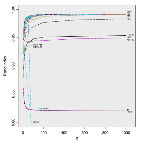
Figure 1: Rand index versus sample size $n$ (average across 100 replications).

Running time. The running times of the algorithms are displayed in Figure 2. During the simulations, algorithms were given 300 seconds to complete execution, after which they were interrupted. Accordingly any value 300s on the figure (often largely) underestimates the actual computation time. The algorithms can be divided in two groups: those who can solve (1) for $n=1000$ in 100s or far less, and those that time out (execution time over 300s) for $n\leq 500$ or far less. They are described below by order of decreasing speed.

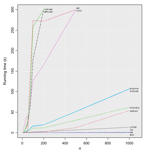
Figure 2: Running time versus sample size $n$ (average across 100 replications).

BCA, FW, and KM are the fastest methods with running times of order $10^{-3}$ to $10^{-1}$ seconds across values of $n$. For $n=1000$, they are one order of magnitude faster than the next best method (LCVQE). The HUB and REC initializations, although slower than arbitrary starting points like identity or random permutations, enable overall faster computations because good starting points reduce the number of iterations required for the main algorithm to converge. Completion of (100 runs) of BCA, FW, or FW based on the R100 initialization takes between 200 and 250 times the execution of a single run based on HUB or REC (instead of roughly 100). This is because the latter heuristics find good starting points whereas some (or many) of the 100 random starting points will be bad and require many iterations for the main algorithm to converge. KUR-ILP enjoys the same speed as the BCA, FW, and KM for small $n$ but its running time appears to scale polynomially with $n$. LCVQE appears to scale linearly with $n$ but with a much larger multiplicative constant than BCA, FW, and KM. Its running time is of order $10^{-2}$s for $n=5$ and 1s for $n=75$. The running time of CCLS grows steeply with $n$ and exceeds the 300s limit for $n\geq 500$. MPC-KM, COP-KM and EM are very slow, at least in their R implementation, and they time out (i.e. their execution times exceed 300s) for $n\geq 200$. Their computational load seems to grow exponentially with $n$. In the case of the EM, the computational bottleneck is the evaluation of matrix permanents. ILP, KUR-IQP and 2X are by far the slowest methods in the simulations. The first two stall and time out as soon as $n$ exceeds a few units, although they produce good results when $n\leq 5$. The computational load of 2X scales exponentially with $n$ (average computation time 110s for $n=30$); it is much higher when using the ID, R100, REC, and HUB initializations than when applied as a post-processing step following, say, the BCA method.

Summary of simulations.

• BCA is the fastest and most accurate of all studied methods. It provides excellent accuracy when initialized with REC or HUB. For best accuracy, the R100 initialization should be used at the cost of increased yet still manageable computations.

• BCA, KM, and FW are overall extremely fast and can handle datasets of size $n=10^{3}$ and up without difficulty. KM and FW are slightly less accurate than BCA in terms of optimization performance (relative error between $10^{-3}$ and $10^{-4}$) and Rand index.

• 2X is computationally costly and fairly inaccurate when used on its own, i.e. with an arbitrary starting point. It largely improves the accuracy of KM and FW solutions but not of BCA solutions. It is mostly beneficial in small to moderate dimension $n$.

• HUB and REC are not sufficiently accurate to be used on their own but they provide good starting points to more sophisticated matching methods. HUB uses data more extensively than REC and yields slightly better performance.

• For moderate to large $n$, EM shows poor performance in both computations (due to the evaluations of matrix permanents) and optimization. Its performance is satisfactory for $n\leq 50$, possibly because of the BCA initialization.

• ILP and KUR-BQP are only computationally feasible in very small samples ($n\leq 10$ or so). In this setup they virtually always find the global minimum of (1).

• KUR-ILP is relatively fast (it solves (1) for $n=1000$ in 50s) but not highly accurate (relative error between 3% and 5%). LCVQE is both faster and far less accurate: it solves (1) for $n=1000$ in 13s but has relative error in $(0.2,0.3)$ for all values of $n$.

• COP-KM and MPC-KM have very similar profiles in computation time and optimization accuracy. Their relative error goes from 0.2-0.3 for $n=5$ to 0.05-0.06 for $n=100$. They are not able to handle large datasets (at least not in their R implementation) as their computations stall for $n\geq 200$. CCLS only performs reasonably well for $n\leq 10$. Its Rand index and relative error deteriorate quickly as $n$ increases and its computations time out for $n\geq 500$.

4 Application to fMRI data

In this section we harness the matching problem (1) and its proposed solutions to analyze resting-state functional magnetic resonance imaging (rs-fMRI) data, the goal being to explore the dynamic functional connectivity (DFC) of the brain. In short, functional connectivity (FC) relates to the integration of brain activity, that is, how distant brain regions coordinate their activity to function as a whole. The dynamic nature of FC, in particular its dependence on factors such as task-related activity, psychological state, and cognitive processes, is well established in neuroimaging research (e.g. Chang and Glover, 2010; Handwerker et al., 2012; Hutchison et al., 2013).

The present analysis aims to extract measures of DFC from individual subject data and match these measures across subjects to uncover common patterns and salient features. The data under consideration are part of the ABIDE preprocessed data (Craddock et al., 2013), a large corpus of rs-fMRI measurements recorded from subjects diagnosed with autism spectrum disorder and from control subjects. These data and detailed descriptions are available at preprocessed-connectomes-project.org/abide/. We selected the following preprocessing options: Connectome Computation System (CCS) pipeline, spatial averaging over 116 regions of interest (ROI) defined by the AAL brain atlas, bandpass temporal filtering, no global signal regression. For simplicity, we only used data from control subjects and discarded data that did not not pass all quality control tests. This resulted in $n=308$ subjects with fMRI time series of average length about 200 scans (SD=62).

Subject-level analysis.

Vector autoregressive (VAR) models are widely used to assess FC in fMRI data (Valdés-Sosa et al., 2005; Friston et al., 2013; Ting et al., 2017). Here we represent the fMRI time series of a subject by a piecewise VAR model of order 1:

$$y_{t}=A_{t}y_{t-1}+b_{t}+\varepsilon_{t}\qquad(1\leq t\leq T)$$ (22)

where $y_{t}$ is an fMRI measurement vector of length 116, $A_{t}$ an unknown regression matrix encoding FC dynamics, $b_{t}$ an unknown baseline vector, and $\varepsilon_{t}$ a random noise vector with multivariate normal distribution $N(0,Q_{t})$. The $A_{t}$ are assumed sparse, reflecting the fact that only a small number of ROIs at time $t-1$ are predictive of ROI activity at time $t$. The model parameters $(A_{t},b_{t},Q_{t})$ are assumed piecewise constant with few change points, indicating that FC states persist for some time (say, between 5 and 50 scans) before the brain switches to a different FC state.

For each subject, the task at hand is to simultaneously detect change points in (22) and estimate $(A_{t},b_{t})$ over the associated time segments. ($Q_{t}$ is of secondary importance here and can be ignored). The sparse group fused lasso (SGFL) approach of Degras (2020) is designed for this purpose. To simplify the task of determining a suitable range for the SGFL regularization parameters and calculating regularization paths, we employ the two-step procedure of this paper. The first step detects change points via the group fused lasso (e.g. Bleakley and Vert, 2011); the second step recovers sparse estimates of the $A_{t}$ separately on each segment via the standard lasso (Tibshirani, 1996).

After fitting the regularization paths, a single lasso estimate $(\hat{A}_{t},\hat{b}_{t})$ is selected for each segment by the Akaike Information Criterion. Among all generated model segmentations, we retain the one with the most segments satisfying the following criteria: (i) length: the segment must have at least 5 scans, (ii) goodness of fit: the lasso fit must have a deviance ratio at least 0.3, and (iii) distinctness: the parameter estimate $\hat{A}_{t}$ for the segment must have at least 10% relative difference with estimates of other selected segments. To facilitate interpretation and remove noisy components, 10 segments are retained per subject at the most.

Group-level analysis.

Following the subject-level analysis, a set of change points and associated model parameter estimates is available for each subject, say $\{(\hat{A}_{ik},\hat{b}_{ik},\hat{T}_{ik}):1\leq k\leq m_{i}\}$ with $\hat{T}_{ik}$ the $k$th change point and $m_{i}$ the number of segments for the $i$th subject ($1\leq i\leq n$). The regression matrices $\hat{A}_{ik}$ provide informative FC measures and could in principle be used for group-level comparisons. They are however highly sparse and matching them using the squared Euclidean distance of problems (1)-(2) does not produce sensible results. We thus calculate the empirical correlation matrices on each segment $\{\hat{T}_{ik},\ldots,\hat{T}_{i(k+1)}-1\}$ and take them as inputs for the group analysis. See e.g. (Wang et al., 2014) for a review of common FC measures in neuroimaging. After discarding correlation matrices based on short segments (10 scans or less, for increased estimation accuracy) and extracting the lower halves of the remaining matrices, we obtain a set $\{x_{ik}:1\leq i\leq 306,1\leq k\leq m_{i}\}$ of 1801 correlation vectors of size $p=116\times 115/2=6670$. The number $m_{i}$ of vectors per subject varies in the range $[1,10]$ with an average of 5.88 (SD=1.77). The unbalanced matching problem (2) is then solved for $K\in\{10,20,\ldots,100\}$ using a generalized version of the BCA Algorithm 2. Based on the inspection of the cluster centers and cluster sizes, we retain the matching based on $K=100$ clusters. With this choice, cluster sizes are in the range $[12,28]$ (mean=18.01, SD=4.16). Smaller values of $K$, say $K\geq 50$, would be equally fine for data exploration. $K$ should however not be too small so as to avoid large clusters in which fine details of FC are averaged out in the cluster center and only large-scale features remain.

Figure 3 displays the 100 resulting cluster centers, i.e. the average correlation matrices of the clusters. For easier visualization and interpretation, the ROI-level correlations are aggregated into six well established resting state networks (RSN): the attentional network (26 ROIs), auditory network (6 ROIs), default mode network (32 ROIs), sensorimotor network (12 ROIs), subcortical network (8 ROIs), and visual network (14 ROIs). A list of the ROI names and associated RSNs is given in Appendix A. Note that some ROIs do not belong to any known functional networks while others are recruited in two networks. The visual network and auditory network have strong intracorrelation (0.59 and 0.64 on average across cluster centers, respectively, not including TPOsup in the auditory network). The subcortical network and sensorimotor network show moderate internal correlation (0.51 on average each). The default mode and attentional networks comprise more ROIs and are usually less correlated (0.36 and 0.40 on average, respectively). The hippocampus (HIP), parahippocampal gyrus (PHG), and amygdala (AMYG) cluster together fairly strongly (average correlation 0.53). Applying community detection algorithms to each cluster center with the R package igraph, we noticed that ROIs from the visual network are virtually always in the same community; the same holds true for the subcortical network. The strongest correlations found between RSNs are the following: auditory–sensorimotor (0.38 on average across clusters) attentional–default mode (0.36), attentional–sensorimotor (0.36), and sensorimotor–visual (0.35).

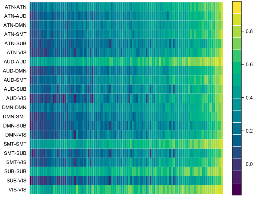
Figure 3: rs-fMRI data analysis. Each column represents the center of a cluster of matched features, that is, (half) a correlation matrix averaged across cluster members (subjects) and across ROIs of resting state networks. ATN: attentional network, AUD: auditory network, DMN: default mode network, SMT: sensorimotor network, SUB: subcortical network, VIS: visual network.

A remarkable feature (not visible in Figure 3) is the strong positive correlation between the Rolandic Operculum (ROL) and the regions PUT (subcortical network), PoCG, PreCG, and SMG (sensorimotor), and HES, STG (auditory) (between 0.42 and 0.67). In addition, CB9.R, VERMIS10, CB10.R, PCG.L, VERMIS9 exhibit consistent negative correlation (or at least lower average correlation) with most other ROIs. In particular, CB9.R (cerebellum) has 36.5% of negative correlations with other ROIs whereas the overall proportion of negative correlations in the 100 average correlation matrices is only 10.6%.

Figure 4 shows interesting examples of average correlation matrices (cluster centers) at the ROI level. Cluster 5 shows strong positive correlation within the auditory, subcortical, and visual networks, and in the small groups (HIP, PHG, AMYG), (CRUS1, CRUS2), and (CB3–CB6, VERMIS1–VERMIS7). ROL has moderate to strong negative correlation with CRUS1, CRUS2 and regions from the subcortical network (dark blue stripe towards the top and left) and strong positive correlation with PoCG, SMG (sensorimotor) and HES, STG (auditory). The auditory and sensorimotor networks have moderate to strong positive correlation. Cluster 14 shows clear blocking structure along the diagonal (correlation within RSN) as well as anticorrelation patterns between CAU, PUT, PAL, THA (subcortical) and ROL, PoCG (sensorimotor), PCL (sensorimotor); and between PCG (default mode) and PreCG (sensorimotor), ROL, PoCG (sensorimotor), PCL (sensorimotor). Community detection reveals three large and heterogeneous communities (sizes 43, 40, 36). Cluster 19 displays moderate to strong negative correlation (-0.55,-0.25) between IPL, SMG, ROL, CB10.R on the one hand and about 40 other ROIs on the other. The alternating clear and dark lines in cluster 27 reveal lateralized anticorrelation patterns between ROIs in the attentional network on the left side of the brain with most other ROIs in the brain. Cluster 42 shows two roughly uncorrelated blocks, a very large one with strong intracorrelation and a smaller one (CRUS, CB, VERMIS) with weaker intracorrelation. Cluster 88 displays a checkered correlation structure with strong anticorrelation between (CRUS, CB, VERMIS) and the rest of the brain.

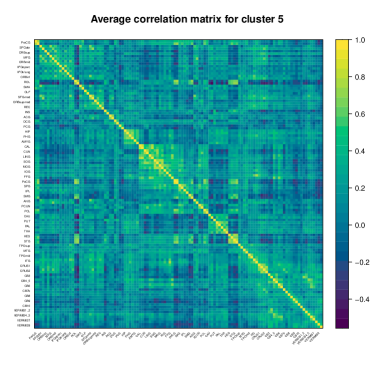
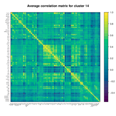
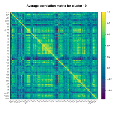
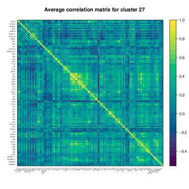
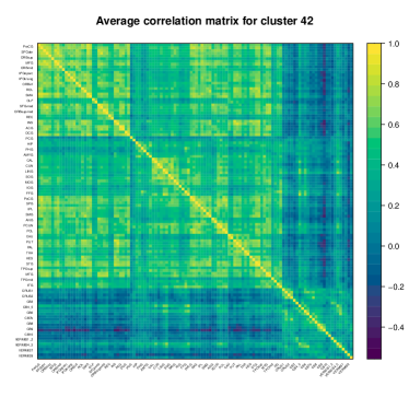
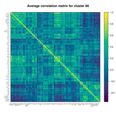
Figure 4: rs-fMRI data analysis. Examples of cluster centers (averages correlation matrices) derived from matching individual correlation matrices across subjects. Each displayed matrix corresponds to a cluster of 14 to 23 subjects.

Summary of the data analysis. The data analysis has established that the matching approach (1)-(2) provides scientifically meaningful insights into DFC at the group level. By inspecting the cluster centers (average correlation matrices) produced by the matching process, one recovers large-scale patterns consistent with neuroscientific knowledge. For example, known resting state networks are clearly reflected in the blocking structure of the cluster centers (see Figure 4). But the cluster centers can also generate new insights and hypotheses. For example, the Heschl gyrus (HES) is not systematically included in the auditory network but, according to our analysis, it should. Similarly, the ROI TPOsup (temporal lobe: superior temporal gyrus), although it is near to or part of the auditory cortex, has shown only weak correlation with the other ROI of the auditory network, Superior temporal gyrus (STG). These elements may lead to a more nuanced understanding of the auditory network. Other remarkable findings include the strong anticorrelations found between the Rolandic operculum (ROL), the cerebellum (CER) and the vermis (VERMIS) on the one hand and (a large part of) the rest of the brain on the other. Importantly, by design, each of the clusters formed by the matching process highlights commonalities between subjects and not within subjects. This is in contrast with unconstrained clustering methods (e.g. $K$-means clustering) whose clusters may consist in (vectors from) a small number of or even a single subject in extreme cases.

5 Discussion

We have sought to efficiently match feature vectors in a one-to-one fashion across large collections of datasets or statistical units. In applications where statistical units are matched in pairs, this task is conveniently framed as a multidimensional assignment problem with decomposable costs (MDAC). Taking the squared Euclidean distance as dissimilarity function in the MDADC enables tremendous computational speedup by transforming ${n\choose 2}$ related matching problems between all pairs of datasets into $n$ separate matching problems between each dataset and a template. Leveraging this idea, we have developed extremely fast algorithms whose computational complexity scales linearly with $n$. These algorithms do not require precalculating and storing assignment costs, which may be infeasible in large-scale applications. Instead, they efficiently calculate assignment costs on the fly. To our knowledge, no other available method to solve the MDADC possesses either of these linear scaling and storage-free properties necessary to large-scale applications.

Our proposed algorithms rely on various optimization techniques such as $K$-means clustering, block coordinate ascent (BCA), convex relaxation, the Frank-Wolfe algorithm, and pairwise interchange heuristic. We have also taken a probabilistic view of (1) leading to a constrained Gaussian mixture model and associated EM algorithm. Altogether the proposed algorithms form a panel that covers most types of approach to the MDADC found in the literature. (As discussed earlier, we have not considered Lagrangian relaxation methods as they require computer clusters and/or GPUs for efficient large-scale implementation.) These algorithms extend or specialize existing approaches in a nontrivial way. For example, the BCA and 2-exchange algorithms, which are specialized versions of existing algorithms, scale linearly with $n$ and are amenable to large-scale applications whereas the more general algorithms are not.

The numerical study has shown the excellent performances of the three main algorithms: $K$-means matching, BCA, and Frank-Wolfe, with respect to computation and optimization. In particular, these algorithms largely outperform all competitors and can handle very large collections of data. The BCA algorithm shows slightly better performance than the other two. The pairwise interchange heuristic can enhance these two methods to reach near optimality at a hefty computational price. The EM algorithm displayed fairly poor performance throughout the study. Upon inspection, the poor optimization results came from the fact that the algorithm was “too sure” about the allocation probabilities (of data vectors to classes) which were almost invariably calculated as 0 or 1. This in turn may arise from the (relatively) high dimension of the data, short tails of the normal distribution, and/or error in covariance estimation. Using the deterministic annealing EM and/or random starting points did not fix the issue. Solutions for improving the EM optimization may be to impose a diagonal structure on covariance estimates or to consider (mixtures of) distributions with heavier tails such as multivariate $t$-distributions. The computational slowness of the EM could be remedied by calculating a small fixed number of most likely allocations rather than computing them all through matrix permanents.

The analysis of the ABIDE preprocessed fMRI data has shown the strong potential of the proposed feature matching approach for exploring neuroimaging biomarkers and producing interpretable clusters at the group level. A key characteristic of one-to-one feature matching is that, unlike unsupervised clustering, it is guaranteed to produce “representative” clusters that reflect variations between subjects and not within. While feature matching was employed in our analysis for data exploration, this technique could also be used in a more principled way as a preliminary step to disentangle association ambiguities between biomarkers and/or to stratify subjects into small, homogenous groups prior to a group-level analysis. Such matching-based approach could be for example compared to the consensus clustering strategy of Rasero et al. (2019).

Possible extensions and future work.

• Weighted (squared) Euclidean distance. The squared Euclidean distance in (1) can easily be generalized to a weighted squared Euclidean distance $\|x\|_{W}^{2}=x^{\prime}Wx$ with $W\in\mathbb{R}^{p\times p}$ a positive semi-definite matrix. Decomposing $W$ as $L^{\prime}L$ (e.g. by Cholesky decomposition), it suffices to premultiply each matrix $X_{i}$ by $L$ to formulate an equivalent problem (1) using the unweighted (squared) Euclidean distance.

• Alternative dissimilarity measures. Although the squared Euclidean distance for $d$ in the general MDADC problem (3)-(4) enables extremely fast and scalable algorithms with low memory footprint, it may not adequately capture relevant differences between feature vectors in some applications. If the Euclidean distance $\|\cdot\|_{2}$ or the Manhattan distance $\|\cdot\|_{1}$, for example, is a more sensible choice for $d$, a reasonable approach would be to use an objective function based on the ($nm$) distances between feature vectors and their cluster centers instead of one based on the distances between all ${n\choose 2}m$ pairs of matched vectors. In this case, the $K$-means matching Algorithm 1 can be adapted as follows. The assignment step remains the same: given cluster centers $c_{1},\ldots,c_{m}$, the feature vectors of each unit $i\in[n]$ are assigned to clusters by minimizing the LAP with assignment matrix $A_{i}=(d(x_{ik},c_{l}))_{1\leq k,l\leq m}$. The updating step for the cluster centers proceeds from calculating $m$ geometric medians if $d=\|\cdot\|_{2}$, or $mp$ univariate medians id $d=\|\cdot\|_{1}$. Both these tasks can be accomplished in near linear time, and like in the case $d=\|\cdot\|_{2}^{2}$, no distance needs to be pre-calculated and stored. Accordingly, the modified objective function and modified $K$-means matching algorithm still enable linear time complexity linear in $n$ and low space requirements. (The other algorithms of Section 2 do not extend quite so nicely as they fundamentally rely on the scalar product and separability properties that underlie $\|\cdot\|_{2}^{2}$.)

• Gaining theoretical understanding of the optimization properties of the algorithms of this paper, for example by establishing deterministic or probabilistic bounds on their performances, could maybe explain the very good performances observed and/or give insights on worst case performance in difficult instances (e.g. Gutin et al., 2008). Also, obtaining tight lower bounds through suitable Lagrangian relaxations would be desirable in practice.

• The rich structure of problem (1) may make it possible to easily construct instances in which the global minimum and optimal assignment are known (see e.g. Drugan, 2015, for related work on quadratic assignment problems). This would be of course useful to benchmark methods.

Acknowledgments

The author thanks to Vince Lyzinski for early discussions that led to the convex relaxation/
Frank-Wolfe approach of Section 2.3. He also acknowledges his student Yiming Chen for his assistance in the literature search and the numerical study.

Appendix A Brain regions of interest in fMRI data analysis

Label	Name	Abbrv	Label	Name	Abbrv
	Subcortical network			Default mode network
71	L Caudate nucleus	CAU.L	5	L Superior frontal gyrus, orbital	ORBsup.L
72	R Caudate nucleus	CAU.R	6	R Superior frontal gyrus, orbital	ORBsup.R
73	L Putamen	PUT.L	7	L Middle frontal gyrus	MFG.L
74	R Putamen	PUT.R	8	R Middle frontal gyrus	MFG.R
75	L Pallidum	PAL.L	15	L Inferior frontal gyrus, orbital	ORBinf.L
76	R Pallidum	PAL.R	16	R Inferior frontal gyrus, orbital	ORBinf.R
77	L Thalamus	THA.L	23	L Superior frontal gyrus, medial	SFGmed.L
78	R Thalamus	THA.R	24	R Superior frontal gyrus, medial	SFGmed.R
	Auditory network		25	L Superior frontal gyrus, medial orbital	ORBsupmed.L
79	L Heschl gyrus	HES.L	26	R Superior frontal gyrus, medial orbital	ORBsupmed.R
80	R Heschl gyrus	HES.R	31	L Cingulate gyrus, anterior part	ACG.L
81	L Superior temporal gyrus	STG.L	32	R Cingulate gyrus, anterior part	ACG.R
82	R Superior temporal gyrus	STG.R	33	L Cingulate gyrus, mid part	DCG.L
83	L Temporal pole: superior temporal gyrus	TPOsup.L	34	R Cingulate gyrus, mid part	DCG.R
84	R Temporal pole: superior temporal gyrus	TPOsup.R	35	L Cingulate gyurs, posterior part	PCG.L
	Sensorimotor network		36	R Cingulate gyrus, posterior part	PCG.R
1	L Precentral gyrus	PreCG.L	37	L Hippocampus	HIP.L
2	R Precentral gyrus	PreCG.R	38	R Hippocampus	HIP.R
19	L Supplementary motor area	SMA.L	39	L Parahippocampus	PHG.L
20	R Supplementary motor area	SMA.R	40	R Parahippocampus	PHG.R
57	L Postcentral gyrus	PoCG.L	61	L Inferior parietal gyrus	IPL.L
58	R Postcentral gyrus	PoCG.R	62	R Inferior parietal gyrus	IPL.R
59	L Superior parietal gyrus	SPG.L	65	L Angular gyrus	ANG.L
60	R Superior parietal gyrus	SPG.R	66	R Angular gyrus	ANG.R
63	L Supramarginal gyrus	SMG.L	67	L Precuneus	PCUN.L
64	R Supramarginal gyrus	SMG.R	68	R Precuneus	PCUN.R
69	L Paracentral lobule	PCL.L	85	L Middle temporal gyrus	MTG.L
70	R Paracentral lobule	PCL.R	86	R Middle temporal gyrus	MTG.R
	Visual network		87	L Temporal pole: middle temporal gyrus	TPOmid.L
43	L Calcarine fissure and surrounding cortex	CAL.L	88	R Temporal pole: middle temporal gyrus	TPOmid.R
44	R Calcarine fissure and surrounding cortex	CAL.R	89	L Inferior temporal gyrus	ITG.L
45	L Cuneus	CUN.L	90	R Inferior temporal gyrus	ITG.R
46	R Cuneus	CUN.R		Unclassified
47	L Lingual gyrus	LING.L	17	L Rolandic operculum	ROL.L
48	R Lingual gyrus	LING.R	18	R Rolandic operculum	ROL.R
49	L Superior occipital lobe	SOG.L	21	L Olfactory cortex	OLF.L
50	R Superior occipital lobe	SOG.R	22	R Olfactory cortex	OLF.R
51	L Middle occipital lobe	MOG.L	27	L Gyrus rectus	REC.L
52	R Middle occipital lobe	MOG.R	28	R Gyrus rectus	REC.R
53	L Inferior occipital lobe	IOG.L	41	L Amygdala	AMYG.L
54	R Inferior occipital lobe	IOG.R	42	R Amygdala	AMYG.R
55	L Fusiform gyrus	FFG.L	91	L Cerebellum crus 1	CRUS1.L
56	R Fusiform gyrus	FFG.R	92	R Cerebellum crus 1	CRUS1.R
	Attentional network		93	L Cerebellum crus 2	CRUS2.L
3	L Superior frontal gyrus, dorsolateral	SFGdor.L	94	R Cerebellum crus 2	CRUS2.R
4	R Superior frontal gyrus, dorsolateral	SFGdor.R	95	L Cerebellum 3	CB3.L
5	L Superior frontal gyrus, orbital	ORBsup.L	96	R Cerebellum 3	CB3.R
6	R Superior frontal gyrus, orbital	ORBsup.R	97	L Cerebellum 4 5	CB4_5.L
7	L Middle frontal gyrus	MFG.L	98	R Cerebellum 4 5	CB4_5.R
8	R Middle frontal gyrus	MFG.R	99	L Cerebellum 6	CB6.L
9	L Middle frontal gyrus, orbital	ORBmid.L	100	R Cerebellum 6	CB6.R
10	R Middle frontal gyrus, orbital	ORBmid.R	101	L Cerebellum 7	CB7b.L
11	L Inferior frontal gyrus, opercular	IFGoperc.L	102	R Cerebellum 7	CB7b.R
12	R Inferior frontal gyrus, opercular	IFGoperc.R	103	L Cerebellum 8	CB8.L
13	L Inferior frontal gyrus, triangular	IFGtriang.L	104	R Cerebellum 8	CB8.R
14	R Inferior frontal gyrus, triangular	IFGtriang.R	105	L Cerebellum 9	CB9.L
15	L Inferior frontal gyrus, orbital	ORBinf.L	106	R Cerebellum 9	CB9.R
16	R Inferior frontal gyrus, orbital	ORBinf.R	107	L Cerebellum 10	CB10.L
29	L Insula	INS.L	108	R Cerebellum 10	CB10.R
30	R Insula	INS.R	109	Vermis 12	VERMIS1_2
59	L Superior parietal gyrus	SPG.L	110	Vermis 3	VERMIS3
60	R Superior parietal gyrus	SPG.R	111	Vermis 4 5	VERMIS4_5
61	L Inferior parietal gyrus	IPL.L	112	Vermis 6	VERMIS6
62	R Inferior parietal gyrus	IPL.R	113	Vermis 7	VERMIS7
83	L Temporal pole: superior temporal gyrus	TPOsup.L	114	Vermis 8	VERMIS8
84	R Temporal pole: superior temporal gyrus	TPOsup.R	115	Vermis 9	VERMIS9
85	L Middle temporal gyrus	MTG.L	116	Vermis 10	VERMIS10
86	R Middle temporal gyrus	MTG.R
89	L Inferior temporal gyrus	ITG.L
90	R Inferior temporal gyrus	ITG.R

Table 2: rs-fMRI data analysis. Regions of interest (ROIs) as defined by the AAL brain atlas and resting state networks (RSN).

References

- Ashburner [2007] John Ashburner. A fast diffeomorphic image registration algorithm. NeuroImage, 38(1):95 – 113, 2007.
- Balas and Saltzman [1991] Egon Balas and Matthew J. Saltzman. An algorithm for the three-index assignment problem. Oper. Res., 39(1):150–161, 1991.
- Bandelt et al. [2004] H.-J. Bandelt, A. Maas, and F. C. R. Spieksma. Local search heuristics for multi-index assignment problems with decomposable costs. J. Oper. Res. Soc., 55(7):694–704, 2004.
- Bandelt et al. [1994] Hans-Jürgen Bandelt, Yves Crama, and Frits C. R. Spieksma. Approximation algorithms for multi-dimensional assignment problems with decomposable costs. Discrete Appl. Math., 49(1-3):25–50, 1994.
- Bar-Shalom et al. [2011] Y. Bar-Shalom, P.K. Willett, and X. Tian. Tracking and Data Fusion: A Handbook of Algorithms. YBS Publishing, 2011.
- Basu et al. [2009] Sugato Basu, Ian Davidson, and Kiri L. Wagstaff, editors. Constrained clustering: Advances in algorithms, theory, and applications. Chapman & Hall/CRC Data Mining and Knowledge Discovery Series. CRC Press, 2009.
- Belongie et al. [2002] S. Belongie, J. Malik, and J. Puzicha. Shape matching and object recognition using shape contexts. IEEE Trans. Pattern Anal. Mach. Intell., 24(4):509–522, 2002.
- Bilenko et al. [2004] Mikhail Bilenko, Sugato Basu, and Raymond J. Mooney. Integrating constraints and metric learning in semi-supervised clustering. In Machine Learning, Proceedings of the Twenty-first International Conference (ICML 2004), volume 69. ACM, 2004.
- Birkhoff [1946] Garrett Birkhoff. Tres observaciones sobre el algebra lineal [Three observations on linear algebra]. Univ. Nac. Tucumán. Revista A., 5:147–151, 1946.
- Bleakley and Vert [2011] Kevin Bleakley and Jean-Philippe Vert. The group fused lasso for multiple change-point detection. Technical Report hal-00602121, 2011.
- Burkard et al. [2009] Rainer Burkard, Mauro Dell’Amico, and Silvano Martello. Assignment problems. Society for Industrial and Applied Mathematics (SIAM), Philadelphia, PA, 2009.
- Çela [1998] Eranda Çela. The quadratic assignment problem, volume 1 of Combinatorial Optimization. Kluwer Academic Publishers, Dordrecht, 1998.
- Chang and Glover [2010] C. Chang and G. H. Glover. Time-frequency dynamics of resting-state brain connectivity measured with fMRI. Neuroimage, 50(1):81–98, Mar 2010.
- Collier and Dalalyan [2016] Olivier Collier and Arnak S. Dalalyan. Minimax rates in permutation estimation for feature matching. J. Mach. Learn. Res., 17(6):1–31, 2016.
- Collins [2012] Robert T. Collins. Multitarget data association with higher-order motion models. In 2012 IEEE Conference on Computer Vision and Pattern Recognition, pages 1744–1751, 2012.
- Conte et al. [2004] D. Conte, P. Foggia, C. Sansone, and M. Vento. Thirty years of graph matching in pattern recognition. Int. J. Pattern Recognit. Artif. Intell., 18:265–298, 2004.
- Craddock et al. [2013] Cameron Craddock, Yassine Benhajali, Carlton Chu, Francois Chouinard, Alan Evans, András Jakab, Budhachandra Khundrakpam, John Lewis, Qingyang Li, Michael Milham, Chaogan Yan, and Pierre Bellec. The neuro bureau preprocessing initiative: open sharing of preprocessed neuroimaging data and derivatives. Frontiers in Neuroinformatics, 7, 2013.
- Degras [2020] David Degras. Sparse group fused lasso for model segmentation: a hybrid approach. Adv. Data Anal. Classif., 2020. doi: https://doi.org/10.1007/s11634-020-00424-5.
- DeGroot and Goel [1976] Morris H. DeGroot and Prem K. Goel. The matching problem for multivariate normal data. Sankhyā Ser. B, 38(1):14–29, 1976.
- Dehghan et al. [2015] A. Dehghan, S. M. Assari, and M. Shah. GMMCP tracker: Globally optimal generalized maximum multi clique problem for multiple object tracking. In 2015 IEEE Conference on Computer Vision and Pattern Recognition (CVPR), pages 4091–4099, 2015.
- Doherty et al. [2019] K. Doherty, D. Fourie, and J. Leonard. Multimodal semantic SLAM with probabilistic data association. In 2019 International Conference on Robotics and Automation (ICRA), pages 2419–2425, 2019.
- Drugan [2015] Mădălina M. Drugan. Generating QAP instances with known optimum solution and additively decomposable cost function. J. Comb. Optim., 30(4):1138–1172, 2015.
- Frank and Wolfe [1956] Marguerite Frank and Philip Wolfe. An algorithm for quadratic programming. Naval Research Logistics Quarterly, 3(1?2):95–110, 1956.
- Friston et al. [2013] Karl Friston, Rosalyn Moran, and Anil K Seth. Analysing connectivity with granger causality and dynamic causal modelling. Current Opinion in Neurobiology, 23(2):172 – 178, 2013. Macrocircuits.
- Gancarski et al. [2020] P. Gancarski, T-B-H. Dao, B. Crémilleux, G. Forestier, and T. Lampert. Constrained clustering: Current and new trends. In A Guided Tour of AI Research, pages 447–484. Springer, 2020.
- Gutin et al. [2008] Gregory Gutin, Boris Goldengorin, and Jing Huang. Worst case analysis of max-regret, greedy and other heuristics for multidimensional assignment and traveling salesman problems. Journal of heuristics, 14(2):169–181, 2008.
- Handwerker et al. [2012] D. A. Handwerker, V. Roopchansingh, J. Gonzalez-Castillo, and P. A. Bandettini. Periodic changes in fMRI connectivity. Neuroimage, 63(3):1712–1719, Nov 2012.
- Haxby et al. [2011] James V. Haxby, J. Swaroop Guntupalli, Andrew C. Connolly, Yaroslav O. Halchenko, Bryan R. Conroy, M. Ida Gobbini, Michael Hanke, and Peter J. Ramadge. A common, high-dimensional model of the representational space in human ventral temporal cortex. Neuron, 72(2):404–416, 2011.
- Hiep et al. [2016] Tran Khanh Hiep, Nguyen Minh Duc, and Bui Quoc Trung. Local search approach for the pairwise constrained clustering problem. In Proceedings of the Seventh Symposium on Information and Communication Technology, SoICT ’16, pages 115–122. ACM, 2016.
- Hsu et al. [2017] Daniel Hsu, Kevin Shi, and Xiaorui Sun. Linear regression without correspondence. In Advances in Neural Information Processing Systems, volume 30, pages 1531–1540. Curran Associates, Inc., 2017.
- Hutchison et al. [2013] R. M. Hutchison, T. Womelsdorf, E. A. Allen, P. A. Bandettini, V. D. Calhoun, M. Corbetta, S. Della Penna, J. H. Duyn, G. H. Glover, J. Gonzalez-Castillo, D. A. Handwerker, S. Keilholz, V. Kiviniemi, D. A. Leopold, F. de Pasquale, O. Sporns, M. Walter, and C. Chang. Dynamic functional connectivity: promise, issues, and interpretations. Neuroimage, 80:360–378, Oct 2013.
- Jerrum et al. [2004] Mark Jerrum, Alistair Sinclair, and Eric Vigoda. A polynomial-time approximation algorithm for the permanent of a matrix with nonnegative entries. J. ACM, 51(4):671–697, 2004.
- Karapetyan and Gutin [2011] Daniel Karapetyan and Gregory Gutin. Local search heuristics for the multidimensional assignment problem. Journal of Heuristics, 17(3):201–249, 2011.
- Kochenberger et al. [2014] Gary Kochenberger, Jin-Kao Hao, Fred Glover, Mark Lewis, Zhipeng Lü, Haibo Wang, and Yang Wang. The unconstrained binary quadratic programming problem: a survey. J. Comb. Optim., 28(1):58–81, 2014.
- Koopmans and Beckmann [1957] Tjalling C. Koopmans and Martin Beckmann. Assignment problems and the location of economic activities. Econometrica, 25:53–76, 1957.
- Kuck et al. [2019] Jonathan Kuck, Tri Dao, Hamid Rezatofighi, Ashish Sabharwal, and Stefano Ermon. Approximating the permanent by sampling from adaptive partitions. In Advances in Neural Information Processing Systems, volume 32, pages 8860–8871. Curran Associates, Inc., 2019.
- Kuhn [1955] H. W. Kuhn. The Hungarian method for the assignment problem. Naval Research Logistics Quarterly, 2(1-2):83–97, 1955.
- Kuroki and Matsui [2009] Yusuke Kuroki and Tomomi Matsui. An approximation algorithm for multidimensional assignment problems minimizing the sum of squared errors. Discrete Appl. Math., 157(9):2124–2135, 2009.
- Le Moigne et al. [2011] J. Le Moigne, N.S. Netanyahu, and R.D. Eastman. Image Registration for Remote Sensing. Cambridge University Press, 2011.
- Lloyd [1982] Stuart P. Lloyd. Least squares quantization in PCM. IEEE Trans. Inform. Theory, 28(2):129–137, 1982.
- Lowe [2001] D.G Lowe. Local feature view clustering for 3D object recognition. In Proceedings of the 2001 IEEE Computer Society Conference on Computer Vision and Pattern Recognition. CVPR 2001, volume 1, pages I–I, 2001.
- Lyzinski et al. [2016] V. Lyzinski, D. E. Fishkind, M. Fiori, J. T. Vogelstein, C. E. Priebe, and G. Sapiro. Graph matching: Relax at your own risk. IEEE Trans. Pattern Anal. Mach. Intell., 38(1):60–73, 2016.
- McLachlan and Peel [2000] Geoffrey McLachlan and David Peel. Finite mixture models. Wiley Series in Probability and Statistics: Applied Probability and Statistics. Wiley-Interscience, New York, 2000.
- McLachlan and Krishnan [2008] Geoffrey J. McLachlan and Thriyambakam Krishnan. The EM algorithm and extensions. Wiley-Interscience [John Wiley & Sons], Hoboken, NJ, second edition, 2008.
- Munkres [1957] James Munkres. Algorithms for the assignment and transportation problems. J. Soc. Indust. Appl. Math., 5:32–38, 1957.
- Natu et al. [2020] Shardul Natu, Ketan Date, and Rakesh Nagi. GPU-accelerated Lagrangian heuristic for multidimensional assignment problems with decomposable costs. Parallel Computing, page 102666, 2020.
- Nijenhuis and Wilf [1978] Albert Nijenhuis and Herbert S. Wilf. Combinatorial algorithms. Academic Press, Inc., second edition, 1978.
- Oliveira and Pardalos [2004] Carlos A. S. Oliveira and Panos M. Pardalos. Randomized parallel algorithms for the multidimensional assignment problem. Appl. Numer. Math., 49(1):117–133, 2004. doi: 10.1016/j.apnum.2003.11.014.
- Pananjady et al. [2018] A. Pananjady, M. J. Wainwright, and T. A. Courtade. Linear regression with shuffled data: Statistical and computational limits of permutation recovery. IEEE Transactions on Information Theory, 64(5):3286–3300, 2018.
- Pardalos and Pitsoulis [2000] Panos M. Pardalos and Leonidas S. Pitsoulis, editors. Nonlinear assignment problems, volume 7 of Combinatorial Optimization. Kluwer Academic Publishers, Dordrecht, 2000.
- Pelleg and Baras [2007] Dan Pelleg and Dorit Baras. K -means with large and noisy constraint sets. In ECML 2007, pages 674–682. Springer, 2007.
- Pierskalla [1968] William P. Pierskalla. The multidimensional assignment problem. Operations Research, 16(2):422–431, 1968.
- Poore and Rijavec [1993] Aubrey P. Poore and Nenad Rijavec. A Lagrangian relaxation algorithm for multidimensional assignment problems arising from multitarget tracking. SIAM J. Optim., 3(3):544–563, 1993.
- Press et al. [2007] William H. Press, Saul A. Teukolsky, William T. Vetterling, and Brian P. Flannery. Numerical Recipes 3rd Edition: The Art of Scientific Computing. Cambridge University Press, 2007.
- Qiao and Li [2015] Mu Qiao and Jia Li. Gaussian mixture models with component means constrained in pre-selected subspaces, 2015.
- Rand [1971] William M. Rand. Objective criteria for the evaluation of clustering methods. J. Amer. Statist. Assoc., 66(336):846–850, 1971.
- Rasero et al. [2019] Javier Rasero, Ibai Diez, Jesus M. Cortes, Daniele Marinazzo, and Sebastiano Stramaglia. Connectome sorting by consensus clustering increases separability in group neuroimaging studies. Network Neuroscience, 3(2):325–343, 2019.
- Rezatofighi et al. [2015] S. H. Rezatofighi, A. Milan, Z. Zhang, Q. Shi, A. Dick, and I. Reid. Joint probabilistic data association revisited. In 2015 IEEE International Conference on Computer Vision (ICCV), pages 3047–3055, 2015.
- Robertson [2001] Alexander J. Robertson. A set of greedy randomized adaptive local search procedure (GRASP) implementations for the multidimensional assignment problem. Computational Optimization and Applications, 19(2):145–164, 2001.
- Ryser [1963] Herbert J. Ryser. Combinatorial mathematics, volume 14 of The Carus Mathematical Monographs. Wiley and Sons, Inc., New York, 1963.
- Shalom et al. [2010] Mordechai Shalom, Prudence W. H. Wong, and Shmuel Zaks. On-line maximum matching in complete multipartite graphs with implications to the minimum ADM problem on a star topology. In Structural information and communication complexity, volume 5869 of Lecture Notes in Comput. Sci., pages 281–294. Springer, Berlin, 2010.
- Shental et al. [2004] Noam Shental, Aharon Bar-hillel, Tomer Hertz, and Daphna Weinshall. Computing gaussian mixture models with EM using equivalence constraints. In Advances in Neural Information Processing Systems, volume 16, pages 465–472. MIT Press, 2004.
- Sinkhorn [1964] Richard Sinkhorn. A relationship between arbitrary positive matrices and doubly stochastic matrices. Ann. Math. Statist., 35:876–879, 1964.
- Smeulders et al. [2014] A. W. M. Smeulders, D. M. Chu, R. Cucchiara, S. Calderara, A. Dehghan, and M. Shah. Visual tracking: An experimental survey. IEEE Trans. Pattern Anal. Mach. Intell., 36(7):1442–1468, 2014.
- Spieksma and Woeginger [1996] F.C.R. Spieksma and G.J. Woeginger. Geometric three-dimensional assignment problems. European Journal of Operational Research, 91(3):611–618, 1996.
- Tauer and Nagi [2013] Gregory Tauer and Rakesh Nagi. A map-reduce Lagrangian heuristic for multidimensional assignment problems with decomposable costs. Parallel Computing, 39(11):653 – 668, 2013.
- Thornbrue et al. [2010] James R. Thornbrue, J. Nate Knight, and Benjamin J. Slocumb. Association ambiguity management in mixed data dimension tracking problems. In Signal and Data Processing of Small Targets 2010, volume 7698, pages 255–266. International Society for Optics and Photonics, SPIE, 2010.
- Tibshirani [1996] Robert Tibshirani. Regression shrinkage and selection via the lasso. J. Roy. Statist. Soc. Ser. B, 58(1):267–288, 1996.
- Ting et al. [2017] C. M. Ting, H. Ombao, S. B. Samdin, and S. H. Salleh. Estimating dynamic connectivity states in fMRI using regime-switching factor models. IEEE Transactions on Medical Imaging, PP(99):1–1, 2017. ISSN 0278-0062.
- Ueda and Nakano [1998] Naonori Ueda and Ryohei Nakano. Deterministic annealing EM algorithm. Neural Netw., 11(2):271–282, 1998.
- Uhlmann [2004] Jeffrey K. Uhlmann. Matrix permanent inequalities for approximating joint assignment matrices in tracking systems. J. Franklin Inst., 341(7):569–593, 2004.
- Valdés-Sosa et al. [2005] Pedro A. Valdés-Sosa, Jose M. Sánchez-Bornot, Agustín Lage-Castellanos, Mayrim Vega-Hernández, Jorge Bosch-Bayard, Lester Melie-García, and Erick Canales-Rodríguez. Estimating brain functional connectivity with sparse multivariate autoregression. Philosophical Transactions: Biological Sciences, 360(1457):969–981, 2005.
- Vogelstein et al. [2015] Joshua T. Vogelstein, John M. Conroy, Vince Lyzinski, Louis J. Podrazik, Steven G. Kratzer, Eric T. Harley, Donniell E. Fishkind, R. Jacob Vogelstein, and Carey E. Priebe. Fast approximate quadratic programming for graph matching. PLOS ONE, 10(4):1–17, 04 2015.
- von Neumann [1953] John von Neumann. A certain zero-sum two-person game equivalent to the optimal assignment problem. In Contributions to the theory of games, vol. 2, Annals of Mathematics Studies, no. 28, pages 5–12. Princeton University Press, Princeton, N. J., 1953.
- Wagstaff et al. [2001] Kiri Wagstaff, Claire Cardie, Seth Rogers, and Stefan Schrödl. Constrained -means clustering with background knowledge. In ICML ’01, pages 577–584, San Francisco, CA, USA, 2001. Morgan Kaufmann Publishers Inc.
- Wang et al. [2014] H. E. Wang, C. G. Benar, P. P. Quilichini, K. J. Friston, V. K. Jirsa, and C. Bernard. A systematic framework for functional connectivity measures. Front. Neurosci., 8:405, 2014.
- Wang et al. [2015] L. Wang, T. Liu, G. Wang, K. L. Chan, and Q. Yang. Video tracking using learned hierarchical features. IEEE Trans. Image Proc., 24(4):1424–1435, 2015.
- Wright [2015] Stephen J. Wright. Coordinate descent algorithms. Math. Program., 151(1, Ser. B):3–34, 2015.