Deep Reinforcement Learning with Quantum-inspired Experience Replay

Abstract

In this paper, a novel training paradigm inspired by quantum computation is proposed for deep reinforcement learning (DRL) with experience replay. In contrast to traditional experience replay mechanism in DRL, the proposed deep reinforcement learning with quantum-inspired experience replay (DRL-QER) adaptively chooses experiences from the replay buffer according to the complexity and the replayed times of each experience (also called transition), to achieve a balance between exploration and exploitation. In DRL-QER, transitions are first formulated in quantum representations, and then the preparation operation and the depreciation operation are performed on the transitions. In this progress, the preparation operation reflects the relationship between the temporal difference errors (TD-errors) and the importance of the experiences, while the depreciation operation is taken into account to ensure the diversity of the transitions. The experimental results on Atari 2600 games show that DRL-QER outperforms state-of-the-art algorithms such as DRL-PER and DCRL on most of these games with improved training efficiency, and is also applicable to such memory-based DRL approaches as double network and dueling network.

I Introduction

Reinforcement learning (RL) is an intelligent paradigm that learns through the interaction with the environment. During the training process of this interaction-based algorithm, similar to human behaviours [1, 2, 3], the agent adjusts its behavior to maximize the cumulative rewards for the entire control task according to the retroaction it receives from the environment. When it comes to the general situation of the real world environment, most control tasks often come with high-dimensional inputs, where traditional RL approaches cannot work well. Fortunately, deep learning provides a new approach to handle the complex input information and has achieved huge breakthrough in various fields [4, 5, 6, 7, 8, 9, 10]. In particular, by combining deep learning with RL, a new framework of deep reinforcement learning (DRL) arises, where Deep Q Network (DQN) becomes one of the most famous DRL methods [11].

DQN was employed to estimate the action values to help the agent make sequential decisions, where raw images were fed into the convolutional neural networks followed by the fully connected networks to output the action values that estimated the future rewards. In order to improve the utilization of the state-action transitions, an experience replay mechanism was deployed in the DQN framework [12], where experiences were stored in a finite-size buffer and were retrieved from the buffer. This mechanism of experience replay effectively sped up the processing of the experiences during training, but it ignored the difference in the importance between experiences. A series of experience replay variants have been developed to further improve the learning process, such as prioritized experience replay (PER) [13], deep curriculum reinforcement learning (DCRL) [14], remember and forget for experience replay (ReF-ER) [15], attentive experience replay (AER) [16] and competitive experience replay (CER) [17].

In PER, temporal difference errors (TD-errors) determine the priorities of the experiences and influence the probabilities of those experiences’ being replayed. This method further enhance the utilization of experiences compared to the original experience replay, but the data generated by the agent are noisy. Since DRL-PER gives higher priorities to transitions with larger TD errors and there might exist some experiences whose large TD-errors would not decrease even after many times of replay. From this respective, DRL-PER may cause some experiences to be overused, which might result in oscillations of the neural network [18]. To improve the sample efficiency of DQN, DCRL proposed a criterion for the samples’ importance based on the difficulties and the diversities of the experiences, where the difficulties are positively correlated with TD-errors and the diversities are related to the number of replaying times [14]. However, it introduced a number of parameters that required more prior knowledge to tune accurately. In ReF-ER [15], policy updates are penalized according to Kullback-Leibler divergence to accelerate convergence, attentive experience replay (AER) selects experiences according to the similarities between their states and the agent’s current state [16] and CER sets up two agents for competitive exploration between a pair of agents [17]. But these three methods may rely on high computing resources. Hence, it is desirable to design a more effective and general approach to enhance the experience replaying method for DRL.

At the same time, quantum physics have been employed to dramatically enhance information processing capability [19, 20, 21, 22, 23, 24, 25, 26] and have a positive influence on specific algorithmic tasks of applied artificial intelligence [27, 28, 29, 30]. In particular, there has been much interest in quantum enhancement of RL and their applications. The idea of quantum reinforcement learning was first originated from introducing the characteristics of quantum parallelism into classical RL algorithms [31], which achieved a better trade-off between exploration and exploitation and sped up the learning as well. Quantum mechanics were found to be able to bring an overall quadratic speedup for intelligent agents [32]. The general agent-environment framework was also extended to the quantum domain [33]. In addition, quantum reinforcement learning with multi-qubits was evaluated on superconducting circuits [34] and was extended to other cases such as multi-level and open quantum systems [35]. Multiple value functions using Grover algorithm were proved to converge in fewer iterations than their classical counterparts [36]. Recent research also demonstrated the advantage of RL using quantum Boltzmann machines over the classical one [37].

Inspired by quantum machine learning, we may produce atypical patterns in data. For example, the quantum superposition state provides an exponential scale of computation space in the $n$-qubits linear physical space [31], [38]. In this paper, we propose a quantum-inspired experience replay approach for deep reinforcement learning (DRL-QER) to improve the training performance of DRL in a natural way without deliberate hyper-parameter tuning. In DRL-QER, the experiences are expressed in quantum representations and the probability amplitudes of the quantum representations of experiences are iteratively manipulated by quantum operations, including the preparation operation and the depreciation operation. In particular, the preparation operation is designed according to the importance of the experiences and the depreciation operation is associated with the replaying times for the selected experiences. With the two operations, the importance of the experiences is distinguished and the diversity of experiences is guaranteed. To test the proposed DRL-QER algorithm, experiments are carried out on Gym-Atari platform with comparison to DRL-PER and DCRL. In addition, DRL-QER is implemented with double DQN and dueling DQN, and the DRL-QER variants are compared with their classical counterparts.

The rest of this paper is organized as follows. Section II introduces DRL, experience replay, and the basic concepts of quantum computation as well. In Section III, the framework of DRL-QER is introduced, quantum representations and quantum operations are presented, followed by the algorithm description of DRL-QER with specific implementation details. In Section IV, experimental results are demonstrated to verify the performance of the proposed DRL-QER algorithm. Conclusions are drawn in Section V.

II Preliminaries

II-A Deep Reinforcement Learning and Experience Replay

II-A1 Markov Decision Process

The training process of reinforcement learning (RL) is based on the model of Markov Decision Process, whose basic components can be described by a tuple of $\langle S,A,P,R\rangle$ [1], where $S$ is the state space, $A$ is the action space, $P:S\times A\times S\to[0,1]$ is the state transition probability and $R:S\times A\to\mathbb{R}$ is the reward function.

In the process of interaction with the environment, the agent forms the state $s_{t}\in S$ at the time step $t\in[0,T]$ and chooses an action $a_{t}=\pi(s_{t})$, $a_{t}\in A$ , where $T$ is the terminal time and policy $\pi$ is a mapping from the state space $S$ to the action space $A$. After carrying out the action $a_{t}$, the agent transits to the next state $s_{t+1}$ and receives a scalar reward signal $r_{t}$. Thus we obtain a transition of $e_{t}=(s_{t},a_{t},r_{t},s_{t+1})$ at the time step $t$. RL aims at determining an optimal policy $\pi^{*}$ so as to maximize the cumulative discounted future rewards $R_{t}=\sum_{k=0}^{T-t}\gamma^{k}r_{t+k}$, where $\gamma\in[0,1]$ is a discount factor to balance the importance of the current rewards and the future rewards. As a widely used RL algorithm, Q-learning defines $Q(s,a)$ as the expected discounted reward for executing action $a$ at state $s$ following the policy $\pi$, and a look-up Q table is established to store the Q-values [39].

II-A2 Deep Q Network

In high-dimensional environments, it is a general and effective approach to approximate $Q(s,a)$ using a neural network with parameter $\theta$, i.e., $Q(s,a;\theta)\approx Q(s,a)$, instead of a look-up table that stores all state-action values $Q(s,a)$ [39]. In order to update the parameters of the neural network with a gradient descent method, the “true values” $y(s,a)$ of the state-action values $Q(s,a)$ are estimated from the maximum of the next state-action values $Q(s^{\prime},a^{\prime})$, i.e., $y(s,a)=r+\gamma\max\limits_{a^{\prime}}Q(s^{\prime},a^{\prime};\theta^{-})$, where $\theta^{-}$ denotes the parameters of the target network that are fixed during the computation of $y(s,a)$ and are updated after some training steps.

The temporal-difference errors (TD-errors) $\delta$ can be measured by the deviation between $y(s,a)$ and $Q(s,a)$ as

$$\delta=y(s,a)-Q(s,a)=r+\gamma\max\limits_{a^{\prime}}Q(s^{\prime},a^{\prime};\theta^{-})-Q(s,a;\theta).$$ (1)

Accordingly, the loss function $Loss(\theta;Q,y)$ to be optimized is

$$Loss(\theta;Q,y)=\frac{1}{2}(r+\gamma\max\limits_{a^{\prime}}Q(s^{\prime},a^{\prime};\theta^{-})-Q(s,a;\theta))^{2}.$$ (2)

Differentiate the loss function $Loss(\theta;Q,y)$ with respect to the parameter $\theta$, and we obtain the gradient as

$$\leavevmode\resizebox{422.77661pt}{}{$\nabla_{\theta}Loss=[r+\gamma\max\limits_{a^{\prime}}Q(s^{\prime},a^{\prime};\theta^{-})-Q(s,a;\theta)]\nabla_{\theta}Q(s,a;\theta)$}.$$ (3)

II-A3 Experience Replay

In most RL frameworks, agents incrementally update their parameters while they observe a stream of experiences. In the simplest form, the incoming data are used for a single update and discarded immediately, which brings two disadvantages: (i) strongly correlated transitions break the i.i.d. assumption which is necessary for many popular stochastic gradient-based algorithms; (ii) the rapid forgetting of possibly rare experiences that are potentially useful in the future leads to sampling inefficiency. A natural solution would be to put the past experiences into a large buffer and select a batch of samples from them for training [12], [40, 41]. Such a process is called experience replay.

In experience replay, how to choose the experiences (transitions) to be replayed plays a vital role to improve the training performance of DRL. When putting the transition $e_{t}$ into a fixed experience replay buffer with size $M$, a new index label, $k\in\{1,...,M\}$ is assigned to it, with its priority denoted as $P_{k}$. As such, the whole experience buffer can be regarded as a collection of transitions as $\{\langle e_{t},P_{k}\rangle\}$. A complete process of experience replay is actually a store-and-sample process, and the learning process works by selecting a mini-batch samples from the whole buffer to update the parameters of the RL agent. The key of experience replay lies in the criterion by which the importance of each transition is measured, i.e., to determine $P_{k}$ for each transition.

II-B Quantum Computation

In quantum computation, the basic unit that carries information is a quantum bit (also called qubit) and a qubit can be in a superposition state of its eigenstates $|0\rangle$ and $|1\rangle$ [38], [42], which can be written as the following form of

$$|\psi\rangle=\alpha|0\rangle+\beta|1\rangle,$$ (4)

where $\alpha$ and $\beta$ are complex numbers satisfying $|\alpha|^{2}+|\beta|^{2}=1$. Quantum mechanics reveals that measuring a qubit in the superposition state $|\psi\rangle$ leads it to collapse into one of its eigenstates of $|0\rangle$ with probability $|\alpha|^{2}$, or $|1\rangle$ with probability $|\beta|^{2}$. In particular, the coefficients can be written as $\alpha=\langle 0|\psi\rangle$ and $\beta=\langle 1|\psi\rangle$, where $\langle a|b\rangle$ represents the inner product between $|a\rangle$ and $|b\rangle$.

In quantum computing, unitary transformation is an essential operation on quantum systems and can transform an initial state $|{\psi\rangle}$ to another state $|{\psi^{\prime}}\rangle$:

$$|{\psi^{\prime}}\rangle=U|{\psi\rangle},$$ (5)

where $U$ satisfies $U^{\dagger}U=UU^{\dagger}\equiv I$. For example, a Hadamard gate that transforms $|0\rangle$ to $(|0\rangle+|1\rangle)/\sqrt{2}$ and $|1\rangle$ to $(|0\rangle-|1\rangle)/\sqrt{2}$ can be formulated as

$$H=\frac{1}{\sqrt{2}}\left[\begin{array}[]{cc}{1}&{1}\\ {1}&{-1}\end{array}\right].$$ (6)

Another significant quantum gate is the phase gate, which is an important element to carry out the Grover iteration [20] for reinforcing the amplitude of the “target” item. More discussions about quantum operations and quantum gates can be found in [38].

Grover algorithm is one of the most important quantum algorithms. It has been widely used in the problem of large scale database searching and is able to locate items with the complexity of $O(\sqrt{N})$ in unstructured database with high probabilities. Its core idea is to represent items as a quantum system and manipulate its state using a unitary operator in an iterative way [20]. As one of the main operations in Grover algorithm, Grover iteration has been successfully applied to RL methods [31], where the action is represented in the superposition of its possible eigen actions. Then, unitary transformation is iteratively performed on the superposition states to change the probability amplitudes of the “good” actions.

The state space of a composite quantum system is represented by the tensor product, denoted as $\bigotimes$, of the state space of each component system. For example, the composite quantum system of two subsystems $A$ and $B$ can be defined on a Hilbert space $\mathcal{H}=\mathcal{H}_{A}\otimes\mathcal{H}_{B}$, where $\mathcal{H}_{A}$ and $\mathcal{H}_{B}$ correspond to the Hilbert space of the subsystems $A$ and $B$, respectively. Furthermore, its state $|\psi_{AB}\rangle$ may be described by the tensor product of the states of its subsystems, i.e., $|\psi_{AB}\rangle=|\psi\rangle_{A}\otimes|\psi\rangle_{B}$.

To obtain information by measuring or observing a quantum system, POVM (positive-operator-valued measure) can be applied [38]. For an observable $H$, there exists a complete set of orthogonal projectors ${\left\{X_{h}:\sum_{h}X_{h}=I,X_{h}=X_{h}^{\dagger},X_{\tilde{h}}X_{h}=\delta_{\tilde{h},h}X_{h}\right\}}$, where $\delta_{\tilde{i},i}$ is the Kronecker delta, $X_{h}$ is the projector onto the eigenspace of $H$ with eigenvalue $h$, and we have $H=\sum_{h}hX_{h}$. The probability of obtaining the outcome $h$ can be calculated by $P(h)=\left\langle\psi\left|X_{h}\right|\psi\right\rangle$.

III Deep Reinforcement Learning with Quantum-inspired Experience Replay

In this section, the framework of DRL-QER is first introduced. Then quantum representations and quantum operations using Grover iteration are designed to provide a natural and appropriate experience replay mechanism. Finally, the implementation of the integrated DRL-QER algorithm is presented.

III-A Framework of DRL-QER

In DRL-QER, quantum characteristics are borrowed to design new manipulation methods to improve the experience replay mechanism, which aims at providing a natural and easy-to-use experience replay approach using quantum representations and unitary transformation for the experiences and their importance, respectively.

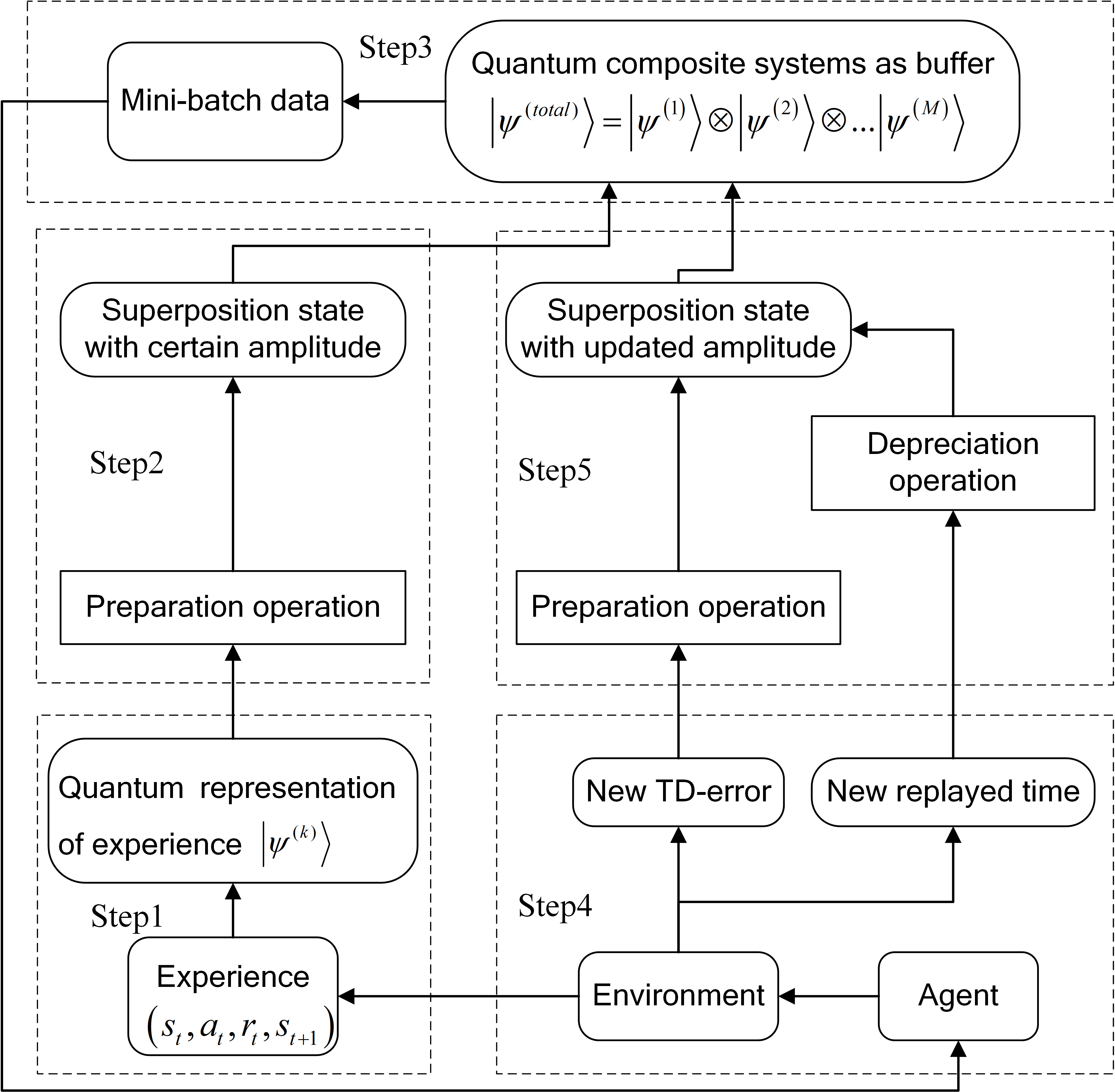
Figure 1: Framework of DRL-QER. Step 1: representing the newly generated experience using a qubit; Step 2: performing the preparation operation on the quantum representation with Grover iteration; Step 3: sampling experiences to compose mini-batch data; Step 4: training the DRL agent with the mini-batch data; Step 5: updating the quantum representation of the experience by the new TD-error (the preparation operation) and the new number of replayed times (the depreciation operation) and then put it back into the replay buffer.

The framework of DRL-QER is described as in Fig. 1. During each learning iteration, the agent interacts with the environment and obtains the transition $e_{t}$ at time step $t$. Such a transition is first expressed in quantum representation, or more precisely, the $k$-th qubit, where $k$ is its index in the buffer. Secondly, the state of the qubit evolves to a superposition state through the preparation operation. Then, transitions are sampled with probabilities proportional to their importance and those selected samples compose the mini-batch data for training the neural network. In addition, after each training step, the amplitudes of the selected quantum representations are manipulated by the combined unitary transformation, including the preparation operation to adapt to the new TD-errors and the depreciation operation to deal with the replaying times of the transitions. This procedure is carried out iteratively until the algorithm converges, whose specific details are implemented in the following subsections.

III-B Quantum Representation of Experiences

In quantum theory, a qubit can be realized by a two-level atom, a spin system or a photon. For two-level atoms, $|0\rangle$ can be the ground state, while $|1\rangle$ represents the excited state. For spin systems, $|0\rangle$ can be the state of spin up, while $|1\rangle$ represents the state of spin down. For photons, $|0\rangle$ can be the state of horizontal polarization, while $|1\rangle$ represents the state of vertical polarization. Here, in experience replay, one experience can be regarded as a qubit system, and its two eigenstates $|0\rangle$ and $|1\rangle$ represent the actions of rejecting and accepting this experience, respectively.

During the learning process, the agent tries to interact with its environment, which can be modeled as an MDP. For each step $t$, with the current state $s_{t}$, the agent selects an action $a_{t}$ under a certain exploration policy (such as $\epsilon$-greedy), and then transfers to the next state $s_{t+1}$, and obtains a reward $r_{t}$. Finally, four elements together compose a transition $(s_{t},a_{t},r_{t},s_{t+1})$, which is assigned a new index $k$ to denote its order in the experience buffer. In transforming the transition into quantum representation, we define the action of accepting and rejecting the transition as two eigenstates. Then, the transition is regarded as a qubit (as shown in Fig. 2) with its state as

$$|\psi^{(k)}\rangle=b_{0}^{(k)}|0\rangle+b_{1}^{(k)}|1\rangle,$$ (7)

where the coefficients $b_{0}^{(k)}$ and $b_{1}^{(k)}$ have probability amplitude meanings, and satisfy $|b_{0}^{(k)}|^{2}+|b_{1}^{(k)}|^{2}=1$. In particular, the probability of rejecting this transition is $|b_{0}^{(k)}|^{2}=|\langle 0|\psi^{(k)}\rangle|^{2}$ and the probability of accepting it is $|b_{1}^{(k)}|^{2}=|\langle 1|\psi^{(k)}\rangle|^{2}$. It is worthy to note that, the coefficients of the qubit are related with the significance of the experience. Before determining its importance, it is practical to first set an initial state, and let the qubit evolve from the initial state to a desired state.

In quantum computing, a uniform state is one significant superposition state, and has the form as

$$|\psi_{0}\rangle=\frac{\sqrt{2}}{2}(|0\rangle+|1\rangle).$$ (8)

It has equal probabilities for two eigenstates and means that least knowledge is given about the state with a maximum entropy, which makes it feasible to adopt the uniform state as the initial state for each experience.

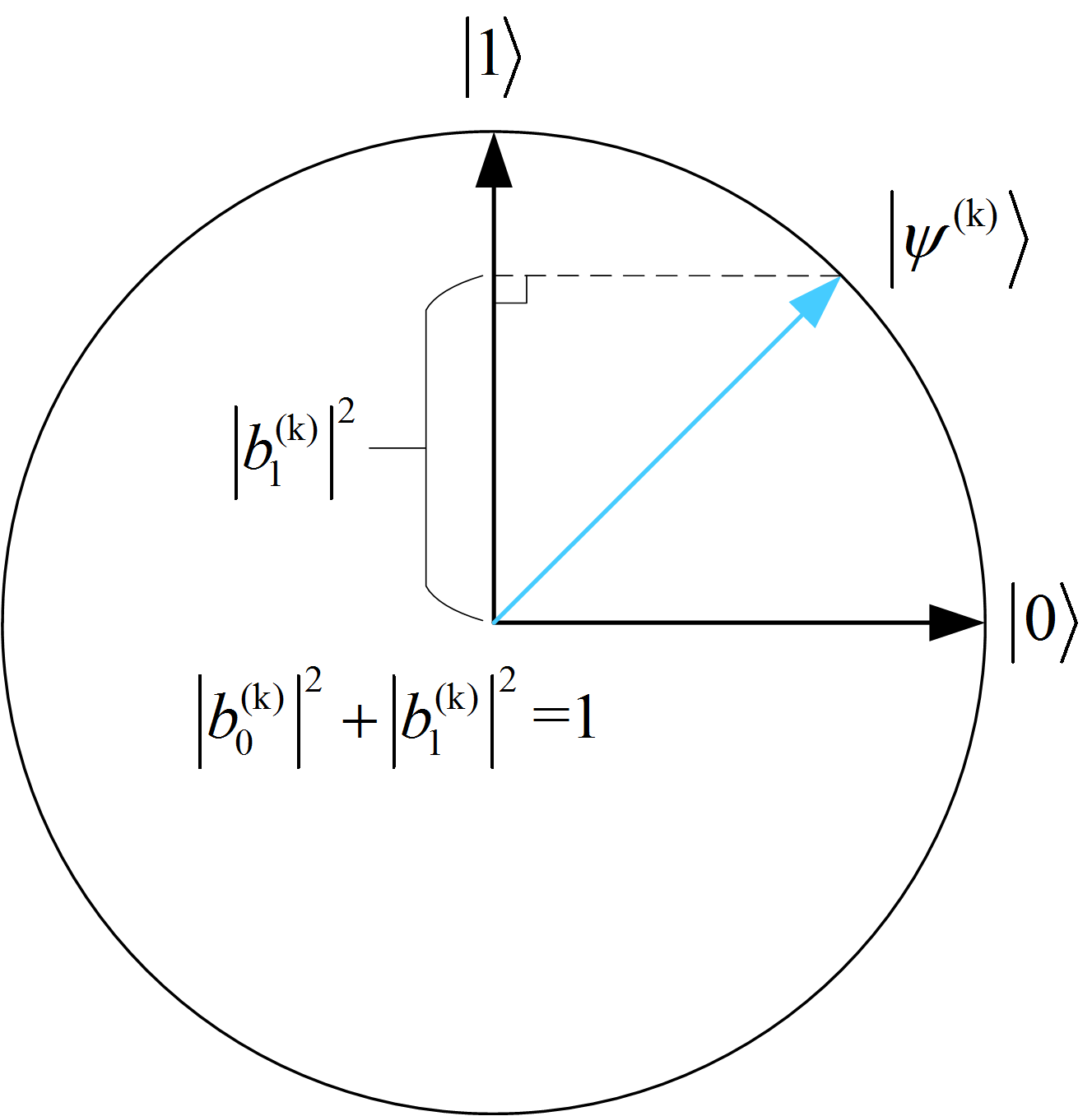
Figure 2: An experience represented in a qubit system. Here, $|0\rangle$ and $|1\rangle$ correspond to rejecting or accepting the transition. The state of such a transition can be formulated as $|\psi\rangle=b_{0}^{(k)}|0\rangle+b_{1}^{(k)}|1\rangle$, where $|b_{1}^{(k)}|^{2}$ is the probability of accepting and $|b_{0}^{(k)}|^{2}$ corresponds to the probability of rejecting.

To adjust the probability amplitudes of the qubit state in (7), a rotation operator, which is the basic element of Grover iteration [20], [31], is applied with

$$U_{\Phi}=e^{-\rm{i}\Phi Y}=\left[\begin{matrix}\textup{cos}(\Phi)&-\textup{sin}(\Phi)\\ \textup{sin}(\Phi)&\textup{cos}(\Phi)\\ \end{matrix}\right],$$ (9)

where $\Phi$ is a real number and has the physical meaning of rotation angle. Pauli $Y$ operator is given as

$$Y\equiv\left[\begin{array}[]{cc}{0}&{-\rm{i}}\\ {\rm{i}}&{0}\end{array}\right].$$ (10)

The operation of performing a rotation operator $U_{\Phi}$ on a qubit of experience is visualized in Fig. 3. The quantum system evolves from the initial state $|\psi_{0}\rangle$ (the green one) to the final state $|\psi_{f}\rangle$ (the blue one), under the unitary transformation $U_{\Phi}$. Projecting $|\psi_{0}\rangle$ and $|\psi_{f}\rangle$ to the $y-$axis, the amplitude of observing $|1\rangle$ increases, which reveals that the probability of accepting the transition is slightly increased.

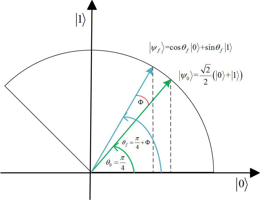
Figure 3: State transition of a qubit system under unitary rotation $U_{\Phi}$, where $|\psi_{0}\rangle$ is the initial state, $|\psi_{f}\rangle$ is the final state.

Since the $k$-th experience in the buffer has the quantum representation form of $\left|\psi^{(k)}\right\rangle$, the state of a memory buffer which is composed of $M$ experiences, is the tensor product of $M$ subsystems:

$$\left|\psi^{\text{ total }}\right\rangle=\left|\psi^{(1)}\right\rangle\otimes\left|\psi^{(2)}\right\rangle\otimes\ldots\left|\psi^{(\mathrm{M})}\right\rangle.$$ (11)

III-C Quantum Operations on Experiences

To deal with the quantum representations of experiences, three sub-processes are involved, i.e., preparation operation, depreciation operation and experience selection by quantum observation. Firstly, the preparation operation is introduced to steer the quantum systems towards the target states, whose amplitudes are related to the TD-errors of the experiences. In fact, whenever the TD-errors of the experiences have changed, the preparation operation is performed to update their probability amplitudes. From this respect, every time when a suitable priority is determined, the quantum systems are to be transferred to a new target state, which can be regarded as a process of quantum state preparation. Hence, we call this special operation as the preparation operation. In addition, the depreciation operation is utilized to make sure that the significance of the experiences is adapted to the experience relaying process, such as the times of the experiences’ being visited. Another significant operation is to select experiences by quantum observation, to compose a mini-batch data for training.

To adjust the amplitudes of quantum systems in a natural and appropriate way, a Grover iteration method is adopted for both the preparation operation and the depreciation operation. Grover iteration is a significant operation for dealing with quantum states originated from classical information, and it aims at intensifying the probabilities of the target eigenstates, with others at equal probabilities [20], [31]. Considering that the probabilities of experiences’ being extracted from an experience buffer vary, we do not use the conventional method, i.e., performing the unitary transformation on the composite system (the whole experience buffer). Instead, Grover iteration is conducted on a single experience with its quantum representation. This strategy helps to adaptively adjust the probability amplitude of each transition, and therefore to circumvent the neglect of the differences between experiences.

III-C1 Preparation operation

To better optimize the process of experience replay in DRL-QER, the importance of experiences needs to be distinguished first. Since a single rotation changes the probability amplitude of a qubit system, we define a basic rotation operator as

$$U_{\sigma}=e^{-\rm{i}\sigma Y}=\left[\begin{array}[]{cc}{\cos(\sigma)}&{-\sin(\sigma)}\\ {\sin(\sigma)}&{\cos(\sigma)}\end{array}\right],$$ (12)

where $\sigma\in R$ is a tiny rotation angle. Based on the exponential approximation formula, i.e., $U_{\Sigma}=(U_{\sigma})^{m}$ with an integer $m$, several iterations of unitary rotations amount to an overall rotation on the qubits. In addition, owing to $e^{-\rm{i}\sigma Y}e^{-\rm{i}(-\sigma)Y}=I$, the rotation in the reverse direction can be conducted with $U_{\sigma}^{-1}$ (or $U_{\sigma}^{\dagger}$). Hence, different rotations can be achieved by performing multiple times of basic rotations in clockwise or counterclockwise directions.

The preparation operation for a single experience (the $k$-th transition in the buffer) is described in Fig. 4, where four times of basic rotations in the counterclockwise direction are performed on the qubit to intensify the “accepting” amplitude of the good experience or equivalently to strength the “rejecting” amplitude of the bad experience. Generally, the state evolution of such a quantum system can be expressed as

$$U_{\Sigma}^{(k)}=(U_{\sigma})^{m_{k}},\quad|\psi_{f}^{(k)}\rangle=U_{\Sigma}^{(k)}|\psi_{0}\rangle,$$ (13)

where $m_{k}$ represents the number of rotation times of the $k$-th qubit. Considering that TD-error reveals the importance of the transition, we associate the value of $m_{k}$ with its TD-error. For transition $e_{t}$ with TD-error $\delta_{t}$, the priority for $k$-th qubit is given as $P_{k}=|\delta_{t}|+\epsilon$ and the maximum priority of all the experiences is $P_{max}$. To convert the priority into the probability amplitude of the qubit, we try to map the priority $P_{k}$ to a rotation angle, which corresponds to a unitary transformation of quantum states. In particular, $P_{max}$ is mapped to a rotation angle $\Sigma_{max}$, and then the angle of $P_{k}$ can be recorded as $\Sigma_{k}=\Sigma_{max}\times\frac{P_{k}}{P_{max}}$. Since Grover iterations aim at iteratively performing unitary transformations until a desired state is achieved, $\Sigma_{max}$ is split into $\mu$ pieces, and each piece is assigned with $\sigma$. The initial state of the qubit is assigned with rotation angle $\iota$, so the angle of rotation can be defined as the target angle minus the initial angle. Finally, the value of $m_{k}$ reads as

$$m_{k}=\textup{Floor}(\mu\times P_{k}/P_{max}-\iota/\sigma),$$ (14)

where $\mu,\iota\in R$ are two hyper-parameters, and $\textup{Floor}(x)$ takes the largest integer not greater than $x$. In particular, the sign of $m_{k}$ reflects the rotation direction relative to the angle of the uniform state, i.e., $\frac{\pi}{4}$. For example, when $m_{k}$ is a positive integer, Grover iteration works in the counterclockwise direction, otherwise, it is conducted in the clockwise direction.

The value of $\sigma$ in (13) is usually carefully set since it plays an important role in the quantum representation of experiences. From a convenient point of view, it is the most appropriate to set a fixed value. While from the perspective of adaptation to different environments, associating it with the training process, such as the TD-errors, the maximum times of experiences’ being visited and the training steps is more preferable. In this work, we describe it with a function associated with the training episode $TE$:

$$\sigma=\frac{\zeta_{1}}{1+e^{\frac{TE}{\zeta_{2}}}},$$ (15)

where $\zeta_{1},\zeta_{2}\in R$ are two hyper-parameters.

By performing the same procedure to each transition, all experiences will end up in their target quantum representations. For example, for most of those valuable transitions, performing the preparation operation in the counterclockwise direction makes them approach $|1\rangle$, while for those less important experiences, the preparation operation in clockwise direction can be deployed on their quantum representations to make them closer to $|0\rangle$.

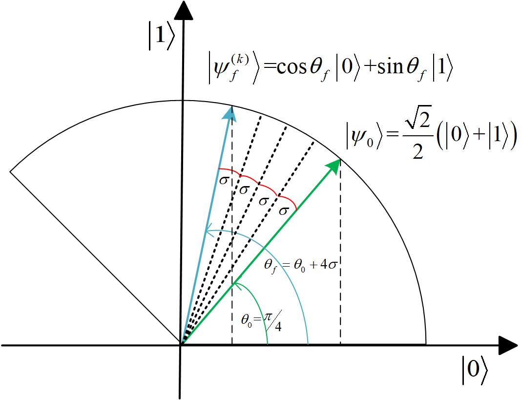
Figure 4: The procedure of the preparation process using Grover iterations for the $k$-th qubit. $|\psi_{0}\rangle$ is the uniform quantum state, $|\psi_{f}^{(k)}\rangle$ is the quantum state after conducting the transformation $U_{\Sigma}^{(k)}$.

III-C2 Depreciation operation

After the process of preparation, the probabilities of selecting the experiences are closely associated with their TD-errors. However, in actual training, some experiences are replayed at high frequencies and may result in poor learning performance, which is called over-training, and the limited size of the replay buffer may aggravate this situation [43]. In RL, over-training reveals the issue of exploration–exploitation tradeoff [44, 45, 46, 47, 48, 49]. Sufficient exploration in the state-action space helps prevent the algorithm being trapped in locally optimal solutions, while exploiting the current policy helps the algorithm converge as fast as possible. To achieve a balance between exploration and exploitation, the sample diversity is considered to enhance the learning performance of the agent. As such, the depreciation operation is developed for the experiences according to the replaying process. This is achieved by iteratively modifying their probabilities once the transitions are selected, whose effect contains and is greater than the utilization of importance-sampling correction, which is demonstrated in the ablation experiments in the supplementary material.

Once the experiences are selected and put back in the memory buffer for training, their importance to the agent is unavoidably changed, not only because their TD-errors have been changed, but also in that they are no longer brand new to the agent. Therefore their probability amplitudes need to be modified. From this perspective, another unitary transformation

$$U_{\omega}=\left[\begin{array}[]{cc}{\cos(\omega)}&{-\sin(\omega)}\\ {\sin(\omega)}&{\cos(\omega)}\end{array}\right]$$ (16)

is used for the depreciation operation, with $\omega\in R$. In particular, it is implemented on the selected experiences using Grover iteration. Every time the experiences have been accepted, their quantum representations go through a unitary transformation as follows

$$|\psi^{(k)}_{f}\rangle\leftarrow U_{\omega}|\psi^{(k)}_{f}\rangle.$$ (17)

The value of $U_{\omega}$, or more precisely $\omega$, should be adapted to the specific scenario. In experience replay, when the buffer is full, new transitions are orderly put in the buffer, with the old ones replaced. Besides, the period of the experiences’ being replaced is a fixed number of steps. Hence, a transition will be kept in the buffer for fixed time steps, before it is replaced. In that case, during fixed training steps, the total replaying times of all the experiences are fixed. A large value of the maximum number of replaying times among all the experiences (denoted as $RT_{\max}$) reveals an uneven replaying distribution, which means that some experiences have outstanding priorities compared to other experiences. To weaken this phenomena, a smaller $\omega$ helps to retain those less important experiences; otherwise, a large depreciation factor might result in sharp declines in the accepting probabilities of those experiences. Hence, the value of $\omega$ is decreased with $RT_{\max}$.

In addition, $\omega$ should be adapted to the training episode $TE$. In the early training stage, the importance of experiences is ambiguous. While, after a period of training, the TD-errors of some experiences tend to remain in large values, no matter how many times they have been selected to update the network. Therefore, it is feasible to “intensify” the accepting probabilities of the experiences that have been replayed with more times compared with others at the early training stage and to “cool” down their accepting probabilities to avoid over-training at the later stage. This is realized by increasing $\omega$ with the training episode $TE$. Finally, the depreciation factor $\omega$ is given as

$$\omega=\frac{\tau_{1}}{RT_{\max}(1+e^{\tau_{2}/TE})},$$ (18)

where $\tau_{1},\tau_{2}\in R$ are two hyper-parameters.

III-C3 Experience selection by quantum observation

To accomplish the training process, samples are chosen from the buffer and fed into the network for learning. Here, we draw from the quantum measurement principle and determine the probabilities of experiences based on quantum observation. For the $k$-th qubit in state $|\psi^{(k)}_{f}\rangle$, observing its probability of being accepted is $|\langle 1|\psi^{(k)}_{f}\rangle|^{2}$, which is actually the probability of measuring $|1\rangle$. Then, normalizing the probability based on all transitions, we obtain its replaying probability as

$$b_{k}=\frac{|\langle 1|\psi^{(k)}_{f}\rangle|^{2}}{\sum_{i}|\langle 1|\psi^{(i)}_{f}\rangle|^{2}}.$$ (19)

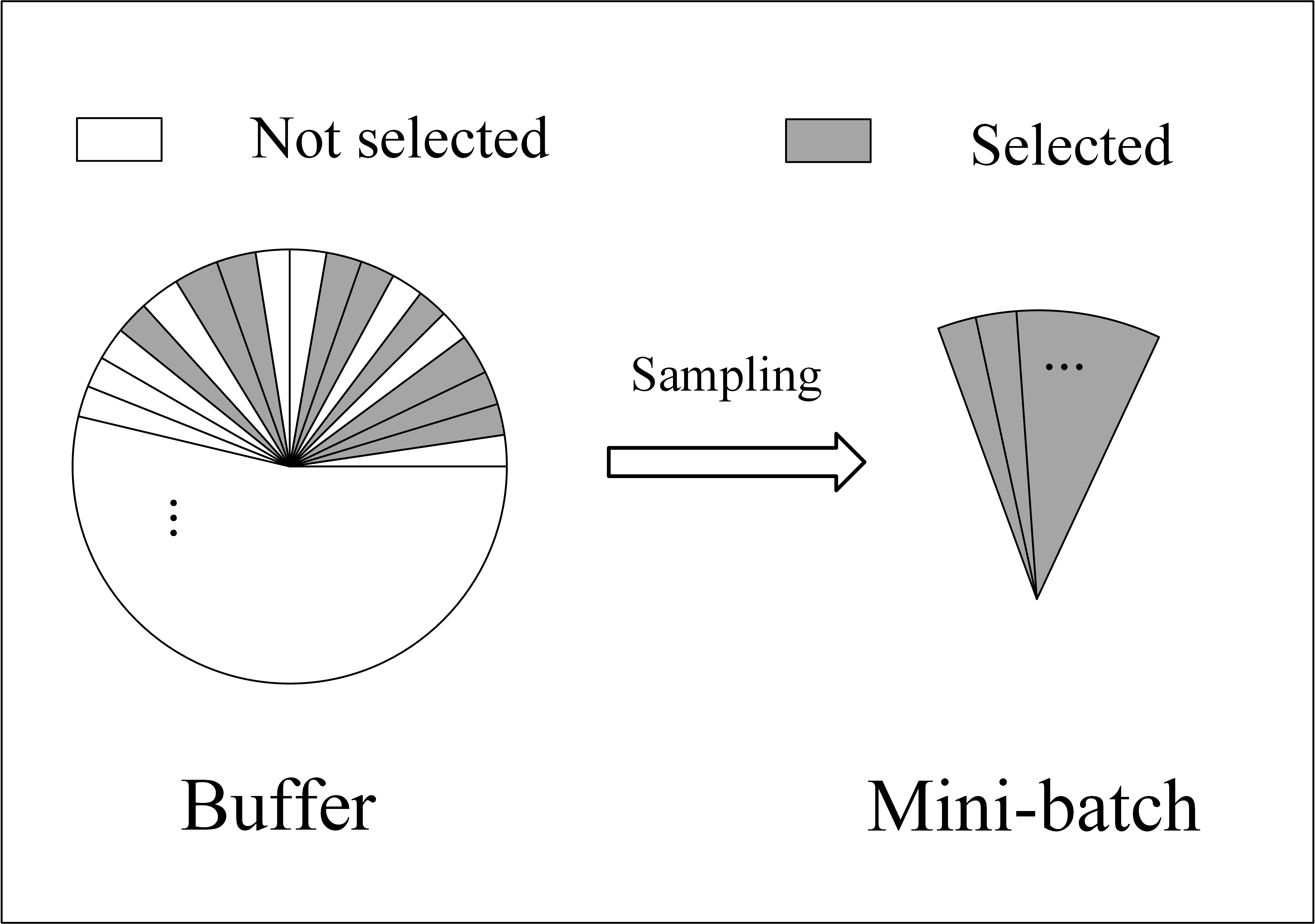
Figure 5: The observation process for experience replay. The buffer is composed of a number of transitions, where each one is accompanied with its probability drawn from quantum observation principle. The transitions are sampled out from buffer according to their replaying probabilities to compose the mini-batch data.

The process of experience selection is summarized as in Fig. 5, where each transition has its own probability in the buffer. Inspired by the quantum observation principle, this process determines the probabilities of being selected among the buffer. During the sampling process, several times of sampling one transition from the experience buffer are performed under fixed probabilities. The sampling times are consistent with the size of minibatch, which is set as $32$ in the simulations.

Remark 1.

The process of obtaining minibatch data from the buffer with fixed probabilities is a sampling process with replacement. For each sampling process, the selected sample is still retained in the buffer and is reset to the uniform state after being sampled. This idea is inspired from the phenomena that observing a quantum system makes its state collapses. In that case, the quantum operation (i.e., the preparation operation and the depreciation operation) on the selected quantum experience starts from the uniform state, rather than its previous state.

III-D Implementation

Input: size of experience buffer $M$, size of mini batch $N$.

Initialize the preparation factor $\sigma$, the depreciation factor $\omega$, the maximum TD-error $\delta_{\max}$, the replayed time vector $cn=[cn_{1},cn_{2},\ldots,cn_{M}]=\vec{0}$, the index in the buffer $k=1$, a variable $LF=False$;

for $TE=1\to TrainingFrames$ do

       Observe $s_{1}$ and choose $a_{1}\sim\pi(s_{1})$;

       for $t=1\to T$ do

             Observe $r_{t},s_{t+1}$ and then obtain a transition $e_{t}$;

             if $s_{t+1}$ is terminal then

                  break;

             end if

            

            Initialize the $k$-th qubit as the uniform state $|\psi_{0}\rangle$;

             Set $P_{k}=|\delta_{max}|$ and obtain $m_{k}$ according to (14);

             Perform the preparation operation on $k$-th qubit using Grover iteration, and obtain its final state $|\psi^{(k)}_{f}\rangle=(U_{\sigma})^{m_{k}}|\psi_{0}\rangle$;

            

            Store the transition $e_{t}$ with its quantum representation $|\psi^{(k)}_{f}\rangle$ in the buffer;

            

            if LF==True then

                  Determine the probabilities of the experiences by quantum observations and obtain their replaying probabilities $\left[b_{1},b_{2},...,b_{M}\right]$ according to (19);

                   Update the preparation factor $\sigma$ and the depreciation factor $\omega$;

                   for $j=1\to N$ do

                         Sampling a transition with its index in the buffer as $d\in\{1,2,...,M\}$ based on $\left[b_{1},b_{2},...,b_{M}\right]$;

                         Reset the $d$-th qubit back to the uniform state $|\psi_{0}\rangle$;

                         Compute its TD-error $\delta_{j}=r_{j}+\eta\max_{a}Q_{target}(s_{j+1},a)-Q(s_{j},a_{j})$;

                         Obtain its priority $P_{d}=|\delta_{j}|$ and obtain $m_{d}$ according to (14);

                         Update the replaying time $cn_{d}$ by $cn_{d}=cn_{d}+1$;

                        

                        Conduct a complex Grover iteration process including both the preparation operation and the depreciation operation on the experience’s quantum representation $|\psi^{(d)}_{f}\rangle=(U_{\omega})^{cn_{d}}(U_{\sigma})^{m_{d}}|\psi_{0}\rangle$;

                         Update $\delta_{max}=\max(\delta_{max},|\delta_{j}|)$ and update $RT_{\max}=\max(cn_{1},cn_{2},...,cn_{M})$;

                        

                   end for

                  

                  Update weights $\theta$ by stochastic gradient descent;

                   Copy weights into target network $\theta_{target}\leftarrow\theta$;

                   Remove the $k$-th quantum representation of experience from the buffer and reset $cn_{k}=0$;

                  

             end if

            

            $k\leftarrow k+1$;

             if $k>M$ then

                   Set $LF=True$ and set $k=1$;

             end if

            

            Choose action $a_{t+1}\sim\pi(s_{t+1})$;

            

       end for

      

end for

Algorithm 1 DRL-QER Algorithm

An integrated DRL-QER algorithm is shown as in Algorithm 1. During each step, the agent encounters transition $e_{t}$. Considering that the newly generated transition does not have a TD-error, we assign the maximum TD-error for it, i.e., $\delta_{t}=\delta_{\max}$ to give it a high priority. This guarantees that every new experience is sampled with a high priority. Then, the transition is represented as a qubit, with its initial state as $|\psi_{0}\rangle$. The preparation operation using Grover iteration is performed on the experience until it reaches the final state $|\psi^{(k)}_{f}\rangle$. After the buffer is full, transitions are sampled with probabilities proportional to their amplitudes of quantum states, and those selected samples compose the mini-batch data for training the network. For the selected transitions, after being reset to the uniform state, their corresponding quantum representations are manipulated through the preparation operation to adapt to new priorities, and the depreciation operation to adapt to the replaying times. This procedure is carried out iteratively until the algorithm converges.

Remark 2.

The proposed QRL-QER method works by representing the classical information (experiences) into quantum forms and performing quantum operations. Although it is inspired by quantum laws, the process can be simulated on a classical device. Hence, it is a quantum-inspired algorithm, and does not need to be implemented on a quantum device.

Remark 3.

In DRL, the buffer is to store the past experiences and use them to update the parameters of the agent. During this process, the agent interacts with the environment under the new network parameters. Hence, the experiences in the buffer should be updated after some training steps to gain a better training effect. To achieve this, the buffer is set as a fixed size and the oldest experience is discarded to make room for the newly produced experience (reset $k=1$ in Algorithm 1) when the buffer is full ($k>=M$ in Algorithm 1). In addition, the procedure of updating the parameters of the network begins after the buffer is full, i.e., the variable $LF$ is set $True$. This technique is also applied to DRL-PER and DCRL to achieve a fair comparison in the following experiment section. In the implementation of Algorithm 1, we set a predefined value for the maximum value of TD-error, i.e., $\delta_{\max}$. During the whole learning process, $\delta_{\max}$ should be updated once a larger TD-error is found. As such, new $\delta_{\max}$ is assigned to the future newly generated transitions to give them the highest priorities.

IV Experiments

To test the proposed DRL-QER algorithm, several groups of experiments are carried out on Atari games with comparison to two benchmark algorithms (DRL-PER and DCRL). In addition, DRL-QER is combined with double network and dueling network, and tested on additional experiments to verify its performance.

IV-A Setup

The experiments are carried out on the widely used platform OpenAI Gym to play Atari 2600 games [50], and the testing games can be divided into four categories, namely shooting games, antagonistic games, racing games and strategy games. For all the games, the agent takes high-dimensional data ($210\times 160$ colour video) as input to learn good policies. In order to win the games, the agent has to plan over the long-term. All the experiments are deployed on a computer of ThinkStation P920 with 24xCPU@2.40GHz, Nvidia Tesla p5000, Ubuntu 16.04.5 LTS, Python.

To verify the effectiveness of DRL-QER, two baseline algorithms including DRL-PER [13] and DCRL [14] are also tested for comparison. The sampling method in DRL-QER can be regarded as a generalization of that in DRL-PER. DRL-PER samples experiences according to their TD-errors with proportional prioritization, and this can be regarded as a situation in which DRL-QER does not consider the influence of over-training and discards the depreciation operation.

When deploying DRL-QER on Atari 2600 games, we adopt a similar neural network architecture and a same hyper-parameter setting to those in [11] and [13]. Considering the hardware limitation, the high computational requirement and the high time cost, we make some fine-tuning on the hyper-parameters. In order to avoid the expensive cost of training for 50 million frames, we train for 5 million frames. Generally, it is hard and not necessary to accomplish quantum operations on a classical computer. We need to do necessary approximation in the simulation of DRL-QER, i.e., the states of qubit systems are represented by two-dimensional complex vectors, and the preparation operation and the depreciation operation are performed in the form of unitary matrix transformation. In addition, the normalized probabilities are stored in a special binary heap called “sum tree”, where the value of a parent node is the sum of all values of its children. Last but not least, for performing necessary operations on experiences, we introduce some hyper-parameters for the preparation factor $\sigma$ and the depreciation factor $\omega$, and their values are provided in Table I. Other hyper-parameters of DRL-QER are selected by performing a grid search on the game Breakout.

TABLE I: Hyper-parameters Adjustments in Numerical Experiments

Altered Hyper-parameters
Hyper-parameter	Original Value	Altered Value
Training Frames	$5\times 10^{7}$	$5\times 10^{6}$
Preparation sub-factor $\zeta_{1}$	—	$0.03\pi$
Preparation sub-factor $\zeta_{2}$	—	$2\times 10^{6}$
Depreciation sub-factor $\tau_{1}$	—	$\pi$
Depreciation sub-factor $\tau_{2}$	—	$1\times 10^{6}$
Parameter $\mu$ of $m$	—	100
Parameter $\iota$ of $m$	—	$0.25\pi$

TABLE II: Average Rewards Per Episode of DRL-PER, DCRL and DRL-QER

Game Name	DRL-PER($\pm$std)	DCRL($\pm$std)	DRL-QER($\pm$std)
Alien	1270.2($\pm 341.3$)	1223.9($\pm 297.1$)	1309.3($\pm 348.8$)
Beam Rider	1448.3($\pm 290.2$)	1594.6($\pm 302.3$)	1508.2($\pm 330.4$)
Breakout	5.7($\pm 2.1$)	5.2($\pm 1.9$)	5.8($\pm 2.8$)
Carnival	1142.5($\pm 376.2$)	1235.1($\pm 331.5$)	1214.0($\pm 413.4$)
Enduro	43.0($\pm 20.6$)	44.3($\pm 20.5$)	42.7($\pm 19.2$)
Freeway	60.6($\pm 6.6$)	60.2($\pm 5.8$)	60.7($\pm 6.3$)
Kangaroo	1129.3($\pm 291.3$)	1237.3($\pm 303.2$)	1143.3($\pm 324.6$)
Kung-Fu Master	521.3($\pm 328.8$)	670.0($\pm 434.8$)	712.0($\pm 370.9$)
Ms. Pacman	1862.2($\pm 661.8$)	1918.9($\pm 741.2$)	1903.5($\pm 735.3$)
River Raid	2248.6($\pm 626.8$)	1239.5($\pm 251.6$)	1479.5($\pm 307.5$)
Road Runner	2312.7($\pm 897.7$)	3615.3($\pm 1543.8$)	3208.7($\pm 1298.7$)
Space Invaders	679.2($\pm 321.2$)	735.1($\pm 250.8$)	741.5($\pm 317.2$)

TABLE III: Average Rewards Per Episode of DRL-PER with double network and DRL-QER with double network

Game Name	DRL-PER($\pm$std)	DRL-QER($\pm$std)
Alien	1215.2($\pm 392.0$)	1275.0($\pm 350.0$)
Carnival	2420.5($\pm 315.2$)	2480.3($\pm 319.2$)
River Raid	1906.2($\pm 522.6$)	1870.9($\pm 310.7$)
Space Invaders	723.6($\pm 229.9$)	750.3($\pm 262.8$)

TABLE IV: Average Rewards Per Episode of DRL-PER with dueling network and DRL-QER with dueling network

Game Name	DRL-PER($\pm$std)	DRL-QER($\pm$std)
Alien	801.4($\pm 131.6$)	854.6($\pm 140.3$)
Carnival	1317.0($\pm 376.5$)	1367.7($\pm 380.2$)
River Raid	3249.2($\pm 522.0$)	3007.3($\pm 456.7$)
Space Invaders	756.1($\pm 229.5$)	758.8($\pm 262.2$)

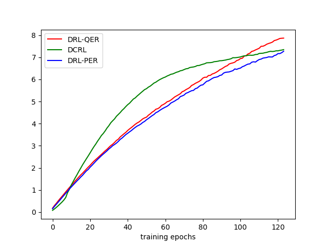
(a) Space Invaders

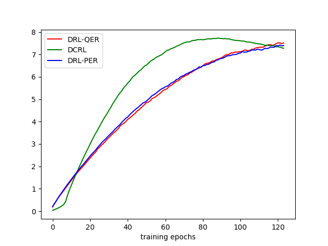
(b) Carnival

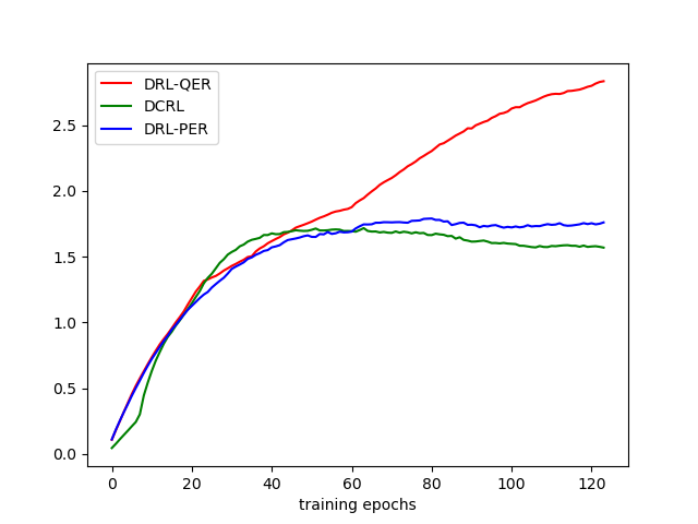
(c) Breakout

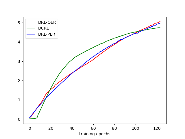
(d) Freeway

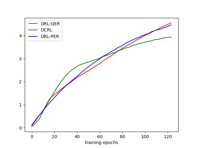
(e) Beam Rider

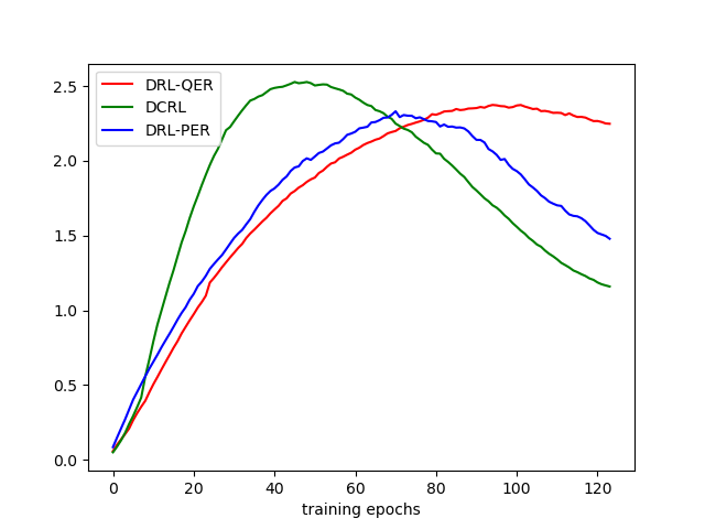
(f) Kung-Fu Master

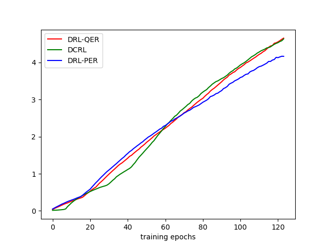
(g) Road Runner

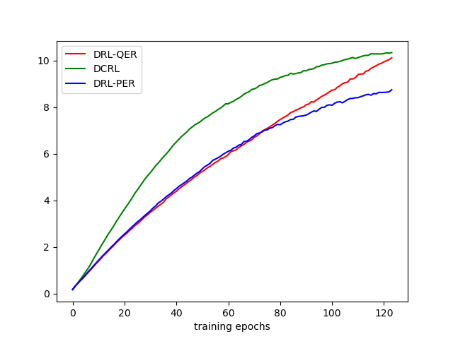
(h) River Raid

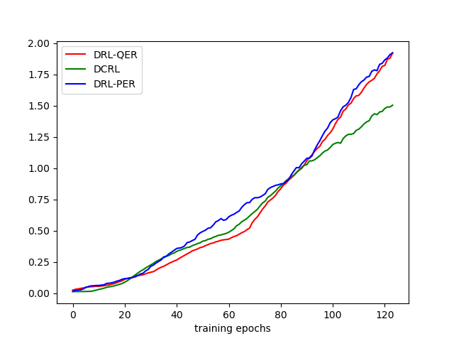
(i) Enduro

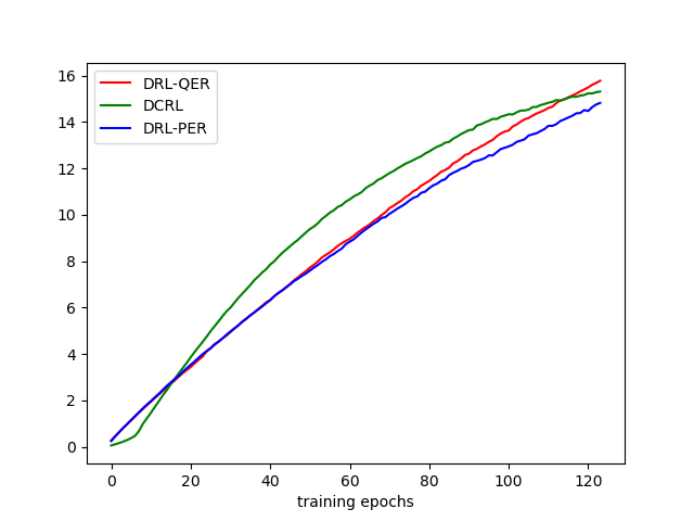
(j) Ms. Pacman

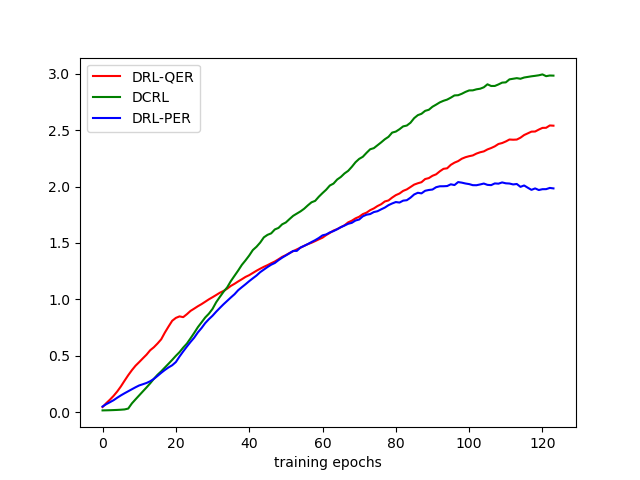
(k) Kangaroo

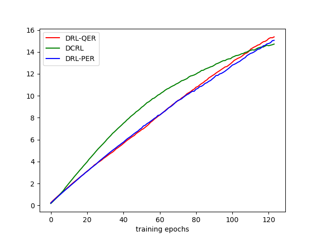
(l) Alien

Figure 6: Performance of DRL-QER with comparison to DRL-PER and DCRL regarding the average Q value.

IV-B Experimental Results

The experiments of the twelve games are deployed to compare the performance of DRL-PER, DCRL and DRL-QER. Similar to DCRL [14], AER [16] and CER [17], each simulation is run for three times to collect the average performance for a fair comparison. After the training process, we test the agents for 150 episodes, and the average rewards with the standard deviation are summarized in Table II. It is clear that DRL-QER outperforms DRL-PER in most of the testing games. The statistical analysis also reveals that DRL-QER and DCRL achieve a comparative performance for the twelve games and they have different advantages in different games. Considering the total reward metric tends to be noisy because small changes to the weights of the DRL agent can lead to large changes in the distribution of states the agent visits [11], we take the estimated action-value as the metric, which has been demonstrated to be more stable than reward metric to reveal the training performance of DRL methods. In particular, we divide the training phase into 125 epochs, and the average action values of the testing frames are recorded after each training epoch. The experimental results demonstrate that the learning progress of DRL-QER is faster and more robust than that of DRL-PER, and is not worse than DCRL. It is worthy to note that DRL-QER merely changes the priorities of experiences without affecting the convergence of the baseline DRL method [13]. However, an efficient use of samples contributes to a faster convergence under limited training epochs. Hence, the trends of the training curves (shown in Fig. 6) reflect the superiority of our method. What’s more, DCRL involves many parameters which are difficult to fine tune for different games, while DRL-QER does not require prior knowledge to fine tune parameters. In fact, the parameter settings of DRL-QER are almost the same across the twelve games. From this respective, DRL-QER is an effective and general approach with enhanced performance.

IV-C Additional Exploratory Experiments

The proposed DRL-QER aims at taking advantage of quantum characteristics in the experience replay mechanism. To figure out whether this mechanism can be applied to other memory-based RL algorithms, we further apply DRL-QER to double network [51] and dueling network [52], and implement experimental simulations on randomly selected 4 games using the same hyper-parameter setting in Table I. In Fig. 7, both double DQN and dueling DQN algorithms using the quantum-inspired experience replay (QER) method show faster convergence regarding the average Q value compared with their classical counterparts. The average rewards of DRL-QER-Double and DRL-PER-Double are summarized in Table III. Besides, the average rewards of DRL-QER-Dueling and DRL-PER-Dueling are summarized in Table IV. From these two tables, the average rewards per episode are also increased in ”Double Network” and ”Dueling Network” for 3 games except for Riverraid.

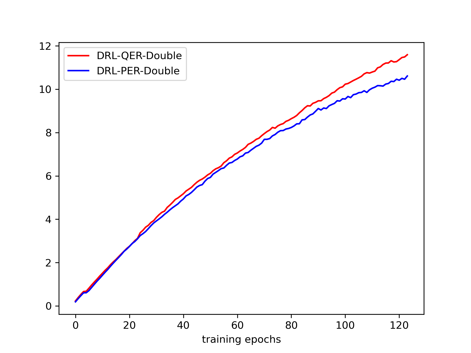
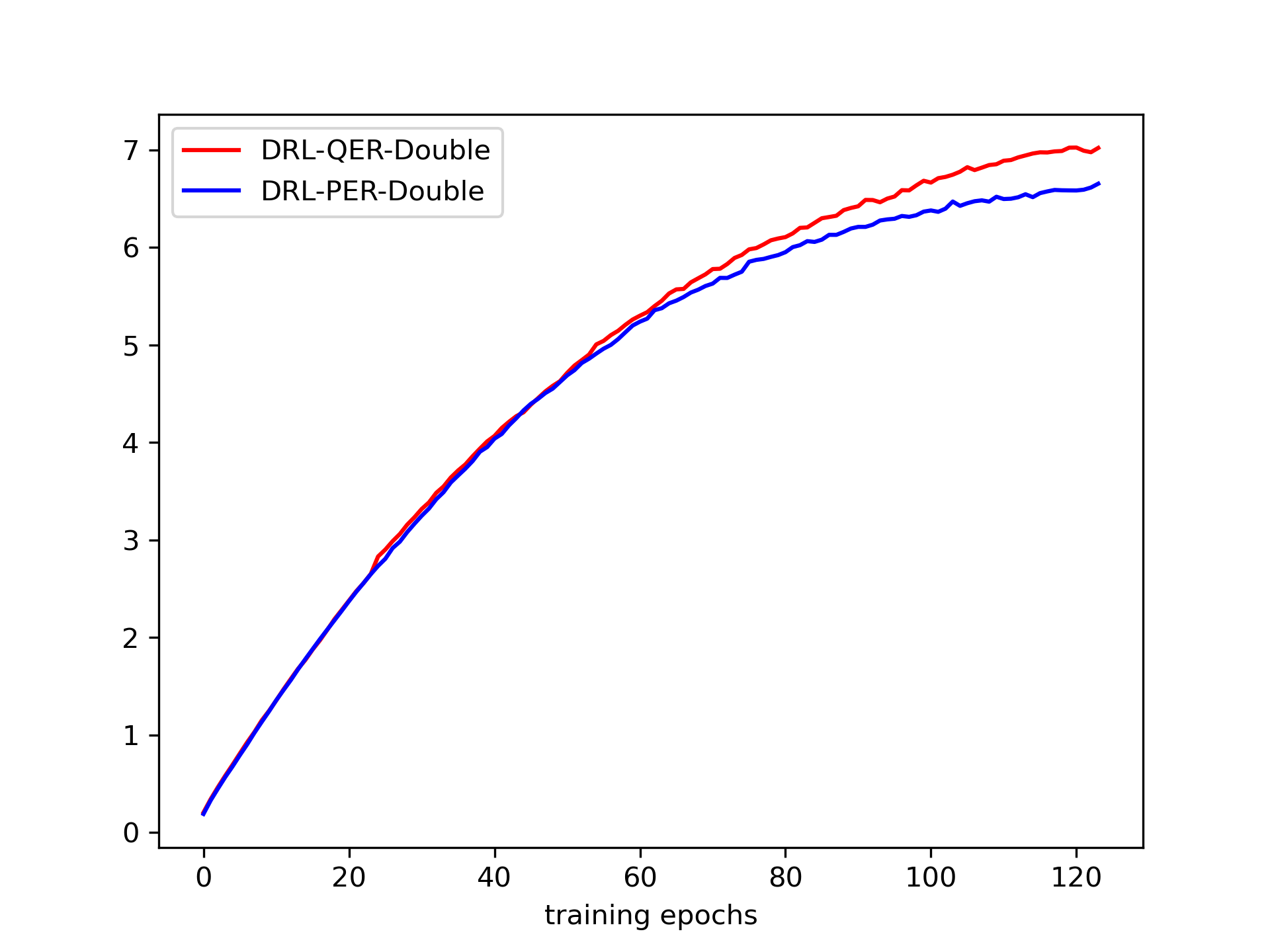
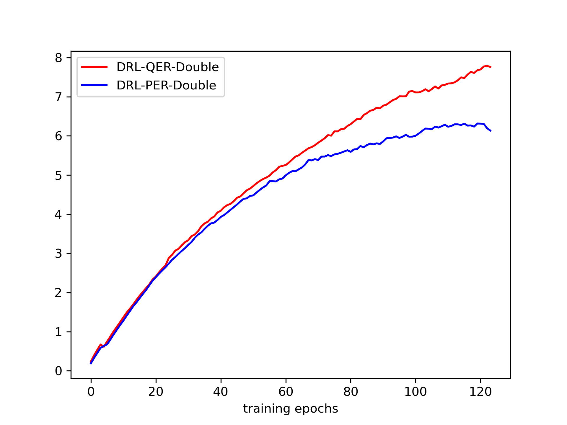
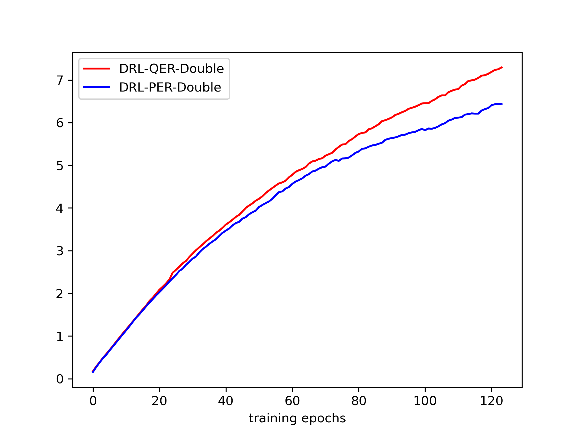
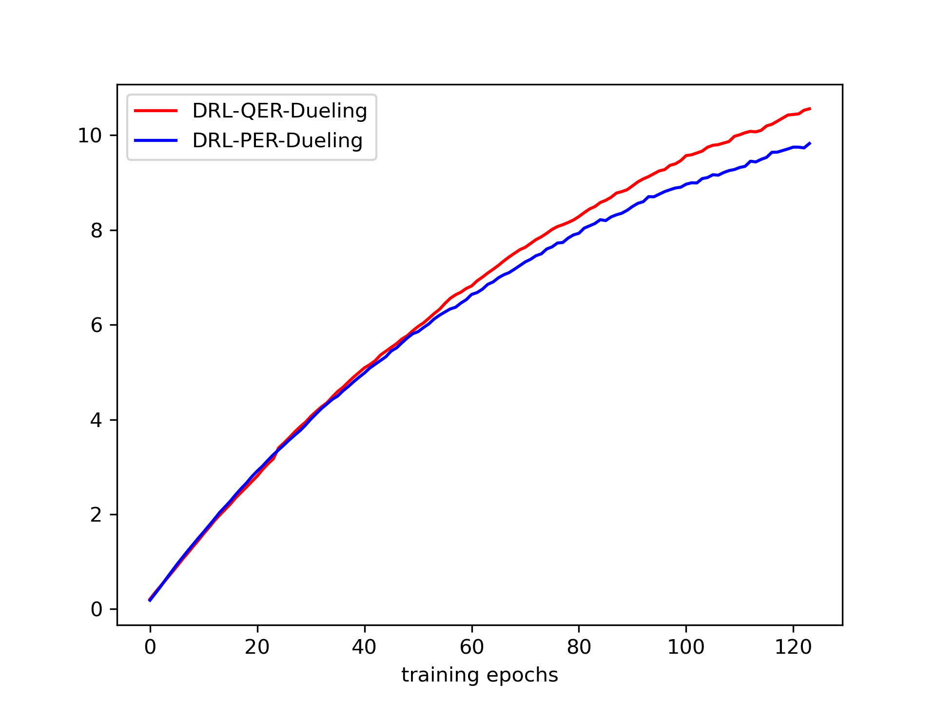
(a) Alien

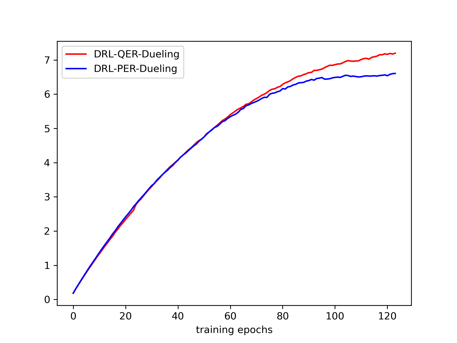
(b) Carnival

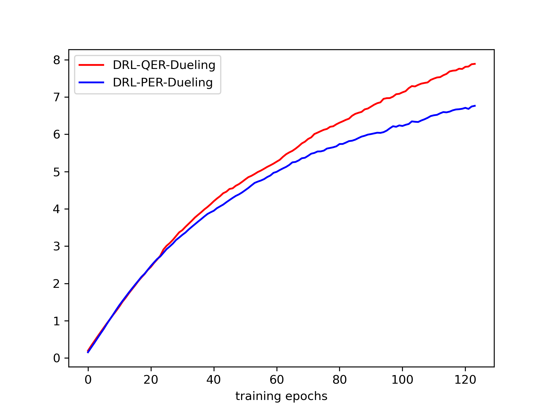
(c) River Raid

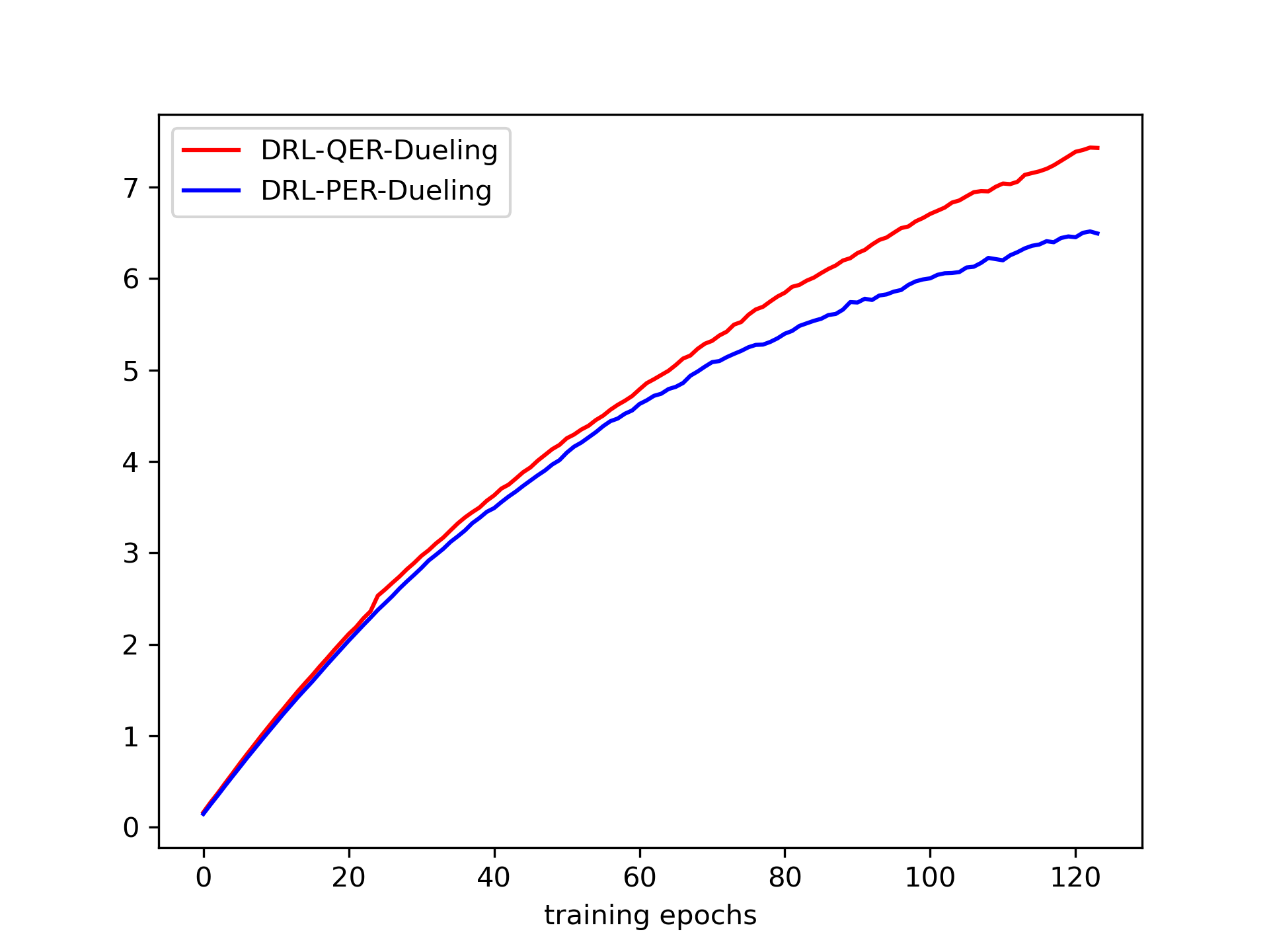
(d) Space Invaders

Figure 7: Performance of DRL-QER-Double/DRL-PER-Double and DRL-QER-Dueling/DRL-PER-Dueling regarding the average Q value.

V Conclusion

In this paper, the DRL-QER method is proposed by introducing quantum characteristics into the process of experience replay in DRL to guarantee that the learning scheme focuses on what the agent has learnt from the interaction with the environment instead of the prior knowledge. In DRL-QER, the experiences are represented in quantum states, whose amplitudes are correlated with the TD-errors and the replaying times. In particular, the preparation operation and the depreciation operation in DRL-QER help speed up the training progress and achieve an improved sampling efficiency. The experimental results demonstrate superior performance of the proposed DRL-QER over DRL-PER and DCRL. Comparisons of DRL-PER and DRL-QER in dueling DQN and double DQN further show that DRL-QER can also achieve improved performance for other memory-based DRL algorithms. Our future work will focus on in-depth theoretical research on the convergence of DRL-QER and quantum enhanced reinforcement learning along with its applications to other continuous control methods such as deep deterministic policy gradient (DDPG) [53], [54] and Soft Actor Critic [55].

References

- [1] R. S. Sutton and A. G. Barto, Reinforcement learning: An introduction (2nd Edition). MIT Press, 2018.
- [2] M. L. Littman, “Reinforcement learning improves behaviour from evaluative feedback,” Nature, vol. 521, pp. 445–451, May 2015.
- [3] J.-A. Li, D. Dong, Z. Wei, Y. Liu, Y. Pan, F. Nori, and X. Zhang, “Quantum reinforcement learning during human decision-making,” Nature Human Behaviour, vol. 4, pp. 294–307, March 2020.
- [4] A. Krizhevsky, I. Sutskever, and G. E. Hinton, “Imagenet classification with deep convolutional neural networks,” in Advances in Neural Information Processing Systems, pp. 1097–1105, 2012.
- [5] C. Farabet, C. Couprie, L. Najman, and Y. LeCun, “Learning hierarchical features for scene labeling,” IEEE Transactions on Pattern Analysis and Machine Intelligence, vol. 35, pp. 1915–1929, August 2013.
- [6] H. Goh, N. Thome, M. Cord, and J.-H. Lim, “Learning deep hierarchical visual feature coding,” IEEE Transactions on Neural Networks and Learning Systems, vol. 25, pp. 2212–2225, December 2014.
- [7] H. Geoffrey, D. Li, Y. Dong, E. D. George, and A.-r. Mohamed, “Deep neural networks for acoustic modeling in speech recognition: The shared views of four research groups,” IEEE Signal Processing Magazine, vol. 29, pp. 82–97, November 2012.
- [8] I. Sutskever, O. Vinyals, and Q. V. Le, “Sequence to sequence learning with neural networks,” in Advances in Neural Information Processing Systems, pp. 3104–3112, 2014.
- [9] P. P. Brahma, D. Wu, and Y. She, “Why deep learning works: A manifold disentanglement perspective,” IEEE Transactions on Neural Networks and Learning Systems, vol. 27, pp. 1997–2008, October 2015.
- [10] H. Tembine, “Deep learning meets game theory: Bregman-based algorithms for interactive deep generative adversarial networks,” IEEE Transactions on Cybernetics, vol. 50, pp. 1132–1145, March 2020.
- [11] V. Mnih, K. Kavukcuoglu, D. Silver, A. A. Rusu, J. Veness, M. G. Bellemare, A. Graves, M. Riedmiller, A. K. Fidjeland, G. Ostrovski, et al., “Human-level control through deep reinforcement learning,” Nature, vol. 518, p. 529, February 2015.
- [12] L.-J. Lin, “Self-improving reactive agents based on reinforcement learning, planning and teaching,” Machine Learning, vol. 8, no. 3-4, pp. 293–321, 1992.
- [13] T. Schaul, J. Quan, I. Antonoglou, and D. Silver, “Prioritized experience replay,” in Proceedings of the IEEE International Conference on Learning Representations, 2016.
- [14] Z. Ren, D. Dong, H. Li, and C. Chen, “Self-paced prioritized curriculum learning with coverage penalty in deep reinforcement learning,” IEEE Transactions on Neural Networks and Learning Systems, vol. 29, pp. 2216–2226, June 2018.
- [15] G. Novati and P. Koumoutsakos, “Remember and forget for experience replay,” in Proceedings of the 36th International Conference on Machine Learning (K. Chaudhuri and R. Salakhutdinov, eds.), vol. 97 of Proceedings of Machine Learning Research, (Long Beach, California, USA), pp. 4851–4860, PMLR, 09–15 Jun 2019.
- [16] P. Sun, W. Zhou, and H. Li, “Attentive experience replay,” in The Thirty-Fourth AAAI Conference on Artificial Intelligence, AAAI 2020, The Thirty-Second Innovative Applications of Artificial Intelligence Conference, IAAI 2020, The Tenth AAAI Symposium on Educational Advances in Artificial Intelligence, EAAI 2020, New York, NY, USA, February 7-12, 2020, pp. 5900–5907, AAAI Press, 2020.
- [17] H. Liu, A. Trott, R. Socher, and C. Xiong, “Competitive experience replay,” in 7th International Conference on Learning Representations, ICLR 2019, New Orleans, LA, USA, May 6-9, 2019, OpenReview.net, 2019.
- [18] H.-S. Chang, E. Learned-Miller, and A. McCallum, “Active bias: Training more accurate neural networks by emphasizing high variance samples,” in Advances in Neural Information Processing Systems, pp. 1002–1012, 2017.
- [19] P. W. Shor, “Algorithms for quantum computation: Discrete logarithms and factoring,” in Proceedings 35th Annual Symposium on Foundations of Computer Science, pp. 124–134, 1994.
- [20] L. K. Grover, “Quantum computers can search arbitrarily large databases by a single query,” Physical Review Letters, vol. 79, pp. 4709–4712, December 1997.
- [21] J. Biamonte, P. Wittek, N. Pancotti, P. Rebentrost, N. Wiebe, and S. Lloyd, “Quantum machine learning,” Nature, vol. 549, pp. 195–202, September 2017.
- [22] X.-D. Cai, D. Wu, Z.-E. Su, M.-C. Chen, X.-L. Wang, L. Li, N.-L. Liu, C.-Y. Lu, and J.-W. Pan, “Entanglement-based machine learning on a quantum computer,” Physical Review Letters, vol. 114, p. 110504, March 2015.
- [23] Z. Li, X. Liu, N. Xu, and J. Du, “Experimental realization of a quantum support vector machine,” Physical Review Letters, vol. 114, p. 140504, April 2015.
- [24] K. Beer, D. Bondarenko, T. Farrelly, T. J. Osborne, R. Salzmann, D. Scheiermann, and R. Wolf, “Training deep quantum neural networks,” Nature Communications, vol. 11, p. 808, 2020.
- [25] L. Bai, L. Rossi, L. Cui, J. Cheng, and E. R. Hancock, “A quantum-inspired similarity measure for the analysis of complete weighted graphs,” IEEE Transactions on Cybernetics, vol. 50, pp. 1264–1277, March 2020.
- [26] W. Ding, C. Lin, and Z. Cao, “Deep neuro-cognitive co-evolution for fuzzy attribute reduction by quantum leaping PSO with nearest-neighbor memeplexes,” IEEE Transactions on Cybernetics, vol. 49, pp. 2744–2757, July 2019.
- [27] S. C. Kak, “Quantum neural computing,” in Advances in Imaging and Electron Physics, vol. 94, pp. 259–313, Elsevier, 1995.
- [28] V. Dunjko and H. J. Briegel, “Machine learning & artificial intelligence in the quantum domain: a review of recent progress,” Reports on Progress in Physics, no. 7, p. 074001, 2018.
- [29] G. Carleo and M. Troyer, “Solving the quantum many-body problem with artificial neural networks,” Science, vol. 355, pp. 602–606, February 2017.
- [30] S. Lloyd, M. Mohseni, and P. Rebentrost, “Quantum principal component analysis,” Nature Physics, vol. 10, pp. 631–633, September 2014.
- [31] D. Dong, C. Chen, H. Li, and T. J. Tarn, “Quantum reinforcement learning,” IEEE Trans. Systems, Man, and Cybernetics, Part B, vol. 38, pp. 1207–1220, October 2008.
- [32] G. D. Paparo, V. Dunjko, A. Makmal, M. A. Martin-Delgado, and H. J. Briegel, “Quantum speedup for active learning agents,” Physical Review X, vol. 4, no. 3, p. 031002, 2014.
- [33] V. Dunjko, J. M. Taylor, and H. J. Briegel, “Quantum-enhanced machine learning,” Physical Review Letters, vol. 117, p. 130501, September 2016.
- [34] L. Lamata, “Basic protocols in quantum reinforcement learning with superconducting circuits,” Scientific Reports, vol. 7, p. 1609, May 2017.
- [35] F. Cárdenas-López, L. Lamata, J. Retamal, and E. Solano, “Multiqubit and multilevel quantum reinforcement learning with quantum technologies,” PloS One, vol. 13, no. 7, p. e0200455, 2018.
- [36] W. Hu and J. Hu, “Training a quantum neural network to solve the contextual multi-armed bandit problem,” Natural Science, vol. 11, no. 1, pp. 17–27, 2019.
- [37] D. Crawford, A. Levit, N. Ghadermarzy, J. S. Oberoi, and P. Ronagh, “Reinforcement learning using quantum boltzmann machines,” Quantum Information & Computation, vol. 18, no. 1&2, pp. 51–74, 2018.
- [38] M. A. Nielsen and I. L. Chuang, Quantum Computation and Quantum Information. Cambridge University Press, 2010.
- [39] L. Baird, “Residual algorithms: Reinforcement learning with function approximation,” in Machine Learning Proceedings 1995, pp. 30–37, Elsevier, 1995.
- [40] B. Luo, Y. Yang, and D. Liu, “Adaptive -learning for data-based optimal output regulation with experience replay,” IEEE Transactions on Cybernetics, vol. 48, pp. 3337–3348, December 2018.
- [41] Z. Ni, N. Malla, and X. Zhong, “Prioritizing useful experience replay for heuristic dynamic programming-based learning systems,” IEEE Transactions on Cybernetics, vol. 49, pp. 3911–3922, November 2019.
- [42] D. Dong and I. R. Petersen, “Quantum control theory and applications: a survey,” IET Control Theory & Applications, vol. 4, no. 12, pp. 2651–2671, 2010.
- [43] T. De Bruin, J. Kober, K. Tuyls, and R. Babuška, “The importance of experience replay database composition in deep reinforcement learning,” in Deep Reinforcement Learning Workshop, NIPS, 2015.
- [44] S. Ishii, W. Yoshida, and J. Yoshimoto, “Control of exploitation–exploration meta-parameter in reinforcement learning,” Neural Networks, vol. 15, no. 4-6, pp. 665–687, 2002.
- [45] P. Abbeel and A. Y. Ng, “Exploration and apprenticeship learning in reinforcement learning,” in Proceedings of the 22nd International Conference on Machine Learning, pp. 1–8, ACM, 2005.
- [46] T. Mannucci, E.-J. van Kampen, C. de Visser, and Q. Chu, “Safe exploration algorithms for reinforcement learning controllers,” IEEE Transactions on Neural Networks and Learning Systems, vol. 29, pp. 1069–1081, April 2017.
- [47] D. Dong, C. Chen, J. Chu, and T. Tarn, “Robust quantum-inspired reinforcement learning for robot navigation,” IEEE/ASME Transactions on Mechatronics, vol. 17, pp. 86–97, February 2012.
- [48] C. Chen, D. Dong, H. Li, J. Chu, and T. Tarn, “Fidelity-based probabilistic q-learning for control of quantum systems,” IEEE Transactions on Neural Networks and Learning Systems, vol. 25, pp. 920–933, May 2014.
- [49] Q. Zhang and D. Zhao, “Data-based reinforcement learning for nonzero-sum games with unknown drift dynamics,” IEEE Transactions on Cybernetics, vol. 49, pp. 2874–2885, August 2019.
- [50] G. Brockman, V. Cheung, L. Pettersson, J. Schneider, J. Schulman, J. Tang, and W. Zaremba, “Openai gym,” CoRR, vol. abs/1606.01540, 2016.
- [51] H. van Hasselt, A. Guez, and D. Silver, “Deep reinforcement learning with double Q-learning,” in Proceedings of the Thirtieth AAAI Conference on Artificial Intelligence, Phoenix, Arizona, USA, February 12-17, 2016, pp. 2094–2100.
- [52] Z. Wang, T. Schaul, M. Hessel, H. van Hasselt, M. Lanctot, and N. de Freitas, “Dueling network architectures for deep reinforcement learning,” in Proceedings of the 33nd International Conference on Machine Learning, New York, USA, June 19-24, 2016, pp. 1995–2003.
- [53] T. P. Lillicrap, J. J. Hunt, A. Pritzel, N. Heess, T. Erez, Y. Tassa, D. Silver, and D. Wierstra, “Continuous control with deep reinforcement learning,” in 4th International Conference on Learning Representations, 2016.
- [54] D. Zhao and Y. Zhu, “Mec—a near-optimal online reinforcement learning algorithm for continuous deterministic systems,” IEEE Transactions on Neural Networks and Learning Systems, vol. 26, no. 2, pp. 346–356, 2014.
- [55] T. Haarnoja, A. Zhou, P. Abbeel, and S. Levine, “Soft actor-critic: Off-policy maximum entropy deep reinforcement learning with a stochastic actor,” in Proceedings of the 35th International Conference on Machine Learning, ICML 2018, Stockholmsmässan, Stockholm, Sweden, July 10-15, 2018 (J. G. Dy and A. Krause, eds.), vol. 80 of Proceedings of Machine Learning Research, pp. 1856–1865, PMLR, 2018.