The Clusters Hiding in Plain Sight (CHiPS) survey: Complete sample of extreme BCG clusters

Abstract

We present optical follow-up observations for candidate clusters in the Clusters Hiding in Plain Sight (CHiPS) survey, which is designed to find new galaxy clusters with extreme central galaxies that were misidentified as bright isolated sources in the ROSAT All-Sky Survey catalog. We identify 11 cluster candidates around X-ray, radio, and mid-IR bright sources, including six well-known clusters, two false associations of foreground and background clusters, and three new candidates which are observed further with Chandra. Of the three new candidates, we confirm two newly discovered galaxy clusters: CHIPS1356-3421 and CHIPS1911+4455. Both clusters are luminous enough to be detected in the ROSAT All Sky-Survey data if not because of their bright central cores. CHIPS1911+4455 is similar in many ways to the Phoenix cluster, but with a highly-disturbed X-ray morphology on large scales. We find the occurrence rate for clusters that would appear to be X-ray bright point sources in the ROSAT All-Sky Survey (and any surveys with similar angular resolution) to be $2\pm 1\%$, and the occurrence rate of clusters with runaway cooling in their cores to be $<\!1\%$, consistent with predictions of Chaotic Cold Accretion. With the number of new groups and clusters predicted to be found with eROSITA, the population of clusters that appear to be point sources (due to a central QSO or a dense cool core) could be around 2000. Finally, this survey demonstrates that the Phoenix cluster is likely the strongest cool core at $z<0.7$ – anything more extreme would have been found in this survey.

1. Introduction

Clusters of galaxies are the largest and most massive gravitationally bound objects in the universe, with masses of roughly $10^{14}-10^{15}M_{\odot}$ (2005Voitb) and extended on scales of several Mpc. On this scale, the density field remains in the linear regime of density perturbation (1991Henry). This means that the number density of clusters can be predicted based on first principles (see 2008Tinker for the most recent calibration of halo mass function). This number density depends strongly on several cosmological parameters, including $\Omega_{m}$ (the density of total matter compare) and $\sigma_{8}$ (the amount of fluctuation in matter density) (2009Vikhlininb). This forms the basis of cluster cosmology.

Since the end of the Planck Satellite’s mission (2018Planck-VI), we are now living in the era of precision cosmology where cosmological parameters of the universe are routinely measured with percent-level uncertainty. To improve the precision of cluster cosmology, various groups have been trying to increase the number of known galaxy clusters, by searching for overdensities of red galaxies in optical or near-infrared (2000Gladders; 2014Rykoff; 2019Gonzalez), extended extragalactic emission in X-ray (2000Ebeling; 2001Ebeling; 2004Bohringer), or via Sunyaev-Zel’dovich (SZ) effect (1972Sunyaev; 2015Bleem; 2019Bleem; 2016Planck-catalog; 2020Hilton) in millimeter/sub-millimeter surveys. Each technique has its own unique benefits and challenges. With the invention of wide field optical telescopes, performing optical surveys to find overdensities of galaxies is relatively cheap, although optical surveys are strongly affected by projection effects. For SZ surveys, we are capable of detecting galaxy clusters up to relatively high redshift since the SZ signature is redshift independent. On the other hand, the SZ signature depends strongly on mass, restricting current-generation surveys to only the most massive clusters (2002Carlstrom; 2005Motl). Lastly, X-ray surveys have been one of the most popular techniques to discover galaxy clusters since the launch of the ROSAT X-ray satellite (e.g., the REFLEX survey (2004Bohringer)). Even though X-ray surveys can only produce flux-limited samples of galaxy clusters, cosmologists can take that into account in their selection function when they estimate cosmological parameters (2008Allen; 2009Vikhlininb; 2015Mantz). However, with the continuous improvement in optical cluster finders, many of these SZ and X-ray cluster catalogs are now confirmed by the optical data, such as the recent works with SZ (Bleem2020) and X-ray catalogs (Klein2019).

With the recent SZ discovery of the Phoenix cluster (2011Williamson; 2012McDonald; 2015McDonald), the most X-ray luminous galaxy cluster known, at $z=0.6$, we have started to question our understanding of the X-ray-survey selection function. The Phoenix cluster was detected in several previous X-ray surveys, but was misidentified as a bright point source based on its extremely bright active galactic nucleus (AGN) and cool core in the center of the cluster. With most X-ray surveys identifying objects as either a point-like or an extended source, a galaxy cluster with a bright point source in the center could be misidentified as simply a point source. The next logical step is to ask how many of these galaxy clusters we have missed in the previous surveys, and how this translates to a correction for the selection function.

Another benefit of finding galaxy clusters hosting bright X-ray point sources is to study the cooling flow problem, which is the apparent disagreement between the X-ray luminosity (cooling rate) of a cluster and the observed star formation rate, the latter which is typically suppressed by a factor of $\sim\!100$. The best candidate for explaining the inconsistency is AGN feedback from the central galaxy (2006Bower; 2006Croton; 2008Bower). There are two main modes of AGN feedback: the kinetic mode, driven mostly by jets, and the radiative mode, driven by the accretion of the AGN (2012Fabian; 2012McNamara; 2017Harrison; 2020Gaspari). With very few known galaxy clusters with extremely bright quasars, such as H1821+643 (2010Russell), 3C 186 (2005Siemiginowska; 2010Siemiginowska), 3C 254 (2003Crawford; 2018Yang), IRAS09104+4109 (2012OSullivan), and the Phoenix cluster (2012McDonald), a larger number of such objects are required to fully understand the role of radiative-mode feedback in the evolution and formation of galaxy clusters. For example, the Chaotic Cold Accretion (CCA) model predicts a tight co-evolution between the central supermassive black hole (SMBH) and the host cluster halo (via the cooling rate or $L_{\rm x}$; 2019Gaspari), with flickering quasar-like peaks reached only a few percent of times (2017Gaspari).

In an attempt to find more galaxy clusters hosting bright central point sources, we started the Clusters Hiding in Plain Sight (CHiPS) survey. The details and the first discovery from the survey is published in 2018Somboonpanyakul. In this paper, we focus on a new optical cluster finding algorithm, developed specifically for the CHiPS survey, to look for cluster candidates after optically imaging all of the X-ray point sources with bright radio and mid-IR from the first part of the project. These candidates may have been misidentified in previous all-sky surveys due to their central galaxies’ brightness. After performing the cluster finding algorithm, we present a list of newly-discovered galaxy cluster candidates along with their expected redshift and richness.

The overview of the CHiPS survey, the optical data used in the follow-up campaign, and its methodology are described in Section 2. In Section 3, we present details of the data reduction and analysis for recently-obtained optical data from the Magellan telescope. Our cluster finding algorithm is described in Section 4 while the X-ray data reduction is presented in Section 5. We discuss the results and the implications of these findings in Section 6 and LABEL:sec::diss. Lastly, we summarize the paper in Section LABEL:sec::summary. We assume $H_{0}=70\,\rm{km\,s^{-1}\,Mpc^{-1}}$, $\Omega_{\rm m}=0.3$ and $\Omega_{\rm\lambda}=0.7$. All errors are $1\sigma$ unless noted otherwise.

2. the CHiPS Survey

The CHiPS survey is designed to identify new centrally concentrated galaxy clusters and clusters hosting extreme central galaxies (starbursts and/or AGNs) within the redshift range 0.1–0.7. The first part of the survey consists of identifying candidates by combining several all-sky survey catalogs to look for bright objects at multiple wavelengths. The second part of the survey, which is the focus of this paper, addresses mainly our optical follow-up program to determine the best cluster candidates by searching for an overdensity of galaxies at a given redshift centered on the location of the X-ray sources. The last part, which is also included in this paper, is to obtain Chandra data for these candidates in order to confirm the existence of these new clusters and characterize their properties, such as the gas temperature, the total mass, and the gas fraction.

2.1. Target Selection

Our CHiPS target selection is described in detailed in our previous publication (2018Somboonpanyakul); here we outline the main steps.

To select systems similar to the Phoenix cluster, we require sources to be bright in X-ray, mid-IR and radio, relative to near-IR. The normalization to near-IR is to prevent very nearby (e.g., galactic) low-luminosity sources from overwhelming the sample. Starting with X-ray point source catalogs from the ROSAT All-Sky Survey Bright Source Catalog and Faint Source Catalog (RASS-BSC and RASS-FSC; 1999Voges), we cross-correlate with radio from NVSS (1998Condon) or SUMSS (2003Mauch), mid-IR with WISE (2010Wright), and near-IR with 2MASS (2006Skrutskie). This combination leads to two types of astrophysical sources: radio-loud type II QSOs and galaxy clusters with an active core (a starburst and/or AGN-hosting BCG). This approach is similar to two other surveys from 2017Green and 2020Donahue. The main difference is that 2020Donahue focus on previously-known optically-selected BCGs from the GMBCG catalog (2010Hao) and 2017Green started with spectroscopically confirmed AGN in the ROSAT catalog. We begin our search with a complete ROSAT point source catalog and combine with all archival data from near-IR, mid-IR to radio.

In addition, we apply color cuts in order to select only the most extreme objects in X-ray, mid-IR, and radio, as demonstrated in Fig. 1. The cuts are chosen to capture the expected range of color for a Phoenix-like object at an unknown redshift between 0.1 and 0.7. The NASA/IPAC Extragalactic Database (NED) was used to reject foreground ($z<0.1$) and background ($z>0.7$) objects. Candidates with $z<0.1$ are close enough to be detected with past instruments even with a bright central point source. Most of these clusters were first detected by eye in various optical catalogs, including the well-known Abell and Zwicky catalogs (Abell1989; Zwicky1961), meaning that we do not expect any misclassifications. On the other hand, clusters at $z>0.7$ are exceedingly rare in the ROSAT data – not because of a bias in their selection, but because they are simply too faint. We also remove objects which have galactic latitude less than $\pm 15^{\circ}$ because foreground stars and extinction from the Milky Way will obscure any clusters. After the removal, we are left with 470 objects to perform the optical follow-up, which is presented in the upcoming section. We note that by requiring mid-IR and radio detection, we emphasize the detection of Phoenix-like clusters, at the expense of removing from the sample some BCGs with central AGN that are not radio-loud or mid-IR-bright, such as unobscured, radio-quiet AGN. This means that the CHiPS survey will only place a lower limit of the fraction of clusters missed by the previous X-ray surveys.

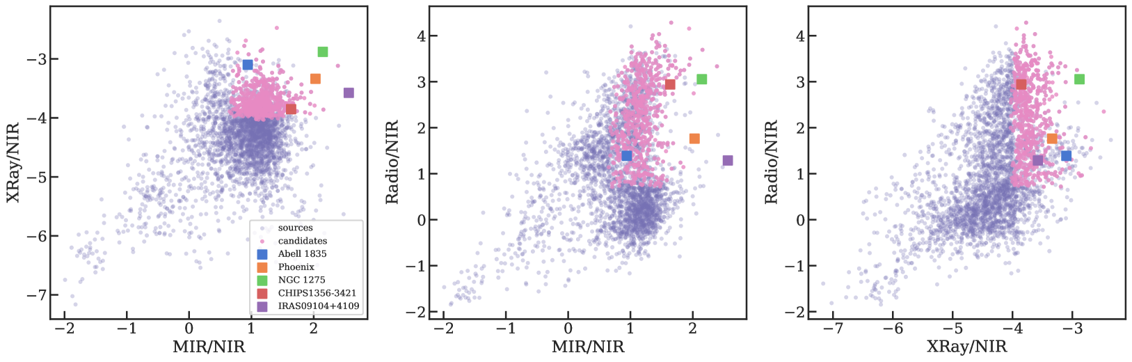
Figure 1.— The three panels show color-color diagrams for objects that are detected in all four all-sky surveys (3,450 objects). The axes are the logarithm of the ratio of the X-Ray, mid-IR (MIR) or radio flux to the near-IR (NIR) flux. Points colored in pink satisfy our three color cuts. The Phoenix, Perseus (NGC 1275), Abell 1835, and IRAS09104+4109 clusters, which host extreme BCGs, are shown with orange, green, blue and purple squares, respectively while CHIPS1356-3421 is shown with a red square.

Further information about our target selection and the first galaxy cluster discovered from this survey, the galaxy cluster surrounding PKS1353-341, are presented in 2018Somboonpanyakul. In the next section, we describe the data used for our optical follow-up of these 470 candidates.

2.2. Optical Follow-up Observations

The optical follow-up program is separated into two parts based on the declination of the targets. Most objects with positive declination are followed up with the Sloan Digital Sky Survey (SDSS) because of its nearly complete coverage in the Northern Sky. Whereas, objects with negative declination are observed with either the first data release of the Panoramic Survey Telescope and Rapid Response System (Pan-STARRS1; 2016Chambers) with sky coverage of declination greater than $-30^{\circ}$ or additional pointed observations using the Parallel Imager for Southern Cosmological Observations (PISCO; 2014Stalder) on the 6.5m Magellan Telescope at Las Campanas Observatory, Chile. Specifically, 256 out of our 470 candidates were observed with SDSS, 64 candidates were observed with Pan-STARRS1, and the remaining 150 candidates were individually observed with PISCO on the Magellan telescope. We note that data from the Dark Energy Survey (DES; 2016DES) was unavailable at the onset of the project. Fig. 2 shows the position of all target candidates in the sky, separated by the telescope used for the follow-up.

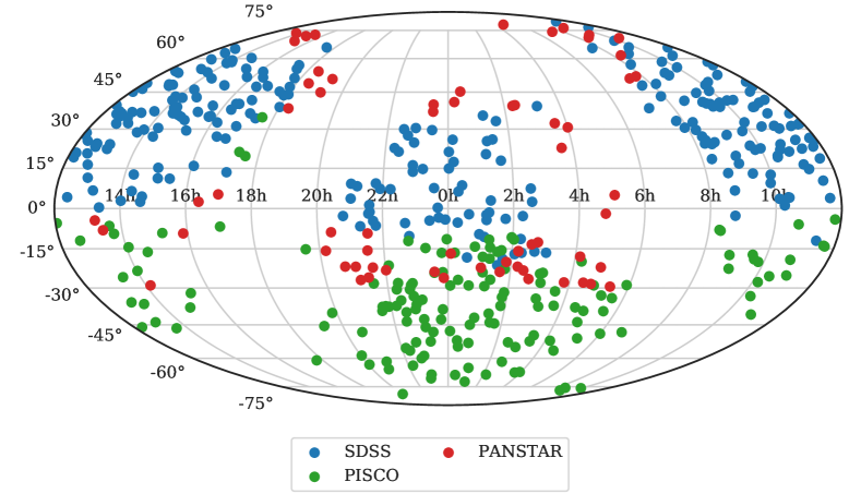
Figure 2.— Plot of all 470 target candidates for the CHiPS survey in the sky. The blue dots represented candidates followed-up with SDSS. The red dots are candidates followed-up with Pan-STARRS, and the green dots are candidates from PISCO observations. The gaps at RA = 18h-20h and 5h-7h corresponds to the Milky Way which prevents us from finding new cluster candidates around that region.

2.2.1 Sloan Digital Sky Survey (SDSS)

The Sloan Digital Sky Survey (SDSS) is a multi-spectral imaging and spectroscopic redshift survey using a 2.5-m optical telescope at Apache Point Observatory in New Mexico (2006Gunn). We utilized Data release 14 (DR14), released in 2017, which is the second data release for SDSS-IV (2018Abolfathi). We retrieved the photometric data in $u$, $g$, $r$, $i$, and $z$ bands by querying objects within a radius of 5 arcmin from the X-ray position, using the function fGetNearestObjEq with the Casjob server. In Section 4, we apply a more stringent cut during the cluster finding algorithm. We obtained the SDSS model magnitude (modelMag) which, as explained in the SDSS support documentation, gives the most unbiased estimates of galaxy colors. To convert SDSS magnitude to flux units, we use the SDSS asinh magnitude formula³, which is also described in (1999Lupton).

For star/galaxy classification, “type” parameters, provided by SDSS, were used to select only galaxies (type = 3). The classification is based on the difference between cmodel and PSF magnitude. Specifically, an object is classified as extended when $\rm{Mag_{PSF}}-\rm{Mag_{cmodel}}>0.145$. In addition, we downloaded photometric redshifts ($z_{\rm{sdss}}$) for photometric redshift estimate verification in Section 4.

2.2.2 Panoramic Survey Telescope and Rapid Response System (Pan-STARRS)

Pan-STARRS is a system for wide-field astronomical imaging in the optical $g$, $r$, $i$, $z$, and $y$ bands, located at Haleakala Observatory, Hawaii. The survey used a 1.8-m telescope, with an imaging resolution of $0.25^{\prime\prime}/\rm{pixel}$ from its 1.4 Gigapixel camera. Pan-STARRS1 (PS1), the basis for Data release 1 (DR1), covers three quarters of the sky ($3\pi$ survey) north of a declination of $-30^{\circ}$.

Star/galaxy separation of PS1 is similar to that of SDSS. Specifically, the difference between model and PSF magnitude is measured to identify extended objects. However, instead of applying a simple straight line as a cut (e.g., $\rm{Mag_{PSF}}-\rm{Mag_{Kron}}>0.05$ where $\rm{Mag_{Kron}}$ is Kron magnitudes as the representation for model magnitude), an exponential model is used to fit the bright part of Fig. 3 and then extrapolated to fainter objects, similar to 2016Chambers. Further details about this technique can be found in 2014Farrow.

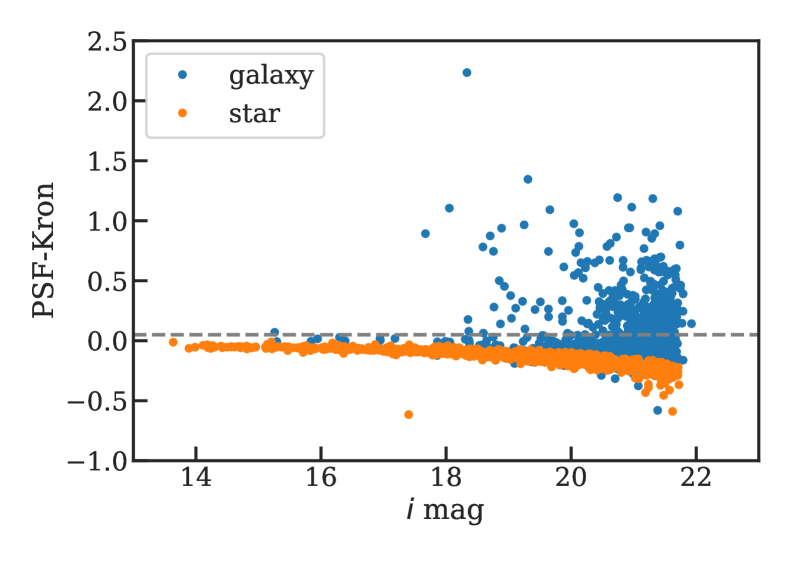
Figure 3.— This figure demonstrates how we separate stars and galaxies in the Pan-STARRS sample catalog using the ratio of PSF and Kron magnitudes. The orange color indicates stars, which pass both the $r$ and $i$ band cut while the blue color marks galaxies.

As shown in Fig. 3, the star-galaxy separation is not a horizontal cut, but an exponential curve which takes into account our inability to distinguish between stars and galaxies at the fainter end. We require the cut to be satisfied for both $r$ and $i$ bands. Even though this star-galaxy-separation criterion could identify more objects as galaxies, this should not create a large bias for our cluster-finding algorithm. We chose Kron magnitudes as the Pan-STARRS magnitudes for our algorithm since they capture more light from the extended parts of galaxies, compared to PSF magnitudes.

2.2.3 Magellan Telescope with PISCO

Without a more robust all-sky survey in the southern sky similar to SDSS and Pan-STARRS in the north, we perform 150 individual follow-up observations for targets in the southern sky with the 6.5-m Magellan telescope. PISCO, a multi-band photometer, is used to speed up our observations because of our large number of candidates. With the ability to produce $g$, $r$, $i$, and $z$ band images simultaneously, our effective efficiency in observing these candidates increases by a factor of $\sim\!3$  (including optical losses; 2014Stalder). All candidates were acquired with PISCO during 9 nights splitting over 3 observing runs between 2017 January to 2017 December. We observed most objects with 5-minute total exposure with two 2.5-minute exposures for dithering. To analyze the PISCO data, we have created a data processing pipeline. Further details regarding data reduction and star/galaxy separation for the CHiPS survey are presented in the next section.

2.3. X-ray Follow-up Observations

To confirm the existence of a galaxy cluster, we require the detection of extended X-ray emission, indicating an extremely hot intracluster medium (ICM), reflecting the deep potential well of the cluster. The Chandra X-ray Observatory is best suited for the task, given that our targets may have bright central point sources. With an angular resolution of 0.5^′′, Chandra has the capability to distinguish X-ray point sources (e.g., AGN) from the extended emission of the ICM. We observed a total of 5 additional candidates from the CHiPS survey, apart from the initial sample of 4 candidates for the pilot study (2018Somboonpanyakul). More details about the reduction process for the X-ray data can be found in Section 5.

3. PISCO Observations and Data Processing

In this section, we describe the data reduction process for the PISCO data. Since we obtain raw images from the PISCO instrument on the Magellan telescope, we developed a complete reduction pipeline to convert these images to photometric catalogs for all galaxies in the field, which are then used as an input for our cluster finding algorithm. In contrast, SDSS and Pan-STARRS are wide-field surveys with available photometric catalogs and, as such, do not require any further data processing.

3.1. PISCO Image Reduction

PISCO is a photometer that produces $g$, $r$, $i$, and $z$ band images simultaneously (2014Stalder). The camera is composed of four 3k$\times$4k charge-coupled devices (CCDs), one for each of the four focal planes, with an un-binned scale of $0.109^{\prime\prime}$ per pixel, resulting in a $5^{\prime}\times 9^{\prime}$ field of view. Each CCD is read out with two amplifiers.

For each image, the data reduction process consists of several steps, as follows. First, the median of all bias frames for each night is subtracted from both the median of all flat frames and the science frames. We do not attempt to quantify and remove the dark current, as it is negligible in these devices. The ratio between the two subtracted frames (flat and science) is the flat-fielded image. The two flat-fielded images (one from each amplifier) of a CCD are stitched together to create a complete image for each band ($g$, $r$, $i$, and $z$) and each exposure. L.A. Cosmic is run on each image for robust cosmic rays detection and removal (2001vanDokkum). Astrometric calibration is carried out via Astrometry.net, which is used to find the absolute pointing, plate scale, orientation, and additional distortions in each image (2010Lang).

Multiple exposures need to be coadded to create a final, stacked image in each band. First, an initial source detection is run on all science images using SExtractor (1996Bertin). Objects which are corrupted or truncated are removed from the lists by requiring the FLAGS parameter to be less than 5. Next, SCAMP (2002Bertin) is run over all of the images simultaneously to improve the astrometric solutions, previously obtained from Astrometry.net. The reference catalog we used for the astrometry is linked to the Two Micron All Sky Survey (2MASS) catalog (2006Skrutskie). The individual images of each band are then resampled and coadded via SWarp (2006Bertin). An example of the final processed image is shown in Fig. 4.

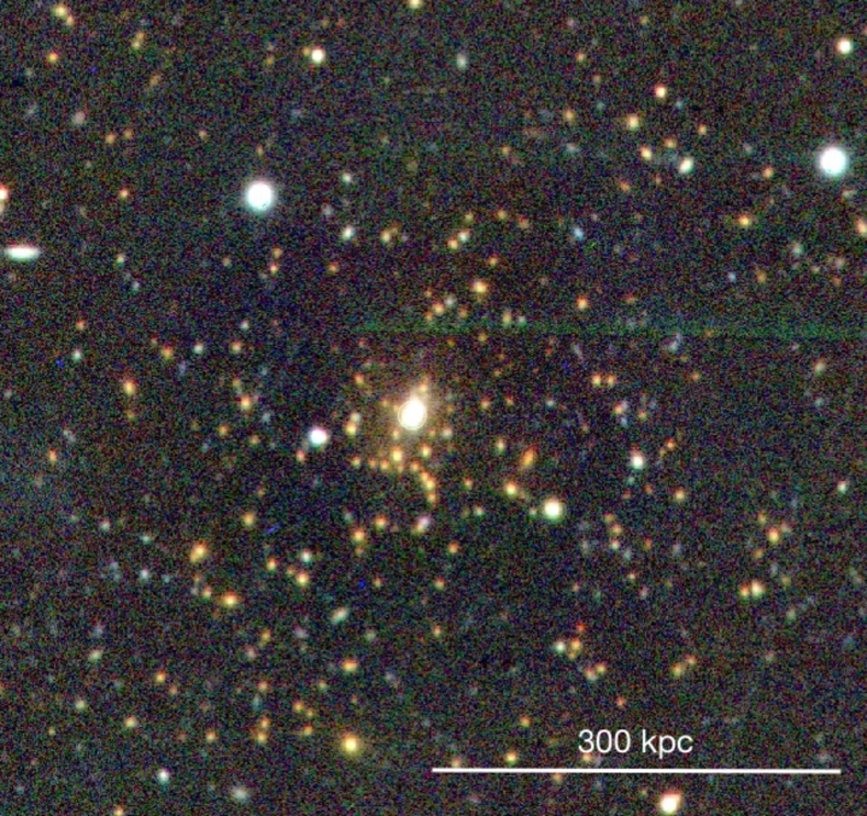
Figure 4.— Three-color ($g$, $r$, $i$) image of the Phoenix cluster from PISCO. The image shows several red galaxies centrally located in the field, which is the signature of a galaxy cluster. The extremely bright point source in the center is a reason why the Phoenix cluster had been missed from previous X-ray surveys.

3.2. Seeing Estimation and PSF Models

Even though each image already has an estimated seeing from the on-site seeing monitor, a more precise value is required for source extraction. We achieve this by fitting the Point Spread Function (PSF) models to every object in the field and picking the most common PSF to represent the seeing of that particular field. Specifically, we create $45\times 45$-pixel small sub-image (“vignettes”) for each detected object by using SExtractor. These small vignettes are fit using the 2D-Moffat model, available in the Astropy model packages (2018Astropy). The Moffat model is a probability distribution that more accurately represents PSFs with broader wings than a simple Gaussian. We quote seeing measurements as the full width at half maximum (FWHM) of the best-fit model. Fig. 5 shows the seeing distribution for objected observed with the PISCO camera. The median seeing in $g$, $r$, $i$, and $z$ bands are $1.^{\prime\prime}28$, $1.^{\prime\prime}15$, $1.^{\prime\prime}14$, and $1.^{\prime\prime}03$ respectively, meaning that the PSF tends to be broader for bluer bands, as expected. For one 2-night run on PISCO, the $r$-band data had a slightly worse (20% larger) PSF due to alignment issues within the instrument. Given that this enlarged PSF is still smaller than that of the SDSS or Pan-STARRS data, we do not expect this to limit our analysis. The seeing distributions are not symmetric, but highly skewed toward higher seeing, representing a variation in the weather at the time of observation.

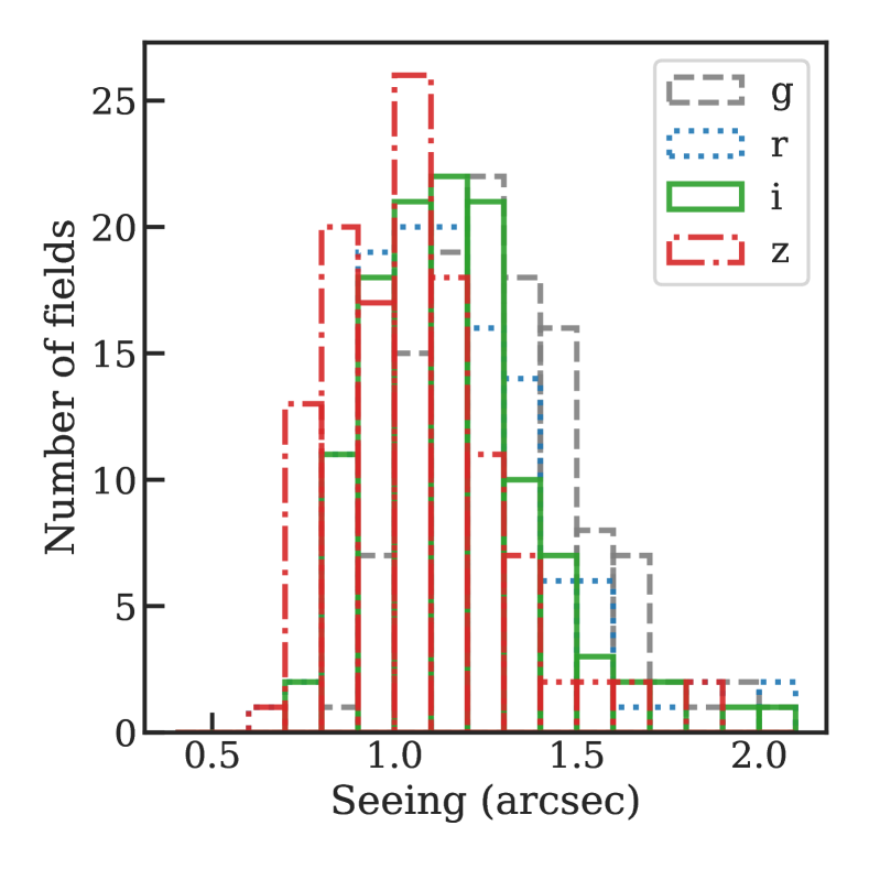
Figure 5.— Seeing distribution for the 262 fields observed with PISCO. The g band is traced by black dashed lines, the r band is traced by blue dotted lines, the i band is traced by green solid lines, and the z band is traced by red dot-dashed lines. The median values of the seeing in g, r, i, z bands are $1.^{\prime\prime}28$, $1.^{\prime\prime}15$, $1.^{\prime\prime}14$, $1.^{\prime\prime}03$ respectively.

Apart from an accurate seeing estimate, the PSF model is also required for SExtractor to measure $\rm{MAG\_PSF}$. We use PSFEx to extract the PSF models from FITS images (2011Bertin), setting all parameters to default. To get a good model for the PSF, we need to only select well-behaved point sources (stars) as our model. We achieve this by selecting sources which are not at the edges of the CCD, not elongated, and have an effective flux radius within $2\sigma$ of the mean for all sources in the field.

3.3. Source Extraction

To measure an accurate color for each object, we extracted photometry via the dual-image mode of SExtractor, which uses the same pixel location for all photometric bands. The seeing estimates and the PSF models are used in this step with other input parameters described in Table 1. Next, we extract $griz$ $\rm{MAG\_AUTO}$, $\rm{MAG\_APER}$, and $\rm{MAG\_PSF}$ at the location of detected sources from the $i$-band image.

Table 1SExtractor Source Detection Input Parameters

Parameter	Value
$\rm{DETECT\_MINAREA}$	$1.1\pi\times(i\,\rm{band\,seeing}^{2})$
$\rm{DETECT\_THRESH}$	1.2
$\rm{GAIN}$	0.25
$\rm{PIXEL\_SCALE}$	0.12 or 0.22
$\rm{SATUR\_LEVEL}$	61,000

3.4. Star-Galaxy Seperation

One of the most important steps for the reduction pipeline is to separate sources into stars and galaxies. While $\rm{CLASS\_STAR}$ is often used for this purpose, upon our close investigation we found non-negligible contamination in both the star and galaxy samples. Instead, we use the $\rm{SPREAD\_MODEL}$ parameter (from SExtractor) which indicates whether the source is better fit by the PSF model or a more extended model (2012Mohr). By design, $\rm{SPREAD\_MODEL}$ is close to zero for point sources and positive for extended sources. This estimator has been used in several surveys, e.g., the Blanco Cosmology Survey (BCS) (2012Desai) and the Dynamical Analysis of Nearby Cluster (DANCe) survey (2013Bouy). In particular, we separate stars and galaxies by the following criteria:

$$galaxies:\rm{SPREAD\_MODEL\_I} >0.005$$ (1)

$$\rm{\&}\,\rm{MAG\_i} <17.5$$

$$stars:\rm{SPREAD\_MODEL\_I} <0.004,$$

where $\rm{MAG\_i}$ is the magnitude of the object in $i$ band. This criteria is adapted from 2018Sevilla-Noarbe, providing a better separation between stars and galaxies, compared to $\rm{CLASS\_STAR}$, because we take into account the PSF variation in the calculation. The exact values of the thresholds are not extremely important since we will later estimate the photometric redshfits ($z_{phot}$) for each object, as shown in Section 4.1. If an object is wrongly identified as a galaxy, we will not obtain a good fit for $z_{phot}$ and the object will be removed from the cluster finding algorithm. More details and different tests to quantify the performance of this star-galaxy statistic can be found in 2018Sevilla-Noarbe.

3.5. Photometric Calibration

To calibrate the color and the magnitudes of stars and galaxies, we use Stellar Locus Regression (SLR; 2009High). SLR adjusts the instrumental colors of stars and galaxies and simultaneously solves for all unknown zero-points by matching them to a universal stellar color-color locus and the known 2MASS catalog. The calibration takes into account difference in instrumental response, atmospheric transparency, and galactic extinction. SLR has been used to calibrate photometry for various surveys including SPT follow-up (2010High) and the Blanco Cosmology Survey (BCS; 2015Bleem). The specific implementation of the algorithm that we utilize here is described in 2014Kelly.

For each frame, we use the stellar sources identified in Section 3.4 as the starting point. We then perform the stellar locus regression, which simultaneously calibrates all optical colors onto the SDSS system. The absolute flux scaling (or zeropoint) is then constrained via the optical-infrared colors from SLR, combined with the 2MASS point source catalog (2006Skrutskie).

3.6. Photometric Verification

We perform a comparison test to check the accuracy of the photometric calibration. The test is carried out by comparing between the colors ($g-r$, $r-i$, and $i-z$) we obtained from the PISCO pipeline and the SDSS colors. To enable this verification, we observed three fields in our SDSS target list with PISCO, reducing the data using the same PISCO pipeline that we have described above. Galaxies found in the SDSS catalog are matched with objects in our observed PISCO frames based on their celestial coordinates. The objects are plotted in Fig. 6, showing the offsets between the color from PISCO and SDSS. The scatter ($\sigma$) of the PISCO colors compared to the SDSS colors is around 0.08–0.14 mag for brighter objects ($16<i_{\rm{PISCO}}<20$), which is as accurate as the calibration between SDSS and Pan-STARRS (2016Chambers).

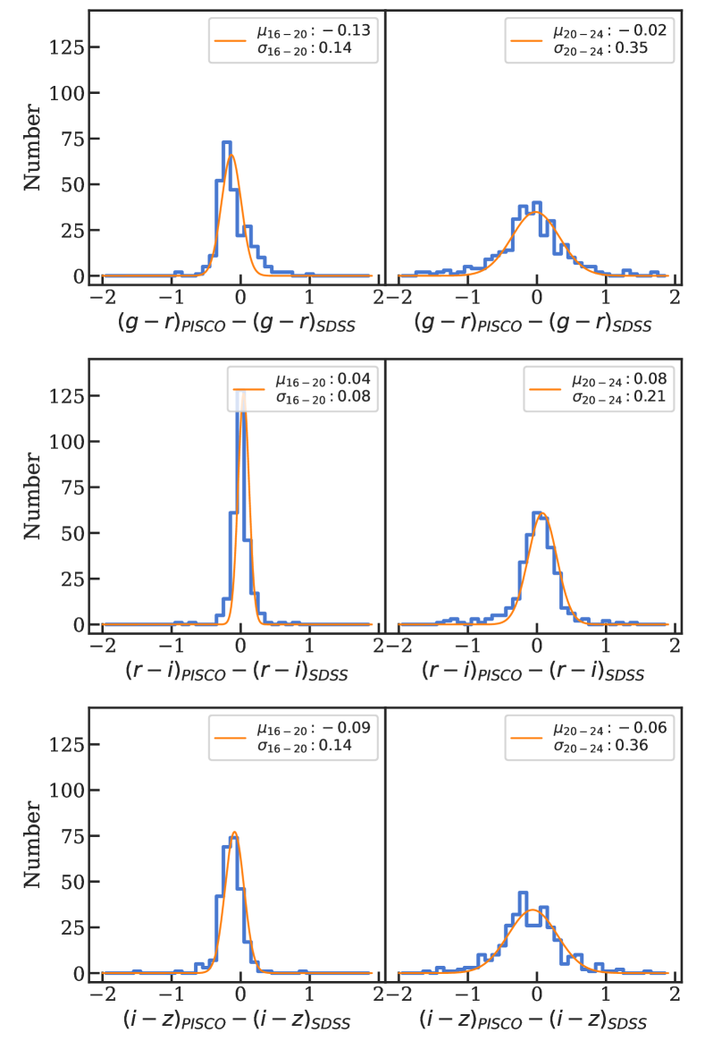
Figure 6.— The top two panels show a comparison of $g-r$ between PISCO PSF magnitude and SDSS PSF magnitude while the middle two show a comparison of $r-i$ and the bottom two show a comparison of $i-z$. The left panels corresponds to bright objects ($16<i_{\rm{PISCO}}<20$) while the right panels corresponds to fainter ones ($20<i_{\rm{PISCO}}<24$). The orange lines are the gaussian best-fit model with its mean and its standard deviation in the legend. This demonstrate that for bright objects, the scatter of the PISCO calibration from the SDSS is about 0.10-0.14 mag.

4. Cluster Finding Algorithm

In this section, we describe the new cluster finding algorithm. Because of the nature of our survey, which looks for cluster candidates surrounding X-ray/IR/radio sources, we already have the central location of the cluster, which we assume to be the location of the X-ray/IR/radio source. This means that unlike some optical cluster finding surveys, we do not use a friend-of-friend algorithm (1982Huchra) to search for the center of the cluster. Instead, we look for an overdensity of galaxies with similar redshifts at the location of the X-ray source.

Specifically, we search for a peak in the redshift histogram of all the galaxies within the observed fields. Members of a galaxy cluster will have similar redshifts, meaning that finding the peak in the redshift histogram will differentiate between cluster members and field galaxies. The peak location corresponds to the redshift of the galaxy cluster.

The algorithm is divided into three parts: photometric redshift measurement, aperture selection and background subtraction, and richness correction for high-redshift clusters.

4.1. Photometric Redshift

The first step of the algorithm is to estimate photometric redshifts of all galaxies in the field. Mid-IR data is included in this step to improve constraints. The sections below describes data acquisition for Mid-IR bands from the Wide-field Infrared Survey Explorer (2010Wright, WISE), and the software used for photometric redshift estimates.

4.1.1 Wide-field Infrared Survey Explorer (WISE)

WISE is an IR satellite with four IR filters, including $W1$ (3.6 $\mu m$), $W2$ (4.3 $\mu m$), $W3$ (12 $\mu m$), and $W4$ (22 $\mu m$). We select galaxies in the AllWISE Source Catalog, using IRSA’s Simple Cone Search (SCS), and match them with their optical counterparts from SDSS, Pan-STARRS, or PISCO within a radius of 3”. However because the FWHM for $W1$ and $W2$ is rather large ($\sim\!6"$, compared to $\sim\!1"$ for optical data), we cannot separate different optical galaxies from the WISE sources, especially at the center of the cluster where large number of objects are presented in a small region. Thus, we only use the WISE measurement from both $W1$ and $W2$ as upper limits to help constrain the photometric redshifts.

4.1.2 Photometric Redshift Estimate

Each galaxy’s photometric redshift ($z_{phot}$) is determined by fitting the photometry in optical and Mid-IR bands to the template spectral energy distribution (SEDs) using the Bayesian Photometric Redshifts (BPZ) code (2000Benitez; 2006Coe). The BPZ code uses Bayesian inference and priors to estimate photometric redshifts using multi-wavelength broad-band data. We used the default templates, consisting of one early-type, two late-type and one irregular-type templates from 1980Coleman and two starburst templates from 1996Kinney. We also added WISE filters for $W1$ and $W2$ band. Since there is no response filter for the PISCO optical bands, we convert the photometry from PISCO to SDSS bands and use SDSS response filters instead. Specifically, we convert the photometry to the SDSS system by fitting a linear function of the form: $(g-r)_{SDSS}=A+B(g-r)_{PISCO}$, and likewise for $r-i$ and $i-z$ colors. This amounts to removing the offset shown in Fig. 6. We apply these corrections to all of the PISCO bands to shift them to the SDSS system. We do not expect the difference in the response filter to have a large impact on the final redshift since PISCO filters are designed to be as similar to the SDSS filters as possible.

4.1.3 Redshift Verification

To verify our photometric redshifts, we compare 612 redshifts from the BPZ algorithm to those publicly available from SDSS3 (2018Abolfathi). In Fig. 7, we show the comparison of BPZ redshifts to those from SDSS3, measuring $\sigma_{z}/(1+z)\sim\!0.05$. The median offset between BPZ and SDSS3 redshifts is $\sim\!0.03$, which is also less than our typical per-galaxy photometric redshift uncertainty. Utilizing 6 previously-known clusters that were identified in our sample (see Section LABEL:sec::known), we also find a scatter between our cluster redshifts and the published values of $\sigma_{z}/(1+z)\sim\!0.012$. Given this overall agreement, we proceed with BPZ redshifts for the full sample.

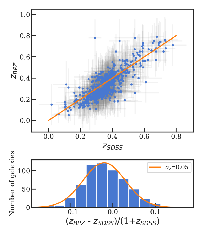
Figure 7.— Comparison between the BPZ redshifts and published photometric redshifts from SDSS3. Most of the objects are in an agreement between the two, with a relative scatter of $\sim\!5\%$.

4.2. Aperture Selection and Redshift Histogram

In terms of aperture selection, we choose a simple top hat model with a radius of one arcminute. This allows us to do a more simple correction for the richness value, as discussed in Section 4.3. Next, we create a histogram representing the redshift distribution of all the galaxies in the selected aperture. Since the peak value includes the background level of field galaxies, we estimate the background distribution by making a redshift histogram of field galaxies in all images of each instrument (SDSS, Pan-STARRS, and PISCO). There are $\sim\!22,000$ background galaxies for PAN-STARRS and PISCO, and $\sim\!27,000$ galaxies for SDSS. We normalized the background histogram for each observation by scaling the total number of objects in the background histogram to be the same as the histogram of interest and subtract from it.

Fig. 8 shows the limiting magnitude for each observation, which demonstrates that the depth of each survey is quite uniform. The detailed calculation for the limiting magnitude is presented in Section 4.3. For PISCO, we made sure that every observation has the same exposure time of 5 minutes. This uniformity allows us to construct the background for each instrument without large variations in limiting magnitude.

The top panel of Fig. 9 shows both the redshift distribution of all the galaxies (in blue) and the normalized distribution of background galaxies (in orange). The background-subtracted histogram is then used to search for a redshift peak, as shown in the bottom panel of Fig. 9. Since the redshifts estimated from the BPZ code have some uncertainty, we fit a fixed-width Gaussian to the peak and the two neighboring bins to get an estimate for the richness (the amplitude of the Gaussian) and the final redshift (the location of the Gaussian).

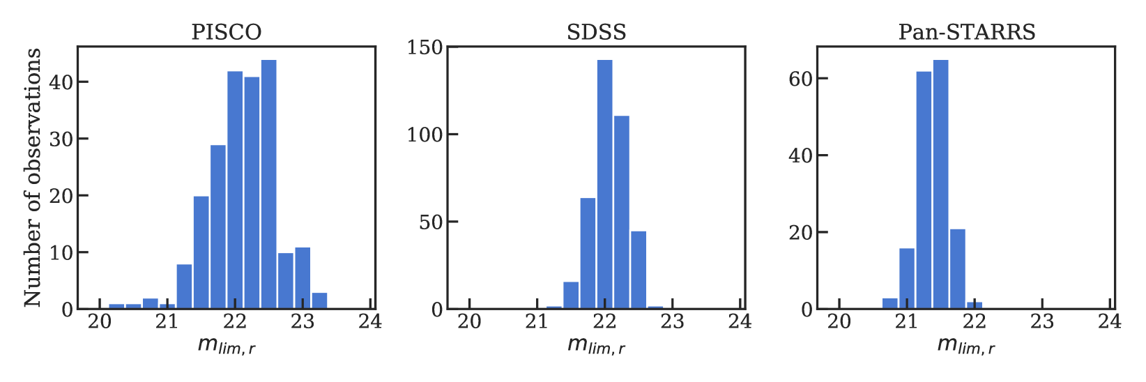
Figure 8.— Limiting magnitude distributions for the three telescopes (PISCO, SDSS, and Pan-STARRS, respectively). This figure shows that the magnitude limit for each telescope is fairly uniform. PISCO has significantly more scatter, compared to SDSS and Pan-STARRS which are wide-field surveys.

Figure 9.— Top: The blue histogram shows the redshift distribution of all the galaxies within one arcmin of CHIPS1911+4455. The orange histogram shows the the renormalized distribution of background galaxies. Bottom: The background-subtracted histogram is shown in blue. The green solid line shows the fixed-width Gaussian fit between the peak and the two neighboring bins to estimate the richness. The significance of the redshift peak at $z=0.53$ strongly suggests the presence of a galaxy cluster.

4.3. Richness Correction

Because observations were made from different optical telescopes and galaxy clusters are located at different redshifts, a correction to the measured richness is necessary to have a uniform proxy for cluster mass across all fields and all redshifts. The two effects we have taken into account include the luminosity function of galaxies and the evolving angular size of galaxy clusters on the sky. We check both effects and find that the luminosity function correction is larger than the angular diameter correction by a factor of $\sim$50–1000, depending on the redshift, so we only consider the luminosity correction.

Extremely bright objects tend to be rare, compared to fainter objects, implying that cluster candidates at higher redshift will have fewer observable members since the majority of them will be too faint to detect with our current instruments. This correction is used to remedy the galaxy counts to account for galaxies that are below detection limits. The luminosity function ($L(M)$) we used comes from 2015Wen which combines the Schechter function $(\phi_{s}(M))$ (1976Schechter) and the composite luminosity function of the BCGs $(\phi_{g}(M))$:

$$L(M)= \phi_{s}(M)+\phi_{g}(M)$$

$$= \>0.4\ln{(10)}\phi_{*}10^{-0.4(M-M_{*})(\alpha+1)}$$

$$\exp{[-10^{-0.4(M-M_{*})}]}$$

$$+\frac{\phi_{0}}{\sqrt{2\pi\sigma}}\exp{\left[-\frac{(M-M_{0})^{2}}{2\sigma^{2}}\right]}dM,$$

where $\alpha$ is the faint-end slope, $M_{*}$ and $M_{0}$ are the characteristic absolute magnitudes, $\phi_{*}$ and $\phi_{0}$ are the normalization factors. Another effect related to the luminosity function comes from variability in the depth of the survey in different field/telescopes. Specifically, SDSS is deeper (fainter limiting magnitude) than Pan-STARRS. Whereas, PISCO has a large variation within itself, which comes from the variation in the weather conditions when we observed these objects. We estimate the limiting magnitude for each observation by fitting two gaussians to the brightness distribution and using the location of the fainter peak to represent the limiting magnitude. The purpose of the double gaussian fit is to capture the skewness in the brightness distribution, which varies from field to field.

Fig. 10 illustrates the richness correction at different redshifts and limiting magnitude ($M_{lim}$). The correction is strongest when we consider high redshift objects with bright limiting magnitudes. The richness is calculated using

$$Richness=N_{obs}\frac{\int^{m_{deep}}_{-\infty}L(M)dM}{\int^{m_{lim}}_{-\infty}L(M)dM},$$ (2)

where $N_{obs}$ is the number of galaxies found from the survey, $m_{deep}$ is the limiting magnitude of our deepest field ($z=0.1$ at a limiting magnitude of 23), and $m_{lim}$ is the magnitude limit of each field. The typical correction is on the order from 1 to 5.

Figure 10.— Richness correction as a function of redshift and limiting magnitude ($M_{lim}$) due to the luminosity function of galaxies where there are fewer bright massive galaxies, compared to faint smaller ones. Specifically, $R_{true}=\frac{R_{obs}}{C(z,M_{lim})}$, where $R_{true/obs}$ is the corrected and measured richness, and $C(z,M_{lim})$ is the richness correction.

4.4. Flux-Limited Nature of Previous Surveys

The CHiPS survey is designed to look for misidentified galaxy clusters in surveys based on data from the ROSAT telescope. One such survey, the ROSAT-ESO Flux-Limited X-ray (REFLEX) Galaxy Cluster Survey (2004Bohringer), contains 447 galaxy clusters above an X-ray flux of $\sim\!3\times 10^{37}\,\rm{erg\,s^{-1}\,Mpc^{-2}}$ (0.1-2.4 keV) which are all spectroscopically confirmed. The left panel of Fig. 11 shows all 447 clusters in the REFLEX sample on an X-ray luminosity ($L_{\rm x}$) vs redshift plot, with the blue line showing the constant flux limit of the REFLEX sample. It is assumed that this survey has found all of the galaxy clusters with luminosities above this limit.

However, some of the X-ray bright point sources detected by ROSAT are believed to be misidentified massive clusters with extreme central galaxies. One of our goals is to find clusters exceeding the REFLEX flux limit but that are classified as point sources. Since obtaining new optical data is more straightforward to obtain compared to X-ray, we convert this REFLEX flux limit to an optical richness limit which can then be used for our richness cut, as described in Section 6.

In order to convert this X-ray flux limit to a richness limit, the optical richness of this sample is required. First, we cross-correlate the REFLEX clusters and SDSS survey, finding 82 clusters that are in both. By running the same cluster finding algorithm as described in this section, we estimate the richness of all 82 REFLEX clusters. Since both the richness and X-ray luminosity are correlated with the total mass of the clusters, we fit a straight line to the log-log plot, as shown in the middle panel of Fig. 11, to find the relation between the flux limit and the richness limit. For the small number of clusters here, and not accounting for selection effects, we measure an intrinsic scatter between richness and X-ray luminosity $\sigma_{ln\lambda|M}=0.33\pm 0.07$, compared to $\sigma_{ln\lambda|M}\sim\!0.46$ from a sample of SDSS redMapper clusters (Murata2018). The last panel of Fig. 11 shows the X-ray flux limit projected onto the richness-redshift plot, via the relationship between richness and X-ray luminosity. Assuming that all clusters follow the same richness–luminosity relation, those systems that lie above this line should have been discovered by the REFLEX survey. In reality, there is significant scatter in the richness–luminosity relation, and those clusters that scatter high in richness at low X-ray luminosity would have been rightfully missed (for example, CHIPS2155-3727).

Figure 11.— Left: the luminosity vs redshift plot for all of the REFLEX clusters with SDSS data. The plot demonstrates the flux-limited nature of the REFLEX survey. The blue line shows the flux limit = $2.5\times 10^{37}\rm{erg/s/Mpc^{2}}.$ The colored dots show three well-known clusters that should have been detected with the ROSAT catalog. Middle: This plot shows a powerlaw relationship between the luminosity from REFLEX clusters and the measured richness from this work. Right: Richness vs redshift plot with constant flux limit. Assuming the luminosity-richness relation from the middle panel, X-ray-selected clusters from the REFLEX catalog should have richnesses that lie above this line.

5. X-ray Data Reduction

In addition to the optical survey, we performed X-ray follow-up of 9 promising candidates with Chandra. Three of them are shown in this work. Four candidates were followed up in Chandra Cycle 16 based on an earlier version of our selection (Somboonpanyakul et al. 2018), which yielded the re-observation of a lesser-known cluster, two systems that turned out to be isolated point sources, and CHIPS1356-3421. In Cycle 20, we followed up an additional 5 candidates, which yielded the detection of CHIPS1911+4455. Both of these follow-up campaigns were based on preliminary catalogs and, thus, had an inflated false-positive rate. In this section, we describe the X-ray data reduction process to estimate the total mass and luminosity of these clusters. A more detailed analysis with these data is described in (2018Somboonpanyakul).

All CHiPS candidates were observed with Chandra ACIS-I for 30-40 ks each. The data was analyzed with CIAO (2006Fruscione) version 4.11 and CALDB version 4.8.5, provided by Chandra X-ray Center (CXC). The event data was re-calibrated with VFAINT mode, and point sources, which are not in the center, were excluded with the wavdetect function. The image was produced by applying csmooth, which adaptively smoothed an image with maximal smoothing scale of 15 pixels and signal-to-noise ratio between 2.5 and 3.5.

High angular resolution X-ray images can be used to estimate different properties of the cluster, including the mass and total luminosity. We choose $M_{500}$, the total mass within $R_{500}$, the radius within which the average enclosed density is 500 times the critical density ($\rho_{c}=3H_{0}^{2}/8\pi G$), to represent the total cluster mass. We use scaling relations from (2009Vikhlinin) iteratively to estimate $R_{500}$, which is then used to measure $T_{\rm x}$, $M_{g}$, and $M_{500}$. Specifically to estimate $M_{500}$, we use the scaling relation with $Y_{\rm x}=M_{g}\times T_{\rm x}$

$$M_{500}= (5.77\pm 0.20)\times 10^{14}h^{0.5}M_{\odot}$$

$$\times\left(\frac{Y_{\rm x}}{3\times 10^{14}M_{\odot}}\right)^{0.57\pm 0.03}E(z)^{-2/5}.$$

$Y_{\rm x}$ is chosen as a mass proxy because of its low scatter and insensitivity to the dynamical state of the cluster (2006Kravtsov; 2009Marrone). More details about the method to estimate $M_{500}$ can be found in 2011Andersson.

In addition to mass, we measure the total X-ray luminosity of each cluster. We first extract an X-ray spectrum of all emission within R500, centered on the X-ray peak, and then we fit this spectrum using a combination of collisionally-ionized plasma (APEC) and Galactic absorption (PHABS). This allows us to estimate the unabsorbed X-ray flux, which we then convert to a rest-frame luminosity given the known redshift.

6. Results

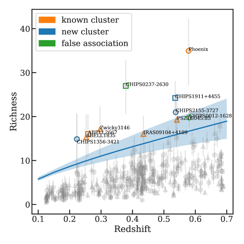
Figure 12.— Richness versus redshift for all CHiPS candidates. The blue solid line shows the richness cutoff we used for the survey (see Fig. 11). Each object is indicated with either a circle, a square, or a triangle based on its optical follow-up telescopes, which are the Magellan telescope (PISCO), Pan-STARRS, or SDSS, respectively. The orange color indicates known clusters above the richness limit, the green color indicates a false association, and the blue color indicates a new cluster candidates. All three of the latter systems have recently-obtained Chandra X-ray follow-up.

From Fig. 12, we identify 11 cluster candidates by selecting all objects above the solid blue line, which is the richness limit derived in Section 4.4. The objects below this line are not necessary all isolated AGNs. They may belong to less massive clusters that fall below our selection threshold – here we only consider very massive clusters that should have been included in surveys such as REFLEX (2004Bohringer) and MACS (2001Ebeling), but were missed due to the presence of an atypical central galaxy.

Using the NASA Extragalactic Database catalog, we search for known clusters within a $3^{\prime}$ radius of the 11 candidates and report, when available, the redshift of known clusters. In Table 6, we present all 11 candidates with their celestial coordinates, richness, measured redshifts, instruments used to detect, and known clusters associated with each system.

Table 2Galaxy cluster candidates/known above the REFLEX flux-limit line in the CHiPS Survey

CHiPS Name	RA	DEC	Richness	$z$	Instruments	Known Cluster	$z_{\rm NED}$	Sep (arcmin)
CHIPS2344-4243	356.18375	-42.72208	34.939	0.579	PISCO	Phoenix	0.596	0.388
CHIPS0237-2630	39.365	-26.5075	26.968	0.379	Pan-STARRS	ABELL0368	0.22	0.395
CHIPS1911+4455	287.75415	44.92222	24.227	0.536	Pan-STARRS	…	…	…
CHIPS2155-3727	328.82791	-37.46361	20.993	0.538	PISCO	…	…	…
CHIPS0012-1628	3.145	-16.46931	19.788	0.581	PISCO	ABELL0011	0.166	3.019
CHIPS1518+2927	229.58292	29.45889	19.249	0.542	SDSS	PSZ1G045.85	0.611	0.197
CHIPS1023+0411	155.91374	4.18819	17.094	0.297	SDSS	Zwicky3146	0.2805	0.145
CHIPS2351-2605	357.91959	-26.08403	16.027	0.258	Pan-STARRS	ABELL2667	0.23	0.025
CHIPS0913+4056	138.44167	40.93903	16.023	0.435	SDSS	IRAS09104+4109	0.442	0.11
CHIPS1401+0252	210.25876	2.88042	15.304	0.253	SDSS	ABELL1835	0.2532	0.055
CHIPS1356-3421	209.023	-34.3531	14.875	0.223	PISCO	…	…