Ideal topological gas in the high temperature phase of SU(3) gauge theory

Abstract

We show that the nature of the topological fluctuations in $SU(3)$ gauge theory changes drastically at the finite temperature phase transition. Starting from temperatures right above the phase transition topological fluctuations come in well separated lumps of unit charge that form a non-interacting ideal gas. Our analysis is based on a novel method to count not only the net topological charge, but also separately the number of positively and negatively charged lumps in lattice configurations using the spectrum of the overlap Dirac operator. This enables us to determine the joint distribution of the number of positively and negatively charged topological objects, and we find this distribution to be consistent with that of an ideal gas of unit charged topological objects.

The presence of topologically nontrivial gauge field configurations is a peculiar feature of QCD that has important phenomenological consequences. Most recently this was highlighted by calculations to estimate the axion mass Borsanyi:2016ksw -Petreczky:2016vrs . An essential ingredient of the calculation was the determination of the temperature-dependence of the topological susceptibility up to temperatures well above the QCD crossover temperature to the quark-gluon plasma.

At very high temperatures, fluctuations of the topological charge are strongly suppressed and occur in the form of localized lumps of action, carrying topological charge $\pm 1$. These objects are probably close in their shape and other properties to solutions of the classical Euclidean gauge field equations, i.e. instantons, or rather their finite temperature counterparts, calorons Kraan:1998pm -Gattringer:2002tg . Moreover, since at high temperatures, fluctuations of the topological charge are strongly suppressed, calorons (and anticalorons) are expected to form a dilute gas and their size is limited by the inverse temperature.

These properties of the caloron gas motivate the so called dilute instanton gas approximation (DIGA) which –in principle– makes it possible to calculate the temperature-dependence of the topological susceptibility perturbatively. However, the topological susceptibility determined in lattice simulations differs by an order of magnitude from the DIGA predictions even at temperatures as high as $5-10T_{c}$ Borsanyi:2016ksw -Petreczky:2016vrs . It is thus clear that at least one of the two assumptions that the DIGA is based on is not satisfied. These two assumptions, both of which are expected to be valid at high enough temperatures are: A1: The probability of one instanton occurring in a given volume can be calculated perturbatively in the semiclassical approximation. A2: The instantons gas is so dilute that interactions among (anti)instantons can be neglected, the gas of topological objects is an ideal gas.

Assumption A1 has been recently reconsidered, but despite the correction of the previously grossly underestimated uncertainty of the semiclassical one-instanton calculation, there is still at least a $3\sigma$ discrepancy between the lattice and the DIGA result for the topological susceptibility Boccaletti:2020mxu . In the present paper we focus on assumption A2 and study interactions among topological objects in the quenched approximation of QCD, just above the finite temperature phase transition. Even apart from the axion problem, a full determination of instanton interactions just above $T_{c}$ is interesting in itself, as it can shed light on how typical gauge field configurations change as the system crosses into the high temperature phase. This might also help us better understand the chiral and deconfining transition in QCD with dynamical quarks.

To see how interactions among instantons could be detected, our starting point is a non-interacting instanton gas. In a free, non-interacting topological gas the number distribution of topological objects can be characterized with a single parameter, the topological susceptibility $\chi=\frac{\langle Q^{2}\rangle}{V}$, where $Q=n_{i}-n_{a}$ is the topological charge (the number of instantons minus the number of antiinstantons), $V$ is the space-time volume and $\langle.\rangle$ denotes the expectation with respect to the path integral. In an ideal topological gas all higher cumulants of the distribution can be exactly calculated in terms of $\chi$. Any deviations from these ideal-gas cumulants are a result of interactions among topological objects.

In the recent literature several quenched lattice calculations of the lowest non-trivial cumulant

$$B_{2}=\frac{\langle Q^{4}\rangle-3\langle Q^{2}\rangle^{2}}{\langle Q^{2}\rangle}$$ (1)

appeared Borsanyi:2015cka ; Bonati:2013tt . The most precise calculation reports that even though above $1.15T_{c}$ the value of $B_{2}$ is consistent with $1$, its ideal-gas value, just above the phase transition, at $1.045T_{c}$ it is still 1.27(7) Bonati:2013tt .

For a more complete assessment of the situation, more information would be desirable about the distribution of the number of topological objects, beyond the first nontrivial cumulant of $Q$. However, higher cumulants of the distribution are notoriously hard to calculate, and even the full topological charge distribution can in principle miss subtle correlations among instantons and antiinstantons. Full information about that is contained only in the joint distribution of the number of instantons and antiinstantons.

The problem is that while there are well-established methods to compute the topological charge $Q=n_{i}-n_{a}$ in lattice simulations, there is no easy way to determine $n_{i}$ and $n_{a}$ separately in lattice configurations. In the present paper we introduce a novel method to compute $n_{i}$ and $n_{a}$ separately, and determine their joint distribution. Our method is based on the low-lying spectrum of the overlap Dirac operator. In particular, our main observation is that mixing instanton-antiinstanton zero modes constitute a distinct part of the Dirac spectrum close to zero, and can be reliably separated from the rest of the spectrum. Counting the number of these close to zero modes together with the exact zero modes of the overlap operator provides a way to determine not only the topological charge $Q$, but also the total number of topological objects $n_{i}+n_{a}$.

Besides yielding much more information than just the cumulant $b_{2}$, our method has another advantage compared to previous studies. By construction it always gives integer numbers, and thereby avoids the ambiguities that plague the definitions of the topological charge based on gauge field operators. In that case, the values of the topological charge are not integers and need to be multiplicatively renormalized, and – if the full charge distribution is needed – also rounded to integers. Higher moments of the distribution, like $b_{2}$ are very sensitive to these ambiguities.

For the present study we used quenched lattice configurations generated at $T=1.045T_{c}$ on lattices of temporal extension $N_{t}=8$ and aspect ratio 3 and 4. For both spatial volumes we determined $n_{i}$ and $n_{a}$ on 5k lattice configurations. In the smaller volume, we found that the number distribution of topological objects significantly deviated from the expectation based on a free non-interacting gas. In contrast, the larger volume showed no such deviation. Although in finite temperature lattice QCD an aspect ratio of 3 is usually considered safe in terms of finite (spatial) volume corrections, we show here that the unexpectedly large finite volume corrections are due to the proximity of the phase transition. We conclude that in quenched QCD already slightly above $T_{c}$ the number distribution of topological objects is consistent with that of a gas of free topological objects.

Let us first motivate the main tool used in our study, the separation of the bulk of the spectrum and the topology-related close to zero modes. It is known that in the presence of an isolated instanton (or antiinstanton) the Euclidean Dirac operator has an exact zero mode with chirality $+1$ ($-1$) Atiyah:rm . In the field of a well separated instanton and antiinstanton the two would be zero eigenvalues split slightly and produce two complex conjugate eigenvalues. The splitting is controled by the spatial distance of the topological objects (relative to their size), as well as their orientation in group space. Generally the farther away the two objects are, the smaller the splitting is, and in the limit of infinite separation the splitting tends to zero Schafer:1996wv . In this way a dilute gas of topological objects is expected to produce not only $|Q|=|n_{i}-n_{a}|$ exact zero modes, corresponding to the net topological charge, but also $n_{i}+n_{a}-|Q|$ small Dirac eigenvalues, from the mixing of opposite chirality instanton and antiinstanton would be zero modes. Motivated by the instanton liquid model, we call the region in the spectrum containing these modes the Zero Mode Zone (ZMZ).

It should be already clear from the above discussion that as the temperature gets higher and topological fluctuations become sparser, the near zero modes of topological origin will be closer to the origin. At the same time, the low end of the bulk of the spectrum, the lowest non-topological modes, controlled by the Matsubara frequency, will move higher as the temperature increases. Therefore, at high enough temperature the ZMZ should be well separated from the bulk of the spectrum. In what follows, we will demonstrate that already slightly above the finite temperature phase transition the ZMZ can be reliably separated from the rest of the Dirac spectrum, provided a chirally symmetric Dirac operator, such as the overlap Narayanan:1993ss is used.

Already in the early days of the overlap it was noticed that above $T_{c}$, besides the expected exact zero modes, the overlap Dirac spectrum also contains an unexpectedly large number of very small close to zero eigenvalues Edwards:1999zm . This enhancement of the low end of the Dirac spectrum resulted in a spike in the spectral density, well separated from the bulk of the spectrum. This came as a surprise, since above $T_{c}$ the restoration of chiral symmetry would imply a vanishing spectral density at zero virtuality, due to the Banks-Casher relation. The spike in the spectral density was conjectured to contain mixing would be zero modes of instantons and antiinstantons. Subsequent work confirmed that this enhancement of the spectral density is neither a discretization, nor a quenched artifact Alexandru:2015fxa . More recently the appearance of this spike in the Dirac spectrum was speculated to signal a genuinely new state of strongly interacting matter, intermediate between the low temperature hadronic and the high temperature quark-gluon plasma state Alexandru:2019gdm .

In the present work we analyze the statistical properties of the eigenvalues in this spike of the spectral density in a high statistics quenched $SU(3)$ lattice study. We show that the statistics of these eigenvalues is to a high precision consistent with the assumption that they are produced by mixing instanton and antiinstanton would be zero modes. To this end we use quenched gauge ensembles generated with the Wilson gauge action at $\beta=6.09$ and temporal lattice extension $N_{t}=8$. This corresponds to a temperature of $T=1.045T_{c}$, just above the finite temperature transition that in the quenched $SU(3)$ case is a first order phase transition. For the detailed statistical analysis we used two ensembles of gauge configurations with spatial extension $L=24$ and $32$, both containing 5000 configurations. In addition, to check finite volume effects in the spectral density and the Polyakov loop distribution, we also had an ensemble of 600 configurations on a larger spatial volume $L^{3}=40^{3}$. The negative mass parameter of the overlap Wilson kernel was set to $M=-1.3$, and two steps of hex smearing Capitani:2006ni were performed on the gauge links before inserting them into the Wilson kernel. The statistical analysis we report here was performed on the overlap Dirac eigenvalues of smallest magnitude with $|\lambda|/T_{c}<2.0$ for all ensembles.

Since we want to compare the statistics of small Dirac eigenvalues with that of non-interacting topological objects, we first summarize our expectations in such an ideal gas of topological objects. In the absence of any interaction among them, both the number of instantons $n_{i}$ and that of antiinstantons $n_{a}$ are expected to follow independent and identical Poisson distributions with mean $V\chi/2$ proportional to the volume, where $V$ is the four-volume of the system and $\chi$ will turn out to be the topological susceptibility. The joint distribution

$$P(n_{i},n_{a})=\mbox{e}^{-V\chi}\frac{(V\chi/2)^{n_{i}+n_{a}}}{n_{i}!n_{a}!}$$ (2)

of $n_{i}$ and $n_{a}$ can be used to compute all the relevant physical quantities of this free topological gas in terms of the single parameter $\chi$. In particular the topological susceptibility is

$$\frac{1}{V}\langle Q^{2}\rangle = \sum_{n_{i}=0}^{\infty}\sum_{n_{a}=0}^{\infty}P(n_{i},n_{a})(n_{i}-n_{a})^{2}=$$ (3)

$$= \overline{n_{i}^{2}}+\overline{n_{a}^{2}}-2\overline{n_{i}}\ \overline{n_{a}}=\chi,$$

where expectations like $\overline{n_{i}}$ are understood to be with respect to the respective Poisson distribution. The topological charge distribution for $Q\geq 0$ is

$$P(Q)=\sum_{n=0}^{\infty}\mbox{e}^{-V\chi}\frac{(V\chi/2)^{Q+2n}}{(Q+n)!n!}=\mbox{e}^{-V\chi}I_{Q}(V\chi),$$ (4)

where $I_{Q}$ are the Bessel functions of imaginary argument. Due to time-reversal symmetry the distribution is symmetric, $P(Q)=P(-Q)$.

Another interesting quantity to consider is the distribution of the total number of topological objects $n=n_{i}+n_{a}$,

$${\cal P}(n)=\sum_{n_{i}=0}^{n}\mbox{e}^{-V\chi}\frac{(V\chi/2)^{n}}{n_{i}!(n-n_{i})!}=\mbox{e}^{-V\chi}\frac{(V\chi)^{n}}{n!},$$ (5)

which is simply a Poisson distribution with mean $V\chi$.

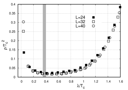
Figure 1: The spectral density of the overlap Dirac operator on quenched $SU(3)$ gauge ensembles just above the phase transition, at $T=1.045T_{c}$. The shaded region indicates $\lambda_{\mbox{\tiny ZMZ}}/T_{c}$, the boundary of the Zero Mode Zone. Eigenmodes below this point in the spectrum are related to mixing topological would be zero modes.

Let us now confront the lattice data with these expectations. In Fig. 1 we show the spectral density of the overlap Dirac operator on the previously mentioned lattice ensembles. Although in the spontaneously broken phase of the pure gauge theory that we consider here, the three Polyakov loop sectors are equivalent, the spectrum of the Dirac operator and the pattern of chiral symmetry breaking/restoration is known to be strongly dependent on the Polyakov-loop sector Gattringer:2002tg , Chandrasekharan:1995gt -Stephanov:1996he . Since in the present work we want to study features that are expected to be at least qualitatively present in QCD with dynamical quarks, here we restrict the analysis to configurations in the physical $\mbox{Re}P>0$ Polyakov loop sector. This is the only one that would be present if dynamical fermions were to be included. In fact, even the slightest explicit breaking of the $Z(3)$ symmetry by dynamical fermions with arbitrarily large, but finite mass would force the system into the real Polyakov-loop sector.

The enhancement of the spectral density near zero is clearly seen in Fig. 1. We note that the exact zero eigenvalues are not shown here, they would appear as a delta function exactly at zero.

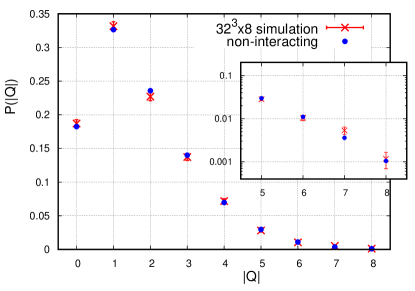
Figure 2: The distribution of the topological charge in our lattice simulations and the distribution expected in a free topological gas with the same susceptibility. As the distribution is expected to be symmetric, positive and negative charges of the same magnitude are counted together. The inset shows the tail of the distribution on logarithmic scale.

Counting the number of zero eigenvalues allows us to compute the topological susceptibility $\chi$, as well as the distribution of the topological charge. In Fig. 2 we compare the distribution obtained in the lattice simulation with the one expected in a free topological gas with susceptibility $\chi$. This is essentially a one-parameter fit of the function in Eq. (4), the fit parameter being $V\chi$ and the chi squared per degree of freedom of the fit turns out to be 0.85.

Encouraged by the good agreement between the lattice data and the free topological gas, we assume that the exact zero modes and the small Dirac eigenvalues, up to a point $\lambda_{\mbox{\tiny ZMZ}}$ in the spectrum, are the eigenvalues associated to the topological objects. In this way, by counting them we count the number of topological objects $n$ present in the gauge field. To make this picture consistent, we have to choose $\lambda_{\mbox{\tiny ZMZ}}$ such that $\langle n\rangle=V\chi$, as predicted by Eq. (5) for an ideal topological gas. Requiring this, results in $\lambda_{\mbox{\tiny ZMZ}}a=0.045(6)$, which turns out to be in the depleted region of the spectral density, separating the spike at zero from the bulk (see Fig. 1). This shows that the ZMZ is indeed well separated from the bulk of the spectrum.

We can now identify the total number of eigenvalues in the zero mode zone, the ones with $|\lambda|<\lambda_{\mbox{\tiny ZMZ}}$ (including the exact zero modes) with $n$, the number of topological objects. Counting the eigenvalues in the ZMZ configuration by configuration, we obtain the distribution of $n$ and in Fig. 3 we compare it with the one expected in a gas of noninteracting topological objects, given by Eq. (5). We emphasize that at this point no fitting is involved, since the only parameter of this distribution, $V\chi$, had already been determined independently from the charge distribution. We do not find a significant deviation from the free topological gas distribution, as the chi squared per degree of freedom of the deviation is 0.62.

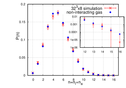
Figure 3: The distribution of the number of topological objects computed from the number of eigenvalues in the zero mode zone. The inset shows the tail of the distribution on logarithmic scale.

We emphasize that the fact that the distribution of the number of eigenmodes of magnitude smaller than $\lambda_{\mbox{\tiny ZMZ}}$ exactly reproduces the distribution we expect from eigenmodes linked to free topological objects is rather non-trivial. By choosing $\lambda_{\mbox{\tiny ZMZ}}$ in the above described manner, we only fixed the expectation of the distribution, and it follows the expected analytical form over three orders of magnitude, the whole range where we have data. This shows not only that the topological objects are indeed non-interacting, but also that already at this temperature the zero mode zone can be reliably separated from the bulk.

So far we determined $\lambda_{\mbox{\tiny ZMZ}}$ from the requirement that the total number of eigenvalues below $\lambda_{\mbox{\tiny ZMZ}}$ (including the zero modes) be consistent with the topological susceptibility obtained by counting the zero modes only. But is $\lambda_{\mbox{\tiny ZMZ}}$ really a special point in the spectrum? To answer this question we chose different cuts in the spectrum and checked how close the distribution of the number of eigenvalues below these cuts are to a Poisson distributions. To this end we determined the distribution of the number of eigenvalues as a function of the cut and for each value of the cut plot the chi squared per degree of freedom of the deviation of the best fit Poisson distribution from the data. In Fig. 4 we show the results. It can be clearly seen that there is a range of cuts $0.3<\lambda_{cut}/T_{c}<0.6$, where the distribution is compatible with Poisson, and the previously independently determined $\lambda_{\mbox{\tiny ZMZ}}$ happens to be in the middle of this range. This further supports that the valley of the spectral density containing $\lambda_{\mbox{\tiny ZMZ}}$ indeed separates the topological modes from the bulk of the spectrum. This valley, however, is rather wide and even though the spectrum there is quite depleted and not many eigenvalues are contained there, the question arises as to how sharply $\lambda_{\mbox{\tiny ZMZ}}$ is defined within the valley. Given the present data set, this question cannot be unambiguously answered. It is possible that with much larger statistics the chi squared test presented in Fig. 4 would further limit the acceptable range for $\lambda_{\mbox{\tiny ZMZ}}$. Another possibility is that in the continuum limit the spectrum could become more depleted in the valley, even a gap could appear there. In that case the exact location of $\lambda_{\mbox{\tiny ZMZ}}$ within the gap would not be important. Finally, it is also possible that even in the continuum limit and with arbitrarily large statistics there would still be some small ambiguity in separating the topological modes and the bulk. To explore these possibilities further would require more extensive simulations that are out of the scope of the present work.

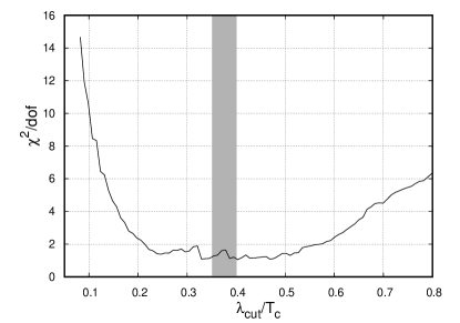
Figure 4: The chi squared per degree of freedom of fits to Poisson distributions of the distribution of the number of eigenvalues with $|\lambda|<\lambda_{cut}$ versus $\lambda_{cut}$. The shaded region shows $\lambda_{\mbox{\tiny ZMZ}}$ with its uncertainty.

The finite temperature $SU(3)$ transition is a first order phase transition, so the correlation length does not diverge, however, large finite volume corrections cannot be excluded. To assess their importance, we repeated the analysis in a smaller volume with linear extension $L=24$. In that case we found significant deviations from the expected free topological gas behavior. The resulting chi squared per degree of freedom was 1.99 and 6.29 in the case of the charge distribution and the distribution of the total number of topological objects, respectively.

Figure 5: The probability distribution of the Polyakov loop for three different spatial volumes with linear size $L=24,32$ and $40$.

To understand finite volume corrections in the vicinity of a phase transition, it is instructive to look at the volume dependence of the distribution of the order parameter. In Fig. 5 we show the probability distribution of the magnitude of the Polyakov loop, the order parameter of the quenched finite temperature transition. Besides the widening of the distribution, expected for smaller volumes, the data for $L=24,32$ lattices also show an unusual enhancement of smaller values of the Polyakov loop. The reason for this is that in the high temperature phase the $Z(3)$ center symmetry is spontaneously broken and the system randomly chooses one of the three $Z(3)$ sectors. However, in a finite volume tunneling among the sectors is still possible, the tunneling probability is enhanced in smaller volumes, and configurations in the process of tunneling have small magnitudes of the Polyakov loop.

As also seen in Fig. 5, in larger volumes these tunneling states get suppressed, however, in smaller volumes they can still give significant contributions to physical quantities, resulting in large finite-size effects. To see, how these tunneling states can affect the topological charge, we looked at the correlation between topology and the Polyakov loop. The simplest quantity to study is the topological susceptibility. We computed its dependence on the Polyakov loop by restricting the averaging of $Q^{2}$ to configurations with Polyakov loop magnitudes in intervals of length 0.01. The results for the $L=24$ and 32 ensembles, shown in Fig. 6, reveal a strong dependence of the susceptibility on the Polyakov loop. The previously seen enhanced contribution of the tunneling region (small Polyakov loop), where the susceptibility is larger, will thus result in significantly larger topological susceptibilities in smaller volumes. To have a feeling about the relative importance of the enhanced region, we note that the probability that $|P|<0.08$ is 0.11, 0.028 and 0.004 for the lattices with linear spatial size size $L=24,32$ and 40 respectively. For the two ensembles shown in Fig. 6 we also indicated the overall susceptibilities and their uncertainties with the horizontal stripes. Since on the $L=24$ lattices even the susceptibility suffers large finite-size effects, it is not surprising that the same occurs for the distribution of the topological charge and the number of topological objects.

We would also like to comment on the apparent discrepancy between our results and those of Ref. Bonati:2013tt who found a significant $(27(7)\%)$ deviation of the $B_{2}$ coefficient from its value (1.0) expected in a non-interacting instanton gas. In fact, our data yields $B_{2}=1.35(41)$, which is compatible with that of the above reference. However, judging from their much smaller uncertainty, their statistics could be more than an order of magnitude larger than ours. Since it is based on the overlap spectrum, our method is computationally much more expensive, and in the present study we could not compete in the statistics, but our method has two advantages. First, it necessarily yields integer charges and avoids the large ambiguity in $B_{2}$ due to any small random fluctuations of the topological charge around integers and the possibly necessary normalization and rounding of the charges. Secondly, our method allows for a full determination of the joint distribution of instantons and antiinstantons. It would be interesting to repeat our calculation using a much larger statistics and to see if there is any deviation in this distribution from that of the number of noninteracting instantons.

In the present paper we used a novel way to compute the joint distribution of the number of topological objects in lattice simulations. We showed that right above the critical temperature of pure $SU(3)$ gauge theory the distribution is consistent with the one expected in an ideal gas of non-interacting charges of unit magnitude. It is remarkable that while below the phase transition topological fluctuations form a dense medium without easily identifiable individual lumps Horvath:2001ir , right above the phase transition an ideal gas of well separated topological lumps emerges. Our result also implies that the most likely explanation of the large discrepancy between the lattice and DIGA based calculation of the topological susceptibility is that the topological lumps we found are not close enough in shape to ideal calorons to warrant a semiclassical treatment.

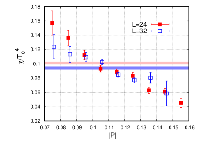
Figure 6: The dependence of the topological susceptibility on the Polyakov loop for two different spatial volumes with linear size $L=24,32$. The two horizontal stripes indicate the susceptibility (with its uncertainty) computed for the full ensembles without restricting the Polyakov loop. The lower value, indicated with the darker band corresponds to the larger volume.

We expect that –at least on a qualitative level– this picture of the topological fluctuations that we found in the quenched case carries over to QCD with dynamical quarks. However, the fermion determinant might introduce some interaction even among well separated topological lumps, but to study that one would need to use a chiral Dirac operator also for the simulation of the sea quarks.

Acknowledgments TGK was partially supported by the Hungarian National Research, Development and Innovation Office - NKFIH grant KKP126769. TGK thanks Matteo Giordano, Sándor Katz and Dániel Nógrádi for helpful discussions.

References

- (1) S. Borsanyi, Z. Fodor, J. Guenther, K. H. Kampert, S. D. Katz, T. Kawanai, T. G. Kovacs, S. W. Mages, A. Pasztor and F. Pittler, et al. Nature 539, no.7627, 69-71 (2016) doi:10.1038/nature20115.
- (2) C. Bonati, M. D’Elia, M. Mariti, G. Martinelli, M. Mesiti, F. Negro, F. Sanfilippo and G. Villadoro, JHEP 03, 155 (2016) doi:10.1007/JHEP03(2016)155.
- (3) P. Petreczky, H. P. Schadler and S. Sharma, Phys. Lett. B 762, 498-505 (2016) doi:10.1016/j.physletb.2016.09.063.
- (4) T. C. Kraan and P. van Baal, Nucl. Phys. B 533, 627-659 (1998) doi:10.1016/S0550-3213(98)00590-2.
- (5) C. Gattringer, M. Gockeler, P. E. L. Rakow, S. Schaefer and A. Schaefer, Nucl. Phys. B 618, 205-240 (2001) doi:10.1016/S0550-3213(01)00509-0.
- (6) C. Gattringer and S. Schaefer, Nucl. Phys. B 654, 30-60 (2003) doi:10.1016/S0550-3213(03)00083-X.
- (7) A. Boccaletti and D. Nogradi, JHEP 03, 045 (2020) doi:10.1007/JHEP03(2020)045.
- (8) S. Borsanyi, M. Dierigl, Z. Fodor, S. D. Katz, S. W. Mages, D. Nogradi, J. Redondo, A. Ringwald and K. K. Szabo, Phys. Lett. B 752, 175-181 (2016) doi:10.1016/j.physletb.2015.11.020.
- (9) C. Bonati, M. D’Elia, H. Panagopoulos and E. Vicari, Phys. Rev. Lett. 110, no.25, 252003 (2013) doi:10.1103/PhysRevLett.110.252003.
- (10) T. Schäfer and E. V. Shuryak, Rev. Mod. Phys. 70, 323-426 (1998) doi:10.1103/RevModPhys.70.323.
- (11) M. F. Atiyah, I. M. Singer, Annals Math. 93 (1971) 139.
- (12) R. Narayanan and H. Neuberger, Phys. Rev. Lett. 71, no. 20, 3251 (1993) doi:10.1103/PhysRevLett.71.3251.
- (13) R. G. Edwards, U. M. Heller, J. E. Kiskis and R. Narayanan, Phys. Rev. D 61, 074504 (2000) doi:10.1103/PhysRevD.61.074504.
- (14) A. Alexandru and I. Horváth, Phys. Rev. D 92, no.4, 045038 (2015) doi:10.1103/PhysRevD.92.045038.
- (15) S. Aoki et al. [JLQCD], [arXiv:2011.01499 [hep-lat]].
- (16) A. Alexandru and I. Horváth, Phys. Rev. D 100, no.9, 094507 (2019) doi:10.1103/PhysRevD.100.094507.
- (17) S. Capitani, S. Durr and C. Hoelbling, JHEP 11, 028 (2006) doi:10.1088/1126-6708/2006/11/028.
- (18) S. Chandrasekharan and N. H. Christ, Nucl. Phys. B Proc. Suppl. 47, 527-534 (1996) doi:10.1016/0920-5632(96)00115-6 [arXiv:hep-lat/9509095 [hep-lat]].
- (19) P. N. Meisinger and M. C. Ogilvie, Phys. Lett. B 379, 163-168 (1996) doi:10.1016/0370-2693(96)00447-9.
- (20) S. Chandrasekharan and S. z. Huang, Phys. Rev. D 53, 5100-5104 (1996) doi:10.1103/PhysRevD.53.5100.
- (21) M. A. Stephanov, Phys. Lett. B 375, 249-254 (1996) doi:10.1016/0370-2693(96)00262-6.
- (22) I. Horvath, N. Isgur, J. McCune and H. B. Thacker, Phys. Rev. D 65, 014502 (2002) doi:10.1103/PhysRevD.65.014502.