An integrated abundance model for estimating county-level prevalence of opioid misuse in Ohio

Abstract

Opioid misuse is a national epidemic and a significant drug related threat to the United States. While the scale of the problem is undeniable, estimates of the local prevalence of opioid misuse are lacking, despite their importance to policy-making and resource allocation. This is due, in part, to the challenge of directly measuring opioid misuse at a local level. In this paper, we develop a Bayesian hierarchical spatio-temporal abundance model that integrates indirect county-level data on opioid-related outcomes with state-level survey estimates on prevalence of opioid misuse to estimate the latent county-level prevalence and counts of people who misuse opioids. A simulation study shows that our integrated model accurately recovers the latent counts and prevalence. We apply our model to county-level surveillance data on opioid overdose deaths and treatment admissions from the state of Ohio. Our proposed framework can be applied to other applications of small area estimation for hard to reach populations, which is a common occurrence with many health conditions such as those related to illicit behaviors.

1 Introduction

The opioid epidemic in the United States is a public health crisis (Office of National Drug Control Policy Executive, Office of the President of the United States, 2011; Drug Enforcement Agency, 2016) associated with unprecedented morbidity and mortality (Rudd et al., 2016; Zibbell et al., 2015). In the 12 month period ending in April 2021, drug overdose deaths in the United States exceeded 100,000, representing a 30% increase from the prior year (CDC, 2021). The opioid epidemic has been particularly severe in Ohio. In 2019, Ohio had the fourth highest overdose death rate of 38.3 per 100,000 which was nearly double the national rate of 21.6 per 100,000 (Division of Unintentional Injury Prevention, 2021). In addition to the epidemic of overdose death, opioid misuse puts Ohio at risk of epidemic levels of Hepatitis C and HIV (Lerner and Fauci, 2019). Knowledge of local prevalence of people who misuse opioids (PWMO) is imperative to quantifying the magnitude of the opioid epidemic. However, this quantity is an unobservable, dynamic subset of the population, and the lack of local estimates of PWMO is a significant barrier to the public health response to the opioid crisis (Schuler et al., 2020).

Despite its importance for guiding a public health response, surveillance of behaviorally-linked conditions, like substance use, is challenging. These conditions tend to vary at the local level and rely on self-reported information, which may not be reliable when dealing with an illicit behavior. This limits the utility of large surveys because they are not typically designed to provide local estimates and are reliant on self-reporting (Palamar et al., 2016). While respondent driven sampling designs (Handcock et al., 2014; Crawford et al., 2018) have been implemented to generate estimates specific to local areas for hard to reach populations, they are typically cross-sectional and would be logistically difficult to implement across larger areas of interest. Thus, there is a great need for local, longitudinal, population-level estimates that cover an entire area of administrative interest, like a state.

In Ohio, the local spatial unit of interest is the county, as that most closely corresponds to the structure of local health districts which form the basis for the allocation of state resources. We lack direct information on the prevalence of PWMO in all of Ohio’s counties. However, we do have indirect information on this quantity in the form of surveillance data collected at the county level. Specifically, we have access to counts of overdose deaths and treatment admissions annually for each county. However, neither surveillance outcome is a perfect reflection of PWMO because there are unique selection processes associated with capturing an individual in either observed outcome that are likely heterogeneous across space and time. For example, overdose death rates are likely related to supply of fentanyl in the local drug market (Pardo et al., 2019). Likewise, treatment admissions are related to local access to care. This heterogeneity prevents us from simply assuming that there is a perfect correlation between the surveillance outcomes and underlying unobservable prevalence of PWMO. Instead, we must explicitly account for these selection processes.

This is structurally similar to the problem faced in ecological applications of estimating population abundance with unmarked observations and unknown detection (i.e., selection) probabilities. Briefly, abundance models use hierarchical models to estimate the total number of individuals in a community when only a proportion can be observed at a given place and time (Royle, 2004; Kery and Royle, 2010). Conceptually, this is also similar to capture-recapture approaches, which have been applied to drug use and HIV in the past (Jones et al., 2016; Bao et al., 2015; Barocas et al., 2018; Min et al., 2020), but does not require identification and tagging of individuals. For our problem, the county-level surveillance outcomes each reflect a proportion of the true population of PWMO in the county whom we are able to observe or detect. Since we lack individual identifying information, we cannot use a capture-recapture approach and instead will consider an extension of abundance modeling to estimate the count and prevalence of PWMO.

One documented challenge with abundance models is the ability to identify intercept parameters for both the latent abundance process and the detection process, which impedes accurate estimates of absolute abundance. Royle (2004) developed an N-mixture model to estimate population size from count data, but identifiability under this approach requires replicated observations of a closed, or unchanging, population. Sólymos et al. (2012) suggested replication is unnecessary provided the number of spatial locations is large and there is at least one continuous covariate that is uniquely related to each distinct process. However, Knape et al. (2015) found that estimates of absolute abundance from an N-mixture model without replication were sensitive to model assumptions on the detection probabilities.

For our application, we lack replication. That is, we do not have repeated observations of a stable population to allow us to uniquely identify both the intercept in the model for the unobserved population in the community and the intercept in the model for the partial proportion of the population observed. Facing a similar problem, Stoner et al. (2019) used informative prior distributions to identify a hierarchical model for under-reporting using a single observed surveillance outcome. While this is a reasonable solution to the problem of non-identifiability when such prior information exists, results will be dependent on the choice of prior (Neath and Samaniego, 1997). Instead, we integrate multiple sources of data at the county and state levels to identify our model. This is the notion behind integrated population models, which are increasingly popular ecological models used to analyze population size. By jointly modeling multiple data sources that share some underlying latent process, these models can allow estimation of parameters which would be non-identifiable in a single outcome model (Besbeas et al., 2002; Schaub and Abadi, 2011). In our setting, the models for the county-level surveillance outcomes of overdose death and treatment counts both relate to the latent number of PWMO. Incorporating multiple county-level surveillance outcomes creates “pseudo-replication” because they show aggregate subsets of individuals who were detected, providing multiple partial views of the population of interest. We also incorporate state-level survey estimates of PWMO to inform the overall statewide prevalence, which, in turn, provides information about the range of the detection probabilities required for identification of the model (Knape et al., 2015). Thus, we use indirect count data on county-level surveillance outcomes and an integrated abundance model framework to inform county-level estimates of PWMO. This can also be viewed as an approach for using the county-level surveillance data to inform small area model-based estimates that downscale the state-level survey data to obtain county-level estimates on PWMO.

In this paper, we develop an extension to the abundance modeling framework that integrates multiple aggregate data sources at different spatial supports to estimate county-level prevalence of PWMO. We define PWMO as those who have misused opioids in the past year and are at risk of experiencing overdose death or treatment admission for opioid misuse. In addition to prevalence and relative risks, we estimate county-level counts of PWMO, which may ultimately be more useful for per capita resource allocation. We will illustrate through simulation studies that our model accurately estimates the quantities of interest and is a drastic improvement over baseline approaches ignoring spatial heterogeneity. We will also illustrate the benefits of including multiple surveillance outcomes. We then apply our methodology to data from Ohio to estimate annual county-level prevalence of PWMO over a 13 year period. By doing so, we provide a coherent framework for integrating multiple sources of data to estimate an unobservable quantity of critical importance for public health policy and resource allocation.

The rest of the paper is organized as follows. We describe the available data in Section 2. The modeling framework is detailed in Section 3. We present the design and results of our simulation study in Section 4. In Section 5, we describe the results for the application to the data from Ohio. We discuss the implications of our findings in Section 6.

2 Data

Since we lack direct county-level data on PWMO, our primary data sources will be annual county-level counts of overdose deaths and treatment admissions for each of Ohio’s 88 counties from 2007-2019, the most recent available year. Overdose death data are publicly available from the Ohio Public Health Data Warehouse (Ohio Public Health Data Warehouse, 2020). Deaths are indexed to the county of residence of the decedent and are counted if the death certificate mentions poisoning from any opioid. Annual county-level treatment admission counts were obtained through a data use agreement with the Ohio Department of Mental Health and Addiction Services. Treatment admissions are indexed to the patient’s county of residence and capture any residential, intensive outpatient, or outpatient treatment for opioid misuse. Data were provided broken down into two age groups (adolescents and adults) but will only be considered in total for this study. State policy requires counts between 1 and 9 to be suppressed, causing some counties to have censored counts. Population data used for calculating rates are estimates from the National Center for Health Statistics and were also obtained from the Ohio Public Health Data Warehouse (Ohio Public Health Data Warehouse, 2020).

Our model also incorporates state-level survey estimates of the prevalence of PWMO from the National Survey on Drug Use and Health (NSDUH) (SAMHSA, Center for Behavioral Health Statistics and Quality, 2003-2005, 2006-2008, 2009-2010, 2011-2014, 2015-2016, 2016-2017, 2017-2018, 2018-2019). We obtain state-level estimates for past year nonmedical opioid use for surveys prior to 2015 and past year opioid misuse after 2015. The language of the survey question was updated in 2015, but we assume the same underlying construct is addressed over time. The survey data for Ohio are estimates of multi-year averages of the statewide prevalence of misuse. The supplementary material contains the multi-year estimates of the statewide prevalence along with the standard errors. Note that the county-level data are from the years 2007 ($t=1$) to 2019 ($T=13$), but we incorporate survey information from 2003 ($t=-3$) to 2019 into the model. The survey estimates are shown in Supplemental Table 1.

We utilize county-level estimates of sociodemographic characteristics from the American Community Survey (ACS) using the R package tidycensus. Variables obtained included poverty rate, unemployment rate, the proportion with at least a high school degree, and the proportion on food stamps. ACS estimates of the 5-year averages are available for all $n=88$ counties in Ohio from 2009 - 2019. ACS estimates for the individual years are available for $38$ of the $88$ counties. We also acquired publicly available data on opioid prescribing rates from the Ohio Automated RX Reporting System (OARRS), which was available from 2010-2019. In addition, we compiled county-level indicators of health professional shortage areas (HPSA) and medically underserved areas (MU) from the Health Resources and Services Administration, high intensity drug trafficking areas (HIDTA) from the Drug Enforcement Agency, and metropolitan statistical areas (MSA) from the United States Census Bureau. We also created an indicator of whether an interstate highway passed through each county to reflect transportation networks.

3 Model

Let $Y_{it}^{(k)}$ be the count of PWMO who experience outcome $k=1,...,K$ in county $i=1,...,n$ during year $t=1,...,T$. Note that in our application, $K=2$ and $k=1,2$ refer to treatment admissions and overdose deaths, respectively. We also observe state-level survey information, denoted $S_{a:b}$, regarding the estimated statewide average prevalence of opioid misuse for the multi-year time period from year $a$ to year $b$ (inclusive). We are ultimately interested in estimating the latent number of PWMO in county $i$ during year $t$, $N_{it}$, and the relative risk of misuse, $\lambda_{it}$. As in Berliner (1996), we use a three-stage Bayesian hierarchical model to relate the observed data to the latent processes of interest. The data, process, and prior layers of the model are defined in the following subsections.

3.1 Data Model

3.1.1 County-level Surveillance Data

We start by specifying a model for the observed county-level surveillance outcomes. Assume

$$Y_{it}^{(k)}|N_{it},p_{it}^{(k)}\stackrel{{\scriptstyle ind}}{{\sim}}\text{Binomial}\left(N_{it},p_{it}^{(k)}\right),$$ (1)

where

$$\text{logit}\left(p_{it}^{(k)}\right)=\mu_{t}^{(k)}+{\bf X}_{it}^{(k)}\mbox{\boldmath$\beta$}^{(k)}+f^{(k)}_{it}+\epsilon_{it}^{(k)}.$$

In the logistic regression model for each outcome $k$, $\mu_{t}^{(k)}$ is a time varying intercept, ${\bf X}_{it}^{(k)}$ is a vector of centered covariates, $\mbox{\boldmath$\beta$}^{(k)}$ is a vector of regression coefficients, $f^{(k)}_{it}$ is a spatio-temporal random effect, and $\epsilon_{it}^{(k)}\overset{iid}{\sim}N(0,\sigma^{2}_{k})$ accounts for additional unexplained heterogeneity. We assume that each surveillance outcome is conditionally independent given the underlying true number of PWMO. That is, we assume marginal dependence between the counts within a county is attributable to the number of PWMO in that county. For our application, the design matrix for treatment rate ${\bf X}^{(1)}$ contains indicator variables that identify the counties that are classified as HPSA and MU. The design matrix for death rate ${\bf X}^{(2)}$ contains indicator variables for whether or not the county contains an interstate, whether the county is a HIDTA, and whether the county belongs to a MSA.

As mentioned in Section 2, the age-group specific treatment counts are suppressed if they are between 1 and 9. However, we can incorporate the knowledge that suppressed counts are within that interval into our model by adapting the approach of Famoye and Wang (2004) for interval censoring. There are three cases of censoring that we encounter here, denoted by the indicator:

$$c_{it}=\begin{cases}0&\text{total count observed}\\ 1&\text{adolescent count censored}\\ 2&\text{adolescent and adult counts censored}.\end{cases}$$ (2)

For $c_{it}=0$, we observe both the adult and adolescent counts and so the total treatment count is their sum. For $c_{it}=1$, we observe the adult count, but the adolescent count is censored so we know that the total count must be between the adult count plus 1 and the adult count plus 9. Finally, for $c_{it}=2$, both counts are censored so we know the total count must be between 2 and 18. Let $Y^{(1)}_{it0}$ be the adolescent treatment count and $Y^{(1)}_{it1}$ be the adult treatment count. Then, we have

$$Y^{(1)}_{it}=\begin{cases}Y^{(1)}_{it0}+Y^{(1)}_{it1}&c_{it}=0\\ Y^{(1)}_{it1}&c_{it}=1\\ 0&c_{it}=2,\\ \end{cases}$$ (3)

and the likelihood from Equation 1 becomes

$$L(\mathbf{p}^{(1)},\mathbf{p}^{(2)},\textbf{N}|\textbf{Y}^{(1)},\textbf{Y}^{(2)})=\left[\prod_{t=1}^{13}\prod_{i=1}^{88}f\left(Y_{it}^{(2)}|p_{it}^{(2)},N_{it}\right)\right]\times$$

$$\times\left[\prod_{t=1}^{13}\prod_{i=1}^{88}\left[f\left(Y_{it}^{(1)}|p_{it}^{(1)},N_{it}\right)\right]^{I(c_{it}=0)}\left[F\left(Y_{it}^{(1)}+9|p_{it}^{(1)},N_{it}\right)-F\left(Y_{it}^{(1)}|p_{it}^{(1)},N_{it}\right)\right]^{I(c_{it}=1)}\right.$$ (4)

$$\hskip 14.45377pt\times\left.\left[F\left(18|p^{(1)}_{it},N_{it}\right)-F\left(1|p^{(1)}_{it},N_{it}\right)\right]^{I(c_{it}=2)}\right]$$

where $F\left(\cdot|p^{(1)}_{it},N_{it}\right)$ is the cumulative distribution function and $f\left(\cdot|p^{(1)}_{it},N_{it}\right)$ is the probability mass function of the binomial distribution with population size $N_{it}$ and rate $p^{(1)}_{it}$, and $f\left(\cdot|p^{(2)}_{it},N_{it}\right)$ is the probability mass function of the binomial distribution with population size $N_{it}$ and rate $p^{(2)}_{it}$.

3.1.2 State-level Survey Data

For the survey information regarding overall statewide prevalence of misuse between years $a$ and $b$, given by $S_{a:b}$, we assume a normal distribution truncated to $(0,1)$. The standard error $\hat{se}_{a:b}$ is estimated from the survey and assumed to be known. We assume a truncated normal distribution to enable the direct incorporation of the mean and standard error reported from the survey. In addition, we let $\mu_{t}$ denote the true latent statewide prevalence of misuse in year $t$ and assume this is linear over time such that $\mu_{t}=\beta_{0}^{\mu}+\beta_{1}^{\mu}t$. Note that this formulation requires survey data to be observed for at least two time periods. More specifically, we assume

$$S_{a:b}|\beta_{0}^{\mu},\beta_{1}^{\mu}\sim N_{(0,1)}\left(\frac{1}{b-a+1}\sum_{t=a}^{b}\mu_{t},\hat{se}_{a:b}^{2}\right),$$ (5)

so that the mean of $S_{a:b}$ is the mean of the true statewide prevalence during the time period from a to b. The linearity assumption for $\mu_{t}$ implies the mean function is

$$\frac{1}{b-a+1}\sum_{t=a}^{b}\mu_{t}=\beta_{0}^{\mu}+\beta_{1}^{\mu}\frac{1}{b-a+1}\sum_{t=a}^{b}t=\beta_{0}^{\mu}+\beta_{1}^{\mu}\frac{b^{2}+b-a^{2}+a}{2(b-a+1)}.$$

We assume survey estimates are independent of one another, conditional on the true statewide rate of misuse.

3.2 Process Model

We are primarily interested in estimating the latent number of PWMO, $N_{it}$, and the relative risk of misuse, $\lambda_{it}$. We assume a non-canonical, spatial rates-like parameterization (Cressie et al., 2005; Cressie and Wikle, 2011):

$$N_{it}|\lambda_{it}\stackrel{{\scriptstyle ind}}{{\sim}}\text{Binomial}(P_{it},\mu_{t}\lambda_{it}),$$

where $P_{it}$ is the known population of county $i$ during year $t$. Let $\lambda_{it}$ represent the relative risk of misuse in county $i$ during year $t$ compared to a statewide average prevalence, $\mu_{t}$, subject to the constraint $0<\mu_{t}\lambda_{it}<1$. Recall, $\mu_{t}$ is assumed to be linear across time and is informed by survey data, as described in Section 3.1.2. We use a non-standard parameterization because the survey data reflects a state average which is not equivalent to the intercept of a standard logistic regression. Note that we could also consider a Poisson model for the latent counts. The large population size and small rates of misuse imply these models will yield near identical results. We chose a binomial model to explicitly allow for the known population size, $P_{it}$.

Assume $\log(\lambda_{it})=\mathbf{W}_{it}\boldsymbol{\gamma}+u_{it}+v_{it}$, where $\mathbf{W}_{t}$ is a design matrix for time $t$ containing centered covariates without an intercept, $u_{it}$ is a spatio-temporal random effect, and $v_{it}\overset{iid}{\sim}N(0,\sigma^{2}_{v})$. For the spatio-temporal random effect $u_{it}$, we assume an intrinsic conditional autoregressive (ICAR) model with an autoregressive of order one (AR(1)) temporal trend (Besag, 1974). More specifically, this model assumes for $t=1$

$$u_{it}|\mathbf{u}_{-i,t},\tau^{2}_{u}\sim N\left(\frac{1}{w_{i+}}\sum_{j}w_{ij}u_{jt},\frac{\tau^{2}_{u}}{w_{i+}}\right),$$ (6)

and for $t=2,...,T$

$$u_{it}|\mathbf{u}_{-i,t},u_{i,t-1},\tau^{2}_{u},\phi_{u}\sim N\left(\phi_{u}u_{i,t-1}+\frac{1}{w_{i+}}\sum_{j}w_{ij}(u_{jt}-\phi_{u}u_{j,t-1}),\frac{\tau^{2}_{u}}{w_{i+}}\right),$$ (7)

where $\mathbf{u}_{-i,t}=\{u_{jt}:j\neq i\}$, $w_{ij}$ is an indicator that counties $i$ and $j$ share a border, and $w_{i+}=\sum_{j}w_{ij}$ is the total number of neighbors for county $i$. Let $\mathbf{u}_{t}=\left(u_{1t},...,u_{nt}\right)^{\prime}$ denote the vector of random effects during year $t$. The intrinsic models specified by equations (6) and (7) yield joint distributions with probability density functions

$$\left[\mathbf{u}_{1}|\tau^{2}_{u}\right] \propto\exp\left(-\frac{1}{2\tau^{2}_{u}}\mathbf{u}^{\prime}_{1}(\mathbf{H}-\mathbf{A})\mathbf{u}_{1}\right)\text{ for }t=1$$

$$\left[\mathbf{u}_{t}|\mathbf{u}_{t-1},\tau^{2}_{u},\phi_{u}\right] \propto\exp\left(-\frac{1}{2\tau^{2}_{u}}\left(\mathbf{u}_{t}-\phi_{u}\mathbf{u}_{t-1}\right)^{\prime}(\mathbf{H}-\mathbf{A})\left(\mathbf{u}_{t}-\phi_{u}\mathbf{u}_{t-1}\right)\right)\text{ for }t=2,...,T,$$

where $\mathbf{A}$ is the adjacency matrix whose $(i,j)$th element is $w_{ij}$ and $\mathbf{H}$ is a diagonal matrix with $(i,i)$th element $w_{i+}$. The above are not valid probability densities since the precision $\mathbf{H}-\mathbf{A}$ is less than full rank. However, the ICAR model is a valid process level model provided a centering constraint, $\sum_{i}u_{it}=0$ for all $t,k$, is enforced (Banerjee et al., 2004).

In this application, we chose to include standardized county-level covariate information on poverty rate, unemployment rate, the percentage with at least a high school degree, the percentage on food stamps, and the opioid prescribing rate per capita as covariates for relative risk of misuse. The prescribing rate data from OARRS is only available from 2010 to 2019. Thus, this variable is only included in $\mathbf{W}_{t}$ for $t=4,...,T$.

As discussed in Section 1, it is well known that the single visit abundance model suffers from non-identifiability of intercept parameters. To see this more clearly, one can show that in the single outcome ($K=1$) case, integrating out the latent count $N_{it}$ yields the marginal distribution $Y_{it}^{(k)}|p_{it}^{(k)},\mu_{t},\lambda_{it}\sim\text{Binomial}(P_{it},\mu_{t}\lambda_{it}p_{it})$. The product form for the rate implies these quantities, and in particular the intercept parameters $\mu_{t}$ and $\mu_{t}^{(k)}$, cannot be individually identified without additional information. However, our model’s integration of multiple data sources eliminates this issue. In particular, the survey data directly informs $\mu_{t}$. Also note that by jointly modeling $K>1$ outcomes, the joint marginal distribution of the outcomes after summing over the possible values of $N_{it}$ does not take the same simple marginal form that results with the single outcome setting. By proposing an integrated model that jointly models multiple data sources, we are able to identify the primary quantities of interest, $N_{it}$ and $\lambda_{it}$. Achieving identifiability by integrating multiple data sources is discussed in Besbeas et al. (2002) and Section 9.2 of Cole (2020).

The models for the surveillance outcomes depend on spatio-temporal random effects $f_{it}^{(k)}$. These are specified similarly to the spatio-temporal random effects in the process-level model for the relative risk of misuse. In particular, for each outcome $k$, we assume an ICAR model with an AR(1) temporal trend analogous to (6)-(7) with conditional variance parameter $\tau^{2}_{k}$ and temporal autocorrelation parameter $\phi_{k}$. We assume these random effects are independent across the $k$ outcomes. In more traditional models, we would expect these rates to be correlated within a county because they share a common underlying process, the latent number of PWMO in that location. However, we explicitly account for that process as the outcome models are specified conditional on the latent number of PWMO so that these random effects capture residual spatial variability in the outcome-specific rates of opioid overdose death and treatment admissions. We a priori do not believe these conditional rates would follow similar spatial trends. If instead we were modeling outcomes that were believed to be correlated conditional on $N_{it}$, this model can easily be generalized to a multivariate conditional autoregressive model.

3.3 ACS Covariate Model

Our process model relates the relative risk of misuse, $\lambda_{it}$, to centered covariates from the ACS in the design matrix ${\bf{W}}_{t}$. However, only 5-year average estimates are available for all 88 counties, which leads to temporal misalignment with the annual estimates of interest. To account for this and the additional uncertainty from using multi-year average estimates, we add an additional layer to the data and process stages of the model, similar to the work of Bradley et al. (2015), to account for uncertainty in the latent yearly county-level values of these variables. This additional layer leverages the annual estimates that are available in 38 counties to inform the latent annual value in counties where only 5 year average estimates are available.

Let $\hat{\omega}_{it}^{(5)}$ and $\hat{\omega}_{it}^{(1)}$ denote the $5$-year and $1$-year estimates from the ACS for one of the variables of interest with standard errors $\hat{\sigma}_{(5)}$ and $\hat{\sigma}_{(1)}$, respectively. Let $\omega_{it}$ denote the true latent value of this variable in county $i$ during year $t$. The columns of the design matrix $\mathbf{W}_{t}$ corresponding to the ACS variables contain standardized variables and are thus functions of these latent $\omega_{it}$. For $t=3,...,T$ and each of the ACS variables included, we assume

$$\hat{\omega}_{it}^{(5)} \sim N_{(0,100)}\left(\frac{1}{5}\sum_{\ell=t-4}^{t}\omega_{i\ell},\hat{\sigma}_{(5)}^{2}\right)$$ (8)

$$\hat{\omega}_{it}^{(1)} \sim N_{(0,100)}\left(\omega_{it},\hat{\sigma}_{(1)}^{2}\right),$$

where $N_{(0,100)}$ denotes the normal distribution truncated to $(0,100)$ since our variables of interest are recorded as percentages. Observe that even though we only include ACS estimates from 2009 - 2019, we infer latent values of the yearly variables from 2005 - 2019.

In the process level of the model, we assume the latent yearly percentages follow $\omega_{it}\overset{ind}{\sim}N_{(0,100)}\left(\omega_{t},\tau_{i}^{2}\right)$, where $\omega_{t}$ denotes a statewide average for that variable in year $t$. This community-level process model for the latent variables permits some borrowing of strength across the counties, improving estimation in the counties that only have $5$-year estimates available. We note that a more complicated spatio-temporal structure could be considered here as was done in Bradley et al. (2015), but it comes with additional computational expense.

3.4 Prior Model and Posterior Distribution

All intercepts and regression coefficients, $\mu_{t}^{(k)},\mbox{\boldmath$\beta$}^{(k)},\beta_{0}^{\mu},\beta_{1}^{\mu},$ and $\boldsymbol{\gamma}$, are independently assigned flat, uniform prior distributions on the real line. The statewide average yearly percentages for the ACS variables, $\omega_{t}$ are assigned a uniform prior distribution over $(0,100)$. All variance parameters $\sigma^{2}_{k},\tau^{2}_{k},\tau^{2}_{u},$ $\sigma^{2}_{v}$, and $\{\tau^{2}_{i}\}$ are assumed to have inverse gamma prior distributions with shape and scale parameters of 0.5. The temporal autoregressive parameters $\phi_{k},\phi_{u}$ are assumed to be uniform over $(0,1)$. The posterior distribution of the latent processes and parameters is simulated using an adaptive Metropolis-within-Gibbs Markov chain Monte Carlo (MCMC) algorithm implemented using the R package NIMBLE (de Valpine et al., 2017). To improve the efficiency associated with sampling highly correlated variables, for each county $i$, the latent counts $N_{i1},...,N_{iT}$ are updated jointly using an automated factor slice sampler as in Stoner et al. (2019). NIMBLE enforces the zero mean constraint in the ICAR models with a commonly used approach of updating these variates without the constraint and then centering (Paciorek, 2009). Convergence of the Markov chain was assessed by visually inspecting trace plots. The R code is included in the supplementary material.

4 Simulation Study

We performed a simulation study to assess the proposed model’s ability to accurately predict latent counts of misuse, $N_{it}$, and relative risk $\lambda_{it}$. We fixed values of all hyperparameters and simulated $M=100$ latent processes and data sets from the proposed model where each data set consisted of $T=10$ years of data for each of $n=100$ counties on a $10\times 10$ grid for $K=2$ county level outcomes and also yearly survey estimates of statewide prevalence. This mimics the setting for the Ohio data we consider in Section 5 where the county-level outcomes correspond to treatment admission counts ($k=1$) and death counts ($k=2$). Note that for the purpose of the simulation, we assume the survey estimates are yearly and not multi-year averages, and we assume covariates used in the design matrix $\mathbf{W}$ are known so no process-level model is needed for these values. Specific details regarding how the data were simulated are in the Supplementary Material.

For each of the $M=100$ simulated data sets, we fit the proposed model under two scenarios: (1) assuming we observed yearly survey information and (2) assuming we only observed survey information in years $2,5,8$, which we will refer to as the sparse survey information scenario. These cases reflect a slightly better and slightly worse case than the actual multi-year average survey data that is available for the application. We will compare the results of our proposed joint model to a baseline model that assumes the state-level survey estimate applies to all counties (Rembert et al., 2017; Burke and Buchanich, 2018) (i.e., no spatial heterogeneity such that $\hat{N}_{it}=\hat{\mu}_{t}P_{it}$) and to a model using only a single county-level outcome (e.g. death counts) (Stoner et al., 2019). We used the R package NIMBLE to run a MCMC algorithm for each of the $M$ data sets under each scenario.

To assess performance, we used the posterior mean as our estimate of latent misuse, $\hat{N}_{it}$, for each simulated data set and computed 95% equal-tail credible intervals. We used several different criterion to assess how well each approach estimated the true latent counts $N_{it}$ and relative risk $\lambda_{it}$. We computed the coverage probabilities (CP) of the credible intervals for the latent counts, the root mean squared error (RMSE) of the counts and of the relative risk, as well as the relative median absolute error (MAE) for the counts.

4.1 Simulation Results

Table 1: A comparison of results from the proposed joint model to the baseline model. The first two columns show the mean and median coverage probability (CP) across the 100 simulated data sets for $N_{it}$ (proposed/baseline). The final three columns present the proportion of simulated data sets for which the proposed model results in a smaller error along with the average error across the 100 data sets for each model (proposed/baseline).

Survey Mean CP Median CP RMSE ($N_{it}$) RMSE ($\lambda_{it}$) Relative MAE ($N_{it}$) Yearly 95% 96% 100/100 100/100 100/100 2598/5581 0.29/0.64 0.16/0.32 Sparse 93% 95% 100/100 100/100 100/100 2890/5647 0.29/0.64 0.17/0.33

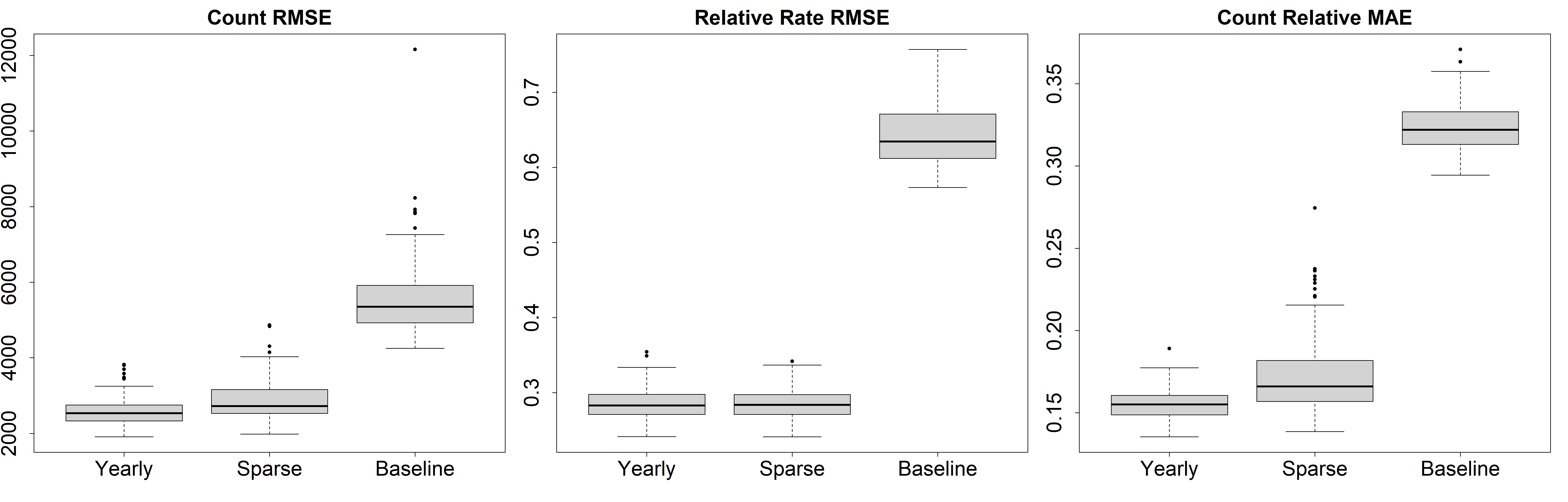
Figure 1: Boxplots of the RMSE for the counts ($N_{it}$) (left) and relative risk ($\lambda_{it}$) (middle) and the relative MAE for the counts ($N_{it}$) (right) for the 100 simulated data sets under the proposed joint model assuming yearly survey data, the proposed joint model assuming sparse survey data, and the baseline estimates based on yearly survey data.

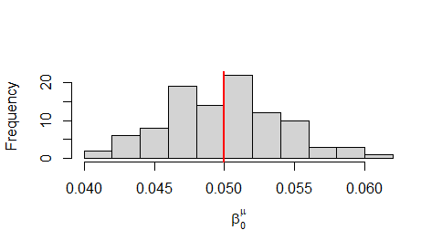
(a) $\beta_{0}^{\mu}$

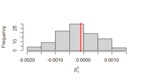
(b) $\beta_{1}^{\mu}$

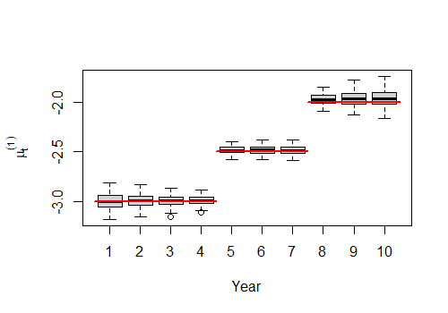
(c) $\mu_{t}^{(1)}$

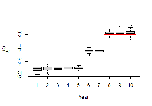
(d) $\mu_{t}^{(2)}$

Figure 1: Plots of the estimates of the intercept parameters for the $H=100$ simulated data sets. The vertical red lines correspond to the true values used to simulate the data.

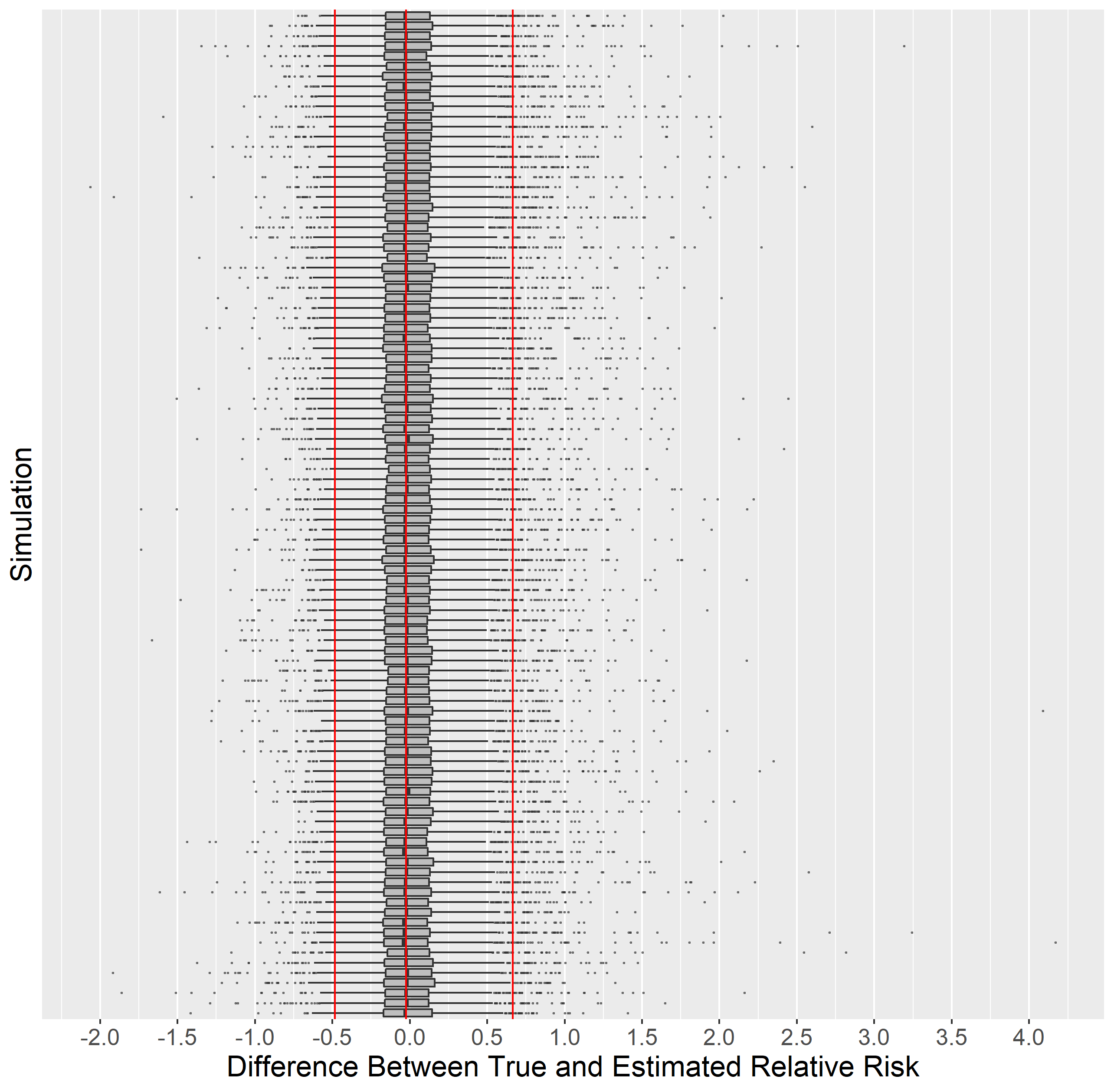
(a) Absolute Difference

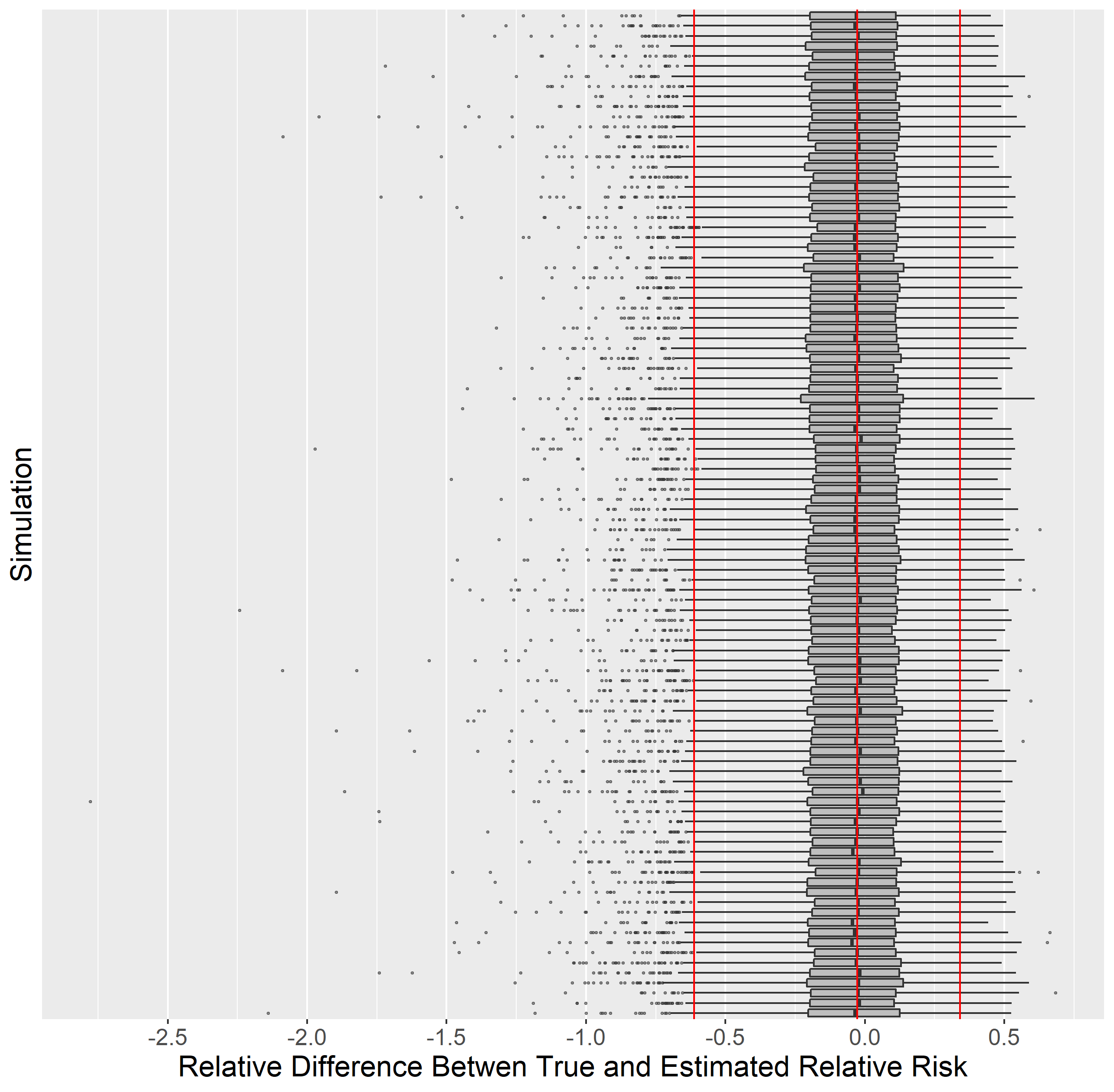
(b) Relative Difference

Figure 2: Boxplots of the absolute and relative difference between the estimate of $\lambda_{it}$ and the true simulated value for each location in each of the $H=100$ simulated data sets. Vertical red lines correspond to the first quartile, median, and third quartile across all of the simulated data sets.

The main findings of the simulation study are summarized here with additional results in the supplementary material. Briefly, the error rates of the proposed model were roughly half that of the baseline model for both the yearly and sparse survey scenarios, with these quantities smaller for the yearly survey information setting compared to the sparse survey setting (Table 1 and Figure 1). The average coverage probabilities of the credible intervals were very close to the target value of 95%. We also compared the results of our proposed joint model to the model that only considers a single county-level outcome ($Y_{it}^{(2)}$) in addition to the survey data for both the yearly and sparse survey data cases. The proposed joint model yields a coverage probability that is closer to 95% than would be obtained modeling just a single county-level outcome. We also see that the proposed joint model yields smaller errors for almost all of the 100 simulated data sets, with the average error reduced by at least 20% (Table 2 and Figure 2).

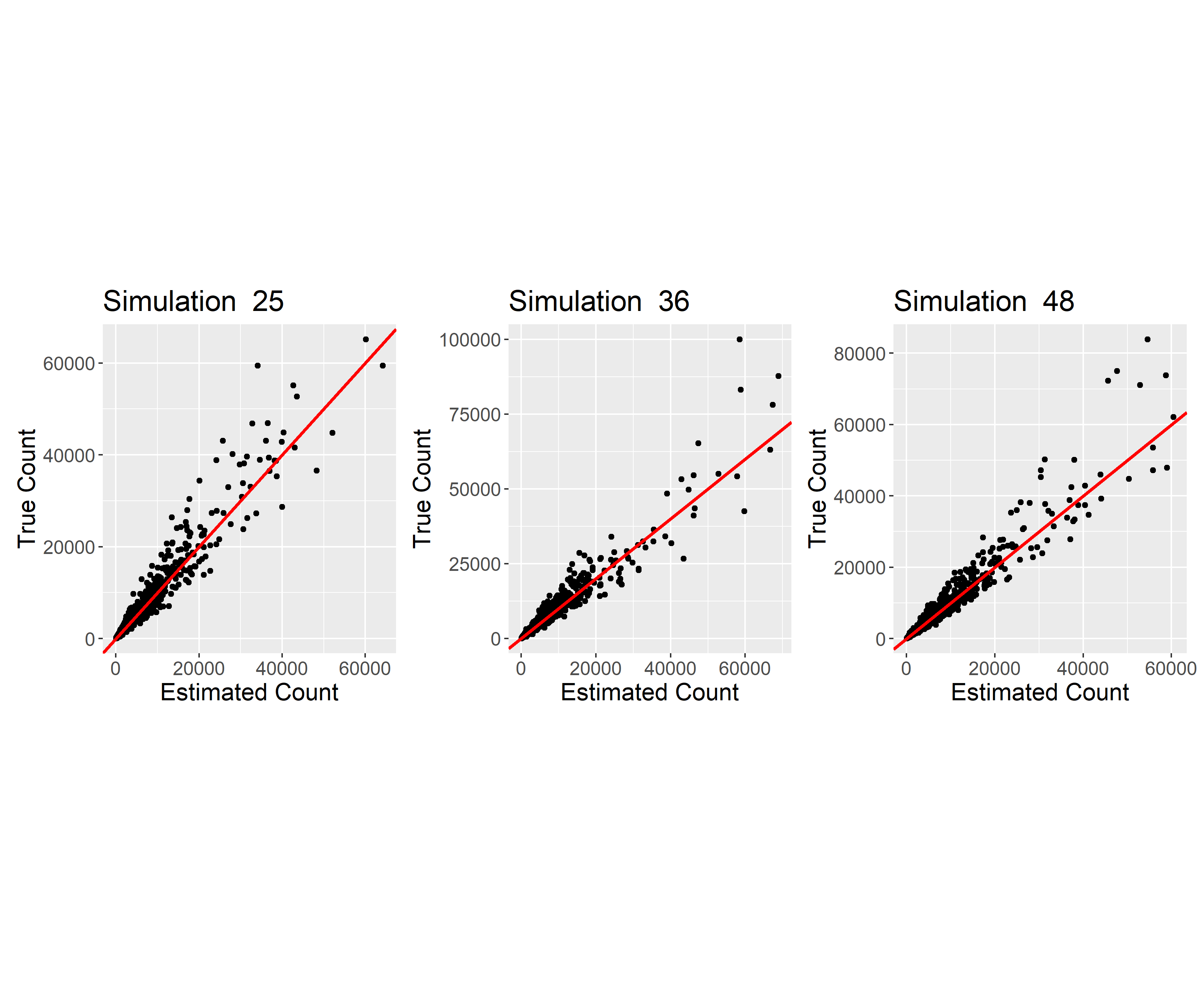
(a) $N_{it}$

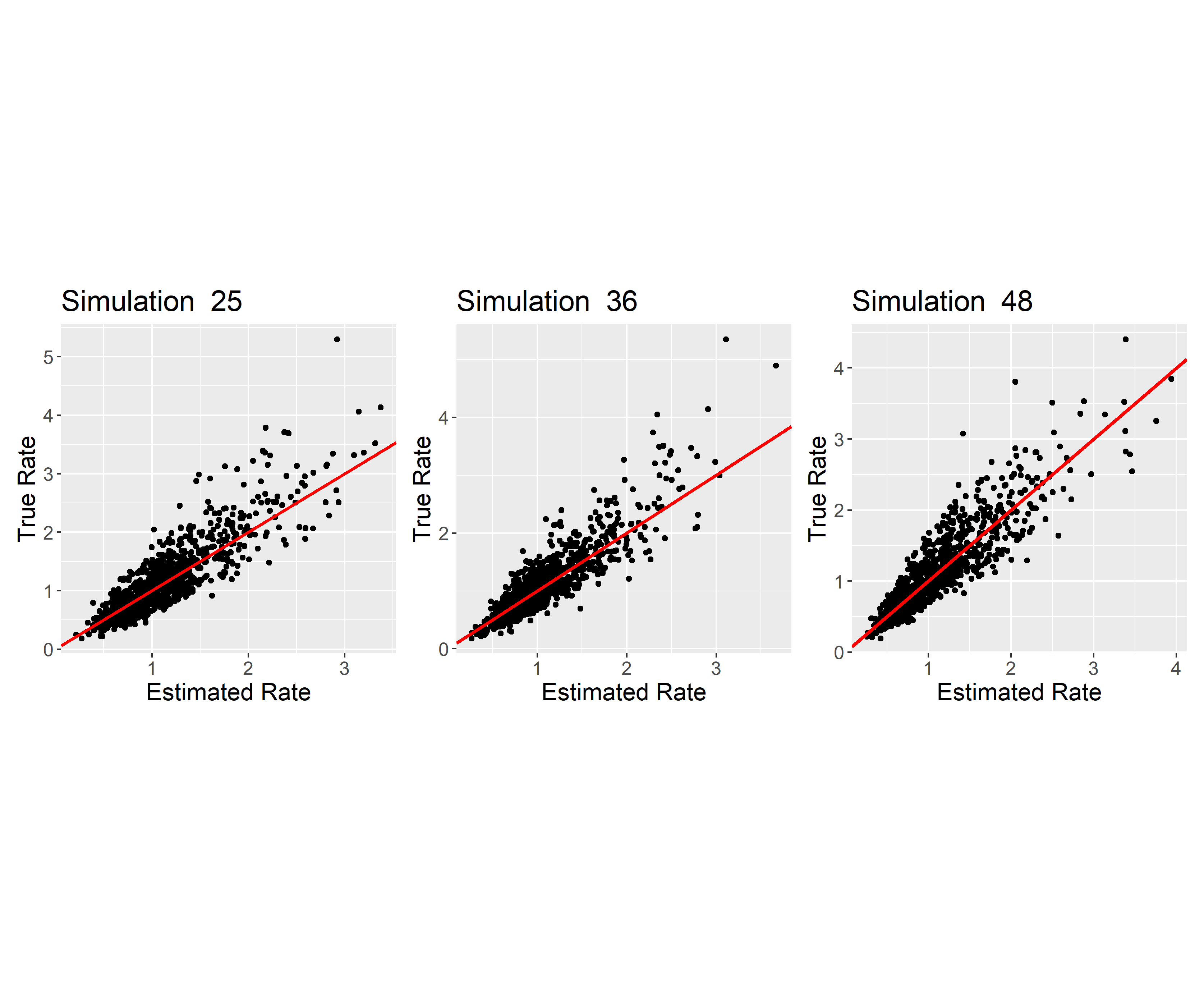
(b) $\lambda_{it}$

Figure 3: Scatterplots from randomly selected simulated data sets showing the estimated and true counts ($N_{it}$) and relative risks ($\lambda_{it}$). Red lines indicate when the estimates equal the truth.

In addition to illustrating that the proposed model has smaller error than competing approaches, we also show that, on average, the proposed model recovers the true parameters of the data generating model. In Supplemental Figure 1, we show that we were able to estimate the intercept parameters $\mu_{t}$ ($\beta^{\mu}_{0}$ and $\beta^{\mu}_{1}$), $\mu_{t}^{(1)}$, and $\mu_{t}^{(2)}$. This suggests that we have adequate information on the range of the detection probabilities to overcome the identifiability issues that are common with abundance models. In addition, we show in Supplemental Figure 2 that we are able to estimate the relative risks, $\lambda_{it}$, quite well. Across the 100 simulated data sets, the average difference between the true and estimated $\lambda_{it}$ is -0.003. Likewise, we show scatterplots of the estimates against the true values for three randomly selected simulated data sets in Supplement Figure 3 and see points clustered around the $y=x$ line, which indicates that the model is generally recovering the truth. Again, this suggests that we are able to recover the true values of the model parameters, suggesting that we have adequate information to inform the model and practically overcome challenges related to identifiability.

In summary, our simulation study showed that our model accurately recovers the latent counts and relative risks and drastically outperforms the baseline model. We have also shown that our model with sparse survey information still outperforms the baseline model, although it is not as good as having yearly survey data. We observe that performance is improved by including multiple observed surveillance outcomes compared to using only a single outcome. Finally, we illustrated that the integration of state-level survey information overcomes limitations of traditional abundance models and adequately informs the estimation of model parameters.

Table 2: A comparison of results from the proposed joint model to the single outcome model. The first two columns show the mean and median coverage probability (CP) across the 100 simulated data sets for $N_{it}$ (proposed/single outcome). The final three columns present the proportion of simulated data sets for which the proposed model results in a smaller error along with the average error across the 100 data sets for each model (proposed/single outcome).

Survey Mean CP Median CP RMSE ($N_{it}$) RMSE ($\lambda_{it}$) Relative MAE ($N_{it}$) Yearly 95%/89% 96%/90% 99/100 100/100 100/100 2598/3559 0.39/0.64 0.16/0.21 Sparse 93%/89% 95%/90% 93/100 94/100 91/100 2890/3665 0.39/0.64 0.17/0.21

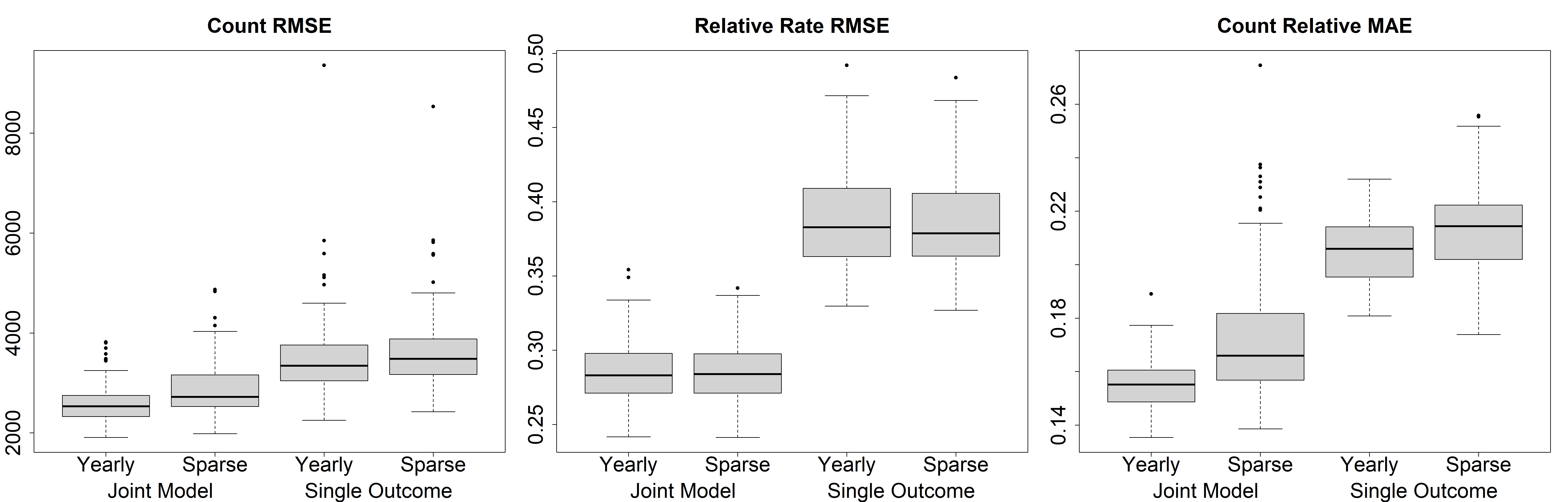
Figure 2: Boxplots of the RMSE for the counts ($N_{it}$) (left) and relative risk ($\lambda_{it}$) (middle) and the relative MAE for the counts ($N_{it}$) (right) for the 100 simulated data sets under the proposed joint model and the single outcome model for cases assuming yearly and sparse survey data.

5 Ohio Prevalence Estimates

In this section, we apply the model defined in Section 2 to estimate the unobserved number of PWMO from 2007-2019 for each of Ohio’s $n=88$ counties. To do so, we utilize $T=13$ years of observed county-level counts of opioid overdose death and treatment admissions and multi-year state-level survey estimates of the prevalence of opioid misuse.

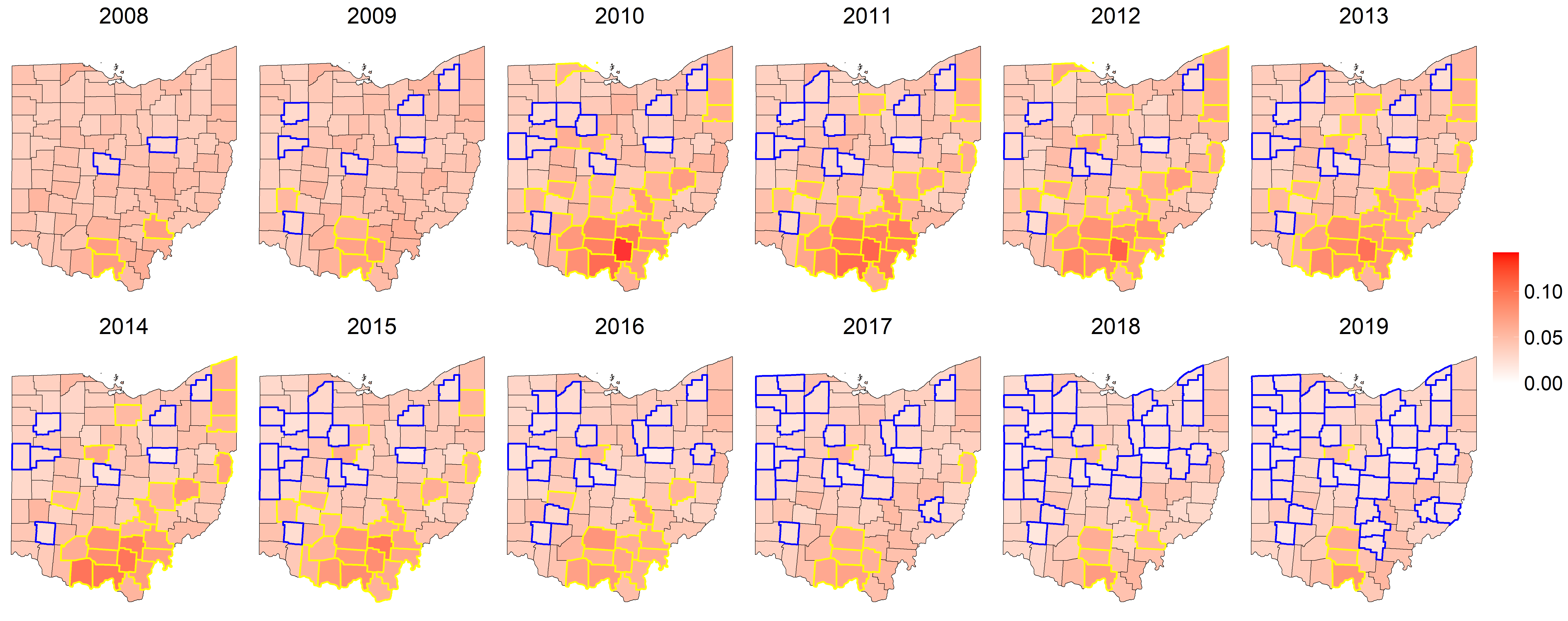
Figure 3: Maps of the estimated prevalence of PWMO, given by $\hat{N}_{it}/P_{it}$. Counties outlined in yellow have 95% credible intervals that are entirely above the baseline estimate, and the counties in blue have credible intervals that are entirely below.

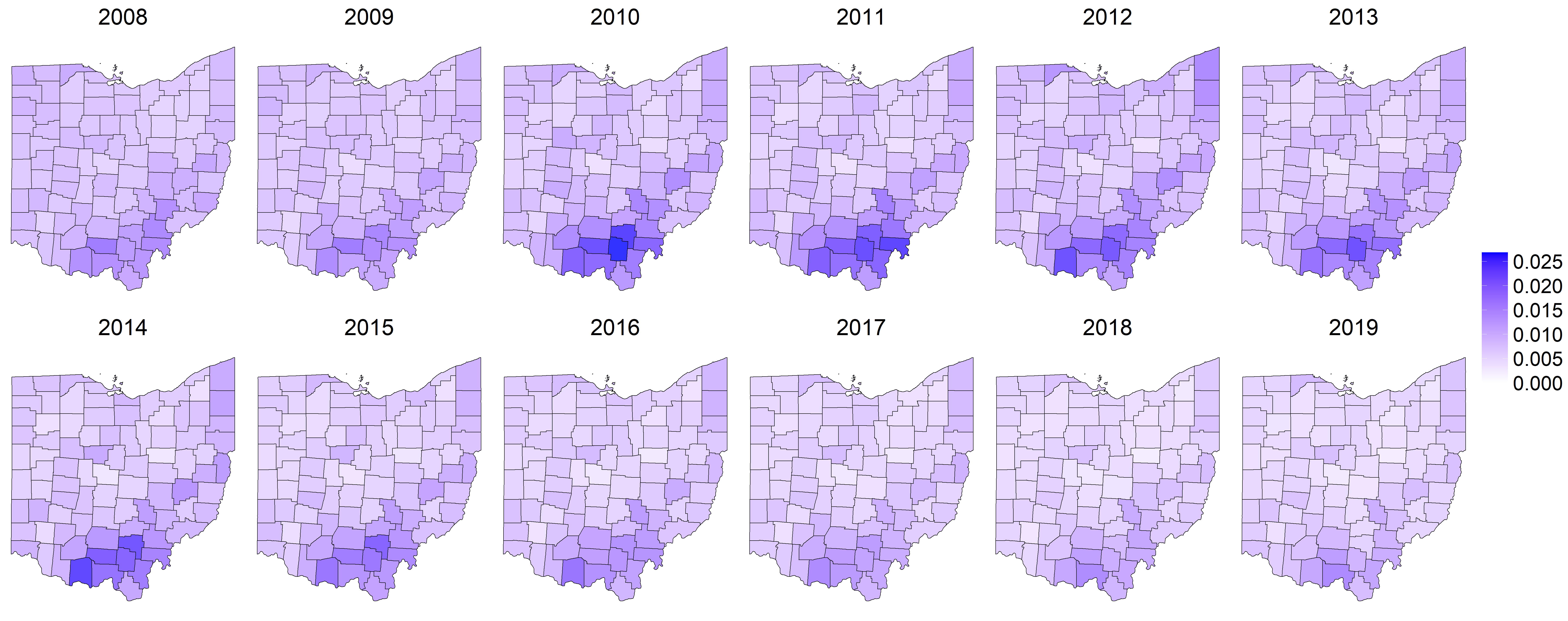
Figure 4: Maps of the standard error of the prevalence of PWMO.

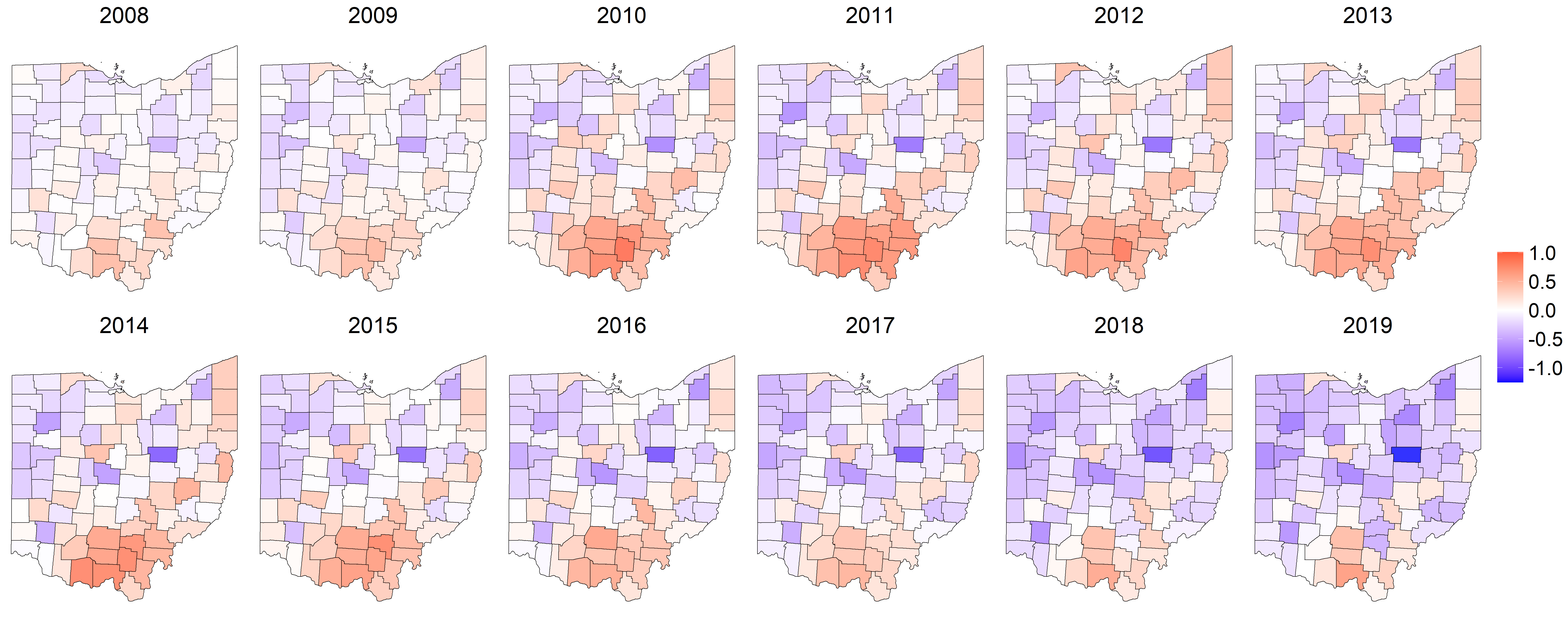
Figure 4: Maps of the estimated relative risk of PWMO, given by $\lambda_{it}$.

Figure 3 maps the posterior mean of the estimate prevalence, $\hat{N}_{it}/P_{it}$, and Figure 4 contains the posterior standard deviation. Maps for the estimated log relative risk, $\log\left(\hat{\lambda}_{it}\right)$, are in the supplementary material. We observe county-level and yearly heterogeneity with prevalence ranging from approximately 0 to nearly 0.13. We observe the highest prevalence in southern Ohio, which is commonly considered the epicenter of the opioid epidemic in Ohio. This map also identifies the counties whose estimated counts of the PWMO are significantly different than would be obtained under the naive baseline estimate that assumes a homogeneous statewide rate, estimated from the survey data. More specifically, the counties outlined in yellow have 95% credible intervals (CI) that are entirely above the baseline estimate, and the counties in blue have CIs that are entirely below.

The statewide average prevalence of misuse parameters were estimated to be $\hat{\beta}_{0}^{\mu}=0.0535$ with 95% CI (0.0516 to 0.0557) and $\hat{\beta}_{1}^{\mu}=-0.0006$ with 95% CI (-0.0009 to -0.0004). Table 3 contains the corresponding information for the prevalence of misuse regression coefficients. We observe a 5% increase in prevalence per standard deviation increase in unemployment and high school education, a roughly 10% increase per standard deviation increase in poverty and food stamps, and a 24% increase per standard deviation increase in prescribing rate.

Table 3: Posterior mean and 95% credible intervals of prevalence ratios per 1 standard deviation change in each covariate for prevalence of PWMO.

Variable Estimate 95% CI Poverty 1.10 (1.08, 1.13) Unemployment 1.05 (1.01, 1.08) High School 1.05 (1.02, 1.08) Food Stamps 1.11 (1.08, 1.15) Prescribing Rate 1.24 (1.19, 1.29)

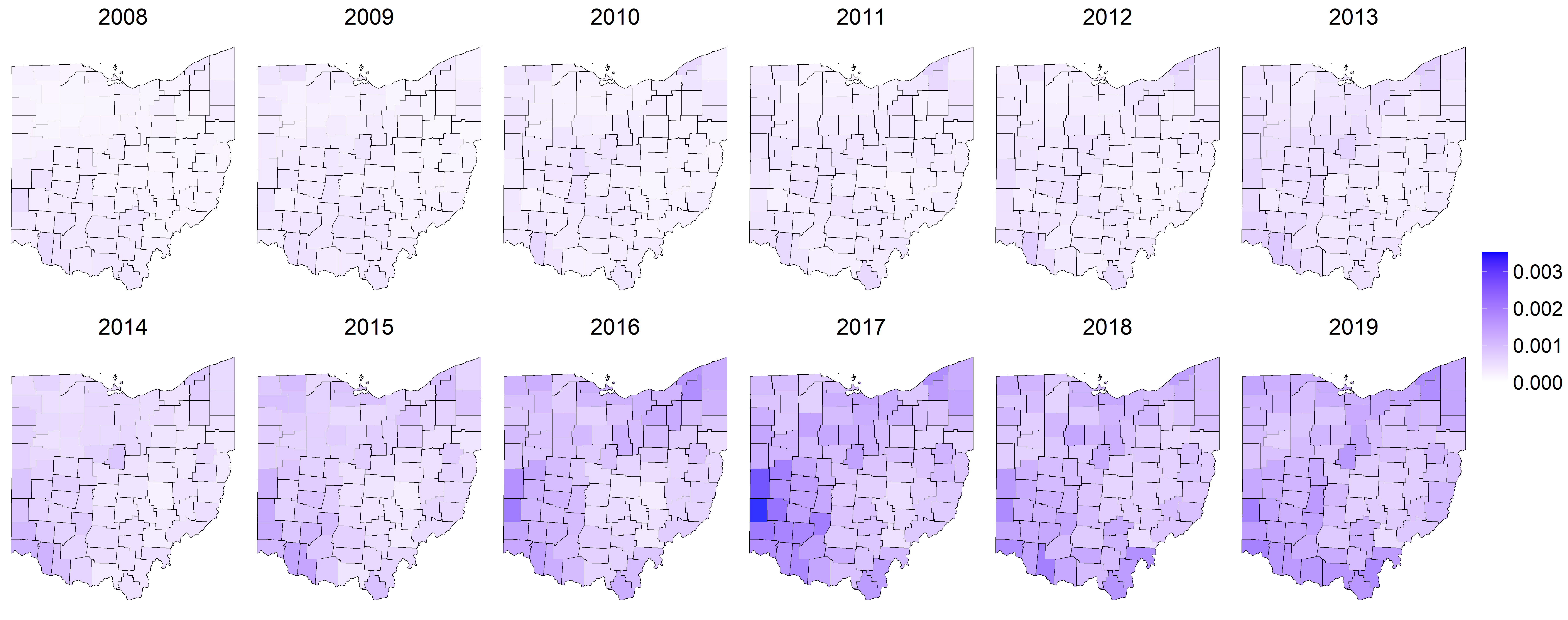
Figure 5: Maps of the posterior standard deviation of the death rate, $p^{(D)}_{it}$.

Figure 5 is a map of the estimated death rate among PWMO, $\hat{p}^{(D)}_{it}$. A map of the standard errors is in the supplementary material. In the earlier years, we see very low death rates with a large degree of spatial heterogeneity. Starting around 2012, we see increases in the death rate for the southwestern Ohio region corresponding to the Cincinnati, Ohio area, followed by increasing rates in the northeastern Cleveland, Ohio region. This is likely due to the influx of fentanyl in these regions during this time period (Daniulaityte et al., 2017; Pardo et al., 2019). Table 4 shows the posterior means and 95% credible intervals for the odds ratios for the death rate. We estimate that the odds of death are 19% higher in metropolitan statistical areas compared to non-metropolitan areas.

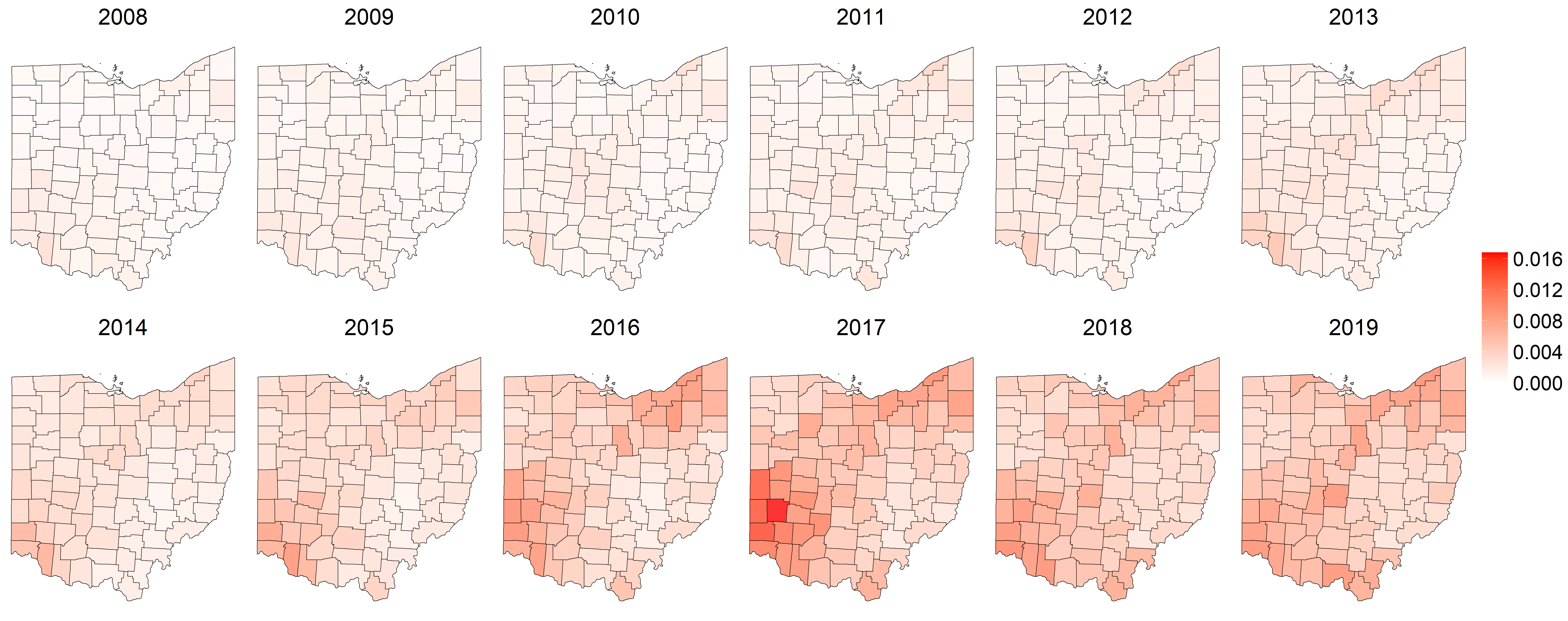
Figure 5: Maps of the estimated death rate among PWMO, $\hat{p}^{(D)}_{it}$.

Table 4: Posterior means and 95% credible intervals for the odds ratios corresponding to the covariates in the models for death rate and treatment rate among PWMO.

Variable Estimate CI Death Rate Interstates 1.04 (0.96, 1.14) HIDTA 1.07 (0.97, 1.17) MSA 1.19 (1.08, 1.30) Treatment Rate HPSA 0.91 (0.85, 0.98) MU 1.01 (0.93, 1.09)

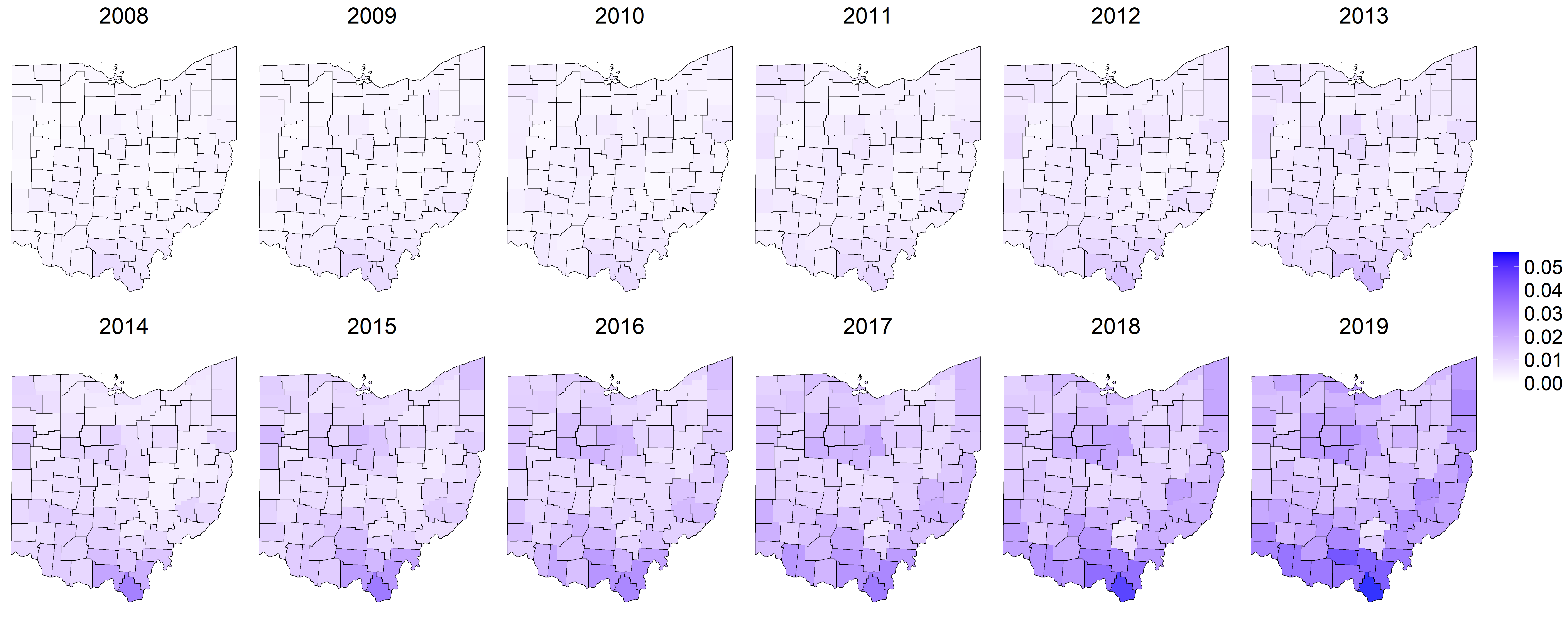
Figure 6: Maps of the posterior standard deviation of the treatment rate, $p^{(T)}_{it}$.

Similarly, Figure 6 maps the estimated treatment rates among PWMO, $\hat{p}^{(T)}_{it}$. A map of the standard errors is in the supplementary material. We generally see an increasing treatment rate over time, with the largest rates in southern Ohio which is known to have received a large number of resources towards treatment of opioid misuse (Governor’s Cabinet Opiate Action Team, 2012). Table 4 shows the posterior means and 95% credible intervals for the treatment rate odds ratios. We estimate that the odds of treatment are 9% less in health professional shortage areas compared to non-shortage areas.

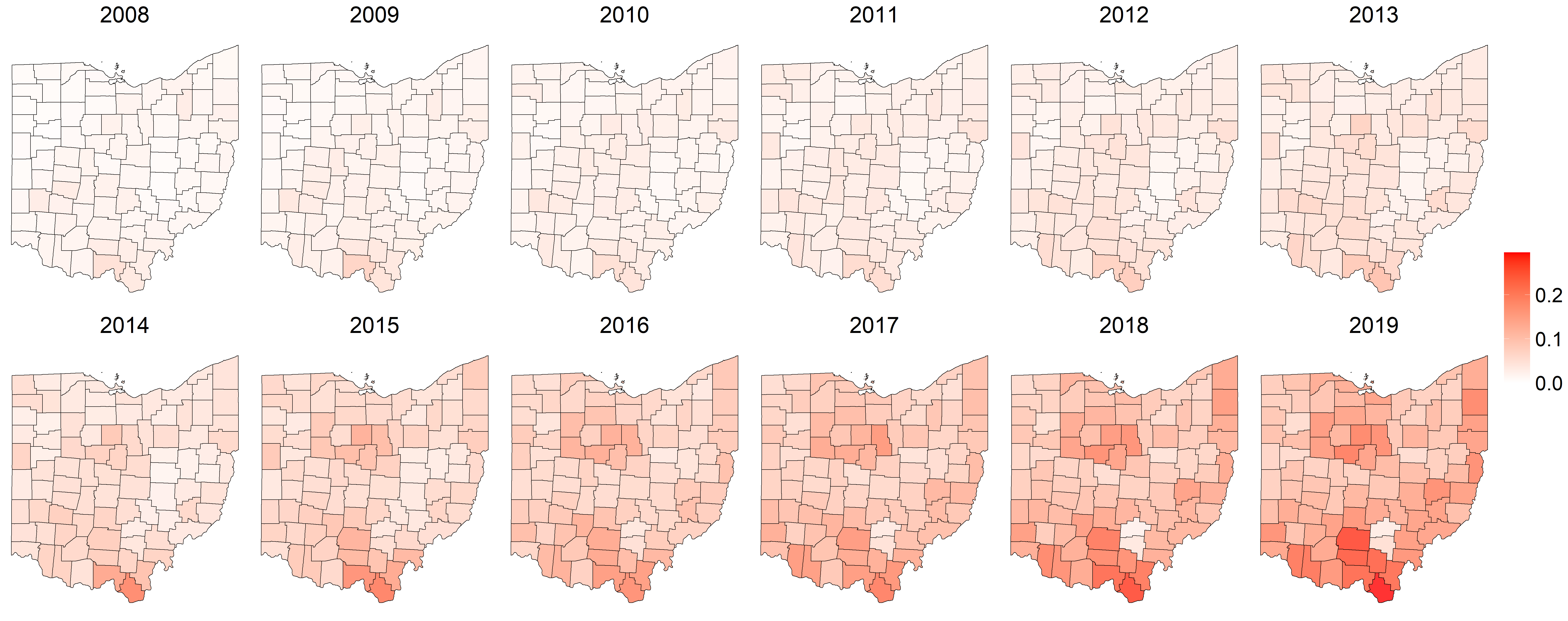
Figure 6: Maps of the estimated treatment rates $\hat{p}^{(T)}_{it}$ for each county from 2007 to 2018.

Figure 7 plots the time-varying intercepts for death and treatment rates, $\mu_{t}^{(D)}$ and $\mu_{t}^{(T)}$. Recall the covariates included for both logistic regression models are indicator variables, so the intercepts for death are interpreted as the yearly average death rates (on the logit scale) among counties without interstates that are neither high impact drug trafficking areas nor metropolitan statistical areas. We generally observe an increasing trend, with a sharp increase beginning in 2012. The years following 2012 correspond to the time in which fentanyl began to infiltrate the state, resulting in a drastic increase in overdose deaths (Pardo et al., 2019). The estimates of $\mu_{t}^{(T)}$ represent the yearly average treatment rates (on the logit scale) among counties that are neither health professional shortage areas nor medically underserved areas. We see a generally increasing trend with slight shifts observed in 2010 and also in 2014. We note that these time periods align with the passing of state legislation expanding access to treatment (Governor’s Cabinet Opiate Action Team, 2012) and also with Medicaid expansion which occurred in Ohio in 2014.

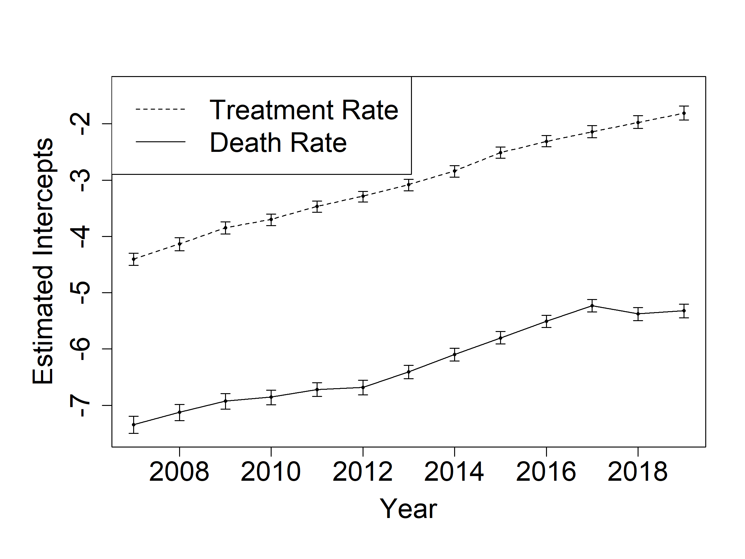
Figure 7: Plot of the time-varying intercepts for treatment and death

6 Discussion

In this paper, we developed an approach for estimating the county-level prevalence of PWMO using indirect information from observed, aggregate surveillance outcomes synthesized within an abundance model framework. By integrating state-level external information, we showed that our model can identify the intercepts at both the level of the latent counts and for the observed surveillance data. We also show that this approach is superior to assuming homogeneity across counties and to using a single surveillance outcome. By coherently leveraging joint information across data sources, we were able to recover model-based estimates of the latent counts of interest.

We applied our framework to estimate annual county-level counts and prevalence of PWMO in Ohio over a 13 year period. By doing so, we were able to estimate the prevalence of PWMO, which is extremely relevant for public health policy and until this point, estimates did not exist at the county-level across the state. In addition, we estimated death and treatment rates within the population of PWMO. This is in contrast to typical epidemiological analyses that define the population at risk as the whole population rather than just the PWMO. Therefore, the estimates of these rates are more relevant for describing trends in PWMO and informing the targeting of resources and harm reduction interventions. These estimates can also be used to fill data gaps by informing key model parameters in simulation models developed to inform policy choices (Jalali et al., 2020). We also described associations with covariates at each level of the model.

Our work forms a foundation for this line of research as there are additional methodological challenges to address. For instance, the primary goal of our simulation study was to establish the model’s ability to accurately estimate the latent counts and prevalence of PWMO. We have not thoroughly assessed the conditions required to accurately estimate covariate effects. This issue of identifying covariate effects for both observed and latent processes has been studied under various settings (e.g. Lele et al. (2012); Hepler et al. (2018); Stoner et al. (2019)), but the results of those papers may not hold since we integrate multiple observed variables at the desired spatial support with additional information at the state level. A future research question is to investigate how well and under what conditions our model can estimate covariate effects. Additional avenues for future research include studying advantages and disadvantages of including more outcome variables and also utilizing our model to evaluate policy and optimize resource allocation.

Our analysis has several limitations. First, we assume the surveillance outcomes are observed without error, but there is potential for misclassification, particularly of overdose deaths (Slavova et al., 2015). However, Ohio is considered to have excellent reporting of overdose deaths (Scholl et al., 2019). We also use survey estimates to inform the intercepts which are potentially underreported. While the model can flexibly adjust estimates around the parameters informed by the survey, future work will formally explore sensitivity to bias in the survey estimates. In addition, the language of the survey question addressing opioid misuse was changed in 2015 which may have impacted responses. We also assume that all individuals counted as a treatment admission or an overdose death belong to the population of PWMO. While this is a reasonable assumption, it is unlikely to be universally true, particularly as fentanyl is unknowingly added to other substances (Mars et al., 2019; Townsend et al., 2021). In addition, all analyses are aggregate and should be interpreted at the appropriate level to avoid the ecological fallacy (Pianntadosi et al., 1988).

In conclusion, we have a developed a model within the abundance model framework to estimate the size of hidden populations using observed data that provide indirect information. Through synthesis of multiple sources of data, we are able to generate model-based estimates of hidden quantities that are critical for informing public health policy and the allocation of resources. We believe this is a promising framework for addressing questions about hidden epidemiological populations and can provide a foundation for future research.

Supplemental Material

Table 1: Estimates of the average statewide prevalence of misuse
                                                                                                                                   over the given time frame along with standard errors of the estimates.

Years Estimate Standard Error 2003 - 2006 0.05 0.0025 2007 - 2010 0.055 0.0026 2011 - 2014 0.052 0.0024 2015 - 2016 0.047 0.0041 2016 - 2017 0.051 0.0037 2017 - 2018 0.041 0.0033 2018 - 2019 0.043 0.0043

References

- Banerjee et al. (2004) Banerjee, S., Carlin, B. P. and Gelfand, A. E. (2004) Hierarchical modeling and analysis for spatial data. Boca Raton, Fla.: Chapman & Hall/CRC.
- Bao et al. (2015) Bao, L., Raftery, A. and Reddy, A. (2015) Estimating the sizes of populations at risk of hiv infection from multiple data sources using a bayesian hierarchical model. Statistics and Its Interface, 8, 125–136.
- Barocas et al. (2018) Barocas, J. A., White, L. F., Wang, J., Walley, A. Y., LaRochelle, M. R., Bernson, D., Land, T., Morgan, J. R., Samet, J. H. and Linas, B. P. (2018) Estimated prevalence of opioid use disorder in Massachusetts, 2011–2015: A capture–recapture analysis. American Journal of Public Health, 108, 1675–1681. PMID: 30359112.
- Berliner (1996) Berliner, L. (1996) Hierarchical Bayesian time series models. In Maximum Entropy and Bayesian Methods (eds. K. Hanson and R. Silver), 15–22. Dordrecht: Kluwer Academic Publishers.
- Besag (1974) Besag, J. (1974) Spatial interaction and the statistical analysis of lattice systems. Journal of the Royal Statistical Society. Series B (Methodological), 36, 192–236.
- Besbeas et al. (2002) Besbeas, P., Freeman, S., Mordan, B. and Catchpole, E. (2002) Integrating mark-recapture-recovert and census data to estimate animal abundance and demographic parameters. Biometrics, 58, 540–547.
- Bradley et al. (2015) Bradley, J. R., Wikle, C. K. and Holan, S. H. (2015) Spatio-temporal change of support with application to American Community Survey multi-year period estimates. Stat, 4, 255–270.
- Burke and Buchanich (2018) Burke, D. and Buchanich, J. (2018) Drug overdoses in pennsylvania: Measuring, tracking, and forecasting the epidemic. Commonwealth: A Journal of Pennsylvania Politics and Policy, 20, 23–37.
- CDC (2021) CDC, N. C. f. H. S. (2021) Drug overdose deaths in the U.S. top 100,000 annually. URL: https://www.cdc.gov/nchs/pressroom/nchs_press_releases/2021/20211117.htm.
- Cole (2020) Cole, D. J. (2020) Parameter Redundancy and Identifiability. Boca Raton: CRC Press.
- Crawford et al. (2018) Crawford, F. W., Wu, J. and Heimer, R. (2018) Hidden population size estimation from respondent-driven sampling: A network approach. Journal of the American Statistical Association, 113, 755–766.
- Cressie et al. (2005) Cressie, N., Perrin, O. and Thomas-Agnan, C. (2005) Likelihood-based estimation for Gaussian mrfs. Statistical Methodology, 2, 1–16.
- Cressie and Wikle (2011) Cressie, N. A. C. and Wikle, C. K. (2011) Statistics for spatio-temporal data. Hoboken, N.J.: Wiley.
- Daniulaityte et al. (2017) Daniulaityte, R., Juhascik, M. P., Strayer, K. E., Sizemore, I. E., Harshbarger, K. E., Antonides, H. M. and Carlson, R. R. (2017) Overdose deaths related to fentanyl and its analogs - Ohio, January-February 2017. MMWR. Morbidity and mortality weekly report, 66, 904–908.
- de Valpine et al. (2017) de Valpine, P., Turek, D., Paciorek, C., Anderson-Bergman, C., Temple Lang, D. and Bodik, R. (2017) Programming with models: writing statistical algorithms for general model structures with NIMBLE. Journal of Computational and Graphical Statistics, 26, 403–417.
- Division of Unintentional Injury Prevention (2021) Division of Unintentional Injury Prevention (2021) Drug overdose deaths. Internet. https://www.cdc.gov/drugoverdose/deaths/index.html.
- Drug Enforcement Agency (2016) Drug Enforcement Agency (2016) 2016 national drug threat assessment. Internet. https://www.dea.gov/resource-center/2016\%20NDTA\%20Summary.pdf.
- Famoye and Wang (2004) Famoye, F. and Wang, W. (2004) Censored generalized poisson regression model. Computational Statistics and Data Analysis, 46, 547–560.
- Governor’s Cabinet Opiate Action Team (2012) Governor’s Cabinet Opiate Action Team (2012) Attacking Ohio’s opiate epidemic. Online; accessed 6-September-2017. https://mha.ohio.gov/Researchers-and-Media/Combating-the-Opioid-Crisis.
- Handcock et al. (2014) Handcock, M. S., Gile, K. J. and Mar, C. M. (2014) Estimating hidden population size using respondent-driven sampling data. Electronic Journal of Statistics, 8, 1491–1521.
- Hepler et al. (2018) Hepler, S., Erhardt, R. and Anderson, T. (2018) Identifying drivers of spatial variation in occupancy with limited replication camera trap data. Ecology, 99, 2152–2158.
- Jalali et al. (2020) Jalali, M. S., Ewing, E., Bannister, C. B., Glos, L., Eggers, S., Lim, T. Y., Stringfellow, E., Stafford, C. A., Pacula, R. L., Jalal, H. and Kazemi-Tabriz, R. (2020) Data needs in opioid systems modeling: Challenges and future directions. American Journal of Preventive Medicine. URL: http://www.sciencedirect.com/science/article/pii/S0749379720303998.
- Jones et al. (2016) Jones, H. E., Welton, N. J., Ades, A. E., Pierce, M. and Davies, W. (2016) Problem drug use prevalence estimation revisited: heterogeneity in capture-recapture and the role of external evidence. Addiction, 111, 438–447.
- Kery and Royle (2010) Kery, M. and Royle, A. (2010) Hierarchical modelling and estimation of abundance and population trends in metapopulation designs. Journal of Animal Ecology, 79, 453–461.
- Knape et al. (2015) Knape, J., Korner-Nievergelt, F. and Yoccoz, N. (2015) Estimates from non-replicated population surveys rely on critical assumptions. Methods in Ecology and Evolution, 6, 298–306.
- Lele et al. (2012) Lele, S., Moreno, M. and Bayne, E. (2012) Dealing with detection error in site occupancy surveys: what can we do with a single survey? Journal of Plant Ecology, 5, 22–31.
- Lerner and Fauci (2019) Lerner, A. M. and Fauci, A. S. (2019) Opioid Injection in Rural Areas of the United States: A Potential Obstacle to Ending the HIV Epidemic. JAMA, 322, 1041–1042.
- Mars et al. (2019) Mars, S. G., Rosenblum, D. and Ciccarone, D. (2019) Illicit fentanyls in the opioid street market: desired or imposed? Addiction, 114, 774–780.
- Min et al. (2020) Min, J. E., Pearce, L. A., Homayra, F., Dale, L. M., Barocas, J. A., Irvine, M. A., Slaunwhite, A. K., McGowan, G., Torban, M. and Nosyk, B. (2020) Estimates of opioid use disorder prevalence from a regression-based multi-sample stratified capture-recapture analysis. Drug and Alcohol Dependence, 217, 108337.
- Neath and Samaniego (1997) Neath, A. and Samaniego, F. (1997) On the efficacy of Bayesian inference for nonidentifiable models. The American Statistician, 51, 225–232.
- Office of National Drug Control Policy Executive, Office of the President of the United States (2011) Office of National Drug Control Policy Executive, Office of the President of the United States (2011) Epidemic: responding to America’s prescription drug abuse crisis. Internet. https://www.hsdl.org/?view&did=4609.
- Ohio Public Health Data Warehouse (2020) Ohio Public Health Data Warehouse (2020) Ohio resident mortality data. http://publicapps.odh.ohio.gov/EDW/DataCatalog. Accessed February 2, 2020.
- Paciorek (2009) Paciorek, C. (2009) Technical vignette 5: Understanding intrinsic Gaussian Markov random field spatial models, including intrinsic conditional autoregressive models. Tech. rep., Department of Statistics, University of California, Berkeley and Department of Biostatistics, Harvard School of Public Health.
- Palamar et al. (2016) Palamar, J. J., Shearston, J. A. and Cleland, C. M. (2016) Discordant reporting of nonmedical opioid use in a nationally representative sample of US high school seniors. The American Journal of Drug and Alcohol Abuse, 42, 530–538.
- Pardo et al. (2019) Pardo, B., Taylor, J., Caulkins, J. P., Kilmer, B., Reuter, P. and Stein, B. D. (2019) The Future of Fentanyl and Other Synthetic Opioids. Santa Monica, CA: RAND Corporation.
- Pianntadosi et al. (1988) Pianntadosi, S., Byar, D. P. and Green, S. B. (1988) The ecological fallacy. American Journal of Epidemiology, 127, 893–904.
- Rembert et al. (2017) Rembert, M., Betz, M., Feng, B. and Partridge, M. (2017) Taking measure of Ohio’s opioid crisis. https://aede.osu.edu/sites/aede/files/publication_files/Swank%20-%20Taking%20Measure%20of%20Ohios%20Opioid%20Crisis.pdf.
- Royle (2004) Royle, J. A. (2004) N-mixture models for estimating population size from spatially replicated counts. Biometrics, 60, 108–115.
- Rudd et al. (2016) Rudd, R., Seth, P., David, F. and Scholl, L. (2016) Increases in drug and opioid-involved overdose deaths - United States, 2010-2015. MMWR Morb Mortal Wkly Rep.
- SAMHSA, Center for Behavioral Health Statistics and Quality (2003-2005, 2006-2008, 2009-2010, 2011-2014) SAMHSA, Center for Behavioral Health Statistics and Quality (2003-2005, 2006-2008, 2009-2010, 2011-2014) National survey on drug use and health. http://www.samhsa.gov/.
- SAMHSA, Center for Behavioral Health Statistics and Quality (2015-2016, 2016-2017, 2017-2018, 2018-2019) — (2015-2016, 2016-2017, 2017-2018, 2018-2019) National survey on drug use and health, 2-year RDAS. http://www.samhsa.gov/.
- Schaub and Abadi (2011) Schaub, M. and Abadi, F. (2011) Integrated population models: A novel analysis framework for deeper insights into population dynamics. Journal of Ornithology, 152, 227–237.
- Scholl et al. (2019) Scholl, L., Seth, P., Kariisa, M., Wilson, N. and Baldwin, G. (2019) Drug and opioid-involved overdose deaths - united states, 2013-2017. MMWR, 67, 1419–1427.
- Schuler et al. (2020) Schuler, M. S., Griffin, B. A., Cerdá, M., McGinty, E. E. and Stuart, E. A. (2020) Methodological challenges and proposed solutions for evaluating opioid policy effectiveness. Health Services and Outcomes Research Methodology. In press.
- Slavova et al. (2015) Slavova, S., O’Brien, D. B., Creppage, K., Dao, D., Fondario, A., Haile, E., Hume, B., Largo, T. W., Nguyen, C., Sabel, J. C., Wright, D. and Members of the Council of State and Territorial Epidemiologists Overdose Subcommittee (2015) Drug overdose deaths: Let’s get specific. Public health reports, 130.
- Sólymos et al. (2012) Sólymos, P., Lele, S. and Bayne, E. (2012) Conditional likelihood approach for analyzing single visit abundance survey data in the presence of zero inflation and detection error. Environmetrics, 23, 197–205.
- Stoner et al. (2019) Stoner, O., Economou, T. and da Silva, G. D. M. (2019) A hierarchical framework for correcting under-reporting in count data. Journal of the American Statistical Association, 0, 1–17.
- Townsend et al. (2021) Townsend, T., Kline, D., Rivera-Aguirre, A., Bunting, A., Mauro, P., Marshall, B., Martins, S. and Cerdá, M. (2021) Racial/ethnic and geographic trends in combined stimulant/opioid overdoses, 2007-2019. American Journal of Epidemiology. In press.
- Zibbell et al. (2015) Zibbell, J., Igbal, K., Patel, R., Suryaprasad, A., Sanders, K., Moore-Moravian, L., Serrecchia, J., Blankenship, S., Ward, J., Holtzman, D. and Centers for Disease Control and Prevention (2015) Increases in hepatitis c virus infection related to injection drug use among persons aged 30 years - kentucky, tennessee, virginia, and west virginia, 2006-2012. MMWR, 64, 453–458.