Stellar Rotation in the Gaia Era: Revised Open Clusters Sequences

Abstract

The period versus mass diagrams (i.e., rotational sequences) of open clusters provide crucial constraints for angular momentum evolution studies. However, their memberships are often heavily contaminated by field stars, which could potentially bias the interpretations. In this paper, we use data from Gaia DR2 to re-assess the memberships of seven open clusters with ground- and space-based rotational data, and present an updated view of stellar rotation as a function of mass and age. We use the Gaia astrometry to identify the cluster members in phase-space, and the photometry to derive revised ages and place the stars on a consistent mass scale. Applying our membership analysis to the rotational sequences reveals that: 1) the contamination in clusters observed from the ground can reach up to $\sim 35\%$; 2) the overall fraction of rotational outliers decreases substantially when the field contaminants are removed, but some outliers persist; 3) there is a sharp upper edge in the rotation periods at young ages; 4) at young ages, stars in the $1.0\textendash 0.6M_{\odot}$ range inhabit a global maximum of rotation periods, potentially providing an optimal window for habitable planets. Additionally, we see clear evidence for a strongly mass-dependent spin-down process. In the regime where rapid rotators are leaving the saturated domain, the rotational distributions broaden (in contradiction with popular models), which we interpret as evidence that the torque must be lower for rapid rotators than for intermediate ones. The cleaned rotational sequences from ground-based observations can be as constraining as those obtained from space.

1 Introduction

Together with mass and metallicity, rotation is one of the defining properties of stars. Stellar rotation is strongly mass-dependent (Kraft, 1967a; García et al., 2014), and while stars with radiative envelopes ($M\gtrsim 1.4M_{\odot}$) live their lives as rapid rotators, stars with convective envelopes spin down as they age (Skumanich, 1972). The overall framework of the rotational evolution of low mass stars is that they are born with a range of rotation rates ($\sim 1\textendash 10$ days; Herbst et al. 2002) and star-disk coupling timescales (from $<1$ and up to $\sim 10$ Myr; Williams & Cieza 2011), and once they arrive onto the zero-age main-sequence (ZAMS), they experience a decrease in their rotational velocities due to angular momentum losses caused by magnetized winds (Parker, 1958; Schatzman, 1962; Weber & Davis, 1967; Kawaler, 1988; Pinsonneault et al., 1989).

For lower main-sequence stars, the observable stellar properties do not appreciably change with time, which makes the determination of ages of individual stars challenging (Soderblom, 2010). In this regard, the empirical spin-down of low mass stars offers a valuable age diagnostic, and this idea is known as gyrochronology (Barnes, 2003, 2007; Mamajek & Hillenbrand, 2008).

If properly validated, gyrochronology can provide valuable age information for Galactic and stellar population studies (McQuillan et al., 2013, 2014; Davenport, 2017; Davenport & Covey, 2018; van Saders et al., 2019), as well as for the characterization of exoplanet hosts (e.g., Gallet & Delorme 2019; Gallet 2020; Zhou et al. 2021; Carmichael et al. 2021; David et al. 2021). Moreover, although stellar evolution theory is successful in predicting numerous properties of stars, this is not the case for the evolution of angular momentum and its related physical processes (e.g., transport in stellar interiors, birth conditions, magnetic braking). Consequently, stellar models that incorporate it need to be calibrated with empirical observations (e.g., Gossage et al. 2021).

All of the above add to a compelling need for gyrochronology to be examined and tested. For old ages ($\gtrsim$ few Gyr), these efforts have used field stars (Irwin et al., 2011; Angus et al., 2015; Newton et al., 2016; van Saders et al., 2016; Lorenzo-Oliveira et al., 2019) and wide separation binaries (Chanamé & Ramírez, 2012; Janes, 2017; Godoy-Rivera & Chanamé, 2018; Otani et al., 2021). For young ages ($\lesssim 1$ Gyr), the calibrations have been based on the empirical rotational sequences (i.e., period versus mass or temperature diagrams) of star-forming regions, associations, and open clusters (Denissenkov et al., 2010; Gallet & Bouvier, 2013, 2015; Angus et al., 2019; de Freitas, 2021).

With the advent of space-based missions, the field of stellar rotation is entering a new era. The unparalleled astrometry from the Gaia mission (Gaia Collaboration et al., 2018a) has already allowed new gyrochronology inspections to be carried out (e.g., Curtis et al. 2019b; Angus et al. 2020). In addition to this, results obtained from the observations by the Kepler and K2 missions (Borucki et al., 2010; Howell et al., 2014) have showed striking trends at various ages. These include strongly mass-dependent rotation rates in populations younger than 10 Myr (Somers et al., 2017; Rebull et al., 2018, 2020), unusual spin-down behavior in $\sim 1\textendash 3$ Gyr-old clusters (Curtis et al. 2019a, 2020; Gruner & Barnes 2020; see also Agüeros et al. 2018), and anomalously rapid rotation in $\gtrsim 5$ Gyr-old field stars (van Saders et al., 2016; Hall et al., 2021).

The strengths of space data, namely unparalleled time coverage and photometric precision, have indeed provided exquisite data in selected regimes. However, for many interesting clusters, a combination of crowded fields, faint sources, and long rotation periods, make obtaining data from space surveys impractical. By contrast, ground-based surveys can measure precise and accurate rotation periods for even faint sources, because star spot modulation induces relatively large photometric signals. The native seeing even from average sites is also far better than the 4″ pixels of Kepler and K2, or the 21″ pixels of the Transiting Exoplanet Survey Satellite (TESS; Ricker et al. 2015). As a result, ground-based surveys are still fundamental for studies of stellar rotation.

In this context, although star clusters have played a crucial role in our understanding of angular momentum evolution, a thorough decontamination of their rotational sequences is currently lacking. For the systems that have been observed from the ground, the field contamination in their sequences is expected to go from $\sim 20\%$ (e.g., Hartman et al. 2009a) and reach up to $\sim 40\textendash 60\%$ (e.g., Irwin et al. 2007a, 2008, 2009). For the systems observed from space, a lower contamination rate may be expected due to more careful target selections, but given their importance as rotational benchmarks, detailed astrometric analysis are certainly needed. Furthermore, it has been common in the literature to assume that rotational outliers of cluster sequences correspond to field contaminants. We are now in a position to test this assumption.

Ultimately, the unknown extent to which contamination is a problem, and what effect this could have on the patterns of the rotational sequences, make the revision of their memberships an imperative task. This is something the unprecedented space-based data from Gaia is particularly well-suited for. With this, the goal of this paper is to use the high-precision Gaia astrometry to clean the rotational sequences of a sample of open clusters (observed from the ground and space), with the prospects of providing revised gyrochronology calibrators, and an updated view of stellar rotation as a function of mass and age.

This paper is structured as follows. In §2 we present the sample of star clusters with rotation period measurements we study. In §3 we present our method for identifying likely cluster members using the Gaia astrometry. In §4 we revise the properties of the clusters we study, and calculate stellar masses and temperatures for their members. In §5 we show the effects that the membership analysis has on the rotational sequences. In §6 we discuss our findings and present an updated view of stellar rotation. We conclude in §7.

2 Sample Selection and Rotation Period Data

We compile a list of open clusters that satisfy four conditions: 1) they hold high scientific interest for constraining the processes that govern stellar rotation; 2) they have rotation period information, derived uniformly within each cluster, for $\sim$ hundreds of candidate members; 3) they have reliable Gaia data that allows us to accurately model them astrometrically; 4) they potentially have enough non member contamination that a careful membership analysis to clean their rotational sequences would have significant impact. The rotation periods we use come from both ground- and space-based optical photometric monitoring. Due to the target selections of the original rotation period references, the membership contamination is expected to be higher for the clusters observed from the ground than for those observed from space (see the clusters’ descriptions below).

We limit our selection to open clusters but do not include star-forming regions and associations, which require a more complex treatment of membership (e.g., Gagné & Faherty 2018; Galli et al. 2018; Kuhn et al. 2019). We also exclude systems that are either too close or too distant for a reliable membership analysis, or that have poor Gaia data, or systems with smaller or heterogeneous rotation samples. We discuss the systems with available rotational data sets that we did not analyze in Appendix A.

Table 1 lists the seven open clusters we study, together with the number of stars in each of them with period measurements. Table 1 also reports their literature ages as compiled by Gallet & Bouvier (2015) (see their Table 1 for the specific references), but we highlight that for our analysis we perform an independent derivation of revised cluster properties using Gaia data and recent spectroscopic results (see §4). We now describe the seven clusters in our sample.

Table 1: List of the seven open clusters we study.

Name	Literature Age (pre Gaia)	N${}_{\star\text{,Period}}$
-	[Myr]	-
NGC 2547	35	176
Pleiades	125	759
M50	130	812
NGC 2516	150	362
M37	550	367
Praesepe	580	809
NGC 6811	1000	235

2.1 Three Monitor Project Clusters

The Monitor Project performed an optical photometric survey of several young open clusters using 2- and 4-m class telescopes with wide field cameras (Irwin et al., 2007a). The derived lightcurves allowed for searches of transiting planets (Miller et al., 2008) and eclipsing binaries (Irwin et al., 2007b), as well as measurements of rotation periods.

Of the clusters observed by the Monitor Project, we include NGC 2547, M50, and NGC 2516 in our sample. All three of these clusters offer interesting constraints on stellar rotation evolution. With an age of $\sim$ 35 Myr, NGC 2547 is a well-populated system where solar analogs have just arrived on the main sequence, and data in this age range (younger than the Pleiades and older than star-forming regions) is a sensitive test of theory. With ages of $\sim$ 130 and 150 Myr, M50 and NGC 2516 offer natural comparison points for the benchmark Pleiades cluster. Additionally, the contamination rates quoted for these clusters are in the $\sim$ 40–60% range (Irwin et al., 2007a, 2008, 2009), which hints that a revision of their rotational sequences could be significant.

NGC 2547, M50, and NGC 2516 were studied in a similar fashion by Irwin et al. (2008), Irwin et al. (2009), and Irwin et al. (2007a), respectively. These authors surveyed regions out to $\sim$ 50′, $\sim$ 30′, and $\sim$ 60′ from the clusters’ center, identified candidate members on the basis of $V$ versus $V-I$ color-magnitude diagram (CMD) selections, and reported rotation periods for 176, 812, and 362 stars, respectively.

2.2 One MMT Cluster

M37 (age of $\sim$ 550 Myr) is one of the very few open clusters with a large rotational sample that are older than 500 Myr. This, in addition to its age being close to the classical $\sim$ 580 Myr age for Praesepe, and a quoted $\sim$ 20% contamination rate (Hartman et al., 2009a), make it an interesting system to include in our sample.

Hartman et al. (2008b) observed the M37 cluster with the 6.5-m MMT telescope in order to constrain its parameters, study variable stars (Hartman et al., 2008a), measure rotation periods (Hartman et al., 2009a), and study the occurrence rate of transiting planets (Hartman et al., 2009b). Given the exquisite optical observations, thorough lightcurve analysis, and the aforementioned expected contamination rate, we include M37 in our sample.

Hartman et al. (2009a) surveyed regions out to $\sim$ 20′ from the cluster center, identified candidate members on the basis of two CMD selections ($r$ versus $g-r$ and $g-i$), and reported rotation periods for 575 stars. Of these, however, only 367 are considered by Hartman et al. (2009a) to be the clean periodic sample, where the different algorithms for determining periods showed good agreement with each other, and their results did not differ by more than 10%. We take this clean sample as our nominal M37 data set.

2.3 Three Kepler Clusters

The Kepler spacecraft in both its original 4-year mission and subsequent K2 mission, observed several open clusters of a range of ages. These observations produced lightcurves with exquisite photometric precision, and have been used to construct rotation period catalogs for a number of clusters.

Of the clusters observed by Kepler and K2, we include the Pleiades, Praesepe, and NGC 6811 in our sample. Given their proximity, the Pleiades (distance of $\approx$ 136 pc; age of $\sim$ 125 Myr) and Praesepe (distance of $\approx$ 186 pc; age of $\sim$ 580 Myr) clusters have been used for rotation studies for several decades (e.g., Anderson et al. 1966; Kraft 1967b; Dickens et al. 1968; Stauffer et al. 1984; Stauffer & Hartmann 1987; Queloz et al. 1998; Terndrup et al. 1999, 2000; Scholz & Eislöffel 2007; Delorme et al. 2011; Agüeros et al. 2011; Douglas et al. 2014; Rebull et al. 2016a, b, 2017; Stauffer et al. 2016), and the periods derived from the K2 observations comprise their state-of-the-art rotational samples. While the number of NGC 6811 stars with Kepler periods is lower compared to the aforementioned clusters, its old age ($\sim$ 1 Gyr) makes it a remarkably interesting system for stellar rotation studies (e.g., Meibom et al. 2011b; Curtis et al. 2019a; Rodríguez et al. 2020; Velloso et al. 2020).

• Pleiades: Rebull et al. (2016a) performed a comprehensive lightcurve analysis of the stars observed by K2 in regions out to $\sim$ 350′ from the cluster center. Rebull et al. (2016b) expanded on this by meticulously classifying and identifying the different structures present in the periodograms and lightcurves, and Stauffer et al. (2016) then used this to study the Pleiades in the context of angular momentum evolution. The sample of candidate members used by these studies comprises 759 stars with measured periods that were classified as Best+OK members by Rebull et al. (2016a) on the basis of proper motions and position in the CMD selections. We take this sample as our nominal Pleiades data set. We note that although the K2 observations missed part of the northern region of the cluster, this is unlikely to bias the period distribution (Rebull et al., 2016a).

• Praesepe: a similar study to that of the Pleiades was carried out for Praesepe by Rebull et al. (2017). In this case, the candidate members extend out to $\sim$ 400′ from the cluster center, and they were selected on the basis of proper motions and CMD position. The final Rebull et al. (2017) sample comprises 809 candidate members with measured periods.

• NGC 6811: Meibom et al. (2011b) studied candidates that were previously vetted using radial velocity (RV) data in a region out to 30′ from the cluster center, and reported periods for 71 stars. Curtis et al. (2019a) surveyed a region of 60′ radius, selected candidate members on the basis of Gaia CMD position and astrometry, and reported periods for 171 stars. We complement these with the Santos et al. (2019) and Santos et al. (2021) Kepler field catalogs, which reported periods for 194 NGC 6811 candidate members. To maximize the number of stars with measured periods, we combine all of these catalogs and end up with 235 stars after accounting for repetitions. For stars in common among the references, we prioritize the Santos et al. (2019) and Santos et al. (2021) periods first, Curtis et al. (2019a) second, and Meibom et al. (2011b) third (although a comparison of these values showed excellent agreement). While the periods of our joint NGC 6811 catalog are derived from slightly different techniques, the studies carried out by these four references are all based on the same Kepler data.

3 Membership Method

In this section, we describe the method we use to analyze the clusters in our sample. In §3.1, taking NGC 2547 as a working example, we use the Gaia astrometry to fit the cluster and the field in phase-space, and calculate membership probabilities. Since the periodic samples are deep and include faint stars with large formal astrometric errors, we classify stars into four different groups: highly likely cluster members, highly likely non members, an intermediate category of possible members (typically faint objects with large astrometric uncertainties), and a category of stars without enough information to be classified. We are interested in both single and binary stars, and while we attempt to avoid biasing our results against binaries, there are Gaia selection effects related to the excess astrometric noise from them (see §6). We do not apply a Hertzsprung–Russell (HR) diagram selection, but our final samples are strikingly clear in that plane. In §3.2 we crossmatch the NGC 2547 Gaia data with its periodic sample. In §3.3 we show the results of applying our membership method to all our clusters.

3.1 Gaia Data, Cluster Fitting, and Membership Probabilities

In §3.1.1 we describe the Gaia data, in §3.1.2 we use them to characterize the cluster and the field in parallax and proper motion space by fitting a model that allows for intrinsic dispersions, and in §3.1.3 we classify the stars in different categories and calculate memberships probabilities, identifying highly likely cluster members.

3.1.1 Gaia DR2 Data

The astrometric data used in this work are the data release 2 (DR2) of the Gaia mission (Gaia Collaboration et al., 2018a). Gaia DR2 provides positions, proper motions, and parallaxes, as well as photometry in the $G$, $G_{\text{BP}}$, and $G_{\text{RP}}$ bands for $\sim$ 80% of its $\sim$ 1.7 billion stars. Although Gaia also provides RV measurements for some of these stars, this subset only corresponds to $\lesssim 0.5\%$ of the Gaia sample, and we therefore do not use this parameter in our membership study.

We download the Gaia DR2 data for all the sources contained within the region where the NGC 2547 rotation period catalog reports candidate cluster members (out to $\sim$ 50′ from the cluster center, see §2.1).

Regarding the Gaia DR2 parallaxes, as reported by Lindegren et al. (2018) and confirmed by several other works (Chan & Bovy, 2020; Riess et al., 2018; Schönrich et al., 2019; Stassun & Torres, 2018; Zinn et al., 2019), there is a zero-point offset that needs to be considered. For the remainder of this paper, we adopt the global mean value of 29 $\mu$as for all the clusters (in the sense that the Gaia parallaxes are too small) reported by Lindegren et al. (2018), with the exception of NGC 6811, for which we adopt the Kepler field 53 $\mu$as value from Zinn et al. (2019). Spatial variations in this zero-point offset are real but modest for the systems that we are interested in. Furthermore, since we are interested in studying stars at the same true distance, the exact zero-point value does not strongly impact our membership results (although it could impact our cluster ages, see §4).

3.1.2 Cluster Fitting

Our method is similar to membership probability studies found in the literature, and its goal is to separate the cluster population from the field population in phase-space. For instance, Vasilevskis et al. (1958) and Sanders (1971) used a 2D-version of this method using proper motions to compute memberships for a number of clusters. Other studies that have used similar versions of this method are Francic (1989), Jones & Walker (1988), Jones & Stauffer (1991), and Jones & Prosser (1996). A 3D-version including parallaxes as well as individual star measurement errors and correlations, in addition to allowing for intrinsic dispersions, has been recently used by Franciosini et al. (2018), Roccatagliata et al. (2018), and Roccatagliata et al. (2020).

In our method, a given star $i$ has a probability of belonging to either population $P$ (field $F$ or cluster $C$), with the total likelihood being:

$$\mathcal{L}_{i}=f_{F}\mathcal{L}_{F,i}+f_{C}\mathcal{L}_{C,i}\text{,}$$ (1)

where $f_{F}$ and $f_{C}$ represent the fraction of stars that belong to the field and cluster (normalized such that $f_{C}=1-f_{F}$), and $\mathcal{L}_{F,i}$ and $\mathcal{L}_{C,i}$ are the likelihoods of each population, respectively. We assume that the likelihood of each population $P$ can be described by a 3D multivariate-Gaussian:

$$\mathcal{L}_{P,i}=\frac{1}{(2\pi)^{3/2}|\Sigma_{i}|^{1/2}}\exp{\left[-\frac{1}{2}(\vec{x}_{i}-\vec{x}_{P})^{T}\Sigma_{i}^{-1}(\vec{x}_{i}-\vec{x}_{P})\right]}\text{,}$$ (2)

where

$$\vec{x}_{i}-\vec{x}_{P}=\left(\begin{array}[]{c}\varpi_{i}-\varpi_{P}\\ \mu_{\alpha_{i}}-\mu_{\alpha_{P}}\\ \mu_{\delta_{i}}-\mu_{\delta_{P}}\\ \end{array}\right)$$ (3)

and $\Sigma_{i}=C_{i}+\Sigma_{P}$, where $C_{i}$ is the individual covariance matrix, and $\Sigma_{P}$ is the matrix of intrinsic dispersions:

$$C_{i}=\left(\begin{array}[]{ccc}\sigma_{\varpi_{i}}^{2}&\rho_{\varpi\mu_{\alpha},i}\sigma_{\varpi_{i}}\sigma_{\mu_{\alpha_{i}}}&\rho_{\varpi\mu_{\delta},i}\sigma_{\varpi_{i}}\sigma_{\mu_{\delta_{i}}}\\ \rho_{\varpi\mu_{\alpha},i}\sigma_{\varpi_{i}}\sigma_{\mu_{\alpha_{i}}}&\sigma_{\mu_{\alpha_{i}}}^{2}&\rho_{\mu_{\alpha}\mu_{\delta},i}\sigma_{\mu_{\alpha_{i}}}\sigma_{\mu_{\delta_{i}}}\\ \rho_{\varpi\mu_{\delta},i}\sigma_{\varpi_{i}}\sigma_{\mu_{\delta_{i}}}&\rho_{\mu_{\alpha}\mu_{\delta},i}\sigma_{\mu_{\alpha_{i}}}\sigma_{\mu_{\delta_{i}}}&\sigma_{\mu_{\delta_{i}}}^{2}\\ \end{array}\right)\text{,}$$ (4)

$$\Sigma_{P}=\left(\begin{array}[]{ccc}\sigma_{\varpi_{P}}^{2}&0&0\\ 0&\sigma_{\mu_{\alpha_{P}}}^{2}&0\\ 0&0&\sigma_{\mu_{\delta_{P}}}^{2}\\ \end{array}\right).$$ (5)

By using these equations on the Gaia data, we can derive the cluster and field parameters using a maximum likelihood fit.

To accurately derive these parameters, we apply a set of quality and geometric cuts. We highlight that these cuts are applied only when defining the subset of stars we use to derive the cluster and field astrometric parameters, but in §3.1.3 we apply our membership classification to the full Gaia sample (i.e., the stars excluded during this exercise are still classified later on). We run our maximum likelihood calculation using the subset of stars with astrometric_excess_noise$=0$ and apparent $G<$18 mag. In this way, we only fit the stars with well-defined astrometric solutions, and derive representative cluster parameters that are not affected by uncertain measurements of individual faint stars. We additionally note that the photometric monitoring survey that provides rotation period information searched for candidate members far in the outskirts of the cluster. In our cluster parameter calculation, however, we perform our fit using a subset of stars located closer to the cluster center (but not so close such that the intrinsic dispersions we derive are affected by this decision).

We use Python’s minimize function (method$=$SLSQP) to run our maximum likelihood calculation and derive the cluster and field parameters (i.e., $\varpi_{C}$, $\mu_{\alpha_{C}}$, $\mu_{\delta_{C}}$, $\sigma_{\varpi_{C}}$, $\sigma_{\mu_{\alpha_{C}}}$, $\sigma_{\mu_{\delta_{C}}}$ for the cluster, and the analogous set of parameters for the field population). We report the calculated cluster parameters in Appendix B. All in all, although our algorithm to derive cluster parameters could have a higher degree of complexity (e.g., by calculating the parameters in a magnitude-dependent way), the membership classification presented in what follows is robust.

3.1.3 Membership Probability Calculation

Now that we have calculated the cluster and field parameters, we seek to evaluate Equation (1) for individual stars and calculate membership probabilities. First, however, the availability and quality of the Gaia astrometry need to be considered, as the data are not of equal precision for all stars, and they strongly depend on the target brightness. For instance, typical parallax (proper motion) uncertainties are of order $\sim$ 0.05 mas (0.05 mas yr^-1) for a $G=16$ mag star, and of order $\sim$ 0.5 mas (1.5 mas yr^-1) for a $G=20$ mag star.

Additionally, the presence of binary stars needs to be considered. Binary stars with measured periods are interesting targets for rotation studies (e.g., Stauffer et al. 2018; Tokovinin & Briceño 2018), and can provide important clues when investigating rotation in stellar populations (e.g., Simonian et al. 2019, 2020). Because of this, and to not bias our rotational sequences, we purposely avoid discarding binary stars with our astrometric quality cuts.

We proceed as follows. From the full Gaia sample, we select the stars with available positions, proper motions and parallax values. Additionally, following Gaia Collaboration et al. (2018b), we select stars with visibility_periods_used$>$8 and with $\sqrt{\chi^{2}/(\nu^{\prime}-5)}$$<$$1.2\text{max}(1,\text{exp}(-0.2(G-19.5)))$, where $\chi^{2}$$\equiv$astrometric_chi2_al and $\nu^{\prime}$$\equiv$astrometric_n_good_obs_al. The latter of these quality cuts removes most of the artifacts while retaining genuine binaries (where naturally the single-star solution does not provide a perfect fit; e.g., see Belokurov et al. 2020).

The stars excluded by these quality cuts do not have enough information for a reliable membership probability to be calculated. Nonetheless, we do not remove them from our sample, as some of them could correspond to stars with measured rotation periods. We assign them the classification flag of “no info” stars and include them in the NGC 2547 rotational sequence shown in §5.

The stars that survive these astrometric quality cuts have enough information such that we can perform a thorough membership classification. At this point we separate stars that could be cluster members from those that are most likely not members. For a given star $i$, we calculate the quantity:

$$\Delta_{i}=\frac{1}{\sqrt{3}}\sqrt{\frac{(\varpi_{C}-\varpi_{i})^{2}}{(\sigma_{\varpi_{C}}^{2}+\sigma_{\varpi_{i}}^{2})}+\frac{(\mu_{\alpha_{C}}-\mu_{\alpha_{i}})^{2}}{(\sigma_{\mu_{\alpha_{C}}}^{2}+\sigma_{\mu_{\alpha_{i}}}^{2})}+\frac{(\mu_{\delta_{C}}-\mu_{\delta_{i}})^{2}}{(\sigma_{\mu_{\delta_{C}}}^{2}+\sigma_{\mu_{\delta_{i}}}^{2})}}\text{,}$$ (6)

where values with the $C$ index represent the cluster parameters derived in §3.1.2. We classify the stars with values of $\Delta_{i}>3$ as “non members”, as they are located outside the cluster’s 3$\sigma$ ellipsoid in phase-space.

All of the remaining unclassified stars have $\Delta_{i}\leq 3$ and are technically consistent with the cluster phase-space parameters (at the 3$\sigma$ level). This population, however, has a contribution from objects that have large astrometric uncertainties (particularly in parallax), for which a reliable classification is hard to determine with the existing data. Therefore, another selection criterion is required in order to separate the likely cluster members from this ambiguous population. For this purpose we again use the method described in §3.1.2, and calculate membership probabilities for all objects with $\Delta_{i}\leq 3$. Following Equation (1), for a given star $i$, the cluster membership probability is calculated as:

$$P_{C,i}=\frac{f_{C}\mathcal{L}_{C,i}}{\mathcal{L}_{i}}.$$ (7)

Conversely, this corresponds to $1-P_{F,i}$, where $P_{F,i}$ is the field membership probability for the star $i$. The distribution of cluster membership probabilities for all stars with $\Delta_{i}\leq 3$ in the NGC 2547 field is shown in Figure 1.

Figure 1: NGC 2547: membership probability distribution for the stars with $\Delta_{i}\leq 3$ (i.e., stars that could be cluster members, as they are inside the cluster’s 3$\sigma$ ellipsoid in phase-space). The peak at probabilities close to 1 represents the population of likely cluster members. The vertical red dashed line, $P_{\text{min}}=0.90$, shows the probability threshold we use to separate the probable members ($P_{C}\geq P_{\text{min}}$) from the possible members ($P_{C}<P_{\text{min}}$).

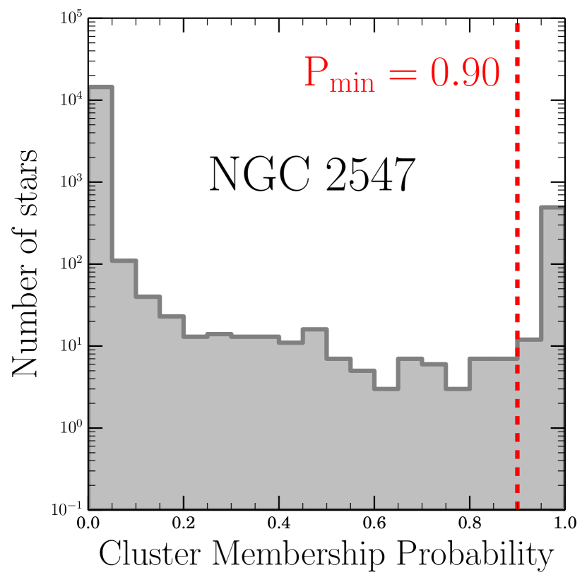
For NGC 2547, we find the distribution of cluster membership probabilities to be strongly bimodal, with most of the sample having probabilities close to either 0 or 1. Although not explicitly shown, the membership probability distribution has a strong dependence on the stars’ apparent $G$ band magnitude, with the distribution being mostly bimodal for bright stars, and becoming blurrier for fainter stars (with increasingly more stars having intermediate probability values; e.g., see Figure 5 of Jones & Prosser 1996). This magnitude-dependent outcome is typical, as bright stars tend to have more precise astrometric measurements, and the method provides a yes or no answer regarding their memberships. On the other hand, faint stars typically have larger astrometric uncertainties, which only allow the method to provide an intermediate answer.

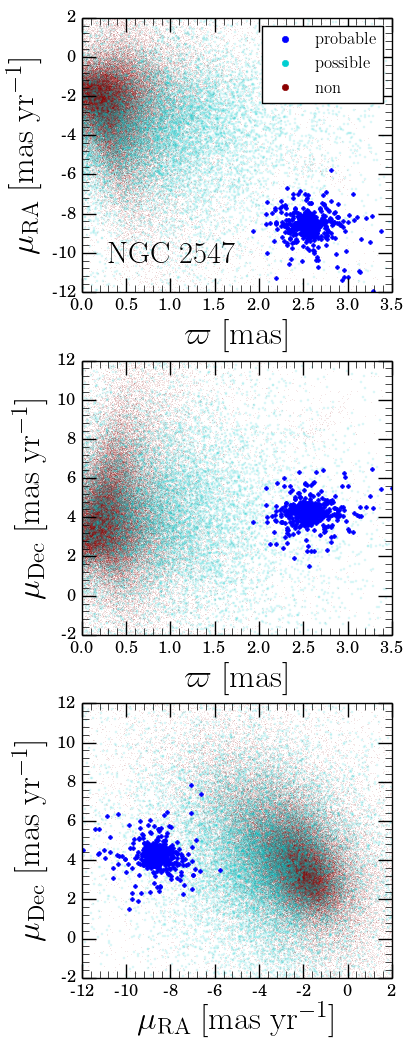
With this in mind, we apply a final selection criterion and classify the stars with $P_{C}\geq$ 0.90 as “probable members”, and those with $P_{C}<$ 0.90 as “possible members”. We show the resulting phase-space projections and apparent CMD of these populations, in addition to the “non member” population, in Figures 2 and 3. (The “no info” population is absent from these figures, as no astrometric information is available for those stars.)

Figure 2: NGC 2547: phase-space projections of the probable (blue), possible (cyan), and non (red) members defined in §3.1.3. The probable members are clustered in phase-space, while the non members (i.e., field stars) populate a much larger region at smaller parallax and proper motion values. The possible members correspond to an intermediate population, dominated by faint stars with large astrometric uncertainties.

We choose the probability threshold of $P_{\text{min}}=0.90$ to separate between probable and possible members as a compromise between completeness in our sample of probable cluster members on the one hand, and the presence of contamination on the other. Several tests with different $P_{\text{min}}$ values showed that the phase-space and CMD of the probable members seemed to lose bona fide cluster stars when using higher $P_{\text{min}}$ values, while lower values included stars with incoherent kinematics and photometry. We nonetheless note that the overall number of probable and possible members do not considerably change unless very high ($P_{\text{min}}\gtrsim$0.95) or very low ($P_{\text{min}}\lesssim$0.05) threshold values are used (see Figure 1). Furthermore, Appendix C reports the Gaia data for the probable and possible members and their cluster membership probabilities, and the reader is free to experiment with customized threshold values.

Figure 2 shows that the probable members (blue points) tend to be clustered in phase-space with a small number of stars located in the outskirts. On the other hand, the non members (i.e., the field; red points) occupy a much larger region in the phase-space projections (with stars populating virtually all corners of the diagrams), but tend to be concentrated at smaller parallax and proper motion values. The possible members (cyan points) appear as an intermediate population of stars, located in between the cluster and the field.

Figure 3: NGC 2547: apparent $G$ band versus $G_{\text{BP}}-G_{\text{RP}}$ CMD of probable (blue), possible (cyan), and non (red) members defined in §3.1.3. Although no photometric selection criteria was used to define the three populations, the probable members form an isochrone-like sequence, confirming that our selection method is identifying likely cluster members. The non members show the typical behavior of the background field, while the possible members mainly consist of faint stars ($G\gtrsim$ 19.5 mag). The “turnover” to bluer colors for apparent $G\gtrsim$ 18.5 mag for the probable members sequence is discussed in §3.1.3. The dotted and dashed lines show the $G=$ 17.5 and 18.5 mag limits, which we use to define different regimes in our mass and temperature calculation (see §4.2).

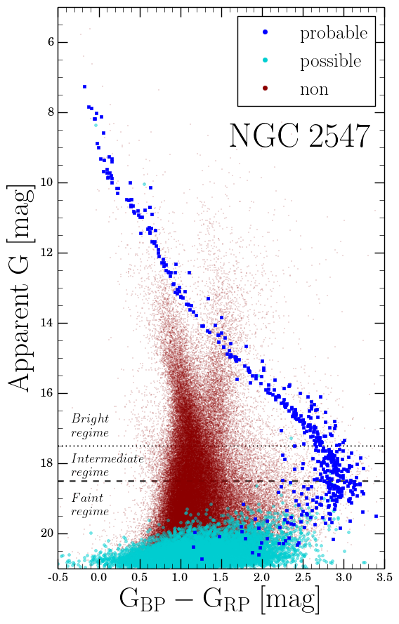
Figure 3 complements what is seen in Figure 2. The probable members form a tight isochrone-like sequence in the apparent CMD (with the exception of the color turnover for apparent $G\gtrsim$ 18.5 mag; see discussion below), with even a parallel sequence being visible indicating the presence of photometric binaries (e.g., Hurley & Tout 1998). The non members behave as expected from the field, with the two main branches (main-sequence and giant branch) being clearly visible in the data. The possible members mainly populate the bottom part of the plot, demonstrating that this population is dominated by faint stars that, consequently, have large astrometric uncertainties, which in turn causes them to have $\Delta_{i}\leq 3$ values (differentiating them from the non members). While some of these possible members could very well be real cluster members, the current precision of their astrometric information does not allow for a more stringent classification.

We highlight that even though our classification method is completely agnostic to the photometry of the stars, and it is solely based on kinematics, it seems to appropriately select stars that form a main-sequence in the CMD. We take this as a confirmation that our method is properly identifying likely cluster members and distinguishing them from the field.

A peculiar feature can be seen in Figure 3 for apparent $G\gtrsim$ 18.5 mag. At this apparent magnitude, instead of continuing to the bottom-right part of the diagram, the probable members start to turn to bluer colors for fainter magnitudes. This feature has already been found by other works when using the Gaia DR2 photometry (e.g., Arenou et al. 2018; Lodieu et al. 2019a, b; Smart et al. 2019), and it arises from an overestimation of the flux in the $G_{\text{BP}}$ passband for faint, red sources (Riello et al., 2018, 2021).

3.2 Crossmatch

Now that we have kinematically classified every Gaia DR2 star in the field of NGC 2547 as either a probable, possible, or non member, or a no info star, we proceed to connect this with the rotation sample of Irwin et al. (2008).

We crossmatch both catalogs using the CDS X-Match Service on VizieR. First, we download all the Gaia DR2 matches to a given NGC 2547 star within 3″. This produces matches for all stars, with some of them ($\sim$ 10%) being matched to two Gaia sources. The distribution of angular separations is strongly peaked at small values, with $\sim$ 80% of the stars having a match within 0.2″, a tail extending out to 0.5″, and some matches extending past this value out to 3″.

To select the best possible matches for stars matched to two Gaia sources, we compare the $V$ magnitudes from Irwin et al. (2008) with the $G$ magnitudes from Gaia. This exercise helps us break the ties and decide which star is the correct match. In all cases, the Gaia star with the more similar brightness corresponds to the closer match in angular separation. The second matched star is typically several magnitudes fainter, with angular separations greater than 1″ (the outliers of the separation distribution). We only keep one Gaia match per star, and are left with an angular separation distribution where $\sim$ 95% of the stars have a match within 0.3″, and all of them have a match within 0.9″.

In order to test the reliability of our crossmatching approach, we use the Pleiades cluster as a benchmark for which a completely independent crossmatching is available. We first replicate the same crossmatching procedure used in NGC 2547 with our Pleiades data. We then take the 2MASS IDs for the Pleiades stars from Rebull et al. (2016a), and look them up in the precomputed 2MASS-Gaia DR2 crossmatch (gaiadr2.tmass_best_neighbor) that can be found in the ESA’s webpage of the Gaia Archive. We find an excellent agreement ($>$ 99.7% of coincidence) between ESA’s crossmatch and ours for the stars found by both methods (and moreover, VizieR produces matches for 10 Pleiades stars not found by ESA). We take this as a confirmation that our crossmatching is properly combining the periodic samples with the Gaia sources.

3.3 Applying our Method to all the Clusters

We follow the method described in §3.1 for NGC 2547, and apply it to the other six clusters listed in Table 1. We report the astrometric parameters we calculate for the clusters in Appendix B, where we also compare them with the values reported in the literature. We find our astrometric parameters to be in good agreement with those reported by other studies, with fractional differences being typically at the $\sim$1–2% level or less.

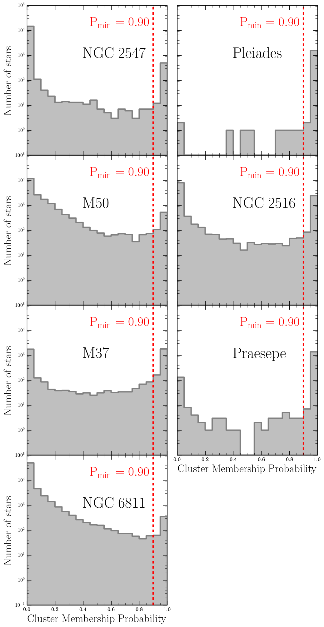
For each cluster, we classify every Gaia star contained within the region where the corresponding rotation period catalog reports candidate members, into one of the four previously described categories (no info, probable, possible, or non member). We report tables with the corresponding list of probable and possible members for every cluster in Appendix C. Analogously to Figures 1 and 3 for NGC 2547, Figures 4 and 5 show the membership probability distribution and apparent CMDs for all the clusters we study. The phase-space projections for all clusters, analogous to Figure 2 for NGC 2547, can be found in Appendix D.

Figure 4 shows that, for every cluster, in the sample of Gaia stars that satisfy $\Delta_{i}\leq$ 3, there is a population of stars with membership probabilities close to 1. This population represents a set of likely cluster members, and we classify those with $P_{C}\geq$ 0.90 as probable members (and the rest as possible members). On the low-probability end, however, clear cluster-by-cluster differences can be observed. While clusters such as the Pleiades and Praesepe show only a small number of possible members, M50 and NGC 6811 are in the opposite situation. These differences are explained by considering how similar or different the astrometric parameters of a given cluster are, compared with the field (which is typically a diffuse background population with small parallax and low proper motion). In other words, a cluster with a large parallax and proper motion (e.g., the Pleiades or Praesepe) will be more distinct and separated from the field in phase-space, and therefore it is highly unlikely that unassociated field stars will have similar astrometry (i.e., $\Delta_{i}\leq$ 3), and hence a small number of possible members is expected. On the other hand, field stars are more likely to mimic the astrometry of a cluster that has a small parallax and a low proper motion (e.g., M50 or NGC 6811), and therefore the number of stars that are kinematically consistent with the cluster increases.

Figure 4: Membership probability distribution for all the clusters we study, analogous to Figure 1.

Figure 5: Apparent $G$ band versus $G_{\text{BP}}-G_{\text{RP}}$ CMD of probable (blue), possible (cyan), and non (red) members for all the clusters we study, analogous to Figure 3.

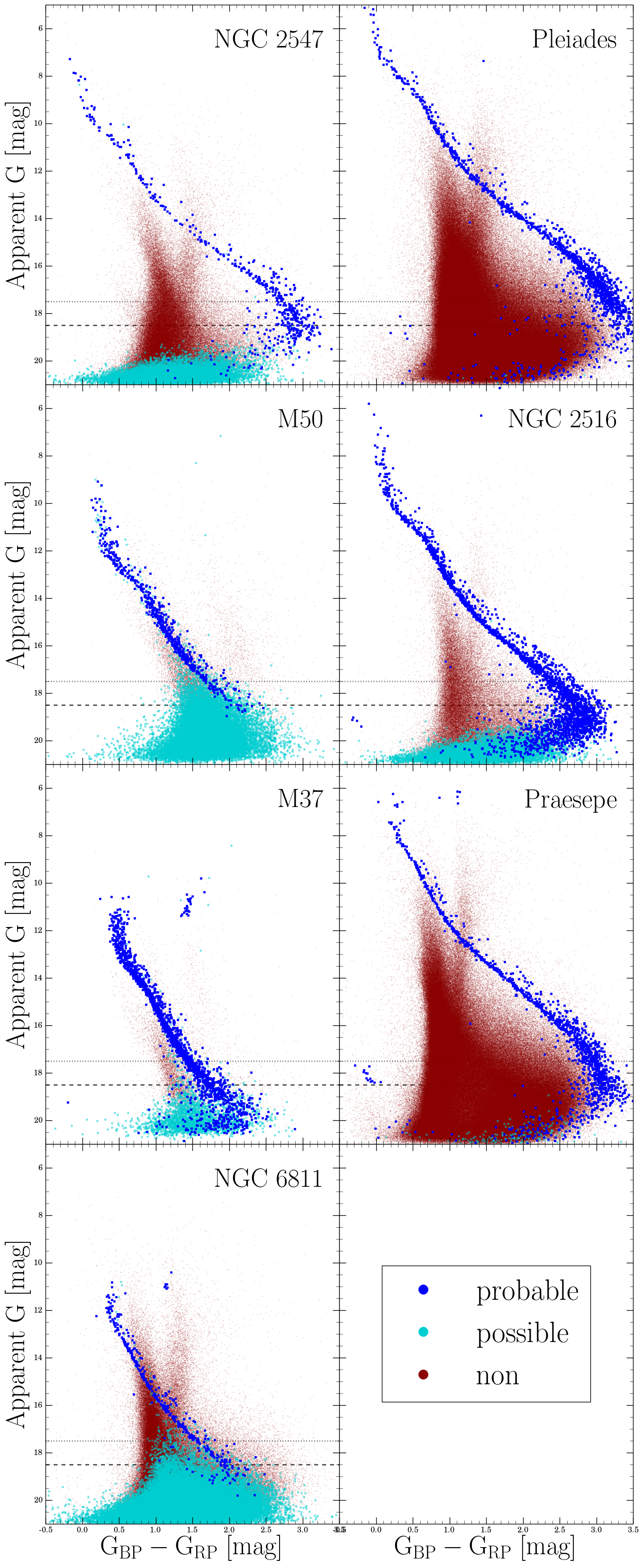
The apparent CMDs of all our clusters, shown in Figure 5, display an isochrone-like sequence of probable members, with clear binary sequences being identified in all of them. The older clusters M37, Praesepe, and NGC 6811 show not only a main-sequence population, but also a few giant stars (with Praesepe even showing a clear white dwarf sequence). We highlight that, in order to obtain unbiased cluster memberships, our method is completely agnostic to the Gaia photometry, and these results are a consequence of our careful astrometric analysis. Additionally, as previously found for NGC 2547, we observe the turn over to bluer $G_{\text{BP}}-G_{\text{RP}}$ colors at apparent magnitudes $G\gtrsim$ 18.5 mag in the probable member sequence of all the clusters. We take this as further evidence that this corresponds to an artifact of the Gaia photometry (see §3.1.3 for details).

As discussed in §3.1.3, our ability to cleanly separate between possible and probable members is a strong function of the stars’ apparent $G$ band magnitude, as the quality of their astrometry decreases with decreasing brightness. This can be clearly seen, for instance, in the CMD of NGC 6811, where all the stars fainter than apparent $G\simeq$ 19 mag are classified as either possible or non members, and none of them are classified as probable members. Real NGC 6811 members with $G>$ 19 mag are simply too faint for Gaia DR2 to provide precise astrometry, preventing us from reliably differentiating them from the field stars.

The crossmatching between the periodic samples and the Gaia DR2 data is done in identical fashion for all of the clusters, following the approach of §3.2. Unlike the case of NGC 2547, however, we do not find a Gaia DR2 counterpart for every periodic star in most of the other clusters. Our recovery rates (and number of stars not found in the crossmatching over the number of stars with measured periods) are: 100% (0/176) for NGC 2547, 99.9% (1/759) for Pleiades, 94.3% (46/812) for M50, 99.4% (2/364) for NGC 2516, 96.7% (12/367) for M37, 99.8% (2/809) for Praesepe, and 100% (0/232) for NGC 6811. The only clusters with recovery rates below 99% are M50 and M37, which correspond to distant systems where the periodic samples extend to magnitudes fainter than the apparent $G\approx 21$ mag limit of Gaia DR2. In the following, we classify the stars not found in the crossmatching as no info stars, as their membership is uncertain and we do not have evidence to discard them.

4 Cluster and Stellar Properties

4.1 Cluster Properties

To perform meaningful inter-cluster comparisons of stellar rotation, reliable cluster properties are needed. In the pre Gaia era, classic works such as Denissenkov et al. (2010), Gallet & Bouvier (2013), and Gallet & Bouvier (2015) thoroughly compiled periodic samples as well as properties for a large number of clusters. Nevertheless, the heterogeneous nature of their parameter compilation (adopting values from varied techniques and data sets), can result in inhomogeneities in the adopted masses, ages, and metallicity scales. Nowadays, the systematic observations of star clusters by spectroscopic surveys (Netopil et al. 2016; Gaia-ESO, Spina et al. 2017, Magrini et al. 2017; APOGEE, Majewski et al. 2017, Jönsson et al. 2020), as well as the uniform all-sky Gaia data, provide an opportunity to study these systems in a more consistent and homogeneous fashion. In the following, we attempt, to the extent that it is possible, to compile and derive cluster properties that are in a consistent and uniform scale.

The mass and temperature values we calculate in §4.2, as well as the results and discussion presented in §5 and §6, require four cluster properties to be known: distance modulus, reddening, age, and metallicity. The former two are needed to translate the observed photometry to absolute and dereddened CMD space, while the latter two are required to compare the data with the appropriate stellar evolutionary model. For distance modulus, we adopt the values derived from our astrometric analysis (considering the parallax zero-points described in §3.1.1), and for metallicity we compile values reported from recent high-resolution spectroscopic results. In particular, we adopt the state-of-the-art values reported by Netopil et al. (2016) for Pleiades, NGC 2516, M37, Praesepe, and NGC 6811, and the value reported by the Gaia-ESO survey (Spina et al., 2017) for NGC 2547. The only cluster without a spectroscopic metallicity measurement is M50, for which we adopt a solar value. We now describe our procedure to obtain cluster reddenings and ages.

Instead of adopting reddening values from the literature, we calculate our own using a dedicated fitting routine. For a given cluster, we start by correcting the observed $G$ band magnitudes by distance modulus. Once the spectroscopic metallicity is known, we download a set of PARSEC models (Bressan et al., 2012; Chen et al., 2014) of that composition with a range of plausible ages (e.g., 100, 200, and 300 Myr for NGC 2516). Then, we define a region in the absolute CMD where the different models agree with each other, which excludes the phases near and more evolved than the turnoff. We then iterate over a range of possible reddenings and find the value that produces the best agreement between the observed data with the series of models.

For a given $E(B-V)$ value, we assume $A_{V}=3.1\times E(B-V)$ (Cardelli et al., 1989) and deredden the photometry as follows. For stars with measured photometry in the three Gaia bands, we deredden the observed magnitudes following the approach of Gaia Collaboration et al. (2018b), where the extinction coefficients depend on $G_{\text{BP}}-G_{\text{RP}}$ color and extinction itself. For stars that lack a measured $G_{\text{BP}}-G_{\text{RP}}$ color, we adopt the PARSEC coefficients for a G2V star ($A_{G}/A_{V}=0.85926$, $A_{G_{\text{BP}}}/A_{V}=1.06794$, and $A_{G_{\text{RP}}}/A_{V}=0.65199$).

For every $E(B-V)$ value we are iterating over, we deredden the probable cluster members’ photometry, define a set of bins in the $(G_{\text{BP}}-G_{\text{RP}})_{0}$ color coordinate, and calculate the mean colors and 75th magnitude percentiles (which accounts for the photometric binaries). We then find the $E(B-V)$ value that minimizes the sum of the squared difference of the data minus the models given the bins, and adopt this as our global cluster reddening. Finally, we compare the CMD location of the full sample of probable members with models of varying ages, and estimate the age following the envelope of hot stars below and near the turn-off (typically stars hotter than $\sim$ 7,000 K). We estimate that this procedure leads to typical errors of $\sim 20\%$ for reddenings and $\sim$ 10–20% for ages.

We summarize the revised cluster properties we adopt in Table 2. Note that for the nearby and young clusters NGC 2547 and the Pleiades, we adopt the lithium-depletion ages from Jeffries & Oliveira (2005) (see also Naylor & Jeffries 2006) and Stauffer et al. (1998), respectively. This technique yields reliable and almost completely model-independent ages in the $10\textendash 200$ Myr range. These adopted ages are in good agreement with the values we derive from our CMD analysis.

Table 2: Revised and updated cluster properties.

Name	Age	[Fe/H]	DM	Distance	$E(B-V)$
-	[Myr]	[dex]	[mag]	[pc]	[mag]
NGC 2547	35	$-$0.01	7.925	384.6	0.044
Pleiades	125	$-$0.01	5.670	136.2	0.051
M50	150	0.00	9.936	970.9	0.210
NGC 2516	150	$+$0.05	8.058	408.8	0.103
M37	500	$+$0.02	10.787	1436.8	0.246
Praesepe	700	$+$0.16	6.345	185.8	0.014
NGC 6811	950	$+$0.03	10.167	1080.1	0.047

4.1.1 Comparing our Cluster Properties with the Literature

We now compare the cluster properties we have derived, with the values that can be found in the literature from similar approaches. The main references we use for this are Gaia Collaboration et al. (2018b) and Bossini et al. (2019), who also studied open clusters based on the Gaia DR2 data, and reported parameters for most of the clusters in our sample based on comparisons with PARSEC models. We also use as reference the works by Cummings et al. (2016), Cummings & Kalirai (2018), and Cummings et al. (2018). Although these did not use Gaia data, they reported parameters for many of the clusters in our sample based on CMD fits to $UBV$ photometry and PARSEC models.

For distance modulus, our values are calculated from the global cluster parallaxes, accounting for a zero-point value of 53 $\mu$as in NGC 6811 and of 29 $\mu$as for the other clusters. While Gaia Collaboration et al. (2018b) and Bossini et al. (2019) (whose membership and astrometry come from Cantat-Gaudin et al. 2018) do not consider these zero-points, in Appendix B we add these offsets to their parallax values for an appropriate comparison, and find differences to be within $\approx\pm 1$%. For metallicity, we share references and use high-resolution spectroscopic values from Netopil et al. (2016) or Gaia-ESO when available.

For reddening, if we exclude M50 from the comparison, we find good agreement with Gaia Collaboration et al. (2018b) and Bossini et al. (2019), and the differences between our values and theirs are contained within $\pm 0.032$ mag in $E(B-V)$. On the other hand, M50 is the only cluster for which the Gaia Collaboration et al. (2018b) and Bossini et al. (2019) reddenings differ between each other. The former reports $E(B-V)=0.105$ mag, the latter reports 0.153 mag, and we obtain a best-fit value of 0.210 mag. We note, however, that Cummings et al. (2016) and Cummings & Kalirai (2018) report $E(B-V)=0.230$ for M50, in better agreement with our estimate. Ultimately, the above differences in reddening are perhaps unsurprising considering the different CMD analysis approaches and parallax zero-point considerations.

Regarding stellar ages, we find our revised values to be in good agreement with the pre Gaia values compiled by Gallet & Bouvier (2015) listed in Table 1 (see also Denissenkov et al. 2010; Gallet & Bouvier 2013), especially considering the associated uncertainties. The largest difference is seen for Praesepe, for which we derive an age of 700 Myr, while Gallet & Bouvier (2015) adopt 580 Myr. Given the crucial importance that clusters’ ages play in models of angular momentum evolution, the overall good agreement between our values and the pre Gaia ones is a meaningful result of our work.

Comparing our ages with those by Gaia Collaboration et al. (2018b), we find our results to be in good agreement. A similar comparison with Bossini et al. (2019) shows that their ages seem to be systematically underestimated by factors of $30\textendash 60\%$ for the younger clusters. The exception to the above is NGC 2516, for which Gaia Collaboration et al. (2018b) and Bossini et al. (2019) report ages of $\approx$ 300 and 250 Myr, respectively. If confirmed, this would position NGC 2516 as an important anchor for stellar rotation at intermediate ages, as few systems older than the Pleiades and younger than M37 have such comprehensive periodic data sets. Nevertheless, our analysis favors the classical $\sim$ 150 Myr age, and this value is similar to the results by Cummings et al. (2016), Cummings & Kalirai (2018), and Cummings et al. (2018) (see also Fritzewski et al. 2020, Healy & McCullough 2020, and Bouma et al. 2021).

4.2 Stellar Properties

In order to perform comprehensive comparisons of the rotational sequences of the open clusters, we need to place them on a common scale. For this, we derive mass and temperature values for the cluster members by comparing the photometric data with state-of-the-art evolutionary models in absolute magnitude space. Although the papers that reported periods also reported photometry in at least two bands for most of our clusters (e.g., $V$ and $I$ for NGC 2547; see §2), the specific filters vary on a cluster by cluster basis. Instead of using these, we take advantage of the uniform $G$, $G_{\text{BP}}$, and $G_{\text{RP}}$ photometry provided by Gaia DR2. This also allows us to derive masses and temperatures for all the Gaia cluster members, not just the subset with measured periods.

We again illustrate our procedure using NGC 2547 as a working example. We use its $E(B-V)$ and distance modulus values (see §4.1) and calculate absolute and dereddened photometry. We show the extinction-corrected absolute CMD of the probable and possible NGC 2547 members in Figure 6. The data can now be directly compared with stellar models to infer mass and temperature values. We use a PARSEC isochrone with the corresponding NGC 2547 age and metallicity, and show it as the orange line in Figure 6.

The bright probable cluster members show an excellent agreement with the model in Figure 6. As discussed in Figure 3, the $G_{\text{BP}}-G_{\text{RP}}$ color misbehaves for apparent $G\gtrsim 18.5$ mag, and the probable member sequence becomes bluer for fainter magnitudes. This limit is translated to the absolute and dereddened CMD and shown as the horizontal dashed line in Figure 6, with the dotted line showing a similar apparent $G=17.5$ mag limit. We use these two apparent magnitude limits, here translated to absolute magnitude space, to define different regimes in our mass and temperature calculation.

Figure 6: NGC 2547: absolute and dereddened CMD of the probable (blue) and possible (cyan) members. The points from Figure 3 have been corrected by extinction and distance modulus. The best-fit NGC 2547 PARSEC isochrone is shown as the orange line. The dotted and dashed lines correspond to the apparent $G=$ 17.5 and 18.5 mag limits from Figure 3 translated to absolute CMD space, which define different regimes in our calculation. We use this figure to interpolate the model and derive mass and temperature values (see §4.2).

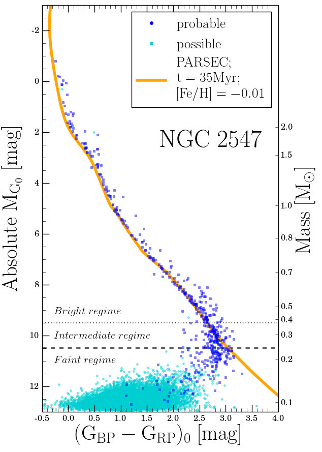
Additionally, whenever possible, the effects of binarity on the CMD need to be considered. Photometric binaries appear as brighter/redder stars compared to the main-sequence locus, and to account for them we follow the procedures of Stauffer et al. (2016) and Somers et al. (2017). In this approach, when the Gaia $(G_{\text{BP}}-G_{\text{RP}})_{0}$ color is reliable, stars are projected down (or up) onto the main-sequence locus at fixed color, effectively removing the contribution of close companions (i.e., our mass and temperature estimates for these stars correspond to those of the primary star). We designate the projected absolute magnitudes as $M_{G_{0,proj}}$, and describe its calculation in detail below.

To acknowledge the misbehavior of the $G_{\text{BP}}-G_{\text{RP}}$ color and account for the contribution of photometric binaries when possible, we define three regimes to calculate projected magnitudes $M_{G_{0,proj}}$ in the absolute CMD of Figure 6:

• Bright regime: For stars brighter than the dotted line (apparent $G=17.5$ mag translated to absolute magnitude), we calculate $M_{G_{0,proj}}$ by projecting the stars $M_{G_{0}}$ value down (or up) onto the model at the measured $(G_{\text{BP}}-G_{\text{RP}})_{0}$ color.

• Faint regime: For stars fainter than the dashed line (apparent $G=18.5$ mag translated to absolute magnitude), or stars that lack a $G_{\text{BP}}$ or $G_{\text{RP}}$ magnitude, we cannot rely on the $(G_{\text{BP}}-G_{\text{RP}})_{0}$ color to do a de-projection. Instead, we simply keep the calculated $M_{G_{0}}$ value as is, and define $M_{G_{0,proj}}$ to be equal to it. This is therefore a regime where we do not account for unresolved companions.

• Intermediate regime: For stars in between the dotted and dashed lines ($17.5\leq G\leq 18.5$ mag range translated to absolute magnitude), we do an intermediate, ramp-like calculation. We calculate the values we would have obtained following the bright and faint regimes separately, and combine them in a progressive way with linear weighting. In this way, the extremes match the corresponding methods, effectively avoiding a sharp transition between the different regimes.

For every star, this procedure collapses the observed photometry to the single quantity $M_{G_{0,proj}}$. We use this value to interpolate the corresponding NGC 2547 PARSEC model in the magnitude-mass and magnitude-temperature space. We only interpolate in the regime of stars fainter than the main-sequence turnoff (i.e., we do not report masses for evolved stars) and down to the faintest $M_{G_{0}}$ magnitude allowed by the model. We report our derived masses and temperatures for the NGC 2547 probable and possible members in Appendix C.

For the subset of NGC 2547 stars with period measurements, Irwin et al. (2008) calculated masses using their $I$ band magnitudes and the NextGen models (Baraffe et al., 1998). These values offer a completely independent reference point to validate our own masses, and we compare our estimates with theirs in Figure 7. It is important to highlight one key difference between both methods: we account for the presence of photometric binaries (when possible), while Irwin et al. (2008) do not. Accordingly, we find the mass difference to be a strong function of mass itself. For stars in the faint regime, where we do not account for binaries, we see a good agreement but with an approximately constant offset of $\Delta$Mass $\approx-0.05M_{\odot}$ that is likely due to the different underlying models used in the interpolation. For higher masses, the scatter increases and many stars have positive mass differences, indicating cases where Irwin et al. (2008) did not account for the contribution of unresolved companions. Overall, we find a good agreement, with mean and standard deviation values of $\Delta$Mass being $\approx$ 0.01 and 0.08 $M_{\odot}$, respectively.

Figure 7: NGC 2547: Comparison of our mass estimates with those of Irwin et al. (2008) for the stars in the periodic sample. We show mass difference (in the sense of Irwin et al. (2008) minus this work) versus mass from this work. Both estimates come from entirely independent photometric data sets and interpolated models. The dotted and dashed lines correspond to the apparent $G=$ 17.5 and 18.5 mag limits from Figure 3 translated to mass coordinates, and these values define the three regimes used for our mass calculation. We find a good overall agreement, and the comparison suggests a possible systematic uncertainty of $\sim$ 0.05 $M_{\odot}$ in the masses derived by this method. In the intermediate and bright regimes, the Irwin et al. (2008) masses tend to be higher due to their method not accounting for photometric binaries.

Figure 8: Absolute and dereddened CMD of the probable (blue) and possible (cyan) members for all the clusters we study, analogous to Figure 6. The orange lines are the respective best-fit PARSEC isochrones.

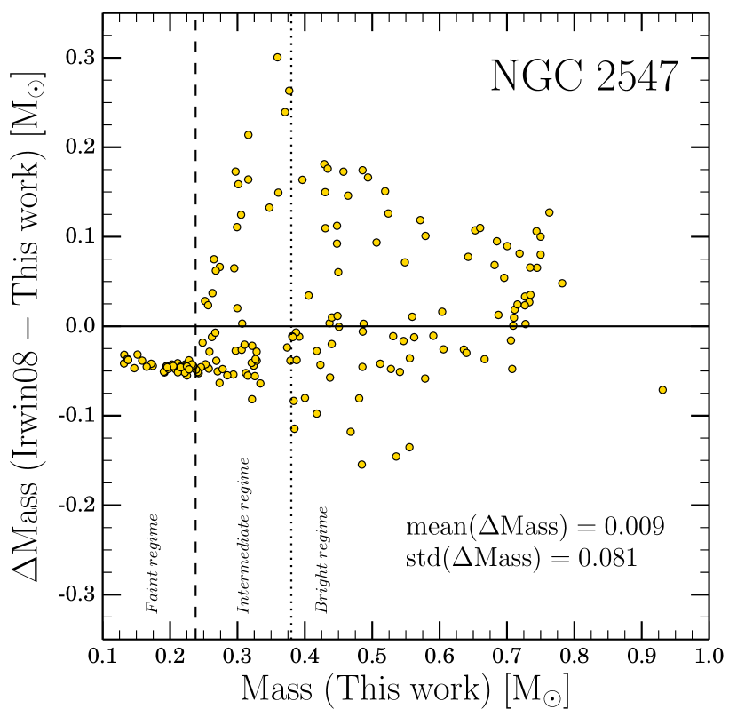
The above comparison validates our method, and suggests that masses derived in this way are subject to a systematic uncertainty of order $\sim$ 0.05 $M_{\odot}$. Statistical uncertainties are of order $\sim$ 0.01–0.02 $M_{\odot}$, considerably smaller than the systematic ones. More importantly, by using the Gaia photometry, we have defined a procedure to calculate the masses and temperatures that can be uniformly applied to all our clusters.

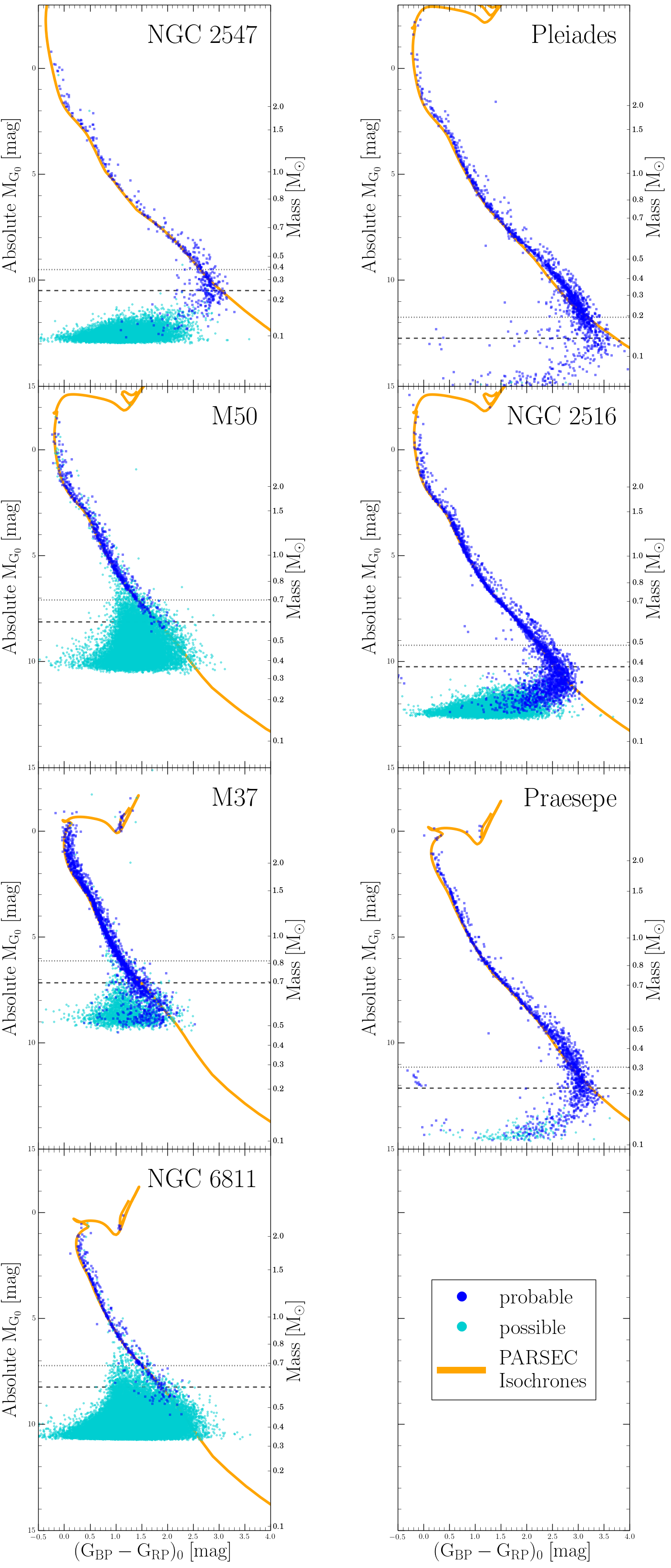
Analogously to Figure 6 for NGC 2547, Figure 8 shows the extinction-corrected absolute CMD for the probable and possible members of all the clusters. Some discrepancies arise for low mass stars, where the probable members appear brighter/redder than the model (e.g., see the $\sim 0.4M_{\odot}$ stars in Pleiades and Praesepe). As other studies suggest, these differences could arise due to the known radius inflation problem in cool dwarfs (e.g., Torres & Ribas 2002; Clausen et al. 2009; Torres et al. 2010; Kraus et al. 2011; Somers & Stassun 2017; Jackson et al. 2018, 2019). Accounting for the underlying physical process that causes this in the models is beyond the scope of this paper, but we refer interested readers to the works by Somers & Pinsonneault (2015) and Somers et al. (2020). Regardless, while evidently not perfect, Figure 8 shows a good overall agreement of the data with models across the HR diagram for all the clusters.

We follow the procedure described for NGC 2547, and use the absolute CMDs to calculate masses and temperatures for the probable and possible cluster members. We report these values in Appendix C. For the subset of stars with independent mass and temperature estimates from other studies, we compare these values with ours in Appendix E. Globally, we find our masses and temperatures to be in good agreement with those reported by the period references. The comparisons suggest possible systematic uncertainties of $\sim 0.05\textendash 0.1M_{\odot}$ in mass and $\sim 150$ K in temperature, which are modest considering the different methods, photometric data, and underlying stellar models employed.

5 Results

For the remainder of this paper we focus on the subset of main-sequence stars with period measurements, the periodic samples. Particularly, in this section we proceed to investigate how the clusters’ rotational sequences change when we consider the astrometric classifications previously derived, to what extent field contamination is an issue, and whether rotational outliers are real cluster members. For this, we remove from our sample all the Pleiades and Praesepe stars that Rebull et al. (2016b) and Rebull et al. (2017) classify as pulsators, as well as the giant NGC 6811 stars for which Santos et al. (2021) report rotation periods (which are longer than 100 days). Additionally, for the Pleiades and Praesepe stars with multiple period measurements, we only consider their main periods as the adopted rotation period ($P1$ from Rebull et al. 2016a, b and Rebull et al. 2017). Tables with the membership classifications and periods, as well as other important parameters (e.g., Gaia DR2 IDs, derived masses and temperatures, membership probabilities) for the periodic samples are reported in Appendix F.

Figure 9 shows the results of applying our astrometric classification to the rotational sequences of the periodic samples. For each cluster, we show both the literature sequence (i.e., pre Gaia DR2 membership analysis), and its revised version reported in this work (i.e., post Gaia DR2). The literature rotational sequences (left column) include all the candidate cluster members reported in the original period references, and we color code them according to our astrometric classifications. The revised sequences (right column), only show probable members, possible members, and no info stars, but do not show stars classified as non members. Since at this point we have no means to either confirm or reject the membership status of the no info stars, we simply add them to the possible members category in the revised sequences of Figure 9.

Figure 9: Period versus temperature diagrams for all the clusters we study. For each cluster we show two panels: the literature sequence (i.e., pre Gaia DR2 membership analysis; left panel) and its revised version reported in this work (i.e., post Gaia DR2; right panel). The literature sequences show all the stars reported in the original period references, and we color code them according to our astrometric classification: no info star (open black pentagons), non member (red squares), possible member (open cyan diamonds), or probable member (blue circles). The number of stars in each category is shown in the parenthesis accompanying the labels. In the revised sequences we do not show the non members to demonstrate the effects of removing the field contamination, and we combine the no info stars with the possible members (open green diamonds). The dotted and dashed lines correspond to the apparent $G=17.5$ and 18.5 mag limits from Figure 5 translated to $T_{\text{eff}}$ coordinates. We observe varying degrees of non member contamination, with the clusters observed from the ground showing higher rates, and the more distant clusters having more uncertain revised sequences (see §5 and §6).

Before comparing the literature and revised rotational sequences in detail, we note that a strong artifact inherited from the Gaia astrometry is present in the membership classification of our most distant clusters. In M50 (distance of $\sim$ 970 pc), for $T_{\text{eff}}\gtrsim 4500$ K, most of the stars are classified as either probable or non members. On the other hand, stars cooler than this limit are mostly classified as possible members (and furthermore, for $T_{\text{eff}}\lesssim 3500$ K the predominant category is no info stars). This is a direct consequence of the quality of the Gaia astrometry decreasing monotonically for fainter, cooler targets, where our classification method can no longer reliably identify probable or non members, and we instead classify most stars as possible members. A similar effect is observed in M37 (distance of $\sim$ 1440 pc), with the limit being around $T_{\text{eff}}\simeq 4000$ K. This effect is absent in the rotational sequence of NGC 6811 (distance of $\sim$ 1080 pc), but only because the periodic sample does not extend to such faint, cool stars.

We now examine Figure 9 in detail and discuss how the inclusion of the astrometric information affects the rotational sequence of each cluster independently:

• NGC 2547: for this cluster we classify $\sim$ 25% of the Irwin et al. (2008) candidates as non members. By removing this contamination, the rotational sequence changes considerably. At a given $T_{\text{eff}}$, most of the non members actually correspond to stars with the longest periods, and after including our membership analysis, only 2 stars with period $>$ 10 days remain (one of them a probable member, while the other a no info star). Interestingly, the revised NGC 2547 sequence exhibits strong $T_{\text{eff}}$- and mass-dependent trends in the period distribution, with the mean period decreasing with decreasing $T_{\text{eff}}$ for $T_{\text{eff}}<3500$ K. Given its young age ($\sim$ 35 Myr), we expect the period versus $T_{\text{eff}}$ distribution of NGC 2547 to be strongly affected by processes that regulate stellar rotation at birth.

• Pleiades: we find the non member contamination to be small ($\lesssim$ 4%), and that removing it, for the most part, does not empty specific regions in the rotational sequence. This finding is not surprising, as the Pleiades stars studied with K2 by Rebull et al. (2016a), Rebull et al. (2016b) and Stauffer et al. (2016) had been previously vetted by proper motion surveys. Further examination of the stars classified as non members reveals that $\approx$ 70% of them have $\Delta_{i}$ values between 3 and 5 (i.e., are outside the cluster’s $3\sigma$ ellipsoid in phase-space, but within $5\sigma$), suggesting that a less stringent astrometric selection could have classified them as possible cluster members. Additionally, for the Pleiades we observe an interesting phenomenon (also observed in Praesepe): there is a large number of no info stars across the entire $T_{\text{eff}}$ range. This is noticeably different from the cases of M50 and M37, where the no info stars are heavily concentrated at the faint, cool end of the distributions. We further discuss this in §6, but in short, these no info stars mainly correspond to photometric binaries, which points to biases in the Gaia DR2 astrometry.

• M50: this cluster shows the largest differences of all when we compare the literature and revised rotational sequences. For $T_{\text{eff}}>4500$ K, we find the literature sequence to have substantial non member contamination ($\approx 36\%$), and we observe that the different astrometric populations occupy particular regions of the rotational sequence. Firstly, we note that all of the stars with periods $\lesssim$ 0.1 day are cleanly identified as non members. This is perhaps not surprising, as these periods most certainly do not correspond to rotational signals but rather pulsation signals from field stars. Secondly, we note that most of the long period stars ($\gtrsim$ 10 days) are actually classified as non members. Thirdly, after removing the field contamination, the probable members do form a rather clean sequence of rotation period as a function of $T_{\text{eff}}$, and both branches of slowly and rapidly rotating stars observed in the Pleiades can now be seen in the revised M50 sequence. For $T_{\text{eff}}\lesssim 4000$ K, the quality of the Gaia DR2 astrometry does not allow us to classify stars reliably, but we expect the contamination fraction to be of similar or higher significance than that of stars with $T_{\text{eff}}>4500$. Given how uncertain this part of the diagram is, in the analysis that follows we simply discard the M50 stars cooler than $\sim$ 4000 K (vertical dashed line in Figure 9, i.e., the apparent $G=18.5$ mag limit translated to $T_{\text{eff}}$ coordinate), and only consider the stars hotter than this limit.

• NGC 2516: this cluster shows a very low contamination rate, with only $\approx 3\%$ of the stars being classified as non members, and $\approx 88\%$ of the Irwin et al. (2007a) stars being classified as probable members. We suspect this arises from the fact that this cluster is very rich and therefore dominates (in terms of number counts; see Figure 5) over the field population in the CMD selection done by Irwin et al. (2007a). Accordingly, both literature and revised rotational sequences are almost identical, with the period distribution showing strong mass dependent trends. We note, however, that the periodic NGC 2516 stars span a narrow range in temperature (and mass), and the sample is limited to $T_{\text{eff}}<4400$ K ($M<0.7M_{\odot}$).

• M37: for $T_{\text{eff}}\gtrsim 4000$ K, we find the non member contamination to be $\approx$ 4%, which is small compared to the $\sim 20\%$ contamination rate expected by Hartman et al. (2008b). Similarly to NGC 2516, we think this arises from the richness of the cluster compared to the field, in addition to the double CMD selection done by Hartman et al. (2008b). Interestingly, however, the locations of many of the non members do not seem to be arbitrary. Most of them are stars that lie well off of the converged period sequence (at both longer and shorter periods), and are clearly separated from the probable members in the rotational sequence. This result implies that the converged sequence at this age ($\sim$ 500 Myr; §4) is actually stronger than previously thought. We note, nonetheless, that a few rotational outliers still survive the astrometric selection at both longer and shorter periods than the converged sequence. Additionally, and similarly to M50, M37 also exhibits a clear break in the astrometric classification, in this case around 4000 K. For stars cooler than this limit, our method cannot confidently separate probable members from non members, and we instead classify most of them as possible members or no info stars. Nevertheless, and in contrast to M50, given how clean the Hartman et al. (2008b) membership was in the $T_{\text{eff}}\gtrsim 4000$ K regime, we expect most of the stars cooler than this value to be real M37 members, and we do include them in the analysis that follows.

• Praesepe: the non members correspond to $\approx$ 7% of the sample, and this small contamination rate is not surprising given the previous CMD and proper motion vetting in the K2 stars studied by Rebull et al. (2017). Further examination of these non member stars reveals that $\approx$ 40% of them have $\Delta_{i}$ values between 3 and 5, and therefore a less stringent astrometric selection could have classified them as possible cluster members. Similarly to the Pleiades, the non members do not seem to empty specific regions in the rotational sequence, with the exception of the stars located in the $4300<T_{\text{eff}}<5500$ K range. Many of these non members have longer periods than the converged sequence, and the revised rotational sequence appears narrower than previously thought for this $T_{\text{eff}}$ range at this age ($\sim$ 700 Myr; §4). We find this result to be similar to that of M37, hinting to a convergence of rotation rates that is considerably stronger than previously thought (see §6). Nonetheless, we also note that a few rotational outliers survive the astrometric analysis and are still present in the revised sequence. Finally, and similarly to the Pleiades, we find that the no info Praesepe stars populate the entire $T_{\text{eff}}$ range of the sequence. These stars mostly appear as photometric binaries in the CMD, and we further discuss them in §6.

• NGC 6811: this cluster shows a very low contamination rate, with only $\approx$ 2% of the stars being classified as non members. This is consistent with expectations, given the samples that the NGC 6811 rotation period catalogs were based on. Meibom et al. (2011b) vetted stars on the basis of RV data, Curtis et al. (2019a) combined CMD selections with a set of astrometric cuts to ensure consistency with the cluster’s phase-space projections (although they did not take the stars’ uncertainties or intrinsic cluster dispersion into account), and Santos et al. (2021) performed their lightcurve analysis based on our sample of probable members. While all of the above work together to produce a low contamination rate by construction, three of the five stars classified as non members are clear outliers when compared with the probable members sequence. Similar to what we see in the other old clusters (M37 and Praesepe), however, the revised sequence does show a number of long period outliers, hinting to a rare channel that produces slow rotation for a small fraction of members in $\gtrsim 0.5$ Gyr-old clusters.

Finally, we point out a feature that is ubiquitous in all the clusters we study: the revised rotational sequences show a number of rapid rotators that survive all the astrometric cuts. These are stars that likely correspond to synchronized binaries, and they stand out more clearly in the older M37, Praesepe, and NGC 6811 clusters with periods of $0.5\textendash 2$ days and $5000<T_{\text{eff}}<6000$ K.

After having analyzed how the clusters’ rotational sequences change when the non member contamination is excluded, we emphasize that properly accounting for cluster membership remains a fundamental piece of empirical studies of stellar rotation. Incorrect or biased conclusions could be derived from rotational sequences that lack the appropriate vetting. Replicating our analysis with improved astrometry should further refine the astrometric classifications, and expand the mass and temperature range where the probable and non members can be reliably distinguished from each other.

6 Discussion

In this section, we use the periodic samples to study stellar rotation as a function of mass and age.

6.1 Rotation Data in the Gaia Era

At this point, for every cluster in our sample, we have classified the periodic stars using our astrometric analysis (§3), presented a set of revised properties that are needed to perform meaningful inter-cluster comparisons (§4), and discussed the effects that removing the field contamination has on the individual rotational sequences (§5). Now, we combine all of these to construct an updated portrait of the evolution of stellar rotation.

We illustrate this in Figure 10, where we show the revised period versus mass diagrams as a function of age. The color-coding is the same as the revised sequences of Figure 9, and the non member contaminants have been removed. This represents the state-of-the-art for rotation studies in terms of clean samples with stellar masses, temperatures, and ages derived in a consistent scale. We make these data publicly available in Appendix F.

Figure 10: Revised period versus mass diagrams for all the clusters we study (i.e., after having removed the non member contamination). The clusters are sorted by age, and the ages and masses are the values calculated in §4.2. The points are color-coded in the same fashion as the revised sequences of Figure 9. The dotted and dashed lines correspond to the apparent $G=17.5$ and 18.5 mag limits from Figure 5 translated to mass coordinates. To aid inter-cluster comparisons, in some panels we add an additional cluster in grey in the background. This figure represents the state-of-the-art data for studies of stellar rotation (see §6.1).

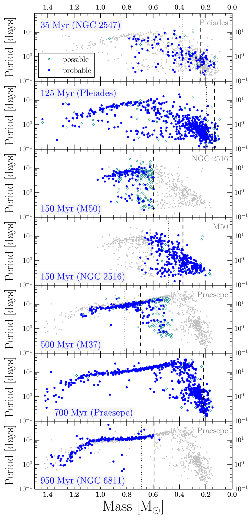
One of the major results of our study can be seen in the rotational sequence of M50 in Figure 10. When the non member contamination is removed, the revised M50 sequence clearly resembles that of the Pleiades, as we would expect given their similar ages (150 and 125 Myr, respectively). Incidentally, the low mass end of the M50 sequence coincides with the high-mass end of the co-eval NGC 2516 sequence ($\approx$ 0.65 $M_{\odot}$). This is illustrated in their respective panels, where we show the M50 sequence in blue and green, and the NGC 2516 sequence in grey, and vice versa. Given their indistinguishable ages, the merged M50 and NGC 2516 data can provide a valuable comparison point for the benchmark Pleiades cluster. Likewise, a similar comparison can be made for the older M37 and Praesepe clusters. Ultimately, the above demonstrates a decisive finding: when careful membership analysis are performed, the rotational sequences that have been constructed from ground-based observations (e.g., M50 by Irwin et al. 2009), can be as informative for stellar rotation studies as those constructed from space-based observations (e.g., the Pleiades by Rebull et al. 2016a). In this context, future dedicated ground-based monitoring combined with careful astrometric selections using Gaia could provide unprecedented constraints for angular momentum evolution (e.g., Curtis et al. 2020). This conclusion is particularly relevant in the post Kepler and K2 era, and considering that only a fraction of the TESS targets are being observed with long baselines.

Regarding the field contaminants, our membership analysis yields varying degrees of contamination rates. As mentioned in §2, we expected the clusters observed from the ground to show higher contamination rates compared to those observed from space. This turns out to be the case for NGC 2547 and M50, where we find the contamination to be $\approx$ 25% and 36%, respectively. While high, these values are lower than the $\sim 40\textendash 60\%$ rates anticipated by Irwin et al. (2008) and Irwin et al. (2009), which were based on predictions from Galactic models. For the rest of the sample we find the contamination rates to be lower, of order $\lesssim 5\%$ (see §5).

Interestingly, although our membership study has predominantly removed rotational outliers at both long and short periods for several clusters, many outliers are nonetheless classified as probable members and remain in the revised sequences. An interesting example of this are the slowly rotating stars (periods $\approx 7\textendash 10$ days) in the young NGC 2547 (age of $\sim$ 35 Myr), which hints to strongly mass-dependent initial conditions for stellar rotation (see also Somers et al. 2017; Rebull et al. 2018, 2020). Similarly, all three $\gtrsim 0.5$ Gyr-old clusters show confirmed members that are rotating faster ($\sim$ 1 day) and slower ($\sim$ 20 days) than their slowly rotating branches. Now that the membership status of these outliers have been confirmed, their presence can no longer be ignored or attributed to field contaminants.

The rapid rotators in systems with a converged sequence cannot be explained by single star evolution in current models. The most plausible explanation is that they have experienced tidal synchronization or are merger products. Regarding the slowly rotating outliers, a quick inspection reveals that most appear as typical cluster members in astrometric and photometric regards, but a fraction of them are photometric binaries in the CMDs . We suspect that they could correspond to the long-period end of the distribution of tidally synchronized binaries (e.g., see Lurie et al. 2017). Another explanation could be that they were born with unusually low angular momentum, but given that the young Pleiades sequence does not show many of these stars, we find this hypothesis less likely. Ultimately, unless explained by modern theories of angular momentum evolution, these outliers could potentially weaken the applicability of gyrochronology in field stars.

6.2 A Revised Picture of Angular Momentum Evolution

We now quantify the trends that can be obtained from the revised sequences of Figure 10. We display this in three different approaches, and these are shown in Figures 11, 12, and 13. Additionally, we calculate the percentiles of the rotational distributions of our clusters in different mass bins, and we make them publicly available in Appendix G.

Figure 11: Period versus mass diagram for the median rotators. The squares show the median periods and their standard errors, computed in $0.1M_{\odot}$ bins. The solid lines show a spline fit to the data. Each cluster is shown as its own line, with the names, revised ages, and colors indicated in the legend. For masses $<0.5M_{\odot}$, the median rotators have a non-monotonic behavior, showing a spin up from ages of $\sim$ 35 Myr to $125\textendash 150$ Myr, and a spin down afterwards at $\sim$ 700 Myr. For masses $>0.5M_{\odot}$, they show a monotonic spin down as a function of time until $\sim$ 700 Myr, after which the behavior becomes complicated (see §6.2).

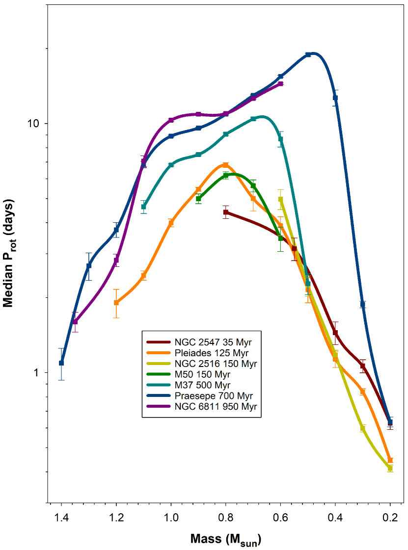
Figure 11 shows, for each cluster in our sample, the period versus mass diagram of the median rotators in $0.1M_{\odot}$ bins. This allows us to simultaneously analyze the mass and age dependence of stellar rotation. For stars with masses below $0.5M_{\odot}$, the median rotation periods for the young NGC 2547 (35 Myr) are longer than those seen in the older Pleiades and NGC 2516 clusters (125 and 150 Myr, respectively). This is consistent with expectations, considering that stars of these masses take a few hundred Myr to reach the ZAMS, and are therefore still contracting by the age of NGC 2547. By the age of Praesepe (700 Myr), these stars have spun down in a strongly mass-dependent fashion, with lowest masses still showing periods below 1 day, and $\sim 0.4M_{\odot}$ stars rotating at $\gtrsim$ 10 days.

The stars more massive than $0.5M_{\odot}$, on the other hand, show a monotonic behavior with time in most of the age range probed by our clusters. They consistently spin down as they age from 35 to 700 Myr, and their median rotator trends in Figure 11 do not intersect each other, in agreement with expectations from a Skumanich-type spin-down (i.e., period $\propto\text{age}^{1/2}$). The notable exception to this, however, is the comparison of Praesepe and NGC 6811. For these two clusters, their rotational sequences do not seem to be simple translations of each other to longer or shorter periods. Although their age difference is non-negligible ($\sim$ 250 Myr), their median rotators are virtually overlapping at $\sim$ 1.1 $M_{\odot}$ and in the $0.8\textendash 0.6M_{\odot}$ range. The latter of these has already been noted by Curtis et al. (2019a) (see also Meibom et al. 2011b), and a similar overlapping was reported by Agüeros et al. (2018) for a smaller sample in the 1.4 Gyr-old cluster NGC 752. In terms of the interpretation of this feature, Agüeros et al. (2018) and Curtis et al. (2019a) have formulated it as a temporary epoch of stalling in the spin-down of K-dwarfs, and Spada & Lanzafame (2020) have proposed that it arises from the competing effect between magnetic braking and a strongly mass-dependent internal redistribution of angular momentum. We leave a detailed examination of this as future work, but given the considerable difference in metallicity between both clusters ([Fe/H]$=+0.16$ dex for Praesepe and $+0.03$ dex for NGC 6811; Netopil et al. 2016), we highlight the importance of incorporating chemical composition in comprehensive models of angular momentum evolution (e.g., Amard & Matt 2020; Amard et al. 2020; Claytor et al. 2020).

Figure 11 can also be used to remark upon global properties of stellar rotation. First, regardless of the age, no sharp transition is seen in the rotation periods near the boundary between partially convective and fully convective stars ($\sim 0.35M_{\odot}$). Second, as illustrated by NGC 2547 in our sample, and by the young Upper Scorpius and Taurus associations in Somers et al. (2017), Rebull et al. (2018), and Rebull et al. (2020), the initial conditions of stellar rotation are strongly mass-dependent, and need to be accounted for in models of angular momentum evolution. Third, when considering the young ages probed by our sample ($\sim$ 35 to 200 Myr), we note that the stars in the $1.0\textendash 0.6M_{\odot}$ range populate a global maximum in terms of rotation periods. In other words, the median rotators in this mass interval never rotate more rapidly than $\sim 3\textendash 4$ days. Given the intimate connection between stellar rotation and activity (e.g., Wright et al. 2011, 2018; Lehtinen et al. 2020), where more rapidly rotating stars tend to expose their planets to higher levels of potentially harmful radiation, this feature could provide an optimal window in the search for habitable worlds.

Figure 12: Distribution of rotation rates as a function of mass for the clusters considered in our sample. The 10th, 25th, 75th and 90th percentiles of the period distributions are computed for 40 star bins in data rank ordered by mass, and then boxcar smoothed. The region of rapid rotators is shown in light grey, that of intermediate rotators is shown in black, and that of slow rotators is shown in dark grey. M50 and NGC 2516 are shown in a combined panel, given their virtually identical ages and complementary mass ranges. We see a clear convergence of rotation rates into a narrow sequence in the older clusters, with the limit (i.e., lowest mass) of this converged branch progressively extending to lower masses for older ages (e.g., $\sim 0.85M_{\odot}$ in the Pleiades to $\sim 0.65M_{\odot}$ in Praesepe). For masses below this, the interquartile range is actually broader in the older clusters than in the younger ones. This suggests that, at fixed mass, the rapid rotators lose less angular momentum (or experience a lower torque) than the slow rotators. Current models of angular momentum evolution do not reproduce this feature.

In Figure 12, we show the rotational sequences for the clusters we study, but in this case separating the data into different percentiles of rotation. For each cluster, across the mass range where they have period information, we show a band of rapid rotators (star within the 10th to 25th percentiles of the period distribution; light grey region), intermediate rotators (25th to 75th percentiles; black region), and slow rotators (75th to 90th percentiles; dark grey region). At young ages, we observe a well-defined upper limit in the rotation periods, with virtually no stars showing periods longer than $\sim$ 10 days. At late ages, we clearly see the convergence of rotation periods to a tight sequence in a heavily mass-dependent fashion, in agreement with expectations. The convergence in our revised sequences is so strong that the upper and lower edges of the distribution in M37, Praesepe, and NGC 6811 in the $1.0\textendash 0.8M_{\odot}$ range are barely visible. Additionally, in both Figures 11 and 12, there is another important clue about the torques from magnetized winds. For all clusters, there is: 1) a characteristic mass where the distribution has collapsed down into a narrow range (the un-saturated domain, where the torque is $\mathrm{d}J/\mathrm{d}t\propto\omega^{3}$); and 2) a mass range just below it where stars still retain a range of surface rotation rates (with the rapid rotators still being in the saturated domain, where the torque is $\mathrm{d}J/\mathrm{d}t\propto\omega$). For this latter mass range, the width of the interquartile range is broader in the older systems ($\gtrsim 500$ Myr) than it is in the young ones ($\lesssim 150$ Myr). This indicates a relative divergence in the surface rotation rates, in contrast to the convergence that is predicted by canonical models of angular momentum loss (e.g., van Saders & Pinsonneault 2013; Matt et al. 2015).

Figure 13: Temporal evolution of the 25th, 50th, and 90th percentiles of the angular velocity distributions (normalized to the solar value). We show this for different masses, with 0.5 $M_{\odot}$ stars shown in the top, 0.8 $M_{\odot}$ stars shown in the middle, and 1 $M_{\odot}$ stars shown in the bottom. Our values are shown as the black solid line (GPR21), and the literature values from Gallet & Bouvier (2015) are shown as the red dashed line (GB15). Our analyses of the clusters’ memberships and properties play a role in shifting our values with respect to the literature ones in both axes (see §6.2).

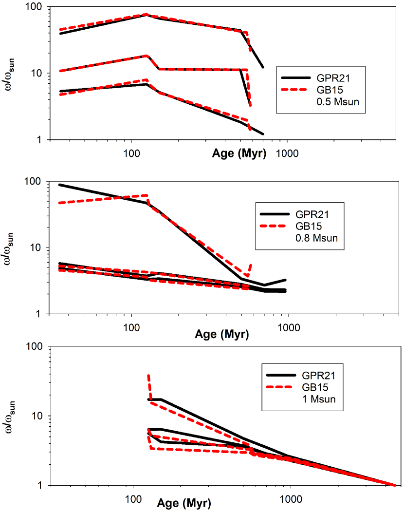
In other words, the data in Figure 12 appear to require lower torques for rapid rotators than for intermediate rotators, which acts to create the bimodal distribution that has been noted in the literature (and which is now clearly seen in our sample). One possible explanation for this, as proposed by Garraffo et al. (2018), is that there is a change in field topology, such that rapid rotators have more complex magnetic field configurations than intermediate rotators, and are therefore less efficient at losing angular momentum. Although this concept is interesting, the data could also be fit with a wind model that incorporates a super-saturation mechanism, where the overall field strength declines. Alternatively, it could indicate a dependence of the convective overturn timescale on the rotation rate at fixed mass, as loss laws are typically parametrized by the ratio of the rotation period to this timescale (i.e., the Rossby number). Ultimately, a number of additional physical properties that are involved in the loss of angular momentum could be influencing the empirical sequences (e.g., mass loss rate, dipole field strength, Alfvén radius). It will be informative to compare different proposed mechanisms, but an adjustment to canonical models is clearly required. We note that the late time behavior of the distribution is not sensitive to the treatment of this feature, as older stars have lost memory of their initial conditions, and typical semi-empirical approaches are tuned to reproduce the spin-down of the slow and rapid rotator branches of the data. However, the properties of intermediate rotators in systems that retain rapid rotators will not be correctly modeled by classical methods.

Finally, in Figure 13, we show the temporal evolution of the rotational percentiles for three different masses ($0.5,0.8$, and $1M_{\odot}$). We frame this as a comparison with Gallet & Bouvier (2015) in terms of the 25th, 50th, and 90th percentiles of the distribution of angular velocities ($\omega=2\pi/P_{\text{rot}}$), normalized to the solar value ($\omega_{\odot}=2.87\times 10^{-6}\text{s}^{-1}$). Our membership analysis plays a role in shifting our values with respect to the literature ones in both axes, as the revised cluster properties change the ages (§4), and the revised rotational sequences change the angular velocity distributions (§5). In general, our percentile evolution appear less noisy and shows smoother patterns. In the $0.5$ and $0.8M_{\odot}$ stars, our data capture the same broad trends. Importantly, the overall slow rotation in young stars remains, and this provides further evidence for the need of core-envelope decoupling in angular momentum models (e.g., Denissenkov et al. 2010). Before our work, the classification of all of the slow rotators in NGC 2547 as field contaminants was a real possibility, and while our analysis did remove a number of them, some still remain. For the $1M_{\odot}$ stars, our data suggests a faster rotation in all percentiles (as our analysis has predominantly removed slow rotators), and a globally steeper spin-down slope that remains approximately constant (and similar to the Skumanich value) in the entire age range.

6.3 Gaia Biases against Photometric Binaries

Figure 14: Period versus temperature (left column), apparent $V$ versus $V-K$ CMD (middle column), and apparent $G$ versus $G_{\text{BP}}-G_{\text{RP}}$ CMD (right column) for the nearby Pleiades (top row) and Praesepe (bottom row) clusters. We take the $V$ and $K$ photometry from Rebull et al. (2016a) and Rebull et al. (2017). The color and symbol coding are the same from the literature sequences of Figure 9. For the purposes of this figure, we highlight the no info stars and non members over the probable members. For both clusters, the stars classified as no info stars appear predominantly as photometric binaries on both CMDs, hinting to biases in the Gaia astrometry for these systems. Notably, while in the $\sim$ 125 Myr Pleiades sequence many no info stars correspond to rapid rotators, almost all of them have converged onto the slowly rotating branch in the $\sim$ 700 Myr Praesepe sequence. This indicates that, although unresolved, these likely binary systems are spinning down as single stars do (see §6.3).

Investigating the behavior of binary stars in empirical rotation studies is important to better understand stellar populations and angular momentum evolution. In the regime of wide separations, binaries can be used to place novel gyrochronology constraints in unexplored age and metallicity domains (Chanamé & Ramírez, 2012; Janes, 2017; Godoy-Rivera & Chanamé, 2018). In the regime of close separations, recent studies have found a correlation between rapid rotation and field binaries (Simonian et al., 2019, 2020). Specifically in the M-dwarf domain, Stauffer et al. (2018) found that in the young Upper Scorpius association ($\sim$ 8 Myr) and the Pleiades cluster, the stars with multiple period measurements from K2 are predominantly photometric binaries (see also Rebull et al. 2016a, Rebull et al. 2017, and Tokovinin & Briceño 2018). Furthermore, Stauffer et al. (2018) showed that the rotation periods of these young, unresolved binaries, are much shorter as well as similar to each other than otherwise expected for single M-dwarfs. This hints at the crucial role that binarity plays in star formation and the rotation rates imprinted at birth (see also Messina 2019).

In this context, in Figure 14 we examine the rotational sequences and CMDs of the no info stars in our most nearby clusters (i.e., the targets that did not pass our astrometric quality cuts; see §3.1.3). In the revised rotational sequences of M50 and M37, the stars classified as no info predominantly occupy their very lowest $T_{\text{eff}}$ (and therefore apparent magnitude) values, which indicates that their classification is purely due to low quality astrometry. In contrast to this, for the Pleiades and Praesepe, the no info stars span the entire $T_{\text{eff}}$ range (see §5), and we would have expected them to have high-quality Gaia astrometry. Considering the previous selections made by Rebull et al. (2016a) in the Pleiades and by Rebull et al. (2017) in Praesepe, and given the low contamination rates found for these systems in §5, we expect most of these no info stars to be real members of these nearby clusters.

The CMDs of Figure 14 show that the no info stars appear, predominantly, as photometric binaries with respect to the sequences of probable members in both the Pleiades and Praesepe. This result hints to biases in the Gaia DR2 data against these unresolved systems, even with conservative quality cuts, where their separation is seemingly too close for the current astrometry to properly distinguish their orbital and systemic motions. Interestingly, many of these no info stars appear as rapid rotators in the Pleiades rotational sequence. By the age of Praesepe, however, they are overlapping with the bulk of the probable members on the slowly rotating branch. This indicates that, while their separations are close enough to be unresolved in Gaia, these binaries are not synchronized and they are actually spinning down in a similar fashion as the single stars do. This finding is similar to that of Stauffer et al. (2018), who reported that the rapid rotation of stars in binaries with respect to single stars is gone by the age of Praesepe, but in this case we extend it to higher mass stars, beyond the M-dwarf regime.

Figure 14 also provides an interesting distinction in our membership classification. While presumably some of the stars classified in the no info category could turn out to be field contaminants, the stars classified as non members appear to occupy different locations in the rotational sequences and CMDs. Most of these non members appear below the track of probable members on the CMD, and correspond to rotational outliers in the converged branch of Praesepe. In addition to their astrometric distinction, we take this as further confirmation that the non members and no info stars correspond to markedly different populations.

Finally, although our astrometric selections were designed to avoid biases against binary stars, we conclude that newer Gaia data will be needed to fully resolve these photometric binaries. In the meanwhile, while not being classified as probable members by our membership analysis, we advise future rotation studies of binary stars to include these no info stars in their samples for completeness purposes.

7 Conclusions

Open clusters have played a key role in stellar rotation studies, but their memberships are often uncertain, and the expected contamination rates can reach up to $\sim$ 60%. In this paper, we use the Gaia DR2 astrometry to revise the memberships of several open clusters with rotational data (Table 1), and provide an updated portrait of stellar rotation as a function of mass, temperature, and age.

For a given cluster, we carry out an unrestricted search for cluster members in the Gaia data by performing astrometric modeling in parallax and proper motion space. From this, we calculate membership probabilities and identify probable cluster members, non members (i.e., field stars), and an intermediate category of possible members (typically faint stars with large astrometric uncertainties). An additional category denominated no info stars is assigned to stars that do not have enough astrometric information to be classified. Although our membership selection only includes astrometric (but not photometric) data, the CMD projections of the probable members show clean isochrone-like sequences for all the clusters (Figure 5).

We use the homogeneous Gaia photometry to derive revised cluster properties (age, distance modulus, reddening; see Table 2) by comparing with state-of-the-art evolutionary models. Importantly, we find our revised ages to be in good agreement with pre Gaia literature estimates, and in some cases, in disagreement with more recent analyses (see §4). We further exploit the Gaia photometry and compare it with models to calculate stellar masses and temperatures for our probable and possible cluster members. All of this allows us to perform an analysis of the clusters’ rotational sequences in a common mass, temperature, and age scale, something that has been missing in previous studies.

We crossmatch the Gaia stars with the rotation period catalogs, and use our membership analysis to remove the non member contaminants from the rotational sequences of the clusters (Figure 9). We find varying degrees of non member contamination, with some of the clusters observed from the ground showing high rates (e.g., $\approx 25\%$ and $36\%$ for NGC 2547 and M50), and the clusters observed from space showing lower rates (e.g., $\approx 4\%$ for the Pleiades). M50 is an exceptional case, where our revised sequence is considerably different from the previous literature one, and its revised sequence now clearly resembles that of the benchmark and similar-age Pleiades cluster.

We present an updated and self-consistent portrait of the evolution of stellar rotation, and quantify important trends that can be obtained from it. Our most important findings in these regards are:

• Once the non member contamination has been removed, the rotational sequences of clusters observed from the ground can be as constraining as those observed from space (Figure 10). This is particularly relevant for the post Kepler and K2 era.

• Although our membership analysis has predominantly removed rotational outliers in all the clusters, many of these still survive at both short and long periods (Figure 10). It is likely that some of these correspond to synchronized binaries (especially the rapid rotators), but most slow rotators appear as typical single stars in astrometric and photometric regards. An alternate explanation for slow rotators would be that there is a small population with very low birth angular momentum. In any case, these stars can no longer be attributed to field contamination and they need to be explained by future theories of angular momentum evolution.

• At young ages, stars in the $1.0\textendash 0.6M_{\odot}$ range populate a global maximum in terms of rotation periods. Given the strong rotation-activity connection in stars, this potentially provides their planets with an optimal window for habitability (Figure 11).

• At the age of the young NGC 2547 cluster ($\sim$ 35 Myr), there is a clear-cut set of maximum periods ($\sim 10$ days), which provides clues about the initial conditions of rotation. At old ages ($\gtrsim 500$ Myr), stars in the $1.1\textendash 0.6M_{\odot}$ rage converge to a sequence that is even narrower than previously observed (Figure 12).

• In the saturated domain, where stars have not yet converged into a uniform sequence at fixed mass, the separation (in terms of rotation periods) between the intermediate and rapid rotators increases with age. This feature is not predicted by classical models, and we interpret it as the latter group experiencing lower torques compared to the former one (Figure 12).

• We find biases in the Gaia data against photometric binaries, which predominantly appear as rapid rotators at young ages, but nonetheless spin-down as single stars do (Figure 14).

The data products of this paper will be a useful reference for the community. For the clusters in our sample, we make publicly available both the catalog of probable and possible members (regardless of whether they have period measurements; Appendix C), as well as the catalog of the periodic stars (regardless of their membership classification; Appendix F). Additionally, we report the percentiles of the rotational distributions as a function of mass and age, which can be used to calibrate future models of angular momentum evolution (Appendix G).

In a broader sense, the field of stellar rotation is entering a new era thanks to the wealth of photometric and astrometric data provided by space-based missions (e.g., Kepler, K2, TESS, and Gaia). As shown in this work, these can be adequately complemented with ground-based observations. Still, although the rotational sequences of numerous star-forming regions, stellar associations, and open clusters exist in the literature, properly accounting for their memberships remains a crucial part of exploiting them in full. Extensions of our work would increase the sample size and take advantage of improved astrometry and RV measurements (e.g., Gaia DR3) to perform full 6D kinematic analyses.

Ultimately, future rotation studies should attempt to answer the several questions that remain open. Besides the ones mentioned in Section §1, some of these include: the importance of shifts in magnetic field topology on the magnetic braking (Metcalfe et al., 2019; Metcalfe & Egeland, 2019); the role that bright faculae play in stellar variability (e.g., Montet et al. 2017; Reinhold & Hekker 2020); and the deep connection between rotation and the various aspects of stellar activity (e.g., Stelzer et al. 2013; Zhang et al. 2020; Dixon et al. 2020; Godoy-Rivera et al. 2021; Ilin et al. 2021).

Appendix A Potential Expansions to our Cluster Sample

There are a number of systems that we initially considered including in our sample given their high scientific interest, but that we discarded for specific reasons, which we discuss below. We leave an equivalent investigation of them as future work to be done with a more sophisticated underlying model, and when higher precision astrometry becomes available.

• $\rho$ Ophiuchus, Taurus, Upper Scorpius, and h Per: Rebull et al. (2018), Rebull et al. (2020), and Moraux et al. (2013) reported periods for these young associations (ages of $\sim$ 1, 3, 8, and 13 Myr, respectively). Given their young ages, these systems offer interesting pre main-sequence stellar rotation constraints. For the first three of these, however, their more complex kinematics and reddening distributions would likely require somewhat different analysis techniques. For h Per, on the other hand, its small parallax ($\approx$ 0.399 mas; Cantat-Gaudin et al. 2018) and the current precision of the faint star Gaia data precludes a thorough examination. Therefore, we defer the consideration of these systems to a subsequent paper.

• IC 2391/2602 and $\alpha$ Per: with ages of $\sim$ 50 and $\sim$ 80 Myr respectively, these clusters offer snapshots of the evolution of stellar rotation at young ages that could be compared with slightly younger and older systems (e.g., NGC 2547 and the Pleiades). Unfortunately, the rotation samples for these systems are still small ($<$ 40 stars each) and heterogeneous (Denissenkov et al., 2010; Gallet & Bouvier, 2015).

• M34: rotation periods for stars in this $\sim$ 220 Myr-old cluster have been reported by Irwin et al. (2006) (as one of the Monitor Project targets), James et al. (2010), and Meibom et al. (2011a). Although we initially attempted to include M34 in our sample, the Gaia data of this system showed odd gaps in spatial and magnitude space, possibly related to problems with the scanning pattern of this region of the sky. This prevented us from carrying out a similar study for this cluster at this time.

• Hyades: rotation periods for stars in this $\sim$ 625 Myr-old cluster have been reported by a number of authors (e.g., Delorme et al. 2011, Douglas et al. 2016, Douglas et al. 2019), and the Hyades is sufficiently close ($\approx$ 47 pc; Gaia Collaboration et al. 2018b) and well studied that we do not anticipate substantial membership issues.

• NGC 6819: rotation periods for 30 stars in this cluster were reported by Meibom et al. (2015). Given its age of $\sim$ 2 Gyr (Bossini et al., 2019), studying this cluster is of high scientific interest. However, given its small parallax ($\approx$ 0.356 mas; Cantat-Gaudin et al. 2018), and the current precision of the Gaia data, this cluster would naturally be harder to fit with our current method.

Appendix B Astrometric Cluster Parameters and Comparison with the Literature

Figure 15: Comparison of our cluster parameters with literature reference values from Cantat-Gaudin et al. (2018) and Gaia Collaboration et al. (2018b). Left Panel: Parallax difference divided by our parallax value, as a function of our parallax value. The comparison with Cantat-Gaudin et al. (2018) is shown as the filled squares, while the comparison with Gaia Collaboration et al. (2018b) is shown as the open circles. Each of the seven clusters we study is plotted with a different color, and this is indicated by the appropriate text near the bottom. The black dashed line shows a $\pm$ 2% fractional difference for reference. To make an accurate parallax comparison, we are adding the same zero-point value to the parallax of all three sources. Middle and Right Panels: same as the left panel for $\mu_{\alpha}$ and $\mu_{\delta}$. Note that Gaia Collaboration et al. (2018b) do not report cluster parameters for M37 and NGC 6811.

Table 3: Astrometric cluster parameters.

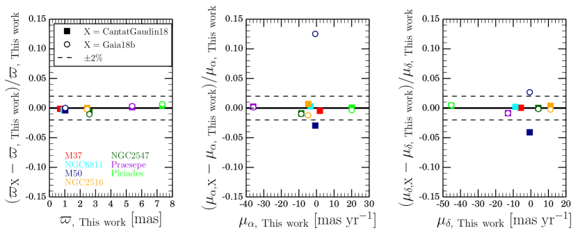
Cluster Name	$\varpi$	$\sigma_{\varpi}$	$\mu_{\alpha}$	$\sigma_{\mu_{\alpha}}$	$\mu_{\delta}$	$\sigma_{\mu_{\delta}}$
-	[mas]	[mas]	[mas yr-1]	[mas yr-1]	[mas yr-1]	[mas yr-1]
NGC 2547	2.600	0.072	-8.686	0.550	4.261	0.457
Pleiades	7.344	0.269	20.066	1.505	-45.325	2.312
M50	1.030	0.023	-0.709	0.257	-0.637	0.170
NGC 2516	2.446	0.065	-4.716	0.592	11.179	0.484
M37	0.696	0.031	1.933	0.184	-5.645	0.171
Praesepe	5.382	0.120	-36.001	1.171	-13.031	0.967
NGC 6811	0.926	0.018	-3.389	0.120	-8.794	0.122

Using the method described in §3.1, we calculate the astrometric parameters for the seven clusters we study. These values are reported in Table 3. We compare our cluster parameters with those reported by Cantat-Gaudin et al. (2018) and Gaia Collaboration et al. (2018b) in Figure 15.

We find an excellent agreement with the literature, with most of the fractional differences being less than $\pm$ 2%. The only exceptions to this are the proper motion parameters of M50 (dark blue points in Figure 15). This is perhaps not surprising, as the M50 proper motion in both coordinates is quite small (and similar to that of the field). We would therefore naturally expect this system to show the largest differences. We nonetheless note that Cantat-Gaudin et al. (2018) and Gaia Collaboration et al. (2018b) also get the largest disagreements between their values for M50, and our parameters are in between their values.

Appendix C Data Table for the Probable and Possible Cluster Members

Table 4 lists the probable and possible cluster members for all the clusters we study. We report the main Gaia DR2 astrometric and photometric information, as well as the membership parameters and classifications we derive.

We caution that, while Table 4 reports the same set of values for all stars regardless their membership classification, the $M_{G_{0,\text{proj}}}$, mass, and $T_{\text{eff}}$ values are calculated assuming as if all the stars are true main-sequence cluster members (and are all at the same respective global cluster parallax). For stars that turn out not to be real members, this will naturally yield an incorrect mass and $T_{\text{eff}}$ estimate. Therefore, we suggest that interested readers should only consider the mass and $T_{\text{eff}}$ values for the probable members as being meaningful in future studies, until higher quality astrometry fully resolves the membership classification of the possible members here reported.

Table 4: Main information and properties for the probable and possible cluster members.

Column	Source	Description
Cluster	This paper	Cluster with respect to which this star’s membership was calculated
Gaia DR2	Gaia DR2 Catalog	Gaia DR2 Source ID
$\alpha$	Gaia DR2 Catalog	RA coordinate
$\delta$	Gaia DR2 Catalog	Dec coordinate
$\varpi$	Gaia DR2 Catalog	Parallax (not including zero-point value)
$\sigma_{\varpi}$	Gaia DR2 Catalog	Parallax error
$\mu_{\alpha}$	Gaia DR2 Catalog	Proper motion in RA
$\sigma_{\mu_{\alpha}}$	Gaia DR2 Catalog	Proper motion in RA error
$\mu_{\delta}$	Gaia DR2 Catalog	Proper motion in Dec
$\sigma_{\mu_{\delta}}$	Gaia DR2 Catalog	Proper motion in Dec error
$G$	Gaia DR2 Catalog	$G$ band magnitude
$G_{\text{BP}}$	Gaia DR2 Catalog	$G_{\text{BP}}$ band magnitude
$G_{\text{RP}}$	Gaia DR2 Catalog	$G_{\text{RP}}$ band magnitude
$G_{\text{BP}}-G_{\text{RP}}$	Gaia DR2 Catalog	$G_{\text{BP}}-G_{\text{RP}}$ color
$\Delta$	This paper	$\Delta$ quantity (as defined in Equation (6))
Probability	This paper	Membership probability (as defined in Equation (7))
Classification	This paper	Membership classification (i.e., probable or possible member)
$M_{G_{0,\text{proj}}}$	This paper	Projected absolute and dereddened $G$ band magnitude
Mass	This paper	Mass obtained by interpolating the best-fit cluster model
$T_{\text{eff}}$	This paper	Effective temperature obtained by interpolating the best-fit cluster model
Flag Mass & $T_{\text{eff}}$	This paper	Regime in which the $M_{G_{0,\text{proj}}}$, mass, and $T_{\text{eff}}$ values were calculated

Appendix D Astrometric Analysis of Clusters and Phase-Space Projections

After applying our classification method to all the clusters, we obtain a sample of probable members, possible members, non members, and no info stars for each of them. Figure 16 shows the phase-space projections of these populations (except for the no info stars, which are absent from the plot due to the lack of astrometric information; see §3.1.3). We now provide an analysis of the astrometric classification in each of the clusters:

Figure 16: Phase-space projections of the probable (blue), possible (cyan), and non (red) members for all the clusters we study (analogous to Figure 2). Each cluster corresponds to a row, and they are sorted as presented in Table 1. Note that the range of the parallax and proper motions vary considerably on a cluster by cluster basis.

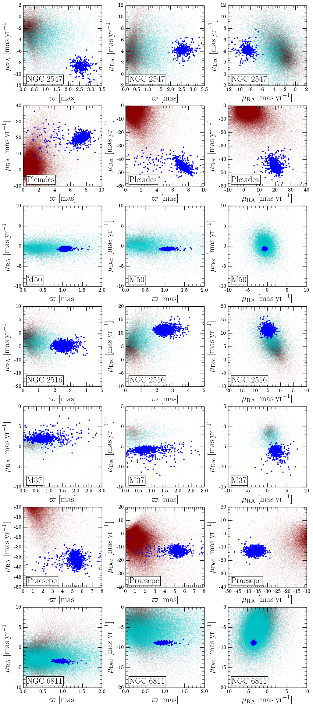
• NGC 2547: for this cluster, the parallax and proper motion in RA are the variables that allow us to distinguish the cluster from the field population in phase-space. On the other hand, the proper motion in Dec of the cluster is similar to that of the field. The possible members are an intermediate population located in between the cluster and the field in the phase-space projections.

• Pleiades: of all the clusters in our sample, this cluster is the one that is the most separated from the field in phase-space. Given its large parallax, as well as proper motion (particularly in Dec), this cluster can be readily differentiated from the background population. Some of the probable members appear as outliers in the projections including parallax, but they correspond to faint stars (apparent $G\gtrsim$ 18.5 mag) with uncertain parallax measurements. The small number of stars classified as possible members is a direct consequence of the large kinematic differences between the cluster and the field. In other words, it is unlikely that a star will have a value of $\Delta_{i}\leq 3$ (inside the cluster’s 3$\sigma$ ellipsoid in phase-space) and will have a low cluster membership probability.

• M50: in this case, the proper motion of the cluster is quite similar to that of the field, and therefore the parallax plays a crucial role in identifying the probable cluster members. Nonetheless, given the small cluster parallax ($\sim$ 1.0 mas) and the therefore larger astrometric uncertainties associated (as the stars in M50 are naturally fainter than those of, for instance, the Pleiades), together with the proper motion similarities with the field, the number of possible members for this cluster is much larger than for others. In other words, given the large astrometric uncertainties, there are a large number of stars with values of $\Delta_{i}\leq 3$ (inside the cluster’s 3$\sigma$ ellipsoid) that have low membership probabilities ($P<P_{\text{min}}$). The CMD of this cluster (see Figure 5) demonstrates this, as for magnitudes fainter than apparent $G\simeq 17$ mag, the probable members are surrounded by an envelope of possible members. Additionally, the proper motion projection shows that the possible members are overlapping with the non members altogether.

• NGC 2516: for this cluster, the parallax plays an important role when identifying the probable members. Although there are differences between the cluster and field proper motions (more in the Dec coordinate than in RA), the parallax is the dominant means to separate the populations. As in the case of NGC 2547, the possible members appear as an intermediate population in the phase-space projections.

• M37: this cluster has the smallest parallax of our entire sample, in addition to having a proper motion in RA rather similar to that of the field. Thus, the proper motion in Dec plays an important role in the astrometric classification. M37 is also the richest cluster in our sample, and we identify a large number of probable members that densely populate the CMD. Moreover, a few giant stars can be seen in the CMD, highlighting that our classification method is agnostic to the stars photometry, and they naturally arise from a careful astrometric selection. Similarly as for the Pleiades, the probable members that appear as phase-space outliers correspond to faint stars.

• Praesepe: similarly to the Pleiades, this cluster is clearly separated from the field in phase-space. Again, some of the probable members appear as outliers particularly in proper motion space, but they correspond to faint stars with large astrometric uncertainties. The small number of possible members is again a reflection of the large kinematic difference between the cluster and field.

• NGC 6811: this cluster has a similar proper motion in RA to that of the field, and therefore the parallax and proper motion in Dec are the variables that allow us to better distinguish the probable cluster members from the non members. However, given its small parallax value (compared to other clusters), and similarly to M50, NGC 6811 also has a large number of stars classified as possible members that overlap with the non members in phase-space (and moreover, for magnitudes fainter than apparent $G\simeq$ 19 mag, the astrometric errors are so large that no star can be reliably classified as a probable member).

Appendix E Comparison of our Masses and Temperatures with Literature values

Figure 17: Comparison of our mass and $T_{\text{eff}}$ estimates with literature values (analogous to Figure 7). The mass comparisons are shown in yellow, while the $T_{\text{eff}}$ comparisons are shown in purple. The axis scale is the same for all the mass and $T_{\text{eff}}$ comparisons. Each panel indicates the respective cluster name in the top right corner and the mean and standard deviation of the mass or $T_{\text{eff}}$ difference in the bottom right corner. The dotted and dashed lines correspond to the apparent $G=17.5$ and 18.5 mag limits from Figure 5 translated to mass and $T_{\text{eff}}$ coordinates. The comparisons suggest that our masses and temperatures are subject to systematic uncertainties of $\sim 0.05\textendash 0.1M_{\odot}$ and $\sim 150$ K, which are modest considering the different methods, photometric data, and underlying models employed.

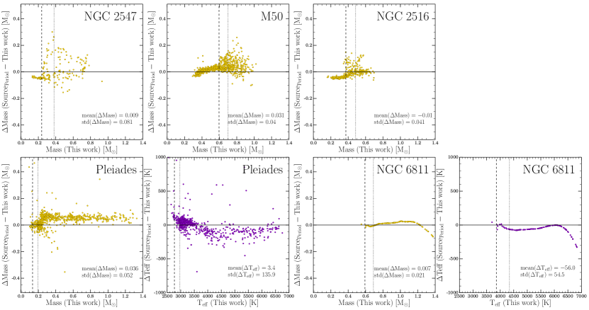
Analogous to the comparison made in §4.2 for NGC 2547, some of the other clusters we study have mass (and sometimes $T_{\text{eff}}$) estimates available in the references that we use as sources for the period information. In particular, Irwin et al. (2008), Irwin et al. (2009), and Irwin et al. (2007a) report masses for the NGC 2547, M50, and NGC 2516 stars, and Stauffer et al. (2016) and Curtis et al. (2019a) report mass and $T_{\text{eff}}$ for the Pleiades and NGC 6811 stars. We show the comparison of these estimates with ours in Figure 17. Note that for M37 and Praesepe the references used as sources for the period information did not report mass or temperature estimates, and these clusters are missing from the comparison.

The mass comparisons with NGC 2547, M50, and NGC 2516 are topologically similar to each other: in the faint regime (masses below the dashed lines), where we do not account for the contribution of photometric binaries, we see mostly constant differences of order $\approx-0.05M_{\odot}$. For masses higher than this limit, the scatter increases and we observe that many stars have positive mass differences, which is due to the magnitude projections we use in the intermediate and bright regimes.

For the Pleiades, the mass and temperature comparisons with Stauffer et al. (2016) are in agreement with our expectations: while we employed the projection technique to account for unresolved binaries in our bright regime and partially in our intermediate regime, Stauffer et al. (2016) used this approach for their entire sample. Accordingly, we observe an approximately constant offset trend in $\Delta$Mass ($\approx+0.05M_{\odot}$) and $\Delta T_{\text{eff}}$ ($\approx-150$ K) for stars more massive/hotter than the dotted line, which then turns to a mass/$T_{\text{eff}}$-dependent trend for stars in the intermediate and faint regimes.

For NGC 6811, Curtis et al. (2019a) derived temperatures by generating their own color-$T_{\text{eff}}$ relations, and translated these to masses by interpolating tabulated spectral energy distributions. The mass and $T_{\text{eff}}$ comparisons show an excellent agreement, with differences being $\lesssim 0.025M_{\odot}$ and $\lesssim 100$ K for most of the mass/$T_{\text{eff}}$ range. Given that both our and their calculations are based only on the Gaia DR2 photometry (unlike the previously described comparisons), this result is consistent with the expectations.

Ultimately, all the mass and temperature comparisons previously described are subject to different assumptions regarding the cluster properties, stellar evolutionary models (and their specific input physics; e.g., Tayar et al. 2020), and considerations for the contribution of unresolved photometric binaries. Furthermore, in most cases, the photometry employed by the references that supply the period information is different from that of Gaia. In spite of this, we observe a good overall agreement with the literature estimates, and these comparisons suggest possible systematic uncertainties of $\sim 0.05\textendash 0.1M_{\odot}$ and $\sim 150$ K in our masses and temperatures.

Appendix F Data Table for the Periodic Samples

Table 5 reports the main information and properties for the periodic samples of the clusters we study. We list all stars that were reported in the catalogs used as sources for the periods (see §2), regardless of their membership classification, or if we found them when crossmatching with the Gaia DR2 data. We extend the same cautionary note given in Table 4 to Table 5, regarding that the $M_{G_{0,\text{proj}}}$, mass, and $T_{\text{eff}}$ values are calculated assuming as if all the stars are true main-sequence cluster members (and are all at the same respective global cluster parallax).

Table 5: Main information and properties for the periodic samples.

Column	Source	Description
Cluster	This paper	Cluster with respect to which this star’s membership was calculated
Source ID	Period Source Catalog	ID in the catalog used as source of the period information
Period	Period Source Catalog	Period
Gaia DR2	Gaia DR2 Catalog	Gaia DR2 Source ID
$\alpha$	Gaia DR2 Catalog	RA coordinate
$\delta$	Gaia DR2 Catalog	Dec coordinate
$\varpi$	Gaia DR2 Catalog	Parallax (not including zero-point value)
$\sigma_{\varpi}$	Gaia DR2 Catalog	Parallax error
$\mu_{\alpha}$	Gaia DR2 Catalog	Proper motion in RA
$\sigma_{\mu_{\alpha}}$	Gaia DR2 Catalog	Proper motion in RA error
$\mu_{\delta}$	Gaia DR2 Catalog	Proper motion in Dec
$\sigma_{\mu_{\delta}}$	Gaia DR2 Catalog	Proper motion in Dec error
$G$	Gaia DR2 Catalog	$G$ band magnitude
$G_{\text{BP}}$	Gaia DR2 Catalog	$G_{\text{BP}}$ band magnitude
$G_{\text{RP}}$	Gaia DR2 Catalog	$G_{\text{RP}}$ band magnitude
$G_{\text{BP}}-G_{\text{RP}}$	Gaia DR2 Catalog	$G_{\text{BP}}-G_{\text{RP}}$ color
$\Delta$	This paper	$\Delta$ quantity (as defined in Equation (6))
Probability	This paper	Membership probability (as defined in Equation (7))
Classification	This paper	Membership classification
$M_{G_{0,\text{proj}}}$	This paper	Projected absolute and dereddened $G$ band magnitude
Mass	This paper	Mass obtained by interpolating the best-fit cluster model
$T_{\text{eff}}$	This paper	Effective temperature obtained by interpolating the best-fit cluster model
Flag Mass & $T_{\text{eff}}$	This paper	Regime in which the $M_{G_{0,\text{proj}}}$, mass, and $T_{\text{eff}}$ values were calculated

Appendix G Percentiles of the Period Distributions

Table 6 reports the percentiles of the distribution of rotation periods as a function of mass and age. Note that only the stars that survive our membership analysis have been considered (i.e., the stars of the revised rotational sequences, see Figure 10). These values can be used to calibrate and test future models of angular momentum evolution.

Table 6: Percentiles of the distribution of rotation periods as a function of mass and age.

Cluster	Age	Mass	N⋆	$\text{P}_{10}$	MAD10	$\sigma_{10}$	$\text{P}_{25}$	MAD25	$\sigma_{25}$	$\text{P}_{50}$	MAD50	$\sigma_{50}$	$\text{P}_{75}$	MAD75	$\sigma_{75}$	$\text{P}_{90}$	MAD90	$\sigma_{90}$
-	[Myr]	[$M_{\odot}$]	-	[days]	[days]	[days]	[days]	[days]	[days]	[days]	[days]	[days]	[days]	[days]	[days]	[days]	[days]	[days]
NGC 2547	35	0.2	34	0.318	0.091	0.035	0.471	0.101	0.024	0.628	0.212	0.036	0.886	0.13	0.032	1.161	0.218	0.084
NGC 2547	35	0.3	29	0.393	0.04	0.017	0.586	0.193	0.051	1.063	0.344	0.064	1.369	0.161	0.042	2.408	0.81	0.336
NGC 2547	35	0.4	24	0.39	0.152	0.069	0.78	0.317	0.092	1.447	0.747	0.152	5.024	2.873	0.829	8.045	0.747	0.341
NGC 2547	35	0.55	24	0.807	0.409	0.187	1.591	0.433	0.125	3.146	1.61	0.329	5.111	1.463	0.422	7.287	1.43	0.652
NGC 2547	35	0.8	21	0.287	0.06	0.029	1.219	0.922	0.285	4.41	1.197	0.261	5.221	0.268	0.083	5.56	0.192	0.094
Pleiades	125	0.2	268	0.238	0.041	0.006	0.308	0.051	0.004	0.445	0.148	0.009	0.653	0.134	0.012	0.909	0.161	0.022
Pleiades	125	0.3	132	0.457	0.068	0.013	0.611	0.139	0.017	0.837	0.283	0.025	1.241	0.322	0.04	2.011	0.262	0.051
Pleiades	125	0.4	70	0.288	0.032	0.009	0.476	0.207	0.035	1.134	0.709	0.085	1.996	0.462	0.078	4.041	1.584	0.423
Pleiades	125	0.5	40	0.327	0.022	0.008	0.597	0.277	0.062	2.153	1.56	0.247	3.734	1.333	0.298	7.434	0.674	0.238
Pleiades	125	0.6	54	0.399	0.094	0.029	1.661	1.304	0.251	3.887	2.48	0.337	6.641	1.83	0.352	9.292	0.667	0.203
Pleiades	125	0.7	35	0.394	0.048	0.018	0.56	0.199	0.047	5.002	3.235	0.547	7.479	0.889	0.212	8.44	0.158	0.06
Pleiades	125	0.8	23	0.54	0.226	0.105	6.13	0.627	0.185	6.813	0.742	0.155	7.65	0.336	0.099	8.249	0.302	0.141
Pleiades	125	0.9	28	0.831	0.142	0.06	4.031	1.374	0.367	5.444	0.548	0.103	5.933	0.22	0.059	6.154	0.005	0.002
Pleiades	125	1	20	1.476	0.765	0.382	3.297	0.211	0.067	3.991	0.658	0.147	4.549	0.465	0.147	5.137	0.575	0.287
Pleiades	125	1.1	18	1.116	0.279	0.147	2.138	0.259	0.086	2.453	0.455	0.107	3.081	0.552	0.184	3.907	0.334	0.176
Pleiades	125	1.2	14	0.856	0.026	0.016	1.172	0.334	0.126	1.908	0.933	0.249	3.095	0.952	0.36	6.792	0.07	0.042
NGC 2516	150	0.2	27	0.291	0.038	0.017	0.37	0.027	0.007	0.413	0.068	0.013	0.561	0.101	0.027	2.136	1.487	0.64
NGC 2516	150	0.3	86	0.34	0.029	0.007	0.46	0.09	0.014	0.599	0.185	0.02	0.829	0.181	0.028	1.194	0.169	0.041
NGC 2516	150	0.4	110	0.364	0.056	0.012	0.605	0.236	0.032	1.179	0.541	0.052	1.685	0.414	0.056	2.987	0.709	0.151
NGC 2516	150	0.5	72	0.334	0.052	0.014	0.558	0.257	0.043	2.235	1.759	0.207	4.879	1.853	0.309	6.694	0.974	0.257
NGC 2516	150	0.6	49	0.446	0.039	0.012	1.282	0.95	0.192	4.971	3.227	0.461	7.756	1.268	0.256	9.606	0.908	0.29
M50	150	0.6	54	0.272	0.024	0.007	0.53	0.3	0.058	3.452	2.828	0.385	6.417	1.754	0.338	10.327	2.364	0.719
M50	150	0.7	106	0.456	0.111	0.024	1.116	0.844	0.116	5.627	3.191	0.31	7.753	1.104	0.152	9.522	0.666	0.145
M50	150	0.8	57	0.723	0.161	0.048	3.48	1.941	0.363	6.188	1.594	0.211	7.47	0.481	0.09	8.483	0.651	0.193
M50	150	0.9	46	1.29	0.854	0.282	3.633	1.137	0.237	4.992	1.541	0.227	6.723	0.923	0.192	7.868	0.626	0.206
M37	500	0.5	67	0.579	0.063	0.017	0.779	0.316	0.055	2.273	1.782	0.218	13.758	3.185	0.55	16.609	0.857	0.234
M37	500	0.6	78	1.292	0.352	0.089	2.208	1.073	0.172	8.665	5.491	0.622	13.801	1.147	0.184	15.055	0.473	0.12
M37	500	0.7	63	5.134	0.775	0.218	7.418	2.248	0.4	10.435	1.211	0.153	11.474	0.601	0.107	12.388	0.23	0.065
M37	500	0.8	58	7.512	0.401	0.118	8.242	0.429	0.08	9.06	0.821	0.108	9.902	0.377	0.07	10.303	0.189	0.056
M37	500	0.9	39	6.829	0.168	0.06	7.162	0.178	0.04	7.507	0.51	0.082	8.249	0.486	0.11	9.731	1.246	0.446
M37	500	1	18	5.372	0.356	0.188	6.37	0.354	0.118	6.817	0.272	0.064	7.01	0.175	0.058	8.514	1.166	0.615
M37	500	1.1	18	3.225	0.049	0.026	3.531	0.383	0.128	4.632	1.182	0.279	6.22	0.609	0.203	6.776	0.46	0.243
Praesepe	700	0.2	132	0.254	0.026	0.005	0.331	0.09	0.011	0.635	0.331	0.029	1.138	0.364	0.045	1.806	0.194	0.038
Praesepe	700	0.3	186	0.858	0.251	0.041	1.268	0.25	0.026	1.878	0.779	0.057	5.09	2.958	0.307	16.447	3.984	0.653
Praesepe	700	0.4	86	0.902	0.122	0.029	3.25	2.352	0.359	12.682	8.758	0.944	20.605	4.221	0.644	25.071	1.267	0.306
Praesepe	700	0.5	53	2.076	1.037	0.319	16.739	2.013	0.391	18.873	2.064	0.283	20.857	1.141	0.222	23.111	1.049	0.322
Praesepe	700	0.6	63	7.529	3.363	0.948	14.365	0.846	0.151	15.454	1.133	0.143	16.732	0.682	0.121	18.07	0.645	0.182
Praesepe	700	0.7	55	11.743	0.174	0.053	12.199	0.384	0.073	12.969	0.667	0.09	13.607	0.371	0.071	14.511	0.27	0.081
Praesepe	700	0.8	29	9.368	0.807	0.335	10.421	0.249	0.066	10.886	0.552	0.103	11.556	0.26	0.068	12.073	0.257	0.107
Praesepe	700	0.9	34	8.059	0.259	0.099	9.147	0.239	0.058	9.585	0.424	0.073	10.049	0.393	0.095	11.816	0.903	0.346
Praesepe	700	1	30	4.489	1.513	0.618	8.048	0.557	0.144	8.899	0.472	0.086	9.088	0.107	0.028	10.268	0.642	0.262
Praesepe	700	1.1	22	4.399	0.336	0.16	5.928	0.826	0.249	6.845	0.923	0.197	7.897	0.334	0.101	8.548	0.561	0.267
Praesepe	700	1.2	14	—	—	—	3.122	0.497	0.188	3.745	0.969	0.259	5.077	0.443	0.168	—	—	—
Praesepe	700	1.3	12	—	—	—	1.008	0.282	0.115	2.686	1.178	0.34	3.657	0.377	0.154	—	—	—
Praesepe	700	1.4	8	—	—	—	0.71	0.214	0.107	1.092	0.452	0.16	1.919	0.565	0.283	—	—	—
NGC 6811	950	0.6	12	—	—	—	13.983	0.403	0.164	14.43	0.375	0.108	14.97	0.54	0.22	—	—	—
NGC 6811	950	0.7	51	11.48	0.233	0.073	11.917	0.175	0.035	12.597	0.679	0.095	13.203	0.422	0.084	15.841	2.391	0.749
NGC 6811	950	0.8	36	7.82	2.626	0.978	10.591	0.256	0.06	10.966	0.447	0.074	11.672	0.705	0.166	12.859	0.349	0.13
NGC 6811	950	0.9	35	9.747	0.136	0.051	10.47	0.345	0.082	10.89	0.371	0.063	11.26	0.369	0.088	12.376	0.623	0.235
NGC 6811	950	1	25	9.555	0.009	0.004	9.918	0.305	0.086	10.303	0.588	0.118	10.929	0.482	0.136	13.007	0.253	0.113
NGC 6811	950	1.1	26	4.785	0.518	0.227	6.204	0.689	0.191	7.066	1.834	0.36	9.35	0.602	0.167	10.842	0.889	0.39
NGC 6811	950	1.2	26	1.472	0.122	0.054	2.022	0.278	0.077	2.828	0.824	0.162	3.726	0.763	0.212	7.434	2.693	1.181
NGC 6811	950	1.35	14	—	—	—	0.987	0.067	0.025	1.601	0.547	0.146	2.145	0.199	0.075	—	—	—

Note. — The clusters are sorted by increasing age. The quoted ages come from the compilation by Gallet & Bouvier (2015) and are the representative pre Gaia values. The period measurements are taken from the references cited throughout §2.

Note. — Summary of the revised and updated cluster properties (age, metallicity, distance modulus, and reddening) that we adopt to calculate masses and temperatures, as well as in our discussion throughout §6. The cluster distances are also shown for reference. We calculate distance moduli from our astrometric analysis, survey the literature for updated high-resolution spectroscopic metallicity measurements, and estimate reddening and age from a CMD analysis of the probable cluster members.

Note. — List of cluster parameters (parallax, proper motion in $\alpha$ and $\delta$, and their respective dispersions) for the seven clusters we study. These are the values we use in Equation (7) to calculate membership probabilities. Note that the reported parallax values include the global 29 $\mu$as zero-point offset described in §3.1.1, with the exception of NGC 6811, for which we use the Kepler field 53 $\mu$as zero-point value from Zinn et al. (2019).

Note. — (The full table is available online in machine-readable format.) We report the main Gaia DR2 astrometric and photometric information, as well as the membership parameters we calculate, for the stars we classify as probable and possible cluster members. We also report our derived projected absolute and dereddened $G$ band magnitudes ($M_{G_{0,\text{proj}}}$), as well as the respective mass and temperature values obtained by interpolating the models, and the regime in which they were calculated (see §4.2 for details). The parallaxes are reported as they appear in Gaia DR2 and do not include the zero-point values we have used elsewhere. For abbreviation purposes we only list the possible members with membership probabilities greater than 50%. We are glad to provide extended tables (including the same information for all the possible members as well as for the non members and no info stars) to interested readers upon request.

Note. — (The full table is available online in machine-readable format.) From the catalogs used as source of the period measurements, we report the IDs used in them (which vary on a cluster by cluster basis) and the periods. We note that although many of the Pleiades and Praesepe stars had more than one period reported, this table only lists their main value, i.e., $P1$ from Rebull et al. (2016a, b) and Rebull et al. (2017), respectively. From Gaia DR2, we report the main astrometric and photometric information, and the parallaxes are reported as they appear in Gaia DR2 and do not include the zero-point values we have used elsewhere. From our analysis we report the membership probability and classification regardless of their category (i.e., probable, possible or non member, or no info star). We also report our derived projected absolute and dereddened $G$ band magnitudes ($M_{G_{0,\text{proj}}}$), as well as the respective mass and temperature values obtained by interpolating the models, and the regime in which they were calculated (see §4.2 for details).

Note. — (The table is also available online in machine-readable format.) The clusters are sorted by their revised age values, and only the stars that survive our membership analysis are considered. The data are binned in $0.1M_{\odot}$ bins (unless otherwise indicated), then rank ordered from short to long periods. For each cluster, we report the 10th, 25th, 50th, 75th, and 90th percentiles in the period distribution, along with their median absolute deviations (MAD). Standard errors of the medians are converted from MADs using the assumption of a normal distribution and root N statistics. The 10th and 90th percentiles are not presented for bins with less than 20 entries. The 0.55 and 0.8 $M_{\odot}$ bins for NGC 2547 and the 1.35 $M_{\odot}$ bin for NGC 6811 are binned in broader bins ($0.45\textendash 0.70$, $0.7\textendash 0.9$, and $1.25\textendash 1.45M_{\odot}$, respectively) because of small sample sizes.

References

- Agüeros et al. (2011) Agüeros, M. A., Covey, K. R., Lemonias, J. J., et al. 2011, ApJ, 740, 110, doi: 10.1088/0004-637X/740/2/110
- Agüeros et al. (2018) Agüeros, M. A., Bowsher, E. C., Bochanski, J. J., et al. 2018, ApJ, 862, 33, doi: 10.3847/1538-4357/aac6ed
- Amard & Matt (2020) Amard, L., & Matt, S. P. 2020, ApJ, 889, 108, doi: 10.3847/1538-4357/ab6173
- Amard et al. (2020) Amard, L., Roquette, J., & Matt, S. P. 2020, MNRAS, 499, 3481, doi: 10.1093/mnras/staa3038
- Anderson et al. (1966) Anderson, C. M., Stoeckly, R., & Kraft, R. P. 1966, ApJ, 143, 299, doi: 10.1086/148512
- Angus et al. (2015) Angus, R., Aigrain, S., Foreman-Mackey, D., & McQuillan, A. 2015, MNRAS, 450, 1787, doi: 10.1093/mnras/stv423
- Angus et al. (2019) Angus, R., Morton, T. D., Foreman-Mackey, D., et al. 2019, AJ, 158, 173, doi: 10.3847/1538-3881/ab3c53
- Angus et al. (2020) Angus, R., Beane, A., Price-Whelan, A. M., et al. 2020, AJ, 160, 90, doi: 10.3847/1538-3881/ab91b2
- Arenou et al. (2018) Arenou, F., Luri, X., Babusiaux, C., et al. 2018, A&A, 616, A17, doi: 10.1051/0004-6361/201833234
- Baraffe et al. (1998) Baraffe, I., Chabrier, G., Allard, F., & Hauschildt, P. H. 1998, A&A, 337, 403. https://arxiv.org/abs/astro-ph/9805009
- Baraffe et al. (2015) Baraffe, I., Homeier, D., Allard, F., & Chabrier, G. 2015, A&A, 577, A42, doi: 10.1051/0004-6361/201425481
- Barnes (2003) Barnes, S. A. 2003, ApJ, 586, L145, doi: 10.1086/374681
- Barnes (2007) —. 2007, ApJ, 669, 1167, doi: 10.1086/519295
- Belokurov et al. (2020) Belokurov, V., Penoyre, Z., Oh, S., et al. 2020, MNRAS, 496, 1922, doi: 10.1093/mnras/staa1522
- Borucki et al. (2010) Borucki, W. J., Koch, D., Basri, G., et al. 2010, Science, 327, 977, doi: 10.1126/science.1185402
- Bossini et al. (2019) Bossini, D., Vallenari, A., Bragaglia, A., et al. 2019, A&A, 623, A108, doi: 10.1051/0004-6361/201834693
- Bouma et al. (2021) Bouma, L. G., Curtis, J. L., Hartman, J. D., Winn, J. N., & Bakos, G. Á. 2021, arXiv e-prints, arXiv:2107.08050. https://arxiv.org/abs/2107.08050
- Bressan et al. (2012) Bressan, A., Marigo, P., Girardi, L., et al. 2012, MNRAS, 427, 127, doi: 10.1111/j.1365-2966.2012.21948.x
- Cantat-Gaudin et al. (2018) Cantat-Gaudin, T., Jordi, C., Vallenari, A., et al. 2018, A&A, 618, A93, doi: 10.1051/0004-6361/201833476
- Cardelli et al. (1989) Cardelli, J. A., Clayton, G. C., & Mathis, J. S. 1989, ApJ, 345, 245, doi: 10.1086/167900
- Carmichael et al. (2021) Carmichael, T. W., Quinn, S. N., Zhou, G., et al. 2021, AJ, 161, 97, doi: 10.3847/1538-3881/abd4e1
- Chan & Bovy (2020) Chan, V. C., & Bovy, J. 2020, MNRAS, 493, 4367, doi: 10.1093/mnras/staa571
- Chanamé & Ramírez (2012) Chanamé, J., & Ramírez, I. 2012, ApJ, 746, 102, doi: 10.1088/0004-637X/746/1/102
- Chen et al. (2014) Chen, Y., Girardi, L., Bressan, A., et al. 2014, MNRAS, 444, 2525, doi: 10.1093/mnras/stu1605
- Choi et al. (2016) Choi, J., Dotter, A., Conroy, C., et al. 2016, ApJ, 823, 102, doi: 10.3847/0004-637X/823/2/102
- Clausen et al. (2009) Clausen, J. V., Bruntt, H., Claret, A., et al. 2009, A&A, 502, 253, doi: 10.1051/0004-6361/200912362
- Claytor et al. (2020) Claytor, Z. R., van Saders, J. L., Santos, Â. R. G., et al. 2020, ApJ, 888, 43, doi: 10.3847/1538-4357/ab5c24
- Cummings & Kalirai (2018) Cummings, J. D., & Kalirai, J. S. 2018, AJ, 156, 165, doi: 10.3847/1538-3881/aad5df
- Cummings et al. (2016) Cummings, J. D., Kalirai, J. S., Tremblay, P. E., & Ramirez-Ruiz, E. 2016, ApJ, 818, 84, doi: 10.3847/0004-637X/818/1/84
- Cummings et al. (2018) Cummings, J. D., Kalirai, J. S., Tremblay, P. E., Ramirez-Ruiz, E., & Choi, J. 2018, ApJ, 866, 21, doi: 10.3847/1538-4357/aadfd6
- Curtis et al. (2019a) Curtis, J. L., Agüeros, M. A., Douglas, S. T., & Meibom, S. 2019a, ApJ, 879, 49, doi: 10.3847/1538-4357/ab2393
- Curtis et al. (2019b) Curtis, J. L., Agüeros, M. A., Mamajek, E. E., Wright, J. T., & Cummings, J. D. 2019b, AJ, 158, 77, doi: 10.3847/1538-3881/ab2899
- Curtis et al. (2020) Curtis, J. L., Agüeros, M. A., Matt, S. P., et al. 2020, ApJ, 904, 140, doi: 10.3847/1538-4357/abbf58
- Davenport (2017) Davenport, J. R. A. 2017, ApJ, 835, 16, doi: 10.3847/1538-4357/835/1/16
- Davenport & Covey (2018) Davenport, J. R. A., & Covey, K. R. 2018, ApJ, 868, 151, doi: 10.3847/1538-4357/aae842
- David et al. (2021) David, T. J., Contardo, G., Sandoval, A., et al. 2021, AJ, 161, 265, doi: 10.3847/1538-3881/abf439
- de Freitas (2021) de Freitas, D. B. 2021, arXiv e-prints, arXiv:2104.10248. https://arxiv.org/abs/2104.10248
- Delorme et al. (2011) Delorme, P., Collier Cameron, A., Hebb, L., et al. 2011, MNRAS, 413, 2218, doi: 10.1111/j.1365-2966.2011.18299.x
- Denissenkov et al. (2010) Denissenkov, P. A., Pinsonneault, M., Terndrup, D. M., & Newsham, G. 2010, ApJ, 716, 1269, doi: 10.1088/0004-637X/716/2/1269
- Dickens et al. (1968) Dickens, R. J., Kraft, R. P., & Krzeminski, W. 1968, AJ, 73, 6, doi: 10.1086/110586
- Dixon et al. (2020) Dixon, D., Tayar, J., & Stassun, K. G. 2020, AJ, 160, 12, doi: 10.3847/1538-3881/ab9080
- Dotter (2016) Dotter, A. 2016, ApJS, 222, 8, doi: 10.3847/0067-0049/222/1/8
- Douglas et al. (2016) Douglas, S. T., Agüeros, M. A., Covey, K. R., et al. 2016, ApJ, 822, 47, doi: 10.3847/0004-637X/822/1/47
- Douglas et al. (2019) Douglas, S. T., Curtis, J. L., Agüeros, M. A., et al. 2019, ApJ, 879, 100, doi: 10.3847/1538-4357/ab2468
- Douglas et al. (2014) Douglas, S. T., Agüeros, M. A., Covey, K. R., et al. 2014, ApJ, 795, 161, doi: 10.1088/0004-637X/795/2/161
- Francic (1989) Francic, S. P. 1989, AJ, 98, 888, doi: 10.1086/115186
- Franciosini et al. (2018) Franciosini, E., Sacco, G. G., Jeffries, R. D., et al. 2018, A&A, 616, L12, doi: 10.1051/0004-6361/201833815
- Fritzewski et al. (2020) Fritzewski, D. J., Barnes, S. A., James, D. J., & Strassmeier, K. G. 2020, A&A, 641, A51, doi: 10.1051/0004-6361/201936860
- Gagné & Faherty (2018) Gagné, J., & Faherty, J. K. 2018, ApJ, 862, 138, doi: 10.3847/1538-4357/aaca2e
- Gaia Collaboration et al. (2018a) Gaia Collaboration, Brown, A. G. A., Vallenari, A., et al. 2018a, A&A, 616, A1, doi: 10.1051/0004-6361/201833051
- Gaia Collaboration et al. (2018b) Gaia Collaboration, Babusiaux, C., van Leeuwen, F., et al. 2018b, A&A, 616, A10, doi: 10.1051/0004-6361/201832843
- Gaia Collaboration et al. (2021) Gaia Collaboration, Brown, A. G. A., Vallenari, A., et al. 2021, A&A, 649, A1, doi: 10.1051/0004-6361/202039657
- Gallet (2020) Gallet, F. 2020, A&A, 641, A38, doi: 10.1051/0004-6361/202038058
- Gallet & Bouvier (2013) Gallet, F., & Bouvier, J. 2013, A&A, 556, A36, doi: 10.1051/0004-6361/201321302
- Gallet & Bouvier (2015) —. 2015, A&A, 577, A98, doi: 10.1051/0004-6361/201525660
- Gallet & Delorme (2019) Gallet, F., & Delorme, P. 2019, A&A, 626, A120, doi: 10.1051/0004-6361/201834898
- Galli et al. (2018) Galli, P. A. B., Joncour, I., & Moraux, E. 2018, MNRAS, 477, L50, doi: 10.1093/mnrasl/sly036
- García et al. (2014) García, R. A., Ceillier, T., Salabert, D., et al. 2014, A&A, 572, A34, doi: 10.1051/0004-6361/201423888
- Garraffo et al. (2018) Garraffo, C., Drake, J. J., Dotter, A., et al. 2018, ApJ, 862, 90, doi: 10.3847/1538-4357/aace5d
- Godoy-Rivera & Chanamé (2018) Godoy-Rivera, D., & Chanamé, J. 2018, MNRAS, 479, 4440, doi: 10.1093/mnras/sty1736
- Godoy-Rivera et al. (2021) Godoy-Rivera, D., Tayar, J., Pinsonneault, M. H., et al. 2021, ApJ, 915, 19, doi: 10.3847/1538-4357/abf8ba
- Gossage et al. (2021) Gossage, S., Dotter, A., Garraffo, C., et al. 2021, ApJ, 912, 65, doi: 10.3847/1538-4357/abebdf
- Gruner & Barnes (2020) Gruner, D., & Barnes, S. A. 2020, A&A, 644, A16, doi: 10.1051/0004-6361/202038984
- Hall et al. (2021) Hall, O. J., Davies, G. R., van Saders, J., et al. 2021, Nature Astronomy, 5, 707, doi: 10.1038/s41550-021-01335-x
- Hartman et al. (2008a) Hartman, J. D., Gaudi, B. S., Holman, M. J., et al. 2008a, ApJ, 675, 1254, doi: 10.1086/527460
- Hartman et al. (2008b) —. 2008b, ApJ, 675, 1233, doi: 10.1086/527465
- Hartman et al. (2009a) Hartman, J. D., Gaudi, B. S., Pinsonneault, M. H., et al. 2009a, ApJ, 691, 342, doi: 10.1088/0004-637X/691/1/342
- Hartman et al. (2009b) Hartman, J. D., Gaudi, B. S., Holman, M. J., et al. 2009b, ApJ, 695, 336, doi: 10.1088/0004-637X/695/1/336
- Healy & McCullough (2020) Healy, B. F., & McCullough, P. R. 2020, ApJ, 903, 99, doi: 10.3847/1538-4357/abbc03
- Herbst et al. (2002) Herbst, W., Bailer-Jones, C. A. L., Mundt, R., Meisenheimer, K., & Wackermann, R. 2002, A&A, 396, 513, doi: 10.1051/0004-6361:20021362
- Howell et al. (2014) Howell, S. B., Sobeck, C., Haas, M., et al. 2014, PASP, 126, 398, doi: 10.1086/676406
- Hurley & Tout (1998) Hurley, J., & Tout, C. A. 1998, MNRAS, 300, 977, doi: 10.1046/j.1365-8711.1998.01981.x
- Ilin et al. (2021) Ilin, E., Schmidt, S. J., Poppenhäger, K., et al. 2021, A&A, 645, A42, doi: 10.1051/0004-6361/202039198
- Irwin et al. (2009) Irwin, J., Aigrain, S., Bouvier, J., et al. 2009, MNRAS, 392, 1456, doi: 10.1111/j.1365-2966.2008.14158.x
- Irwin et al. (2006) Irwin, J., Aigrain, S., Hodgkin, S., et al. 2006, MNRAS, 370, 954, doi: 10.1111/j.1365-2966.2006.10521.x
- Irwin et al. (2011) Irwin, J., Berta, Z. K., Burke, C. J., et al. 2011, ApJ, 727, 56, doi: 10.1088/0004-637X/727/1/56
- Irwin et al. (2008) Irwin, J., Hodgkin, S., Aigrain, S., et al. 2008, MNRAS, 383, 1588, doi: 10.1111/j.1365-2966.2007.12669.x
- Irwin et al. (2007a) —. 2007a, MNRAS, 377, 741, doi: 10.1111/j.1365-2966.2007.11640.x
- Irwin et al. (2007b) Irwin, J., Aigrain, S., Hodgkin, S., et al. 2007b, MNRAS, 380, 541, doi: 10.1111/j.1365-2966.2007.12117.x
- Jackson et al. (2018) Jackson, R. J., Deliyannis, C. P., & Jeffries, R. D. 2018, MNRAS, 476, 3245, doi: 10.1093/mnras/sty374
- Jackson et al. (2019) Jackson, R. J., Jeffries, R. D., Deliyannis, C. P., Sun, Q., & Douglas, S. T. 2019, MNRAS, 483, 1125, doi: 10.1093/mnras/sty3184
- James et al. (2010) James, D. J., Barnes, S. A., Meibom, S., et al. 2010, A&A, 515, A100, doi: 10.1051/0004-6361/200913138
- Janes (2017) Janes, K. A. 2017, ApJ, 835, 75, doi: 10.3847/1538-4357/835/1/75
- Jeffries & Oliveira (2005) Jeffries, R. D., & Oliveira, J. M. 2005, MNRAS, 358, 13, doi: 10.1111/j.1365-2966.2005.08820.x
- Jones & Prosser (1996) Jones, B. F., & Prosser, C. F. 1996, AJ, 111, 1193, doi: 10.1086/117865
- Jones & Stauffer (1991) Jones, B. F., & Stauffer, J. R. 1991, AJ, 102, 1080, doi: 10.1086/115934
- Jones & Walker (1988) Jones, B. F., & Walker, M. F. 1988, AJ, 95, 1755, doi: 10.1086/114773
- Jönsson et al. (2020) Jönsson, H., Holtzman, J. A., Allende Prieto, C., et al. 2020, AJ, 160, 120, doi: 10.3847/1538-3881/aba592
- Kawaler (1988) Kawaler, S. D. 1988, ApJ, 333, 236, doi: 10.1086/166740
- Kraft (1967a) Kraft, R. P. 1967a, ApJ, 150, 551, doi: 10.1086/149359
- Kraft (1967b) —. 1967b, ApJ, 148, 129, doi: 10.1086/149131
- Kraus et al. (2011) Kraus, A. L., Tucker, R. A., Thompson, M. I., Craine, E. R., & Hillenbrand, L. A. 2011, ApJ, 728, 48, doi: 10.1088/0004-637X/728/1/48
- Kuhn et al. (2019) Kuhn, M. A., Hillenbrand, L. A., Sills, A., Feigelson, E. D., & Getman, K. V. 2019, ApJ, 870, 32, doi: 10.3847/1538-4357/aaef8c
- Lehtinen et al. (2020) Lehtinen, J. J., Spada, F., Käpylä, M. J., Olspert, N., & Käpylä, P. J. 2020, Nature Astronomy, 4, 658, doi: 10.1038/s41550-020-1039-x
- Lindegren et al. (2018) Lindegren, L., Hernández, J., Bombrun, A., et al. 2018, A&A, 616, A2, doi: 10.1051/0004-6361/201832727
- Lodieu et al. (2019a) Lodieu, N., Pérez-Garrido, A., Smart, R. L., & Silvotti, R. 2019a, A&A, 628, A66, doi: 10.1051/0004-6361/201935533
- Lodieu et al. (2019b) Lodieu, N., Smart, R. L., Pérez-Garrido, A., & Silvotti, R. 2019b, A&A, 623, A35, doi: 10.1051/0004-6361/201834045
- Lorenzo-Oliveira et al. (2019) Lorenzo-Oliveira, D., Meléndez, J., Yana Galarza, J., et al. 2019, MNRAS, 485, L68, doi: 10.1093/mnrasl/slz034
- Lurie et al. (2017) Lurie, J. C., Vyhmeister, K., Hawley, S. L., et al. 2017, AJ, 154, 250, doi: 10.3847/1538-3881/aa974d
- Magrini et al. (2017) Magrini, L., Randich, S., Kordopatis, G., et al. 2017, A&A, 603, A2, doi: 10.1051/0004-6361/201630294
- Majewski et al. (2017) Majewski, S. R., Schiavon, R. P., Frinchaboy, P. M., et al. 2017, AJ, 154, 94, doi: 10.3847/1538-3881/aa784d
- Mamajek & Hillenbrand (2008) Mamajek, E. E., & Hillenbrand, L. A. 2008, ApJ, 687, 1264, doi: 10.1086/591785
- Matt et al. (2015) Matt, S. P., Brun, A. S., Baraffe, I., Bouvier, J., & Chabrier, G. 2015, ApJ, 799, L23, doi: 10.1088/2041-8205/799/2/L23
- McQuillan et al. (2013) McQuillan, A., Aigrain, S., & Mazeh, T. 2013, MNRAS, 432, 1203, doi: 10.1093/mnras/stt536
- McQuillan et al. (2014) McQuillan, A., Mazeh, T., & Aigrain, S. 2014, ApJS, 211, 24, doi: 10.1088/0067-0049/211/2/24
- Meibom et al. (2015) Meibom, S., Barnes, S. A., Platais, I., et al. 2015, Nature, 517, 589, doi: 10.1038/nature14118
- Meibom et al. (2011a) Meibom, S., Mathieu, R. D., Stassun, K. G., Liebesny, P., & Saar, S. H. 2011a, ApJ, 733, 115, doi: 10.1088/0004-637X/733/2/115
- Meibom et al. (2011b) Meibom, S., Barnes, S. A., Latham, D. W., et al. 2011b, ApJ, 733, L9, doi: 10.1088/2041-8205/733/1/L9
- Messina (2019) Messina, S. 2019, A&A, 627, A97, doi: 10.1051/0004-6361/201834681
- Metcalfe & Egeland (2019) Metcalfe, T. S., & Egeland, R. 2019, ApJ, 871, 39, doi: 10.3847/1538-4357/aaf575
- Metcalfe et al. (2019) Metcalfe, T. S., Kochukhov, O., Ilyin, I. V., et al. 2019, ApJ, 887, L38, doi: 10.3847/2041-8213/ab5e48
- Miller et al. (2008) Miller, A. A., Irwin, J., Aigrain, S., Hodgkin, S., & Hebb, L. 2008, MNRAS, 387, 349, doi: 10.1111/j.1365-2966.2008.13236.x
- Montet et al. (2017) Montet, B. T., Tovar, G., & Foreman-Mackey, D. 2017, ApJ, 851, 116, doi: 10.3847/1538-4357/aa9e00
- Moraux et al. (2013) Moraux, E., Artemenko, S., Bouvier, J., et al. 2013, A&A, 560, A13, doi: 10.1051/0004-6361/201321508
- Naylor & Jeffries (2006) Naylor, T., & Jeffries, R. D. 2006, MNRAS, 373, 1251, doi: 10.1111/j.1365-2966.2006.11099.x
- Netopil et al. (2016) Netopil, M., Paunzen, E., Heiter, U., & Soubiran, C. 2016, A&A, 585, A150, doi: 10.1051/0004-6361/201526370
- Newton et al. (2016) Newton, E. R., Irwin, J., Charbonneau, D., et al. 2016, ApJ, 821, 93, doi: 10.3847/0004-637X/821/2/93
- Otani et al. (2021) Otani, T., von Hippel, T., Buzasi, D., Oswalt, T. D., & Stone-Martinez, A. 2021, arXiv e-prints, arXiv:2105.07266. https://arxiv.org/abs/2105.07266
- Parker (1958) Parker, E. N. 1958, ApJ, 128, 664, doi: 10.1086/146579
- Pinsonneault et al. (1989) Pinsonneault, M. H., Kawaler, S. D., Sofia, S., & Demarque, P. 1989, ApJ, 338, 424, doi: 10.1086/167210
- Queloz et al. (1998) Queloz, D., Allain, S., Mermilliod, J. C., Bouvier, J., & Mayor, M. 1998, A&A, 335, 183. https://arxiv.org/abs/astro-ph/9803138
- Rebull et al. (2020) Rebull, L. M., Stauffer, J. R., Cody, A. M., et al. 2020, AJ, 159, 273, doi: 10.3847/1538-3881/ab893c
- Rebull et al. (2018) —. 2018, AJ, 155, 196, doi: 10.3847/1538-3881/aab605
- Rebull et al. (2017) Rebull, L. M., Stauffer, J. R., Hillenbrand, L. A., et al. 2017, ApJ, 839, 92, doi: 10.3847/1538-4357/aa6aa4
- Rebull et al. (2016a) Rebull, L. M., Stauffer, J. R., Bouvier, J., et al. 2016a, AJ, 152, 113, doi: 10.3847/0004-6256/152/5/113
- Rebull et al. (2016b) —. 2016b, AJ, 152, 114, doi: 10.3847/0004-6256/152/5/114
- Reinhold & Hekker (2020) Reinhold, T., & Hekker, S. 2020, A&A, 635, A43, doi: 10.1051/0004-6361/201936887
- Ricker et al. (2015) Ricker, G. R., Winn, J. N., Vanderspek, R., et al. 2015, Journal of Astronomical Telescopes, Instruments, and Systems, 1, 014003, doi: 10.1117/1.JATIS.1.1.014003
- Riello et al. (2018) Riello, M., De Angeli, F., Evans, D. W., et al. 2018, A&A, 616, A3, doi: 10.1051/0004-6361/201832712
- Riello et al. (2021) —. 2021, A&A, 649, A3, doi: 10.1051/0004-6361/202039587
- Riess et al. (2018) Riess, A. G., Casertano, S., Yuan, W., et al. 2018, ApJ, 861, 126, doi: 10.3847/1538-4357/aac82e
- Roccatagliata et al. (2020) Roccatagliata, V., Franciosini, E., Sacco, G. G., Rand ich, S., & Sicilia-Aguilar, A. 2020, A&A, 638, A85, doi: 10.1051/0004-6361/201936401
- Roccatagliata et al. (2018) Roccatagliata, V., Sacco, G. G., Franciosini, E., & Rand ich, S. 2018, A&A, 617, L4, doi: 10.1051/0004-6361/201833890
- Rodríguez et al. (2020) Rodríguez, E., Balona, L. A., López-González, M. J., et al. 2020, MNRAS, 491, 4345, doi: 10.1093/mnras/stz3143
- Sanders (1971) Sanders, W. L. 1971, A&A, 14, 226
- Santos et al. (2021) Santos, A. R. G., Breton, S. N., Mathur, S., & García, R. A. 2021, arXiv e-prints, arXiv:2107.02217. https://arxiv.org/abs/2107.02217
- Santos et al. (2019) Santos, A. R. G., García, R. A., Mathur, S., et al. 2019, ApJS, 244, 21, doi: 10.3847/1538-4365/ab3b56
- Schatzman (1962) Schatzman, E. 1962, Annales d’Astrophysique, 25, 18
- Scholz & Eislöffel (2007) Scholz, A., & Eislöffel, J. 2007, MNRAS, 381, 1638, doi: 10.1111/j.1365-2966.2007.12333.x
- Schönrich et al. (2019) Schönrich, R., McMillan, P., & Eyer, L. 2019, MNRAS, 487, 3568, doi: 10.1093/mnras/stz1451
- Simonian et al. (2019) Simonian, G. V. A., Pinsonneault, M. H., & Terndrup, D. M. 2019, ApJ, 871, 174, doi: 10.3847/1538-4357/aaf97c
- Simonian et al. (2020) Simonian, G. V. A., Pinsonneault, M. H., Terndrup, D. M., & van Saders, J. L. 2020, ApJ, 898, 76, doi: 10.3847/1538-4357/ab9a43
- Skumanich (1972) Skumanich, A. 1972, ApJ, 171, 565, doi: 10.1086/151310
- Smart et al. (2019) Smart, R. L., Marocco, F., Sarro, L. M., et al. 2019, MNRAS, 485, 4423, doi: 10.1093/mnras/stz678
- Soderblom (2010) Soderblom, D. R. 2010, ARA&A, 48, 581, doi: 10.1146/annurev-astro-081309-130806
- Somers et al. (2020) Somers, G., Cao, L., & Pinsonneault, M. H. 2020, ApJ, 891, 29, doi: 10.3847/1538-4357/ab722e
- Somers & Pinsonneault (2015) Somers, G., & Pinsonneault, M. H. 2015, ApJ, 807, 174, doi: 10.1088/0004-637X/807/2/174
- Somers & Stassun (2017) Somers, G., & Stassun, K. G. 2017, AJ, 153, 101, doi: 10.3847/1538-3881/153/3/101
- Somers et al. (2017) Somers, G., Stauffer, J., Rebull, L., Cody, A. M., & Pinsonneault, M. 2017, ApJ, 850, 134, doi: 10.3847/1538-4357/aa93ed
- Spada & Lanzafame (2020) Spada, F., & Lanzafame, A. C. 2020, A&A, 636, A76, doi: 10.1051/0004-6361/201936384
- Spina et al. (2017) Spina, L., Randich, S., Magrini, L., et al. 2017, A&A, 601, A70, doi: 10.1051/0004-6361/201630078
- Stassun & Torres (2018) Stassun, K. G., & Torres, G. 2018, ApJ, 862, 61, doi: 10.3847/1538-4357/aacafc
- Stauffer et al. (2018) Stauffer, J., Rebull, L. M., Cody, A. M., et al. 2018, AJ, 156, 275, doi: 10.3847/1538-3881/aae9ec
- Stauffer et al. (2016) Stauffer, J., Rebull, L., Bouvier, J., et al. 2016, AJ, 152, 115, doi: 10.3847/0004-6256/152/5/115
- Stauffer et al. (1984) Stauffer, J. R., Hartmann, L., Soderblom, D. R., & Burnham, N. 1984, ApJ, 280, 202, doi: 10.1086/161986
- Stauffer & Hartmann (1987) Stauffer, J. R., & Hartmann, L. W. 1987, ApJ, 318, 337, doi: 10.1086/165371
- Stauffer et al. (1998) Stauffer, J. R., Schultz, G., & Kirkpatrick, J. D. 1998, ApJ, 499, L199, doi: 10.1086/311379
- Stelzer et al. (2013) Stelzer, B., Marino, A., Micela, G., López-Santiago, J., & Liefke, C. 2013, MNRAS, 431, 2063, doi: 10.1093/mnras/stt225
- Tayar et al. (2020) Tayar, J., Claytor, Z. R., Huber, D., & van Saders, J. 2020, arXiv e-prints, arXiv:2012.07957. https://arxiv.org/abs/2012.07957
- Terndrup et al. (1999) Terndrup, D. M., Krishnamurthi, A., Pinsonneault, M. H., & Stauffer, J. R. 1999, AJ, 118, 1814, doi: 10.1086/301061
- Terndrup et al. (2000) Terndrup, D. M., Stauffer, J. R., Pinsonneault, M. H., et al. 2000, AJ, 119, 1303, doi: 10.1086/301259
- Tokovinin & Briceño (2018) Tokovinin, A., & Briceño, C. 2018, AJ, 156, 138, doi: 10.3847/1538-3881/aad906
- Torres et al. (2010) Torres, G., Andersen, J., & Giménez, A. 2010, A&A Rev., 18, 67, doi: 10.1007/s00159-009-0025-1
- Torres & Ribas (2002) Torres, G., & Ribas, I. 2002, ApJ, 567, 1140, doi: 10.1086/338587
- van Saders et al. (2016) van Saders, J. L., Ceillier, T., Metcalfe, T. S., et al. 2016, Nature, 529, 181, doi: 10.1038/nature16168
- van Saders & Pinsonneault (2013) van Saders, J. L., & Pinsonneault, M. H. 2013, ApJ, 776, 67, doi: 10.1088/0004-637X/776/2/67
- van Saders et al. (2019) van Saders, J. L., Pinsonneault, M. H., & Barbieri, M. 2019, ApJ, 872, 128, doi: 10.3847/1538-4357/aafafe
- Vasilevskis et al. (1958) Vasilevskis, S., Klemola, A., & Preston, G. 1958, AJ, 63, 387, doi: 10.1086/107787
- Velloso et al. (2020) Velloso, E. N., do Nascimento, J. D., J., & Saar, S. H. 2020, ApJ, 900, 173, doi: 10.3847/1538-4357/aba8a3
- Weber & Davis (1967) Weber, E. J., & Davis, Jr., L. 1967, ApJ, 148, 217, doi: 10.1086/149138
- Williams & Cieza (2011) Williams, J. P., & Cieza, L. A. 2011, ARA&A, 49, 67, doi: 10.1146/annurev-astro-081710-102548
- Wright et al. (2011) Wright, N. J., Drake, J. J., Mamajek, E. E., & Henry, G. W. 2011, ApJ, 743, 48, doi: 10.1088/0004-637X/743/1/48
- Wright et al. (2018) Wright, N. J., Newton, E. R., Williams, P. K. G., Drake, J. J., & Yadav, R. K. 2018, MNRAS, 479, 2351, doi: 10.1093/mnras/sty1670
- Zhang et al. (2020) Zhang, J., Bi, S., Li, Y., et al. 2020, ApJS, 247, 9, doi: 10.3847/1538-4365/ab6165
- Zhou et al. (2021) Zhou, G., Quinn, S. N., Irwin, J., et al. 2021, AJ, 161, 2, doi: 10.3847/1538-3881/abba22
- Zinn et al. (2019) Zinn, J. C., Pinsonneault, M. H., Huber, D., & Stello, D. 2019, ApJ, 878, 136, doi: 10.3847/1538-4357/ab1f66