Automorphisms and isogeny graphs of abelian varieties,
with applications to the superspecial Richelot isogeny graph

Abstract.

We investigate special structures due to automorphisms in isogeny graphs of principally polarized abelian varieties, and abelian surfaces in particular. We give theoretical and experimental results on the spectral and statistical properties of $(2,2)$-isogeny graphs of superspecial abelian surfaces, including stationary distributions for random walks, bounds on eigenvalues and diameters, and a proof of the connectivity of the Jacobian subgraph of the $(2,2)$-isogeny graph. Our results improve our understanding of the performance and security of some recently-proposed cryptosystems, and are also a concrete step towards a better understanding of general superspecial isogeny graphs in arbitrary dimension.

1. Introduction

When studying the internal structure of isogeny classes of abelian varieties from an algorithmic point of view, we work with isogeny graphs: the vertices are isomorphism classes of abelian varieties, and the edges are isomorphism classes of isogenies, often of some fixed degree. For elliptic curves, these graphs have already had a wealth of applications. Mestre [32] used his méthode des graphes to compute a basis of the space $S_{2}(N)$ of modular forms of weight 2, level $N$, and trivial character. Kohel [27] used isogeny graphs to compute endomorphism rings of elliptic curves over finite fields, and Fouquet and Morain turned this around to improve point-counting algorithms for elliptic curves [17]. Bröker, Lauter, and Sutherland [8] developed an algorithm for computing modular polynomials using isogeny graph structures; Sutherland [41] has used the difference between the structures of ordinary and supersingular isogeny graphs to give a remarkable and efficient deterministic supersingularity test for elliptic curves.

More recently, isogeny graphs have become a setting for post-quantum cryptographic algorithms, especially in the supersingular case. Charles, Goren, and Lauter proposed a cryptographic hash function with provable security properties based on combinatorial properties of the supersingular elliptic $2$-isogeny graph [12]. Rostovtsev and Stolbunov proposed a key exchange scheme based on ordinary isogeny graphs [38, 40]; this was vastly accelerated by Castryck, Lange, Martindale, Panny, and Renes by transposing it to a subgraph of the supersingular isogeny graph, where it is known as CSIDH [10]. Jao and De Feo’s SIDH key exchange algorithm [24, 14], the basis of SIKE [2] (a third-round alternate candidate in the NIST post-quantum cryptography standardization process), is based on the difficulty of finding paths in the elliptic supersingular $2$- and $3$-isogeny graphs. These applications all depend, both in their constructions and in their security arguments, on a precise understanding of the combinatorial properties of supersingular isogeny graphs.

It is natural to try to extend these applications to the setting of isogeny graphs of higher-dimensional principally polarized abelian varieties (PPAVs). First steps in this direction have been made by Charles, Goren, and Lauter [11], Takashima [42], Flynn and Ti [16], and Castryck, Decru, and Smith [9]. Costello and Smith have proposed an attack on cryptosystems based on the difficulty of computing isogenies between higher-dimensional superspecial abelian varieties [13].

But so far, the efficiency and security of these algorithms is conjectural—even speculative—because of a lack of information on combinatorial properties of supersingular isogeny graphs in higher dimension, such as their connectedness, their diameter, and their expansion constants. For example, the hash functions typically depend on the rapid convergence of random walks to the uniform distribution on the isogeny graph; but while this is well-known for the elliptic case, it is not yet well-understood even in $g=2$. Indeed, even the connectedness of the superspecial graph for $g=2$ has only recently been proven by Jordan and Zaytman [25].

Our ultimate aim is a deeper understanding of the combinatorial and spectral properties of the superspecial graph, such as its diameter and the limit distribution of random walks. In this article we give some theoretical results on general superspecial graphs, and experimental results focused on the Richelot isogeny graph: that is, the graph formed by $(2,2)$-isogenies of $2$-dimensional PPAVs. Richelot isogeny graphs are the most amenable to explicit computation (apart from elliptic graphs), and already exhibit a particularly rich structure.

After recalling basic results in §2, we explore the impact of automorphisms of $g$-dimensional PPAVs on edge weights in the $(\ell,\ldots,\ell)$-isogeny graph for general $g$ and $\ell$ in §3. Automorphisms are a complicating factor that can almost be ignored in elliptic isogeny graphs, since only two vertices (corresponding to $j$-invariants 0 and 1728) have automorphisms other than $\pm 1$. In higher dimensions, however, extra automorphisms are much more than an isolated corner-case: every general product PPAV $\mathcal{A}\times\mathcal{B}$ has an involution $[1]_{\mathcal{A}}\times[-1]_{\mathcal{B}}$ which may induce nontrivial weights in the isogeny graph, and entire families of simple PPAVs can come equipped with extra automorphisms, as we will see in §5 for dimension $g=2$. The ratio principle proven in Lemma 3.2, which relates automorphism groups of $(\ell,\ldots,\ell)$-isogenous PPAVs with the weights of the directed edges between them in the isogeny graph, is an essential tool for our later investigations.

We consider the spectral and statistical properties of isogeny graphs, still in the most general setting, in §4. Here we prove results which, combined with an understanding of the automorphism groups of vertices, allow us to state general theoretical bounds on eigenvalues, and compute stationary distributions for random walks in the superspecial isogeny graph—and also in interesting subgraphs of the superspecial graph, such as the Jacobian subgraph.

We then narrow our focus to the Richelot isogeny graph: that is, the case $g=2$ and $\ell=2$. We recall Bolza’s classification of automorphism groups of genus-2 Jacobians in §5, and apply it in the context of Richelot isogeny graphs (extending the results of Katsura and Takashima [26]). In §6 we specialize our general results to $g=2$ and $\ell=2$, and give experimental data for diameters and second eigenvalues of superspecial Richelot isogeny graphs (and Jacobian subgraphs) for $17\leq p\leq 601$. This allows us to prove that the Jacobian subgraph of the Richelot isogeny graph is connected and aperiodic, and to bound its diameter relative to the diameter of the entire superspecial graph in §7.

Our results have consequences for the security and efficiency arguments of the cryptographic algorithms described in [42], [16], [9], and [13]. For example, we can estimate the frequency with which elliptic products are encountered during random walks in the superspecial graph, which is essential for understanding the true efficiency of the attack in [13]; and we can understand the stationary distribution for random walks restricted to the Jacobian subgraph (which were used in [9]). These cryptographic implications are further discussed in §6. Our results also offer a concrete step towards a better understanding of the situation for general superspecial isogeny graphs—that is, in arbitrary dimension $g$, and with $(\ell,\ldots,\ell)$-isogenies for arbitrary primes $\ell$.

2. Isogeny graphs

Definition 2.1.

Let $\mathcal{A}/\Bbbk$ be a principally polarized abelian variety (PPAV) and $\ell$ a prime, not equal to the characteristic of $\Bbbk$. A subgroup of $\mathcal{A}[\ell]$ is Lagrangian if it is maximally isotropic with respect to the $\ell$-Weil pairing. An $(\ell,\ldots,\ell)$-isogeny is an isogeny $\mathcal{A}\to\mathcal{A}^{\prime}$ of PPAVs whose kernel is a Lagrangian subgroup of $\mathcal{A}[\ell]$.

If $\mathcal{A}$ is a $g$-dimensional PPAV, then every Lagrangian subgroup of $\mathcal{A}[\ell]$ is necessarily isomorphic to $(\mathbb{Z}/\ell\mathbb{Z})^{g}$, though the converse does not hold. Since its kernel is Lagrangian, an $(\ell,\ldots,\ell)$-isogeny $\phi:\mathcal{A}\to\mathcal{A}^{\prime}$ respects the principal polarizations: if $\lambda$ and $\lambda^{\prime}$ are the principal polarizations on $\mathcal{A}$ and $\mathcal{A}^{\prime}$, respectively, then the pullback $\phi^{*}(\lambda^{\prime})$ is equal to $\ell\lambda$.

Given another $g$-dimensional PPAV $\mathcal{A}^{\prime}$, we say two Lagrangian subgroups $K$ of $\mathcal{A}[\ell]$ and $K^{\prime}$ of $\mathcal{A}^{\prime}[\ell]$ yield isomorphic isogenies $\phi$ and $\phi^{\prime}$, if there are isomorphisms $\alpha\colon\mathcal{A}\to\mathcal{A}^{\prime}$ and $\beta\colon\mathcal{A}/K\to\mathcal{A}/K^{\prime}$ respecting the principal polarizations, such that the following diagram commutes:

In this case, the dual isogenies $\phi^{\dagger}$ and $\phi^{\prime\dagger}$ are also isomorphic.

Definition 2.2.

Fix a positive integer $g$ and a prime $p$. The $(\ell,\dots,\ell)$-isogeny graph, denoted $\Gamma_{g}(\ell;p)$, is the directed weighted multigraph defined as follows.

• The vertices are isomorphism classes of PPAVs defined over $\bar{}\mathbb{F}_{p}$. If $\mathcal{A}$ is a PPAV, then $\big{[}{\mathcal{A}}\big{]}$ denotes the corresponding vertex.

• The edges are isomorphism classes of $(\ell,\dots,\ell)$-isogenies, weighted by the number of distinct kernels yielding isogenies in the class. The weight of an edge $\big{[}{\phi}\big{]}$ is denoted by $w(\big{[}{\phi}\big{]})$.

If $\big{[}{\phi}\big{]}:\big{[}{\mathcal{A}}\big{]}\to\big{[}{\mathcal{A}^{\prime}}\big{]}$ is an edge, then $w(\big{[}{\phi}\big{]})=n$ if and only if there are $n$ Lagrangian subgroups $K\subset\mathcal{A}[\ell]$ such that $\mathcal{A}^{\prime}\cong\mathcal{A}/K$ (this definition is independent of the choice of representative isogeny $\phi$). Equivalently, if there is an $(\ell,\ldots,\ell)$-isogeny $\phi:\mathcal{A}\to\mathcal{A}^{\prime}$, then $w(\big{[}{\phi}\big{]})$ is equal to the size of the orbit of $\ker\phi$ under the action of $\mathrm{Aut}(\mathcal{A})$ on the set of Lagrangian subgroups of $\mathcal{A}[\ell]$.

The isogeny graph breaks up into components; there are at least as many connected components as there are isogeny classes over $\Bbbk$. We are particularly interested in the superspecial isogeny class.

Definition 2.3.

A PPAV $\mathcal{A}/\overline{\mathbb{F}}_{p}$ of dimension $g$ is superspecial if its Hasse–Witt matrix vanishes identically. Equivalently, $\mathcal{A}$ is superspecial if it is isomorphic as an unpolarized abelian variety to a product of supersingular elliptic curves.

For general facts and background on superspecial and supersingular abelian varieties, we refer to Li and Oort [29], and Brock’s thesis [6] (especially for $g\leq 3$).

Definition 2.4.

The $(\ell,\ldots,\ell)$-isogeny graph of $g$-dimensional superspecial PPAVs over $\overline{\mathbb{F}}_{p}$ is denoted by $\Gamma^{SS}_{g}(\ell;p)$. We often refer to $\Gamma^{SS}_{g}(\ell;p)$ as the superspecial graph, with $g$, $\ell$, and $p$ implicit.

The graph $\Gamma^{SS}_{g}(\ell;p)$ is regular (every vertex has the same weighted out-degree), and Jordan and Zaytman recently proved that $\Gamma^{SS}_{g}(\ell;p)$ is connected (see [25]; though this result was already implicit, in a different language, in [34, Lemma 7.9]). If an elliptic curve is supersingular, then it is isomorphic to a curve defined over $\mathbb{F}_{p^{2}}$. Similarly, if $\mathcal{A}/\overline{\mathbb{F}}_{p}$ is superspecial, then $\mathcal{A}$ is isomorphic to a PPAV defined over $\mathbb{F}_{p^{2}}$, so in our experiments involving superspecial graphs, we work over $\mathbb{F}_{p^{2}}$ for various $p$.

3. Isogenies and automorphisms

Isogeny graphs are weighted directed graphs, and before going any further, we should pause to understand the weights. The weights of the edges are closely related to the automorphism groups of the vertices that they connect, as we shall see.

Let $\mathcal{A}$ be a PPAV, let $K$ be a Lagrangian subgroup of $\mathcal{A}[\ell]$ for some $\ell$, and let $\alpha$ be an automorphism of $\mathcal{A}$. We write $K_{\alpha}$ for $\alpha(K)$.

If $K_{\alpha}=K$, then $\alpha$ induces an automorphism of $\mathcal{A}/K$. Going further, if $S$ is the stabiliser of $K$ in $\mathrm{Aut}(\mathcal{A})$, then $S$ induces an isomorphic subgroup $S^{\prime}$ of $\mathrm{Aut}(\mathcal{A}/K)$.

Now suppose that $K_{\alpha}\not=K$. If $\phi:\mathcal{A}\to\mathcal{A}/K$ and $\phi_{\alpha}:\mathcal{A}\to\mathcal{A}/K_{\alpha}$ are the quotient isogenies, then $\alpha$ induces an isomorphism $\alpha_{*}:\mathcal{A}/K\to\mathcal{A}/K_{\alpha}$ such that $\alpha_{*}\circ\phi=\phi^{\prime}\circ\alpha$. (Note that $\phi$ and $\phi_{\alpha}$ are only defined up to isomorphism, but if we fix a choice of $\phi$ and $\phi_{\alpha}$, then $\alpha_{*}$ is unique.) Let $\phi_{\alpha}=\alpha_{*}^{-1}\circ\phi^{\prime}$. The isogenies $\phi$ and $\phi_{\alpha}$ have identical domains and codomains, but distinct kernels; thus, they both represent the same edge in the isogeny graph, and $w(\big{[}{\phi}\big{]})>1$. Going further, if $O_{K}$ is the orbit of $K$ under $\mathrm{Aut}(\mathcal{A})$, then there are $\#O_{K}$ distinct kernels of isogenies representing $\big{[}{\phi}\big{]}$: that is, $w(\big{[}{\phi}\big{]})=\#O_{K}$.

Looking at the dual isogenies, we see that $\alpha^{-1}\circ(\phi_{\alpha})^{\dagger}\circ\phi=[\ell]_{\mathcal{A}}$, so $\phi^{\dagger}$ and $\phi_{\alpha}^{\dagger}$ have the same kernel. Hence, while automorphisms of $\mathcal{A}$ may lead to increased weight on the edge $\big{[}{\phi}\big{]}$, they have no effect on the weight of the dual edge $\big{[}{\phi^{\dagger}}\big{]}$.

Every PPAV has a nontrivial involution $[-1]$, but $[-1]$ fixes every kernel and commutes with every isogeny. It therefore has no impact on edges or weights in the isogeny graph, so can simplify our analysis by quotienting it away. Indeed, since $\langle{[-1]}\rangle$ is contained in the centre of $\mathrm{Aut}(\mathcal{A})$, the quotient $\mathrm{Aut}(\mathcal{A})/\langle{[-1]}\rangle$ acts on the set of Lagrangian subgroups of $\mathcal{A}[\ell]$. This is crucial in what follows.

Definition 3.1.

If $\mathcal{A}$ is a PPAV, then its reduced automorphism group is

$$\mathrm{RA}(\mathcal{A}):=\mathrm{Aut}(\mathcal{A})/\langle{[-1]}\rangle\,.$$

Lemma 3.2.

Let $\phi:\mathcal{A}\to\mathcal{A}^{\prime}$ be an $(\ell,\ldots,\ell)$-isogeny, and let $S$ be the stabiliser of $\ker(\phi)$ in $\mathrm{RA}(\mathcal{A})$.

1. The isogeny $\phi$ induces a subgroup $S^{\prime}$ of $\mathrm{RA}(\mathcal{A}^{\prime})$ isomorphic to $S$, and $S^{\prime}$ is the stabiliser of $\ker{\phi^{\dagger}}$ in $\mathrm{RA}(\mathcal{A}^{\prime})$.

2. If $s:=\#S$ (so $s=\#S^{\prime}$), then in the $(\ell,\ldots,\ell)$-isogeny graph we have

   $$w(\big{[}{\phi}\big{]})=\#\mathrm{RA}(\mathcal{A})/s\qquad\text{and}\qquad w(\big{[}{\phi^{\dagger}}\big{]})=\#\mathrm{RA}(\mathcal{A}^{\prime})/s\,.$$

   In particular,

   (3.1) $$\#\mathrm{RA}(\mathcal{A})\cdot w(\big{[}{\phi^{\dagger}}\big{]})=\#\mathrm{RA}(\mathcal{A}^{\prime})\cdot w(\big{[}{\phi}\big{]})\,.$$

Proof.

Let $K:=\ker(\phi)$ be the kernel of $\phi$. As discussed above, each $\alpha$ in $\mathrm{Aut}(\mathcal{A})$ induces an isomorphism $\alpha_{*}\colon\mathcal{A}^{\prime}\to\mathcal{A}/\alpha(K)$, and if $\alpha$ stabilises $K$, then $\alpha_{*}$ is an automorphism of $\mathcal{A}^{\prime}$. As $\alpha$ stabilises $\mathcal{A}[\ell]$, this gives an inclusion of $S$ into the stabiliser of $\ker\phi^{\dagger}$. The reverse inclusion comes from the symmetric argument on the dual. The second statement follows from the orbit-stabiliser theorem. Note we only need to consider the action by reduced automorphisms, as $[-1]$ acts trivially on all subgroups of $\mathcal{A}$. ∎

To understand the isogeny graph, then, we need to understand the reduced automorphism groups of its vertices. A generic PPAV $\mathcal{A}$ has $\mathrm{Aut}(\mathcal{A})=\langle{[-1]}\rangle$, so $\mathrm{RA}(\mathcal{A})=1$. The simplest examples of nontrivial reduced automorphism groups are the elliptic curves with $j$-invariants $0$ and $1728$. Moving into higher dimensions, nontrivial reduced automorphism groups are much more common: for example, if $\mathcal{A}=\mathcal{E}\times\mathcal{E}^{\prime}$ is a product of elliptic curves, then $[1]_{\mathcal{E}}\times[-1]_{\mathcal{E}^{\prime}}$ is a nontrivial involution in $\mathrm{RA}(\mathcal{E}\times\mathcal{E}^{\prime})$. We will see many more examples of nontrivial reduced automorphism groups below.

Example 3.3.

Consider the graph $\Gamma^{SS}_{2}(2;11)$, shown in Figure 1. It has five vertices:

• $\big{[}{\mathcal{A}_{1}}\big{]}=\big{[}{\mathcal{J}({\mathcal{C}_{1}})}\big{]}$, for $\mathcal{C}_{1}\colon y^{2}=x^{6}-1$, with $\mathrm{RA}(\mathcal{A}_{1})=D_{2\times 6}$.

• $\big{[}{\mathcal{A}_{2}}\big{]}=\big{[}{\mathcal{J}({\mathcal{C}_{2}})}\big{]}$, for $\mathcal{C}_{2}\colon y^{2}=(x^{3}-1)(x^{3}-3)$, with $\mathrm{RA}(\mathcal{A}_{2})=S_{3}$.

• $\big{[}{\mathcal{E}^{2}_{1728}}\big{]}$, where $\mathcal{E}_{1728}\colon y^{2}=x^{3}-x$, and $\#\mathrm{RA}(\mathcal{E}^{2}_{1728})=16$.

• $\big{[}{\mathcal{E}^{2}_{0}}\big{]}$, where $\mathcal{E}_{0}\colon y^{2}=x^{3}-1$, and $\#\mathrm{RA}(\mathcal{E}^{2}_{0})=36$.

• $\big{[}{\Pi}\big{]}=\big{[}{\mathcal{E}_{0}\times\mathcal{E}_{1728}}\big{]}$, with $\#\mathrm{RA}(\Pi)=12$.

The weights indicated in the figure indeed satisfy Equation (3.1). For instance, there is a unique $(2,2)$-isogeny $\phi\colon\mathcal{E}^{2}_{1728}\to\mathcal{E}_{0}^{2}$ (up to isomorphism), and

$$\frac{w(\big{[}{\phi}\big{]})}{w(\big{[}{\phi^{\dagger}}\big{]})}=\frac{4}{9}=\frac{16}{36}=\frac{\#\mathrm{RA}(\mathcal{E}^{2}_{1728})}{\#\mathrm{RA}(\mathcal{E}^{2}_{0})}.$$

Figure 1. The graph $\Gamma^{SS}_{2}(2;11)$, with isogeny weights.

4. Random walks

Let $G=(V,E,w)$ be a directed weighted multigraph with finite vertex set $V$. The weight of an edge $e$ is denoted by $w(e)>0$. Given subsets $S,T\subset V$, we denote the multiset of edges from $S$ to $T$ by $E(S,T)$, omitting the curly braces when $S$ or $T$ is a singleton $\{u\}$. For each pair of vertices $u,v\in V$ we write $w_{uv}=\sum_{e\in E(u,v)}w(e)$, and for each vertex $u\in V$ we have $\deg u=\sum_{e\in E(u,V)}w(e)$. The set of neighbors of a vertex $u\in V$ (that is, the set of vertices $v$ such that $E(u,v)\neq\emptyset$) is denoted $N(u)$.

We define a random walk on $G$ with starting vertex $v_{0}\in V$ in the usual way: for each natural $t\geq 0$ and pair of vertices $u,v\in V$, we have

$$P(v_{t+1}=v\mid v_{t}=u)=\frac{w_{uv}}{\deg u},$$

with the remark that this probability is zero whenever $E(u,v)=\emptyset$. The random walk transition matrix is the matrix $M$ given by $M_{v,u}=\frac{w_{uv}}{\deg u}$.

If $G$ is a strongly connected aperiodic graph, then the Perron–Frobenius Theorem tells us there is a unique positive vector $\varphi=(\varphi(u))_{u\in V}$ with $||\varphi||_{1}=1$ such that $M\varphi=\varphi$ (see [28, Proposition 1.14 and Theorem 4.9]). This vector $\varphi$ is called the stationary distribution of $G$. Moreover, for any starting distribution $\psi$ on the vertices of $G$, we have $\lim_{n\to\infty}M^{n}\psi=\varphi$.

When $G$ is an undirected graph, the stationary distribution is the vector $\varphi$ where

$$\varphi(u)=\frac{\deg u}{2|E|}\quad\text{for}\quad u\in V\,;$$

we see immediately that this is indeed the stationary distribution, because

$$\varphi(u)=\frac{\deg u}{2|E|}=\sum_{v\in N(u)}\frac{1}{\deg v}\frac{\deg v}{2|E|}\,.$$

However, when $G$ is a directed graph, there is no closed-form formula for the stationary distribution of the random walk. Even the principal ratio $\frac{\max_{u\in V}\varphi(u)}{\min_{u\in V}\varphi(u)}$ of the distribution can be difficult to bound, and it can be exponentially large even when degree bounds such as $\delta\leq\deg u\leq\Delta$, for all $u\in V$, are known [1].

4.1. Directed graphs and linear imbalance

The following definition tries to restrict the amount of allowed “directedness” in a graph, so that we are able to find closed-form stationary distributions for isogeny graphs. It applies directly to the graph $\Gamma^{SS}_{2}(2;11)$ displayed in Figure 1.

Definition 4.1.

Let $G=(V,E,w)$ be a directed weighted graph. We say $G$ has linear imbalance if there exists a vertex partition $V=A_{1}\sqcup\cdots\sqcup A_{n}$ and a bijection

$$E(u,v)\overset{(\cdot)^{\dagger}}{\to}E(v,u)$$

for each pair of adjacent vertices $u,v\in V$, such that

1. If $u,v\in A_{i}$, then for each $e\in E(u,v)$, $w(e)=w(e^{\dagger})$.

2. For each $i\neq j$ there exists a rational number $m_{ij}$, such that if $u\in A_{i}$, $v\in A_{j}$, and $e\in E(u,v)$, then $w(e)=m_{ij}\cdot w(e^{\dagger})$.

In particular $m_{ji}=m_{ij}^{-1}$, and we can set $m_{ii}=1$.

We can see $G$ as an undirected graph if we forget the weights, due to the existence of the bijections $E(u,v)\overset{(\cdot)^{\dagger}}{\to}E(v,u)$. However, the presence of weights changes the definition of the random walk on G, and in particular the stationary distribution will be different. We now want to compute this distribution.

Proposition 4.2.

Let $G=(V,E)$ be a linear imbalance graph with partition $V=A_{1}\sqcup\cdots\sqcup A_{n}$. Assume all vertices of each given class $A_{i}$ have the same degree $d_{i}$, i.e., $\deg(u)=d_{i}$ for all $u\in A_{i}$.

Suppose there exists a non-zero solution $(\alpha_{1},\dots,\alpha_{n})$ to the system of equations

(4.1) $$\frac{m_{ji}}{d_{j}}\alpha_{j}=\frac{1}{d_{i}}\alpha_{i}\quad\text{for every }i,j\text{ such that }E(A_{i},A_{j})\neq\emptyset\,.$$

Define the vectors $\tilde{\varphi}=(\tilde{\varphi}(u))_{u\in V}$ by $\tilde{\varphi}(u)=\alpha_{i}$ if $u\in A_{i}$, and $\varphi=\tilde{\varphi}/||\tilde{\varphi}||_{1}$.

The vector $\varphi$ is a stationary distribution for the random walk on $G$. Moreover, the random walk on $G$ is a reversible Markov chain.

Proof.

We need to check that

$$\tilde{\varphi}(u)=\sum_{v\in N(u),\ e\in E(u,v)}\frac{w(e^{\dagger})}{\deg v}\tilde{\varphi}(v).$$

Say $u\in A_{i}$, and label its neighbors $v_{1},\dots,v_{t_{u}}$ (inside the classes $A_{j_{1}},\dots,A_{j_{t_{u}}}$). Then the previous equation becomes

$$\tilde{\varphi}(u)=\sum_{v\in N(u),\ e\in E(u,v)}\frac{w(e^{\dagger})}{\deg v}\tilde{\varphi}(v)=\sum_{k=1}^{t_{u}}\frac{m_{j_{k}i}w_{uv_{k}}}{d_{j_{k}}}\tilde{\varphi}({v_{k}}).$$

Substituting the values of $\tilde{\varphi}(u)$ and $\tilde{\varphi}(v_{k})$, we get the equation

$$\alpha_{i}=\sum_{k=1}^{t_{u}}\frac{m_{j_{k}i}w_{uv_{k}}}{d_{j_{k}}}\alpha_{j_{k}}.$$

Using Equations (4.1), we get

$$\alpha_{i}=\sum_{k=1}^{t_{u}}\frac{w_{uv_{k}}}{d_{i}}\alpha_{i}=\left(\sum_{k=1}^{t_{u}}w_{uv_{k}}\right)\frac{1}{d_{i}}\alpha_{i},$$

which is trivially true.

We say a Markov chain is reversible if, for all states $u,v$, we have

$$\varphi(u)P(u,v)=\varphi(v)P(v,u)$$

where $P(u,v)$ is the probability of walking from $u$ to $v$. In our case, this equation becomes

$$\alpha_{i}\frac{w_{uv}}{d_{i}}=\alpha_{j}\frac{w_{vu}}{d_{j}}$$

whenever $u\in A_{i},v\in A_{j}$, which is always satisfied (after dividing both sides by $w_{vu}$). This proves the reversibility of the chain. ∎

Proposition 4.2 imposes a total of $\binom{n}{2}$ equations, which may or may not yield a solution. However, we can reduce the number of necessary equations if the graph is connected and has composable linear imbalance.

Definition 4.3.

Let $G$ and $A_{i}$ be as above. Construct an undirected graph $\mathcal{G}=(\mathcal{V},\mathcal{E})$ with vertices $\mathcal{V}=\{a_{1},\dots,a_{n}\}$ and with edges $\mathcal{E}=\{\{a_{i},a_{j}\}\mid E(A_{i},A_{j})\neq\emptyset\}$. We say $G$ has composable linear imbalance if for any two neighboring vertices $a_{i},a_{j}$ and for any path in $\mathcal{G}$ (with distinct edges and vertices) $a_{i}=a_{i_{0}}\to a_{i_{1}}\to\cdots\to a_{i_{k}}=a_{j}$ from $a_{i}$ to $a_{j}$ we have

$$m_{ji}=m_{ji_{k-1}}m_{i_{k-1}i_{k-2}}\cdots m_{i_{1}i}.$$

Every undirected graph has composable linear imbalance by defining any partition on its set of vertices. Or, alternatively, a linear imbalance graph is undirected if and only if $m_{ij}=1$ for all $i,j$.

Lemma 4.4.

Let $G=(V,E)$ be a connected graph satisfying the same conditions as in Proposition 4.2. If $G$ has composable linear imbalance, then the set of equations

(4.2) $$\frac{m_{ji}}{d_{j}}\alpha_{j}=\frac{1}{d_{i}}\alpha_{i}$$

can be reduced to a set of $n-1$ equations, where $n$ is the number of classes in the vertex partition of $G$.

Proof.

Recall $V=A_{1}\sqcup\cdots\sqcup A_{n}$, and let $\mathcal{G}$ be the graph associated to this partition. Let $\mathcal{T}$ be any spanning tree of $\mathcal{G}$.

Consider the system of $n-1$ equations $\frac{m_{ji}}{d_{j}}\alpha_{j}=\frac{1}{d_{i}}\alpha_{i}$ whenever $\{a_{i},a_{j}\}$ is an edge in $\mathcal{T}$. We claim this system is equivalent to the full system. Indeed, for any two vertices $a_{i},a_{j}\in\mathcal{T}$ such that $E(A_{i},A_{j})\neq\emptyset$, let

$$a_{i}=a_{i_{0}}\to a_{i_{1}}\to\cdots\to a_{i_{k}}=a_{j}$$

be a path in $\mathcal{T}$ from $a_{i}$ to $a_{j}$. Using the newly defined system, we get the equation

$$\frac{1}{d_{i}}\alpha_{i}=\frac{m_{ji_{k-1}}m_{i_{k-1}i_{k-2}}\cdots m_{i_{1}i}}{d_{j}}\alpha_{j},$$

which by composability gives us the desired equation $\frac{1}{d_{i}}\alpha_{i}=\frac{m_{ji}}{d_{j}}\alpha_{j}.$ ∎

Example 4.5.

1. This result can be illustrated by computing the stationary distribution for the random walk over $\Gamma^{SS}_{1}(\ell;p)$ with $p\equiv 11\pmod{12}$ (the other possibilities for $p$ are special cases of this). We partition the set of vertices $V$ into three sets, $A_{0}=V\setminus\{\mathcal{E}_{0},\mathcal{E}_{1728}\}$, $A_{1}=\{\mathcal{E}_{0}\}$, and $A_{2}=\{\mathcal{E}_{1728}\}$. This partition gives the graph composable linear imbalance, with $m_{01}=3$, $m_{02}=2$, and $m_{12}=2/3$. The graph $\mathcal{G}$ is a triangle, which imposes three linear equations in three variables, but we get a spanning tree $\mathcal{T}$ by removing any edge. For instance, we get the equations

   $$\frac{1}{\ell+1}\alpha_{0}=\frac{3}{\ell+1}\alpha_{1}\quad\text{and}\quad\frac{1}{\ell+1}\alpha_{0}=\frac{2}{\ell+1}\alpha_{2}$$

   which are satisfied by $(\alpha_{0},\alpha_{1},\alpha_{2})=(1,1/3,1/2)$.

2. The same procedure can be applied to the graph $\Gamma^{SS}_{2}(2;11)$ displayed in Figure 1. We have a disjoint partition in five one-vertex sets, and the multipliers $m_{ij}$ between them are given by ratios of sizes of automorphism groups. By the same procedure as above, the stationary distribution is given by the vector

   $$(\alpha_{\mathcal{A}_{1}},\alpha_{\mathcal{A}_{2}},\alpha_{\mathcal{E}_{1728}^{2}},\alpha_{\mathcal{E}_{0}^{2}},\alpha_{\Pi})=\frac{144}{121}\cdot\left(\frac{1}{12},\frac{1}{6},\frac{1}{16},\frac{1}{36},\frac{1}{12}\right).$$

Corollary 4.6.

Let $G=(V,E)$ be a connected linear imbalance graph with a vertex partition $V=A_{1}\sqcup\cdots\sqcup A_{n}$. Suppose that for each $1\leq i\leq n$ there exists a positive real number $g_{i}$ such that for all $i,j$, $m_{ij}=\frac{g_{i}}{g_{j}}$. Then $G$ has composable linear imbalance, and it has stationary distribution $\varphi=\tilde{\varphi}/||\tilde{\varphi}||_{1}$, where

$$\tilde{\varphi}(u)=\frac{d_{i}}{g_{i}}=\frac{\deg(u)}{g_{i}}\quad\text{whenever}\quad u\in A_{i}\,.$$

Proof.

The fact that $G$ has composable linear imbalance is trivial from the equalities $m_{ij}=\frac{g_{i}}{g_{j}}$. From Lemma 4.4, the equations $\frac{m_{ji}}{d_{j}}\alpha_{j}=\frac{1}{d_{i}}\alpha_{i}$ are satisfied for all $i,j$ with $E(A_{i},A_{j})\neq\emptyset$. But these equations correspond to $\frac{g_{j}}{d_{j}}\alpha_{j}=\frac{g_{i}}{d_{i}}\alpha_{i}$ which are trivially satisfied by setting $\alpha_{i}=d_{i}/g_{i}$. ∎

We discuss now the mixing rate of a graph $G$ satisfying the hypotheses of the last result. Let $M_{G}$ be the random walk matrix. We define an inner product on $\mathbb{R}^{|V(G)|}$, denoted by $\langle\cdot,\cdot\rangle_{\varphi}$, by

$$\langle f,g\rangle_{\varphi}=\sum_{u\in V(G)}f(u)g(u)\varphi(u)\,.$$

Lemma 4.7 ([28], Lemma 12.2).

The reversible property of the random walk on G implies:

1. The inner product space $(\mathbb{R}^{|V(G)|},\langle\cdot,\cdot\rangle_{\varphi})$ has an orthonormal basis $\{f_{j}:1\leq j\leq|V(G)|\}$ of real-valued left eigenvectors of $M_{G}$, corresponding to real eigenvalues $\{\lambda_{j}:1\leq j\leq|V(G)|\}$.

2. Given a random walk $u=u_{0}\to\cdots\to u_{n}\to\cdots$, for all $v\in V(G)$ we have

   (4.3) $$\frac{\operatorname{Pr}\left[u_{n}=v\right]}{\varphi(v)}=1+\sum_{j=2}^{|V(G)|}f_{j}(u)f_{j}(v)\lambda_{j}^{n}\,.$$

In particular, if the graph $G$ is connected and aperiodic, then we know

$$1=\lambda_{1}>\lambda_{2}\geq\cdots\geq\lambda_{|V(G)|}>-1.$$

Letting $\lambda_{\star}(G)=\max\{|\lambda|\mid\lambda\text{ is an eigenvalue of }M_{G},\lambda\neq 1\}$, we have the following result bounding the mixing rate of the random walk.

Proposition 4.8.

Consider a random walk $u=u_{0}\to\cdots\to u_{n}\to\cdots$, and let $v\in V(G)$ be any vertex. If $u\in A_{i}$ and $v\in A_{j}$, we have

$$\left|\operatorname{Pr}\left[u_{n}=v\right]-\varphi(v)\right|\leq\lambda_{\star}(G)^{n}\sqrt{\frac{\deg(v)}{\deg(u)}\frac{g_{i}}{g_{j}}}.$$

Proof.

We adapt the proof of [28, Theorem 12.3]. Using Eq. (4.3) and the Cauchy–Schwarz inequality we get

$$\left|\frac{\operatorname{Pr}\left[u_{n}=v\right]}{\varphi(v)}-1\right| \leq\sum_{j=2}^{|V(G)|}|f_{j}(u)f_{j}(v)|\lambda_{\star}(G)^{n}$$

$$\leq\lambda_{\star}(G)^{n}\left(\sum_{j=2}^{|V(G)|}f_{j}^{2}(u)\sum_{j=2}^{|V(G)|}f_{j}^{2}(v)\right)^{1/2}\,.$$

Let $\delta_{w}$ be the function

$$\delta_{w}(u)=\begin{cases}1&\text{if }w=u,\\ 0&\text{if }w\neq u.\end{cases}$$

This function can be written in the following way, using the orthonormal basis of functions $\{f_{j}\}_{j=1}^{|V(G)|}$:

$$\delta_{w}=\sum_{j=1}^{|V(G)|}\langle\delta_{w},f_{j}\rangle_{\varphi}f_{j}=\sum_{j=1}^{|V(G)|}f_{j}(w)\varphi(w)f_{j}.$$

From this we obtain

$$\varphi(w)=\langle\delta_{w},\delta_{w}\rangle_{\varphi} =\left\langle\sum_{j=1}^{|V(G)|}f_{j}(w)\varphi(w)f_{j},\sum_{j=1}^{|V(G)|}f_{j}(w)\varphi(w)f_{j}\right\rangle_{\varphi}$$

$$=\varphi(w)^{2}\sum_{j=1}^{|V(G)|}f_{j}^{2}(w),$$

which implies $\sum_{j=2}^{|V(G)|}f_{j}^{2}(w)<\varphi(w)^{-1}$. Combining this with the first stated inequality we get

$$|\operatorname{Pr}\left[u_{n}=v\right]-\varphi(v)|\leq\lambda_{\star}(G)^{n}\sqrt{\frac{\varphi(v)}{\varphi(u)}}\,;$$

the result follows on substituting the values of $\varphi$ obtained in Corollary 4.6. ∎

Proposition 4.8 is the analog of classical results on random walk mixing in undirected graphs: [30, Theorem 5.1] for the general case, [21, Theorem 3.3] for regular graphs, and [31] and [18, Theorem 1] for supersingular isogeny graphs.

4.2. Isogeny graphs as linear imbalance graphs

Our results so far allow us to give the stationary distribution and convergence rate for superspecial isogeny graphs. But we can state a much more general result, and apply the same theory to interesting isogeny subgraphs.

Theorem 4.9.

Let $G$ be a finite, connected and aperiodic subgraph of $\Gamma_{g}(\ell;p)$, such that for each edge $\big{[}{\phi}\big{]}$ in $G$, its dual edge $\big{[}{\phi^{\dagger}}\big{]}$ is also in $G$.

1. The stationary distribution of the random walk in $G$ is given by $\varphi_{G}=\tilde{\varphi}_{G}/||\tilde{\varphi}_{G}||_{1}$,

   $$\tilde{\varphi}_{G}({\mathcal{A}})=\frac{\deg(\mathcal{A})}{\#RA(\mathcal{A})}\,,$$

   where $\deg(\mathcal{A})$ denotes the number of isogenies in $G$ with domain $\mathcal{A}$.

2. The mixing rate is $\lambda_{\star}(G)$. More precisely, if $\mathcal{A}_{0}\to\cdots\to\mathcal{A}_{n}\to\cdots$ is a random walk, and $\mathcal{A}$ is any vertex of $G$, then the convergence to the stationary distribution is given by

   (4.4) $$|\operatorname{Pr}[\mathcal{A}_{n}\cong\mathcal{A}]-\varphi_{G}(\mathcal{A})|\leq\lambda_{\star}(G)^{n}\sqrt{\frac{\deg\mathcal{A}}{\deg\mathcal{A}_{0}}\frac{\#\mathrm{RA}(\mathcal{A}_{0})}{\#\mathrm{RA}(\mathcal{A})}}\,.$$

Proof.

For Part (1): Lemma 3.2 tells us that $G$ has linear imbalance, by partitioning its set of vertices according to the reduced automorphism group of each variety. Indeed, for any two neighbouring PPAVs $\mathcal{A}$ and $\mathcal{A}^{\prime}$ in $\Gamma_{g}(\ell;p)$, we have

$$\frac{w_{\mathcal{A},\mathcal{A}^{\prime}}}{w_{\mathcal{A}^{\prime},\mathcal{A}}}=\frac{\#\mathrm{RA}(\mathcal{A})}{\#\mathrm{RA}(\mathcal{A}^{\prime})}\,.$$

We can refine this partition further so that all nodes in a single class have the same degree. This way, all hypotheses of Proposition 4.2 and Corollary 4.6 are satisfied, yielding the stated distribution. Part (2) then follows from Proposition 4.8. ∎

Theorem 4.9 is true for all superspecial isogeny graphs $\Gamma^{SS}_{g}(\ell;p)$, as they are connected and non-bipartite [25, Corollary 18] and hence aperiodic. In fact, we can always produce a loop if $g$ is even: if $\phi\colon\mathcal{E}\to\mathcal{E}^{\prime}$ is an elliptic $\ell$-isogeny, then the product $(\ell,\dots,\ell)$-isogeny

(4.5) $$(\mathcal{E}\times\mathcal{E}^{\prime})^{g/2}\xrightarrow{\phi\times\phi^{\dagger}\times\cdots\times\phi\times\phi^{\dagger}}(\mathcal{E}\times\mathcal{E}^{\prime})^{g/2}$$

is a loop in $\Gamma^{SS}_{g}(\ell;p)$. If $g$ is odd, we let $\psi_{1}\colon\mathcal{E}\to\mathcal{E}$, $\psi_{2}\colon\mathcal{E}\to\mathcal{E}$ be two elliptic curve isogenies of respective degrees $\ell^{e}$ and $\ell^{f}$ with $e$ and $f$ coprime (this exists, since $\Gamma^{SS}_{1}(\ell;p)$ is non-bipartite [25, Corollary 18] and so aperiodic). Then, by constructing the previous isogeny $\phi\times\phi^{\dagger}\times\cdots\times\phi\times\phi^{\dagger}$ in genus $g-1$, we get two isogenies

$$(\phi\times\phi^{\dagger})^{e}\times\cdots\times(\phi\times\phi^{\dagger})^{e}\times\psi_{1},$$

$$(\phi\times\phi^{\dagger})^{f}\times\cdots\times(\phi\times\phi^{\dagger})^{f}\times\psi_{2},$$

where exponentiation means composition ($\phi\times\phi^{\dagger}$ is an endomorphism of $\mathcal{E}\times\mathcal{E}^{\prime}$), representing two cycles of coprime lengths $e$ and $f$ in $\Gamma^{SS}_{g}(\ell;p)$.

4.3. Bounds on eigenvalues

If we fix $g$ and $\ell$, and we have a constant $\lambda=\lambda(g,\ell)<1$ such that $\lambda_{\star}(\Gamma^{SS}_{g}(\ell;p))\leq\lambda$ for all $p$, then we get a family of graphs with good expansion properties. Combining this with Equation (4.4), we conclude that the diameter of each graph is $O(\log p)$, a property that also holds for regular expander graphs.

Given a $d$-regular undirected graph $G$ with $\lambda_{\star}(G)$ as second largest eigenvalue (in absolute value), we have $d\cdot\lambda_{\star}(G)\geq 2\sqrt{d-1}-o_{n}(1)$. Here $o_{n}(1)$ is a quantity that tends to zero for fixed $d$ when the number of vertices $n$ goes to infinity. If $d\cdot\lambda_{\star}(G)\leq 2\sqrt{d-1}$, then $G$ is said to be Ramanujan [21]. Ramanujan graphs have optimal expansion properties.

Isogeny graphs of supersingular elliptic curves are Ramanujan [35], and it was hoped that this property would extend to the more general graphs $\Gamma^{SS}_{g}(\ell;p)$ [13, Hypothesis 1]. We have shown $\Gamma^{SS}_{g}(\ell;p)$ does not fit into the definition of an expander graph for $g\geq 2$, due to the presence of non-trivial reduced automorphism groups. However, we may still ask for bounds on $\lambda_{\star}(\Gamma^{SS}_{g}(\ell;p))$, as a Ramanujan property of sorts. Now, letting $N_{g}(\ell)$ be the out-degree of the vertices in $\Gamma^{SS}_{g}(\ell;p)$, we ask a question: for which $g$, $\ell$ and $p$, if any, does the bound

$$N_{g}(\ell)\cdot\lambda_{\star}(\Gamma^{SS}_{g}(\ell;p))\leq 2\sqrt{N_{g}(\ell)-1}$$

hold?

Jordan and Zaytman [25] have given a first counterexample: $\Gamma^{SS}_{2}(2;11)$ is not Ramanujan, as the second largest eigenvalue of the adjacency matrix is $7+\sqrt{3}$, which is larger than $2\sqrt{N_{2}(2)-1}=2\sqrt{15-1}$.

We have gathered evidence that the same behaviour also occurs for (at least) all graphs $\Gamma^{SS}_{2}(2;p)$ for primes $11\leq p\leq 601$. For all these primes, the superspecial Richelot isogeny graph fails to be Ramanujan, and in fact most values of $\lambda_{\star}$ (except for a few small primes) are very close to $11.5/15$. Giving a theoretical reason for this behaviour is left as future work.

The eigenvalues and diameters of each graph can be found in Appendix A. In Section 7 we prove that both the subgraph of Jacobians and the subgraph of elliptic products satisfy the hypotheses to have convergence to a stationary distribution, and so our data also includes their eigenvalues and diameters.

We now refine the previously stated conjectures on superspecial graphs.

Conjecture 4.10.

For all $g$ and $\ell$, there exists a fixed $\lambda=\lambda(g,\ell)<1$ such that

$$\lambda_{\star}(\Gamma^{SS}_{g}(\ell;p))\leq\lambda\quad\text{for every prime }p\geq 5\,.$$

In the case $g=2$ and $\ell=2$, we conjecture that

$$\frac{11}{15}\leq\lambda_{\star}(\Gamma^{SS}_{2}(2;p))\leq\frac{12}{15}\quad\text{for every prime }p\geq 41\,.$$

5. The Richelot isogeny graph

From now on, we focus on the case $g=2$ and $\ell=2$. Richelot [36, 37] gave the first explicit construction for $(2,2)$-isogenies, so the $(2,2)$-isogeny graph of principally polarized abelian surfaces (PPASes) is called the Richelot isogeny graph.

Let $\mathcal{A}_{0}$ be a PPAS with full rational 2-torsion. There are 15 rational Lagrangian subgroups $K_{1},\ldots,K_{15}$ of $\mathcal{A}_{0}[2]$, and each is the kernel of a rational $(2,2)$-isogeny

$$\phi_{i}:\mathcal{A}_{0}\rightarrow\mathcal{A}_{i}:=\mathcal{A}_{0}/K_{i}\,.$$

This means that every vertex in the $(2,2)$-isogeny graph has out-degree 15. In general, none of the isogenies or codomains are isomorphic. The algorithmic construction of the isogenies and codomains depends fundamentally on whether $\mathcal{A}_{0}$ is a Jacobian or an elliptic product. We recall the Jacobian case in §B.1, and the elliptic product case in §B.2.

Before going further, we recall the explicit classification of (reduced) automorphism groups of PPASes. In contrast with elliptic curves, where (up to isomorphism) only two curves have nontrivial reduced automorphism group, with PPASes we see much richer structures involving many more vertices in $\Gamma_{2}(2;p)$.

5.1. Jacobians of genus-2 curves

Bolza [3] has shown that there are seven possible reduced automorphism groups for Jacobian surfaces (provided $p>5$). Figure 2 gives Bolza’s taxonomy, defining names (“types”) for each of the reduced automorphism groups.

Figure 2. The taxonomy of reduced automorphism groups for genus-2 Jacobians. Dimensions on the left are of the loci on each level in the 3-dimensional moduli space of PPASes. Lines connect sub-types and super-types; specialization moves down the page.

We can identify the isomorphism class of a Jacobian $\mathcal{J}({\mathcal{C}})$ using the Clebsch invariants $A$, $B$, $C$, $D$ of $\mathcal{C}$, which are homogeneous polynomials of degree 2, 4, 6, and 10 in the coefficients of the sextic defining $\mathcal{C}$. Detailed formulæ appear in §B.3.

5.2. Products of elliptic curves

Elliptic products always have nontrivial reduced automorphism groups, because $\mathrm{RA}(\mathcal{E}\times\mathcal{E}^{\prime})$ always contains the involution

$$\sigma:=[1]_{\mathcal{E}}\times[-1]_{\mathcal{E}^{\prime}}\,.$$

Note that $\sigma$ fixes every Lagrangian subgroup of $(\mathcal{E}\times\mathcal{E}^{\prime})[2]$ (though this is not true for $(\mathcal{E}\times\mathcal{E}^{\prime})[\ell]$ if $\ell>2$), so $\sigma$ always has an impact on the Richelot isogeny graph.

Proposition 5.1 shows that there are seven possible reduced automorphism groups for elliptic product surfaces (provided $p>3$), and Figure 3 gives a taxonomy of reduced automorphism groups analogous to that of Figure 2. We identify the isomorphism class of an elliptic product $\mathcal{E}\times\mathcal{E}^{\prime}$ using the $j$-invariants $j(\mathcal{E})$ and $j(\mathcal{E}^{\prime})$ (an unordered pair when $\mathcal{E}\not\cong\mathcal{E}^{\prime}$, and a single $j$-invariant when $\mathcal{E}\cong\mathcal{E}^{\prime}$).

Proposition 5.1.

If $\mathcal{A}$ is an elliptic product surface, then (provided $p>3$) there are seven possibilities for the isomorphism type of $\mathrm{RA}(\mathcal{A})$.

1. If $\mathcal{A}\cong\mathcal{E}\times\mathcal{E}^{\prime}$ for some $\mathcal{E}\not\cong\mathcal{E}^{\prime}$, then one of the following holds:

   • Type-$\Pi$: $\{j(\mathcal{E}),j(\mathcal{E}^{\prime})\}\cap\{0,1728\}=\emptyset$, and $\mathrm{RA}(\mathcal{A})\cong C_{2}$.

   • Type-$\Pi_{0}$: $j(\mathcal{E})=0$ or $j(\mathcal{E}^{\prime})=0$, and $\mathrm{RA}(\mathcal{A})\cong C_{6}$.

   • Type-$\Pi_{12^{3}}$: $j(\mathcal{E})=1728$ or $j(\mathcal{E}^{\prime})=1728$, and $\mathrm{RA}(\mathcal{A})\cong C_{4}$.

   • Type-$\Pi_{0,12^{3}}$: $\{j(\mathcal{E}),j(\mathcal{E}^{\prime})\}=\{0,1728\}$, and $\mathrm{RA}(\mathcal{A})\cong C_{12}$.

2. If $\mathcal{A}\cong\mathcal{E}^{2}$ for some $\mathcal{E}$, then one of the following holds:

   • Type-$\Sigma$: $j(\mathcal{E})\notin\{0,1728\}$, and $\mathrm{RA}(\mathcal{A})\cong C_{2}^{2}$.

   • Type-$\Sigma_{0}$: $j(\mathcal{E})=0$, and $\mathrm{RA}(\mathcal{A})\cong C_{6}\times S_{3}$.

   • Type-$\Sigma_{12^{3}}$: $j(\mathcal{E})=1728$, and $\mathrm{RA}(\mathcal{A})\cong C_{2}^{2}\rtimes C_{4}$.

Proof.

Recall that if $\mathcal{E}$ is an elliptic curve, then: if $j(\mathcal{E})=0$ then $\mathrm{Aut}(\mathcal{E})=\langle{\rho}\rangle\cong C_{6}$; if $j(\mathcal{E})=1728$ then $\mathrm{Aut}(\mathcal{E})=\langle{\iota}\rangle\cong C_{4}$; and otherwise $\mathrm{Aut}(\mathcal{E})=\langle{[-1]}\rangle\cong C_{2}$.

For Part (1): if $\mathcal{E}\not\cong\mathcal{E}^{\prime}$, then $\mathrm{Aut}(\mathcal{E}\times\mathcal{E}^{\prime})\cong\mathrm{Aut}(\mathcal{E})\times\mathrm{Aut}(\mathcal{E}^{\prime})$. If $\mathrm{Aut}(\mathcal{E})=\langle\alpha\rangle$ and $\mathrm{Aut}(\mathcal{E}^{\prime})=\langle\beta\rangle$, then $\mathrm{Aut}(\mathcal{E}\times\mathcal{E}^{\prime})=\langle\alpha\times[1],[1]\times\beta\rangle$. Notice that $\beta^{d}=[-1]$ for $d=1,2$ or $3$, so if $j(\mathcal{E})\notin\{0,1728\}$, then $\mathrm{RA}(\mathcal{E}\times\mathcal{E}^{\prime})\cong\mathrm{Aut}(\mathcal{E}^{\prime})$, which proves the first three cases. For the remaining Type-$\Pi_{0,12^{3}}$ case, the automorphism $[\rho]\times[\iota]$ has exact order $12$, proving $\mathrm{RA}(\mathcal{E}\times\mathcal{E}^{\prime})\cong C_{12}$.

For Part (2): in this case $\mathrm{Aut}(\mathcal{E}^{2})$ certainly contains $\mathrm{Aut}(\mathcal{E})^{2}$ as a subgroup, but we also have the involution $\tau\colon(P,Q)\mapsto(Q,P)$. The existence of $\tau$ makes $\mathrm{Aut}(\mathcal{E}^{2})$ non-abelian, because $(\beta\times\gamma)\circ\tau=\tau\circ(\gamma\times\beta)$ for any $\beta,\gamma\in\mathrm{Aut}(\mathcal{E})$. If $\mathrm{Aut}(\mathcal{E})=\langle\alpha\rangle$, then $\mathrm{Aut}(\mathcal{E}^{2})=\langle\alpha\times[1],[1]\times\alpha,\tau\rangle$ is the wreath product $\mathrm{Aut}(\mathcal{E})\wr\langle{\tau}\rangle$, i.e., the semidirect product $(\mathrm{Aut}(\mathcal{E})\times\mathrm{Aut}(\mathcal{E}))\rtimes\langle{\tau}\rangle$. More explicitly: if $\mathrm{Aut}(\mathcal{E})=\langle{\alpha}\rangle$, then

$$\mathrm{Aut}(\mathcal{E}^{2})\cong\langle a,b,\tau\mid a^{d}=b^{d}=\tau^{2}=1,\ ab=ba,\ a\tau=\tau b\rangle,$$

where $a=\alpha\times[1]$, $b=[1]\times\alpha$, and $d\in\{2,4,6\}$ is the order of $\alpha$. Taking the quotient by $[-1]_{\mathcal{E}^{2}}$, we identify the reduced automorphism groups using GAP’s IdGroup [19]. ∎

Figure 3. The taxonomy of reduced automorphism groups of elliptic products. Dimensions on the left are of the loci on each level in the 3-dimensional moduli space of PPASes. Lines connect sub-types and super-types; specialization moves down the page.

5.3. Implications for isogeny graphs

The vertices in $\Gamma_{g}(\ell;p)$ corresponding to PPAVs with nontrivial reduced automorphism groups form interesting and inter-related structures. We highlight a few of these facts for $g=2$ and $\ell=2$.

Katsura and Takashima observe that if we take a Jacobian vertex $\big{[}{\mathcal{J}({\mathcal{C}})}\big{]}$ in $\Gamma_{2}(2;p)$, then the number of elliptic-product neighbours of $\big{[}{\mathcal{J}({\mathcal{C}})}\big{]}$ is equal to the number of involutions $\alpha$ in $\mathrm{RA}(\mathcal{J}({\mathcal{C}}))$ induced by involutions in $\mathrm{Aut}(\mathcal{J}({\mathcal{C}}))$ (see [26, Proposition 6.1]). In particular: general Type-A vertices and the unique Type-II vertex have no elliptic product neighbours; Type-I and Type-IV vertices, and the unique Type-VI vertex, have one elliptic product neighbour; and the Type-III vertices and the unique Type-V vertex have two elliptic-square neighbours. By explicit computation of Richelot isogenies we can (slightly) extend Katsura and Takashima’s results to give the complete description of weighted edges with codomain types for each of the vertex types in Table 1. The inter-relation of reduced automorphism groups and neighbourhoods of vertices and edges in the Richelot isogeny graph is further investigated (and illustrated) in [15].

Vertex	#Edges	$w$	Neighbour	Vertex	#Edges	$w$	Neighbour
Type-A	15	1	Type-A	Type-$\Pi$	9	1	Type-$\Pi$
Type-I	1	1	Type-$\Pi$		6	1	Type-I
	6	1	Type-I	Type-$\Pi_{0}$	3	3	Type-$\Pi$
	4	2	Type-A		2	3	Type-I
Type-II	3	5	Type-A	Type-$\Pi_{12^{3}}$	3	1	Type-$\Pi_{12^{3}}$
Type-III	1	1	(loop)		3	2	Type-$\Pi$
	2	1	Type-$\Sigma$		3	2	Type-I
	4	2	Type-I	Type-$\Pi_{0,12^{3}}$	1	3	Type-$\Pi_{12^{3}}$
	1	4	Type-A		1	6	Type-$\Pi$
Type-IV	1	3	Type-$\Pi$		1	6	Type-I
	3	3	Type-I	Type-$\Sigma$	1	1	(loop)
	3	1	Type-IV		3	2	Type-$\Pi$
Type-V	1	3	(loop)		3	1	Type-$\Sigma$
	1	1	Type-$\Sigma_{0}$		1	2	Type-I
	1	3	Type-$\Sigma$		3	1	Type-III
	1	6	Type-I	Type-$\Sigma_{0}$	1	3	(loop)
	1	2	Type-IV		1	9	Type-$\Sigma$
Type-VI	1	1	(loop)		1	3	Type-V
	1	6	Type-$\Sigma$	Type-$\Sigma_{12^{3}}$	1	3	(loop)
	2	4	Type-IV		1	4	Type-$\Sigma$
					1	4	Type-$\Pi_{12^{3}}$
					1	4	Type-III

Table 1. Number of edges, weights, and types of neighbours for vertices in $\Gamma_{2}(2;p)$ by reduced automorphism type. Observe that the edge numbers multiplied by their weights always sum to 15. Neighbour types may change under specialization (or for particular values of $p$), acquiring reduced automorphisms. See [15] for details.

Remark 5.2.

Each Type-IV vertex has a triple edge to an elliptic-product neighbour. In fact, the factors of the product are always $3$-isogenous (cf. [20, §3]). The unique Type-VI vertex is a specialization of Type-IV, and in this case the Type-$\Pi$ neighbour specializes to the square of an elliptic curve with $j$-invariant 8000 (which has an endomorphism of degree 3). The unique Type-V vertex is also a specialization of Type-IV, and in this case the Type-$\Pi$ neighbour specializes to the square of an elliptic curve of $j$-invariant 54000 (which as an endomorphism of degree 3); one of the Type-IV neighbours degenerates to the square of an elliptic-curve with $j$-invariant 0, while the other two merge, yielding a weight-2 edge; and one of the Type-I neighbours specializes to the Type-V vertex, yielding a loop, while the other two merge, yielding a weight-6 edge.

Remark 5.3.

Every Type-III vertex (and the unique Type-V vertex) has two elliptic-square neighbours: these are the squares of a pair of 2-isogenous elliptic curves [20, §4]. In this way, Type-III vertices in $\Gamma_{2}(2;p)$ correspond to undirected edges (i.e., edges modulo dualization of isogenies) in $\Gamma_{1}(2;p)$.

Ibukiyama, Katsura, and Oort have computed the precise number of superspecial genus-2 Jacobians (up to isomorphism) of each reduced automorphism type [23, Theorem 3.3]. We reproduce their results for $p>5$ in Table 2, completing them with the number of superspecial elliptic products of each automorphism type (which can be easily derived from the well-known formula for the number of supersingular elliptic curves over $\mathbb{F}_{p^{2}}$).

Type	Vertices in $\Gamma^{SS}_{2}(2;p)$	Type	Vertices in $\Gamma^{SS}_{2}(2;p)$
Type-I	$\frac{1}{48}(p-1)(p-17)$	Type-$\Pi$	$\frac{1}{2}N_{p}(N_{p}-1)$
	$+\frac{1}{4}\epsilon_{1,p}+\epsilon_{2,p}+\epsilon_{3,p}$	Type-$\Pi_{0}$	$\epsilon_{3,p}N_{p}$
Type-II	$\epsilon_{5,p}$	Type-$\Pi_{12^{3}}$	$\epsilon_{1,p}N_{p}$
Type-III	$\frac{3}{2}N_{p}+\frac{1}{2}\epsilon_{1,p}-\frac{1}{2}\epsilon_{2,p}-\frac{1}{2}\epsilon_{3,p}$	Type-$\Pi_{0,12^{3}}$	$\epsilon_{1,p}\cdot\epsilon_{3,p}$
Type-IV	$2N_{p}+\epsilon_{1,p}-\epsilon_{2,p}$	Type-$\Sigma$	$N_{p}$
Type-V	$\epsilon_{3,p}$	Type-$\Sigma_{0}$	$\epsilon_{3,p}$
Type-VI	$\epsilon_{2,p}$	Type-$\Sigma_{12^{3}}$	$\epsilon_{1,p}$
Type-A	$\frac{1}{2880}(p-1)(p^{2}-35p+346)-\frac{1}{16}\epsilon_{1,p}-\frac{1}{4}\epsilon_{2,p}-\frac{2}{9}\epsilon_{3,p}-\frac{1}{5}\epsilon_{5,p}$

Table 2. The number of vertices in $\Gamma^{SS}_{2}(\ell;p)$ of each reduced automorphism type. Here $\epsilon_{1,p}=1$ if $p\equiv 3\pmod{4}$, 0 otherwise; $\epsilon_{2,p}=1$ if $p\equiv 5,7\pmod{8}$, 0 otherwise; $\epsilon_{3,p}=1$ if $p\equiv 2\pmod{3}$, 0 otherwise; $\epsilon_{5,p}=1$ if $p\equiv 4\pmod{5}$, 0 otherwise; and $N_{p}=(p-1)/12-\epsilon_{1,p}/2-\epsilon_{3,p}/3$ is the number of supersingular elliptic curves over $\mathbb{F}_{p^{2}}$ with reduced automorphism group $C_{2}$.

6. Random walks in the superspecial Richelot isogeny graph

We now specialize the results of §4 to the case $g=2$, $\ell=2$, and consider some cryptographic applications.

6.1. Random walks

Given an isogeny graph $G$ satisfying the hypotheses of Theorem 4.9, we let

$$K_{G}=\max_{\mathcal{A},\mathcal{A}_{0}}\sqrt{\frac{\deg_{G}\mathcal{A}}{\deg_{G}\mathcal{A}_{0}}\frac{\#\mathrm{RA}(\mathcal{A}_{0})}{\#\mathrm{RA}(\mathcal{A})}}.$$

If we put $G=\Gamma^{SS}_{2}(2;p)$ and consider the reduced automorphism groups in Proposition 5.1, then $K_{G}=6$. Together with Conjecture 4.10, this gives us precise constants for the convergence of the random walk distribution on the Richelot isogeny graph. We will say that a vector $\psi\in\mathbb{R}^{|V(G)|}$ approximates the stationary distribution $\varphi$ of the graph $G$ with an error of $\varepsilon>0$ if for each vertex $u\in V(G)$, $|\psi(u)-\varphi(u)|\leq\varepsilon$. A random walk of length $n$ approximates the stationary distribution with error $\varepsilon$ if the distribution given by the walk at step $n$ does so.

Theorem 6.1.

Assume Conjecture 4.10 for $g=2$ and $\ell=2$: that is, assume that $\lambda_{\star}(\Gamma^{SS}_{2}(2;p))\leq\frac{12}{15}$ for all $p\geq 41$. A random walk of length $n\geq 4.5m\log p+9$ approximates the stationary distribution on $\Gamma^{SS}_{2}(2;p)$ with an error of $\frac{1}{p^{m}}$. In particular, a random walk of length

$$n\geq 18\log p+9$$

approximates the stationary distribution with an error of $\frac{1}{p^{4}}$.

Proof.

Set $G=\Gamma^{SS}_{2}(2;p)$. Given a random walk $\mathcal{A}_{0}\to\cdots\to\mathcal{A}_{n}\to\cdots$ and a vertex $\mathcal{A}$, then for all $n$ we have

$$|\operatorname{Pr}[\mathcal{A}_{n}\cong\mathcal{A}]-\varphi_{G}(\mathcal{A})|\leq\lambda_{\star}(G)^{n}\sqrt{\frac{\deg_{G}\mathcal{A}}{\deg_{G}\mathcal{A}_{0}}\frac{\#\mathrm{RA}(\mathcal{A}_{0})}{\#\mathrm{RA}(\mathcal{A})}}\leq 6\lambda_{\star}(G)^{n}.$$

The inequality $6\lambda_{\star}(G)^{n}\leq\frac{1}{p^{m}}$ is satisfied as long as

$$n\geq\frac{m\log p+\log 6}{\log(\lambda_{\star}(G)^{-1})}.$$

Since $\log 6/\log(15/12)\leq 9$ and $1/\log(15/12)\leq 4.5$, if $n\geq 4.5m\log p+9$ then the above inequalities are satisfied. The particular case of $m=4$ follows. ∎

6.2. Distributions of subgraphs

If we perform a random walk on $\Gamma^{SS}_{2}(2;p)$, we will encounter a certain number of products of elliptic curves along the way. We can try to predict the ratio of elliptic products to visited nodes: a first guess could be that this ratio matches the proportion of such nodes in the entire graph, which is asymptotic to $\frac{10}{p}$ (see [9, Proposition 2]).

However, this is not the empirical proportion that we observe in our experiment, which consists in performing $10,000$ random walk steps in $\Gamma^{SS}_{2}(2;p)$ and counting the number $N$ of elliptic products encountered in our path. The ratio $N/10,000$ of elliptic products to visited nodes is closer to $\frac{5}{p}$, as seen in Table 3.

$p$	101	307	503	701	907	1103
$N$	415	201	130	64	50	44
Ratio	$4.1915/p$	$6.1707/p$	$6.539/p$	$4.4864/p$	$4.535/p$	$4.8532/p$

Table 3. Number of elliptic products encountered in a $10,000$-step random walk for several primes. The third row shows the proportion scaled relative to each prime.

Theorem 4.9, in combination with the classification of reduced automorphism groups in Proposition 5.1, gives us the true proportion of elliptic product nodes in random walks. We have $\frac{p^{3}}{2880}+O(p^{2})$ Jacobians with trivial reduced automorphism group (this is the picture for “almost all” nodes in the graph: only $O(p^{2})$ have nontrivial reduced automorphisms), and there are $\frac{p^{2}}{288}+O(p)$ elliptic products. However, all but $O(p)$ of those products have a reduced automorphism group of order 2, confirming that the (asymptotic) expected proportion of elliptic products in a random walk is equal to $\frac{1}{2}\times\frac{10}{p}=\frac{5}{p}$. Similarly, we could compute proportions for each abelian surface type given in Section 5.

If we combine this with the conjectured upper bound for $\lambda_{\star}(\Gamma^{SS}_{2}(2;p))$, then we can give the interpretation that elliptic products are evenly distributed in the graph, in the sense that any node is within very few steps of an elliptic product (much less than diametral distance).

6.3. The superspecial isogeny problem in genus $2$ and beyond

The general problem of constructing an isogeny between two superspecial $g$-dimensional PPAVs $\mathcal{A}_{g}$ and $\mathcal{A}_{g}^{\prime}$ over $\mathbb{F}_{p^{2}}$ was studied in [13]. The algorithm proceeds by computing isogenies $\phi:\mathcal{A}_{g}\to\mathcal{A}_{g-1}\times\mathcal{E}$ and $\phi^{\prime}:\mathcal{A}_{g}^{\prime}\to\mathcal{A}_{g-1}^{\prime}\times\mathcal{E}^{\prime}$ where $\mathcal{A}_{g-1}$ and $\mathcal{A}_{g-1}^{\prime}$ have dimension $g-1$ and $\mathcal{E}$ and $\mathcal{E}^{\prime}$ are elliptic curves, before computing an elliptic isogeny $\mathcal{E}\to\mathcal{E}^{\prime}$ and (recursively) computing an isogeny $\mathcal{A}_{g-1}\to\mathcal{A}_{g-1}$, then combining the results to produce an isogeny $\mathcal{A}_{g}\to\mathcal{A}_{g}^{\prime}$. The key step is computing the isogenies $\phi$ and $\phi^{\prime}$ to product PPAVs. The expected complexity of this step is heuristic, and assumes that the isogeny graph of superspecial PPAVs has good expansion properties to ensure that $O(p)$ isogeny walks of length $O(\log p)$ will result in a walk to a product variety with probability $O(1)$. Of course, in practice one cannot simply take walks of length $O(\log p)$: we need a proper bound on the length of these walks (essentially, we need the constant hidden by the big O).

Our results show if we admit Conjecture 4.10, then the expected complexity of the algorithm in [13] is rigorous for $g=2$, and we can bound the required walk lengths using the claimed eigenvalue bounds as in Theorem 6.1. In particular, for $g=2$ and $\ell=2$, it suffices to use walks of length $26\log_{2}(p)+8$.

6.4. Richelot isogeny hash functions

Recall the Richelot-isogeny hash function of [9], which is based on walks in $\Gamma^{SS}_{2}(2;p)$. A binary representation of the data to be hashed is broken into a series of three-bit chunks; each of the eight possible three-bit values corresponds to the choice of a step in $\Gamma^{SS}_{2}(2;p)$ such that the composition of the prior step with the current step is a $(4,4)$-isogeny. The hash value is (derived from) the invariants of the final vertex in the walk.

Our results show that finding an input $m$ driving a walk into the induced subgraph $\Gamma^{SS}_{2}(2;p)^{E}$ on the elliptic product vertices would immediately yield collisions in the hash function. Indeed, looking at Table 1, we see that every vertex in $\Gamma^{SS}_{2}(2;p)^{E}$ has either outgoing edges with multiplicity greater than $1$, or a Type-I neighbour with outgoing edges with multiplicity greater than $1$. This means that there are multiple kernels, and thus multiple $3$-bit input chunks, that produce steps to the same neighbour; in this way, given a walk to $\Gamma^{SS}_{2}(2;p)^{E}$, with at most two further steps we can construct explicit hash collisions.

Since the forward steps in these walks are restricted to a subset of eight of the fourteen possible onward edges at each vertex, the results in §4.3 do not apply directly here. Still, they give us reason to hope that these restricted random walks will approximate the uniform distribution on $\Gamma^{SS}_{2}(2;p)$ very quickly. If adversaries can compute walks into $\Gamma^{SS}_{2}(2;p)^{E}$ after an expected $O(p)$ steps, as they can with unrestricted walks, then they can use walks into $\Gamma^{SS}_{2}(2;p)^{E}$ to construct hash collisions in an expected $\widetilde{O}(p)$ operations, which is exponentially fewer than the $O(p^{3/2})$ required by generic attacks.

6.5. Genus 2 SIDH analogues

Our results also have constructive cryptographic applications. For example, consider the genus-2 SIDH analogue proposed by Flynn and Ti [16], a postquantum key exchange algorithm based on commuting random walks in $\Gamma^{SS}_{2}(2;p)$ and $\Gamma^{SS}_{2}(3;p)$. The walks involved are very short—on the order of $\frac{1}{2}\log_{2}p$ steps each—and much shorter than the bound of Theorem 6.1. Our results therefore imply that this genus-2 SIDH analogue is overwhelmingly unlikely to encounter $\Gamma^{SS}_{2}(\ell;p)^{E}$, provided the base vertex is chosen sensibly.

7. Connectivity and diameters

We mentioned in §4 that Theorem 4.9 can be applied to study distributions in interesting isogeny subgraphs of the superspecial isogeny graph. Let us then distinguish three subgraphs of $\Gamma^{SS}_{g}(\ell;p)$, each taken to be the induced subgraph defined by its set of vertices:

• $\Gamma^{SS}_{g}(\ell;p)^{J}$, the subgraph of Jacobians;

• $\Gamma^{SS}_{g}(\ell;p)^{P}$, the subgraph of reducible PPAVs (product varieties); and

• $\Gamma^{SS}_{g}(\ell;p)^{E}$, the subgraph of products of elliptic curves.

(Observe that $\Gamma^{SS}_{2}(\ell;p)^{P}=\Gamma^{SS}_{2}(\ell;p)^{E}$). Understanding the connectivity of such subgraphs can be useful both when analysing the algorithms that work with them, and when studying the distribution of vertices in the full supersingular graph.

Proposition 7.1.

The graphs $\Gamma^{SS}_{g}(\ell;p)^{P}$ and $\Gamma^{SS}_{g}(\ell;p)^{E}$ are connected and aperiodic for all $g$, $\ell$, and $p$. In particular, both graphs satisfy the hypotheses of Theorem 4.9.

Proof.

It is enough to see that $\Gamma^{SS}_{g}(\ell;p)^{E}$ is connected and aperiodic, since it is a subgraph of $\Gamma^{SS}_{g}(\ell;p)^{P}$ and given a product variety we can find a product isogeny to an elliptic product by the connectivity of $\Gamma^{SS}_{g}(\ell;p)$. We obtain connectivity from the fact that $\Gamma^{SS}_{g}(\ell;p)^{E}$ has a spanning subgraph which is a quotient of the tensor product of $g$ copies of the supersingular isogeny graph $\Gamma^{SS}_{1}(\ell;p)$. Since $\Gamma^{SS}_{1}(\ell;p)$ is aperiodic, it contains an odd cycle and so $(\Gamma^{SS}_{1}(\ell;p))^{\otimes g}$ is connected [45]. We have already proved aperiodicity, since in §4.2 we constructed loops and paths of coprime lengths in $\Gamma^{SS}_{g}(\ell;p)^{E}$. ∎

Proposition 7.1 generalizes immediately to any connected component of the general graph $\Gamma_{g}(\ell;p)$ that contains elliptic products.

Conjecture 2 of [9] proposes that the subgraph of the superspecial Richelot isogeny graph supported on the Jacobians is connected; Theorem 7.2 confirms and proves this conjecture. (We should be able to give a similar statement for the Jacobian subgraph even without the superspecial condition, but the technique that we use only allows us to prove it for the case $g=2$, $\ell=2$.)

Theorem 7.2.

The graph of Jacobians $\Gamma^{SS}_{2}(2;p)^{J}$ is connected and aperiodic. In particular, it satisfies the hypotheses of Theorem 4.9.

Proof.

To see $\Gamma^{SS}_{2}(2;p)^{J}$ is connected, it is enough to check that the subgraph containing all Type-I Jacobians is connected. Indeed, any two Jacobians $J_{1}$ and $J_{2}$ are connected by a path in $\Gamma^{SS}_{2}(2;p)$, and we only need to ensure that subpaths between Type-I Jacobians can be modified to avoid elliptic products. This is always possible by Lemma 7.3 below.

The aperiodicity for primes $p\geq 13$ comes from the fact that there are always Type-III Jacobians, which always have a $(2,2)$-endomorphism. One checks easily that $\Gamma^{SS}_{2}(2;p)^{J}$ has at least one loop when $p$ is $7$ or $11$. Indeed, for $p=7$ the unique Type-VI vertex has a $(2,2)$-endomorphism $\phi$ with weight $w(\big{[}{\phi}\big{]})=9$, while for $p=7$ the unique Type-V vertex has a $(2,2)$-endomorphism $\psi$ with $w(\big{[}{\psi}\big{]})=3$. ∎

Lemma 7.3.

Given a path $\big{[}{J_{0}}\big{]}\to\big{[}{\mathcal{E}\times\mathcal{E}^{\prime}}\big{]}\to\big{[}{\mathcal{A}}\big{]}$ in $\Gamma_{2}(2;p)$, where $J_{0}$ is a Jacobian, $\mathcal{E}\times\mathcal{E}^{\prime}$ is an elliptic product, and $\mathcal{A}$ is any PPAS, there exists either:

1. A length-2 path

   $$\big{[}{J_{0}}\big{]}\to\big{[}{J_{1}}\big{]}\to\big{[}{\mathcal{A}}\big{]},$$

   where $J_{1}$ is a Jacobian, if the original path represents a $(4,2,2)$-isogeny, or

2. A length-4 path

   $$\big{[}{J_{0}}\big{]}\to\big{[}{J_{1}}\big{]}\to\big{[}{J_{2}}\big{]}\to\big{[}{J_{3}}\big{]}\to\big{[}{\mathcal{A}}\big{]},$$

   where each $J_{i}$ is a Jacobian, if the original walk represents a $(4,4)$-isogeny.

Proof.

Case 1. The original path represents a $(4,2,2)$-isogeny, $\phi$. Up to isomorphism, $\phi$ factors into a composition of two $(2,2)$-isogenies in 3 ways:

• $\phi:J_{0}\to\mathcal{E}\times\mathcal{E}^{\prime}\to\mathcal{A}$,

• $\phi_{1}:J_{0}\to\mathcal{A}_{1}\to\mathcal{A}$, and

• $\phi_{2}:J_{0}\to\mathcal{A}_{2}\to\mathcal{A}$.

The isogenies $J_{0}\to\mathcal{A}_{i}$ each have one nontrivial kernel point in common with $J_{0}\to\mathcal{E}\times\mathcal{E}^{\prime}$. We know that $\big{[}{J_{0}}\big{]}$ has at most two elliptic-product neighbours (see Table 1). Recall the language of quadratic splittings detailed in Appendix B.1: the Lagrangian subgroups of $J_{0}[2]$ correspond to factorizations of $f(x)$ into three coprime quadratics, where $C_{0}:y^{2}=f(x)$ is a sextic model for the genus-2 curve generating $J_{0}$, and the codomain of the corresponding $(2,2)$-isogeny is an elliptic product precisely when the three quadratics are linearly dependent. After a coordinate transformation, we can suppose that $J_{0}\to\mathcal{E}\times\mathcal{E}^{\prime}$ is a Richelot isogeny with $\ker(J_{0}\to\mathcal{E}\times\mathcal{E}^{\prime})=\{x^{2}-a^{2},x^{2}-b^{2},x^{2}-c^{2}\}$. Relabelling $(a,b,c)$ if necessary, we can assume the point common to $\ker(J_{0}\to\mathcal{E}\times\mathcal{E}^{\prime})$, $\ker(J_{0}\to\mathcal{A}_{1})$, and $\ker(J_{0}\to\mathcal{A}_{2})$ corresponds to $x^{2}-a^{2}$, and thus

$$\ker(J_{0}\to\mathcal{A}_{1}) =\{x^{2}-a^{2},x^{2}-(b+c)x+bc,x^{2}+(b+c)x+bc\}$$

and

$$\ker(J_{0}\to\mathcal{A}_{2}) =\{x^{2}-a^{2},x^{2}-(b-c)x-bc,x^{2}+(b-c)x-bc\}\,.$$

It is easy to check that the determinants of these two triples cannot both vanish unless the original curve is singular.

Case 2. The original walk represents a $(4,4)$-isogeny, $\phi$. We can always choose a neighbour $\big{[}{J_{2}}\big{]}\neq\big{[}{J_{0}}\big{]}$ of $\big{[}{\mathcal{E}\times\mathcal{E}^{\prime}}\big{]}$ such that $J_{0}\to\mathcal{E}\times\mathcal{E}^{\prime}\to J_{2}$ and $J_{2}\to\mathcal{E}\times\mathcal{E}^{\prime}\to\mathcal{A}$ both represent $(4,2,2)$-isogenies. Now apply Case 1 to each of these, eliminating $\mathcal{E}\times\mathcal{E}^{\prime}$ from the middle of each length-2 path, and compose the results.∎

Remark 7.4.

When $J_{0}$ is Type-III or Type-V in the $(4,2,2)$-isogeny case, it is possible that we obtain $\big{[}{J_{0}}\big{]}=\big{[}{J_{1}}\big{]}$, so we actually simplify to a length-1 path $\big{[}{J_{0}}\big{]}\to\big{[}{\mathcal{A}}\big{]}$. Further, in the $(4,4)$-isogeny case, we can even have $\big{[}{J_{0}}\big{]}=\big{[}{J_{2}}\big{]}$, and then we can simplify the original length-2 path (and the modified length-4 one) to the length-1 path $\big{[}{J_{0}}\big{]}\to\big{[}{\mathcal{A}}\big{]}$.

Corollary 7.5.

The diameters of $\Gamma^{SS}_{2}(2;p)$ and $\Gamma^{SS}_{2}(2;p)^{J}$ satisfy

$$\operatorname{diam}(\Gamma^{SS}_{2}(2;p))-2\leq\operatorname{diam}(\Gamma^{SS}_{2}(2;p)^{J})\leq 2\operatorname{diam}(\Gamma^{SS}_{2}(2;p))\,.$$

Proof.

The first inequality comes from the fact that every elliptic product has a Richelot isogeny to a Jacobian. For the second one, apply Lemma 7.3 repeatedly to bound the distance between any two nodes in $\Gamma^{SS}_{2}(2;p)^{J}$. ∎

The lower bound of Corollary 7.5 is tight, as seen for $\Gamma^{SS}_{2}(2;521)$. Our experimental results suggest that the upper bound has some room for improvement.

8. An example: the superspecial Richelot graph for $p=47$

We now exemplify our results on the Richelot isogeny graph for $p=47$. The graph $\Gamma^{SS}_{2}(2;47)$ has an appropriate size to observe interesting behaviour. In particular, since $p\equiv 11\bmod 12$ and $p\equiv 2\bmod 5$, all of the vertex types described in Section 5 except Type-II appear. Table 4 lists the exact counts for each vertex type.

Type $T$	A	I	II	III	IV	V	VI	$\Sigma$	$\Pi$	$\Pi_{12^{3}}$	$\Pi_{0}$	$\Sigma_{12^{3}}$	$\Pi_{0,12^{3}}$	$\Sigma_{0}$
$\#A_{T}$	14	31	0	4	6	1	1	3	3	3	3	1	1	1
$g_{T}$	1	2	–	4	6	12	23	4	2	4	6	16	12	36

Table 4. Vertex counts for each type in the graph $\Gamma^{SS}_{2}(2;47)$. Here $A_{T}$ denotes the subset of vertices of type $T$, while $g_{T}$ is the corresponding value of $g_{i}$ in Corollary 4.6.

Let us compute the stationary distribution for the full graph $\Gamma^{SS}_{2}(2;47)$. First, we partition the vertex set according to each type: $A_{\textsf{Type-A}}$ contains the 14 Type-A vertices, $A_{\textsf{Type-I}}$ the 31 Type-I vertices, and so on. In the notation of Corollary 4.6, if $A_{i}=A_{T}$ for a type $T$, then the values of $g_{i}$ are the $g_{T}$ in Table 4. (In general, we would also have $g_{II}=1/5$.) Since all vertices have 15 Lagrangian subgroups in their two-torsion, Corollary 4.6 says that (after normalization) the stationary distribution is given by

$$\tilde{\varphi}(\mathcal{A})=\frac{1}{g_{T}}\qquad\text{whenever $\mathcal{A}$ is of type $T$}.$$

We can observe this partially in Figure 4. The picture lacks the edge weights, which we have omitted for the sake of clarity. Nevertheless, we see clearly that vertices with larger reduced automorphism groups are more isolated, because lots of isogenies are identified through automorphisms. This makes these vertices harder to reach in a random walk, so they have a smaller value in the stationary distribution.

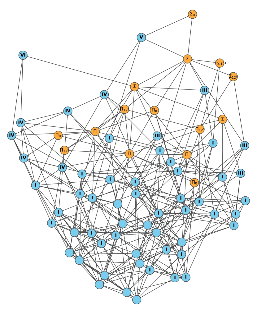
Figure 4. The superspecial Richelot isogeny graph for $p=47$. Vertices are labeled with their types; unlabeled vertices are Type-A, with trivial reduced automorphism group. Loops are omitted.

We may also compute the stationary distributions of the subgraphs $\Gamma^{SS}_{2}(2;47)^{J}$ and $\Gamma^{SS}_{2}(2;47)^{E}$. Recall from Table 1 that the degrees in these graphs are no longer regular: for example, a Type-A varieties have 15 isogenies to other Jacobians, while Type-I varieties have 14 isogenies to other Jacobians and a single isogeny to a product of elliptic curves. The stationary probability for a vertex $\mathcal{A}$ of type $T$ is

$$\tilde{\varphi}(\mathcal{A})=\frac{\deg\mathcal{A}}{g_{T}}\qquad\text{whenever $\mathcal{A}$ is of type $T$},$$

where $\deg\mathcal{A}$ is now the number of isogenies from $\mathcal{A}$ to vertices in the same graph, and $g_{T}$ is defined as above.

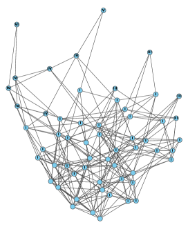
(a) Jacobian subgraph

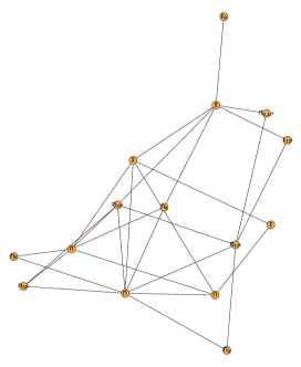
(b) Elliptic product subgraph

Figure 5. The subgraphs of $\Gamma^{SS}_{2}(2;47)$ supported on Jacobians (left) and elliptic products (right). Vertex positions are mantained with respect to Figure 4.

In this setting, the vertices which are not of Type-A in $\Gamma^{SS}_{2}(2;47)^{J}$ get more isolated, because they all have out-degree less than 15. On the other hand, the stationary distribution is uniformized slightly in $\Gamma^{SS}_{2}(47;p)^{E}$, because the vertices with larger automorphism groups have one, two or three fewer isogenies to Jacobians. This can be seen in Figure 5.

These phenomena generalize immediately to $\Gamma^{SS}_{2}(\ell;p)$ for all primes $\ell\neq p$, due to the generality achieved in Theorem 4.9.

Appendix A Experimental diameters and $\lambda_{\star}$ for $\Gamma^{SS}_{2}(2;p)$

The following table consists of experimental data computed for the graphs $G=\Gamma^{SS}_{2}(2;p)$, $J=\Gamma^{SS}_{2}(2;p)^{J}$ and $E=\Gamma^{SS}_{2}(2;p)^{E}$. The computed values are the diameters $d(G)$, $d(J)$ and $d(E)$, and the (scaled) second-largest eigenvalues of each graph. In particular, the second eigenvalues of $\Gamma^{SS}_{2}(2;p)$ support Conjecture 4.10. We use the notation $\tilde{\lambda}_{\star}=15\lambda_{\star}$.

$p$	$d(G)$	$d(J)$	$d(E)$	$\tilde{\lambda}_{\star}(G)$	$\tilde{\lambda}_{\star}(J)$	$\tilde{\lambda}_{\star}(E)$
17	3	3	2	10.671	9.203	3.000
19	3	3	2	11.072	10.016	1.833
23	3	4	2	10.241	8.993	4.102
29	4	4	4	10.472	9.522	6.460
31	3	4	2	11.183	10.516	5.748
37	4	4	2	10.797	10.025	5.372
41	5	5	6	11.436	10.098	7.837
43	4	4	2	11.153	10.650	5.495
47	4	5	4	11.131	10.526	7.580
53	5	5	4	11.060	10.769	6.145
59	5	5	5	11.475	10.447	7.927
61	5	6	3	11.451	11.037	6.978
67	5	4	4	11.563	11.210	7.537
71	5	5	4	11.341	10.885	7.183
73	5	5	4	11.577	11.129	7.575
79	5	5	3	11.216	10.774	6.576
83	6	6	5	11.262	11.023	8.241
89	6	6	6	11.307	10.681	8.418
97	5	5	6	11.494	11.089	7.973
101	6	6	7	11.192	10.817	8.474
103	6	6	5	11.217	10.980	8.644
107	6	6	6	11.379	11.203	7.344
109	6	6	4	11.168	10.985	6.549
113	6	6	6	11.386	11.156	7.593
127	6	6	4	11.612	11.383	7.522
131	7	6	8	11.525	11.373	8.179
137	6	6	6	11.648	11.440	7.193
139	6	6	5	11.528	11.424	7.682
149	7	7	8	11.534	11.407	8.131
151	6	6	4	11.387	11.285	7.338
157	6	7	6	11.508	11.291	8.489
163	6	6	6	11.638	11.376	8.012
167	7	7	6	11.494	11.359	8.116
173	7	7	7	11.631	11.408	8.077
179	7	7	8	11.586	11.459	8.075
181	6	7	6	11.347	11.267	8.270
191	7	7	7	11.461	11.348	8.307
193	6	6	5	11.537	11.431	7.754
197	7	7	8	11.295	11.207	7.789
199	7	7	6	11.361	11.261	8.041
211	7	7	6	11.610	11.522	7.933
223	7	7	7	11.484	11.339	8.334
227	7	7	7	11.480	11.397	8.110
229	7	7	6	11.605	11.486	8.076
233	7	7	6	11.523	11.420	7.672
239	8	7	8	11.581	11.431	8.246
241	7	7	6	11.507	11.342	8.233
251	8	7	8	11.568	11.371	8.585
257	8	7	8	11.636	11.462	8.315
263	7	7	7	11.539	11.433	7.640
269	8	7	8	11.448	11.337	8.405
271	7	7	6	11.537	11.482	8.037
277	7	8	6	11.530	11.396	7.935
281	7	7	8	11.479	11.366	8.297
283	7	7	7	11.582	11.504	8.272
293	8	8	8	11.582	11.430	8.390
307	7	7	7	11.614	11.535	8.244
311	8	8	7	11.507	11.383	8.411
313	8	7	7	11.645	11.480	8.439
317	8	8	7	11.543	11.495	7.922
331	7	7	7	11.505	11.450	8.018
337	7	7	7	11.613	11.542	8.005
347	8	8	8	11.520	11.457	8.185
349	8	8	8	11.465	11.407	8.485
353	8	8	8	11.561	11.490	8.143
359	8	8	8	11.556	11.500	8.311
367	8	8	7	11.553	11.463	8.352
373	8	8	7	11.475	11.411	8.259
379	8	7	7	11.474	11.408	8.202
383	8	8	7	11.548	11.492	8.351
389	8	8	9	11.582	11.544	8.280
397	8	8	7	11.593	11.523	8.368
401	8	8	8	11.558	11.492	8.315
409	8	8	8	11.626	11.575	8.354
419	9	8	10	11.555	11.472	8.552
421	8	8	6	11.614	11.569	8.015
431	8	8	8	11.585	11.512	8.276
433	8	8	9	11.615	11.532	8.516
439	8	8	8	11.509	11.459	8.389
443	8	8	9	11.501	11.458	8.287
449	8	8	8	11.546	11.499	8.178
457	8	8	8	11.539	11.460	8.429
461	9	8	9	11.588	11.513	8.452
463	8	8	9	11.514	11.458	8.394
467	8	8	8	11.608	11.561	8.332
479	8	8	9	11.579	11.524	8.202
487	8	8	8	11.546	11.512	8.320
491	8	8	8	11.606	11.529	8.217
499	8	8	8	11.492	11.457	8.168
503	9	8	8	11.606	11.529	8.209
509	9	9	9	11.607	11.542	8.431
521	10	8	10	11.618	11.566	8.295
523	8	8	8	11.596	11.545	8.338
541	8	8	8	11.518	11.469	8.255
547	8	8	8	11.591	11.555	8.282
557	9	8	10	11.528	11.490	8.277
563	9	9	8	11.542	11.486	8.360
569	9	8	10	11.573	11.525	8.366
571	8	8	8	11.605	11.560	8.262
577	8	8	8	11.612	11.490	8.438
587	9	9	9	11.628	11.565	8.362
593	9	8	10	11.642	11.565	8.446
599	9	9	9	11.535	11.481	8.449
601	8	8	8	11.553	11.518	8.219

Appendix B Explicit formulæ for genus-2 computations

This appendix collects useful formulæ for computing explicit Richelot isogenies, and identifying the reduced automorphism groups of abelian surfaces.

B.1. Richelot isogenies

Let $\mathcal{C}:y^{2}=F(x)$ be a genus-2 curve, with $F$ squarefree of degree $5$ or $6$. The Lagrangian subgroups of $\mathcal{J}({\mathcal{C}})[2]$ correspond to factorizations of $F$ into quadratics (of which one may be linear, if $\deg(F)=5$):

$$\mathcal{C}:y^{2}=F(x)=F_{1}(x)F_{2}(x)F_{3}(x)\,,$$

up to permutation of the $F_{i}$ and constant multiples. We call such factorizations quadratic splittings.

Fix one such quadratic splitting $\{F_{1},F_{2},F_{3}\}$; then the corresponding subgroup $K\subset\mathcal{J}({\mathcal{C}})[2]$ is the kernel of a $(2,2)$-isogeny $\phi:\mathcal{J}({\mathcal{C}})\to\mathcal{J}({\mathcal{C}})/K$. For each $1\leq i\leq 3$, we write $F_{i}(x)=F_{i,2}x^{2}+F_{i,1}x+F_{i,0}$. Now let

$$\delta=\delta(F_{1},F_{2},F_{3}):=\begin{vmatrix}F_{1,0}&F_{1,1}&F_{1,2}\\ F_{2,0}&F_{2,1}&F_{2,2}\\ F_{3,0}&F_{3,1}&F_{3,2}\end{vmatrix}\,.$$

If $\delta(F_{1},F_{2},F_{3})\not=0$, then $\mathcal{J}({\mathcal{C}})/K$ is isomorphic to a Jacobian $\mathcal{J}({\mathcal{C}^{\prime}})$, which we can compute using Richelot’s algorithm (see [5] and [39, §8]). First, let

$$G_{1}(x) :=\delta^{-1}\cdot(F_{2}^{\prime}(x)F_{3}(x)-F_{3}^{\prime}(x)F_{2}(x))\,,$$

$$G_{2}(x) :=\delta^{-1}\cdot(F_{3}^{\prime}(x)F_{1}(x)-F_{1}^{\prime}(x)F_{3}(x))\,,$$

$$G_{3}(x) :=\delta^{-1}\cdot(F_{1}^{\prime}(x)F_{2}(x)-F_{2}^{\prime}(x)F_{1}(x))\,.$$

Now the isogenous Jacobian is $\mathcal{J}({\mathcal{C}^{\prime}})$, where $\mathcal{C}^{\prime}$ is the curve

$$\mathcal{C}^{\prime}:y^{2}=G(x)=G_{1}(x)G_{2}(x)G_{3}(x)$$

and the quadratic splitting $\{G_{1},G_{2},G_{3}\}$ corresponds to the kernel of the dual isogeny $\phi^{\dagger}:\mathcal{J}({\mathcal{C}^{\prime}})\to\mathcal{J}({\mathcal{C}})$. The $F_{i}$ and $G_{i}$ are related by the identity

$$F_{1}(x_{1})G_{1}(x_{2})+F_{2}(x_{1})G_{2}(x_{2})+F_{3}(x_{1})G_{3}(x_{2})+(x_{1}-x_{2})^{2}=0\,.$$

Bruin and Doerksen present a convenient form for a divisorial correspondence $\mathcal{R}\subset\mathcal{C}\times\mathcal{C}^{\prime}$ inducing the isogeny $\phi$ (see [7, §4]):

(B.1) $$\mathcal{R}:\begin{cases}F_{1}(x_{1})G_{1}(x_{2})+F_{2}(x_{1})G_{2}(x_{2})=0\,,\\ F_{1}(x_{1})G_{1}(x_{2})(x_{1}-x_{2})=y_{1}y_{2}\,,\\ F_{2}(x_{1})G_{2}(x_{2})(x_{1}-x_{2})=-y_{1}y_{2}\,.\end{cases}$$

If $\delta(F_{1},F_{2},F_{3})=0$, then $\mathcal{J}({\mathcal{C}})/K$ is isomorphic to an elliptic product $\mathcal{E}\times\mathcal{E}^{\prime}$. Let $D(\lambda)$ be the discriminant of the quadratic polynomial $F_{1}+\lambda F_{2}$, and let $\lambda_{1}$ and $\lambda_{2}$ be the roots of $D(\lambda)$; then $F_{1}+\lambda_{1}F_{2}=U^{2}$ and $F_{1}+\lambda_{2}F_{2}=V^{2}$ for some linear polynomials $U$ and $V$. Now $F_{1}=\alpha_{1}U^{2}+\beta_{1}V^{2}$ and $F_{2}=\alpha_{2}U^{2}+\beta_{2}V^{2}$ for some $\alpha_{1}$, $\beta_{1}$, $\alpha_{2}$, and $\beta_{2}$, and since in this case $F_{3}$ is a linear combination of $F_{1}$ and $F_{2}$, we must have $F_{3}=\alpha_{3}U^{2}+\beta_{3}V^{2}$ for some $\alpha_{3}$ and $\beta_{3}$. Now, rewriting the defining equation of $\mathcal{C}$ as

$$\mathcal{C}:Y^{2}=\prod_{i=1}^{3}(\alpha_{i}U^{2}+\beta_{i}V^{2})\,,$$

it is clear that the elliptic curves

$$\mathcal{E}:Y^{2}=\prod_{i=1}^{3}(\alpha_{i}X+\beta_{i}Z)\quad\text{and}\quad\mathcal{E}^{\prime}:Y^{2}=\prod_{i=1}^{3}(\beta_{i}X+\alpha_{i}Z)$$

are the images of double covers $\pi:\mathcal{C}\to\mathcal{E}$ and $\pi^{\prime}:\mathcal{C}\to\mathcal{E}^{\prime}$ defined by $\pi((X:Y:Z))=(U:Y:V)$ and $\pi^{\prime}((X:Y:Z))=(V:Y:U)$, respectively. The product of these covers induces the isogeny $\phi:\mathcal{J}({\mathcal{C}})\to\mathcal{E}\times\mathcal{E}^{\prime}$.

B.2. Isogenies from elliptic products

Consider a generic pair of elliptic curves over $\Bbbk$, defined by

$$\mathcal{E}:y^{2}=(x-s_{1})(x-s_{2})(x-s_{3})$$

and

$$\mathcal{E}^{\prime}:y^{2}=(x-s_{1}^{\prime})(x-s_{2}^{\prime})(x-s_{3}^{\prime})\,.$$

We have $\mathcal{E}[2]=\{0_{\mathcal{E}},P_{1},P_{2},P_{3}\}$ and $\mathcal{E}^{\prime}[2]=\{0_{\mathcal{E}^{\prime}},P_{1}^{\prime},P_{2}^{\prime},P_{3}^{\prime}\}$ where $P_{i}:=(s_{i},0)$ and $P_{i}^{\prime}:=(s_{i}^{\prime},0)$. For each $1\leq i\leq 3$, we let

$$\psi_{i}:\mathcal{E}\longrightarrow\mathcal{E}_{i}:=\mathcal{E}/\langle{P_{i}}\rangle\quad\text{and}\quad\psi_{i}^{\prime}:\mathcal{E}^{\prime}\to\mathcal{E}_{i}^{\prime}:=\mathcal{E}^{\prime}/\langle{P_{i}^{\prime}}\rangle$$

be the quotient $2$-isogenies. These can be computed using Vélu’s formulæ [44].

The fifteen Lagrangian subgroups of $(\mathcal{E}\times\mathcal{E}^{\prime})[2]$ fall naturally into two kinds. Nine of the kernels correspond to products of $2$-isogeny kernels in $\mathcal{E}[2]$. Namely, for each $1\leq i,j\leq 3$ we have a subgroup

$$K_{i,j}:=\langle{(P_{i},0_{\mathcal{E}^{\prime}}),(0_{\mathcal{E}},P_{i}^{\prime})}\rangle\subset(\mathcal{E}\times\mathcal{E}^{\prime})[2]\,,$$

and a quotient isogeny

$$\phi_{i,j}:\mathcal{E}\times\mathcal{E}^{\prime}\to(\mathcal{E}\times\mathcal{E}^{\prime})/K_{i,j}\cong\mathcal{E}_{i}\times\mathcal{E}_{j}^{\prime}\,.$$

Of course, $\phi_{i,j}=\psi_{i}\times\psi_{j}$; we can thus compute $\phi_{i,j}$, and the codomains $\mathcal{E}_{i}\times\mathcal{E}_{j}^{\prime}$, using Vélu’s formulæ as above.

The other six kernels correspond to $2$-Weil anti-isometries $\mathcal{E}[2]\cong\mathcal{E}^{\prime}[2]$: they are

$$K_{\pi}:=\{(0_{\mathcal{E}},0_{\mathcal{E}^{\prime}}),(P_{1},P_{\pi(1)}^{\prime}),(P_{2},P_{\pi(2)}^{\prime}),(P_{3},P_{\pi(3)}^{\prime})\}\quad\text{for }\pi\in\operatorname{Sym}(\{1,2,3\})\,,$$

with quotient isogenies

$$\phi_{\pi}:\mathcal{E}\times\mathcal{E}^{\prime}\to\mathcal{A}_{\pi}:=(\mathcal{E}\times\mathcal{E}^{\prime})/K_{\pi}\,.$$

If the anti-isometry $P_{i}\mapsto P_{\pi(i)}^{\prime}$ is induced by an isomorphism $\mathcal{E}\to\mathcal{E}^{\prime}$, then $\mathcal{A}_{\pi}$ is isomorphic to $\mathcal{E}\times\mathcal{E}^{\prime}$; otherwise, it is the Jacobian of a genus-2 curve $\mathcal{C}_{\pi}$, which we can compute using the formulæ below (taken from [22, Proposition 4]).

Writing $\alpha_{i}:=x(P_{i})$ and $\beta_{i}:=x(P_{\pi(i)}^{\prime})$ for $1\leq i\leq 3$, let

$$a_{1} :=\frac{(\alpha_{3}-\alpha_{2})^{2}}{\beta_{3}-\beta_{2}}+\frac{(\alpha_{2}-\alpha_{1})^{2}}{\beta_{2}-\beta_{1}}+\frac{(\alpha_{1}-\alpha_{3})^{2}}{\beta_{1}-\beta_{3}}\,,$$

$$b_{1} :=\frac{(\beta_{3}-\beta_{2})^{2}}{\alpha_{3}-\alpha_{2}}+\frac{(\beta_{2}-\beta_{1})^{2}}{\alpha_{2}-\alpha_{1}}+\frac{(\beta_{1}-\beta_{3})^{2}}{\alpha_{1}-\alpha_{3}}\,,$$

$$a_{2} :=\alpha_{1}(\beta_{3}-\beta_{2})+\alpha_{2}(\beta_{1}-\beta_{3})+\alpha_{3}(\beta_{2}-\beta_{1})\,,$$

$$b_{2} :=\beta_{1}(\alpha_{3}-\alpha_{2})+\beta_{2}(\alpha_{1}-\alpha_{3})+\beta_{3}(\alpha_{2}-\alpha_{1})\,,$$

$$A :=\Delta^{\prime}\cdot a_{1}/a_{2}\text{ where }\Delta^{\prime}:=(\beta_{2}-\beta_{3})^{2}(\beta_{1}-\beta_{3})^{2}(\beta_{1}-\beta_{2})^{2}\,,$$

$$B :=\Delta\cdot b_{1}/b_{2}\text{ where }\Delta:=(\alpha_{2}-\alpha_{3})^{2}(\alpha_{1}-\alpha_{3})^{2}(\alpha_{1}-\alpha_{2})^{2}\,,$$

and finally

$$F_{1} :=A(\alpha_{2}-\alpha_{1})(\alpha_{1}-\alpha_{3})X^{2}+B(\beta_{2}-\beta_{1})(\beta_{1}-\beta_{3})Z^{2}\,,$$

$$F_{2} :=A(\alpha_{3}-\alpha_{2})(\alpha_{2}-\alpha_{1})X^{2}+B(\beta_{3}-\beta_{2})(\beta_{2}-\beta_{1})Z^{2}\,,$$

$$F_{3} :=A(\alpha_{1}-\alpha_{3})(\alpha_{3}-\alpha_{2})X^{2}+B(\beta_{1}-\beta_{3})(\beta_{3}-\beta_{2})Z^{2}\,.$$

Now the curve $\mathcal{C}_{\pi}$ may be defined by

$$\mathcal{C}_{\pi}:Y^{2}=-F_{1}(X,Z)F_{2}(X,Z)F_{3}(X,Z)\,.$$

The dual isogeny $\phi_{\pi}^{\dagger}:\mathcal{J}({\mathcal{C}_{\pi}})\to\mathcal{E}\times\mathcal{E}^{\prime}$ corresponds to the quadratic splitting $\{F_{1},F_{2},F_{3}\}$.

B.3. Identifying reduced automorphism types of Jacobians

We can identify the isomorphism class of a Jacobian $\mathcal{J}({\mathcal{C}})$ using the Clebsch invariants $A$, $B$, $C$, $D$ of $\mathcal{C}$, which are homogeneous polynomials of degree 2, 4, 6, and 10 in the coefficients of the sextic defining $\mathcal{C}$. These invariants should be seen as coordinates on the weighted projective space $\mathbb{P}(2,4,6,10)$: that is,

$$(A:B:C:D)=(\lambda^{2}A:\lambda^{4}B:\lambda^{6}C:\lambda^{10}D)$$

for all nonzero $\lambda$ in $\Bbbk$. The Clebsch invariants can be computed using a series of transvectants involving the sextic (see [33, §1]), but it is more convenient to use (for example) ClebschInvariants in Magma [4] or clebsch_invariants from the sage.schemes.hyperelliptic_curves.invariants library of Sage [43]. If $\mathcal{C}/\overline{\mathbb{F}}_{p}$ is superspecial, then $(A:B:C:D)$ are in $\mathbb{F}_{p^{2}}$.

To determine $\mathrm{RA}(\mathcal{J}({\mathcal{C}}))$ for a given genus-2 $\mathcal{C}$, we use necessary and sufficient conditions on the Clebsch invariants derived by Bolza [3, §11], given here in Table 6. These criteria involve some derived invariants: following Mestre’s notation [33], let

$$A_{11} =2C+\frac{1}{3}AB\,, A_{12} =\frac{2}{3}(B^{2}+AC)\,, A_{23} =\frac{1}{2}B\cdot A_{12}+\frac{1}{3}C\cdot A_{11}\,,$$

$$A_{22} =D\,, A_{31} =D\,, A_{33} =\frac{1}{2}B\cdot A_{22}+\frac{1}{3}C\cdot A_{12}$$

(recall again that $\operatorname{char}\Bbbk$ is not $2$ or $3$). Finally, the $R$-invariant is defined by

$$R^{2}=\frac{1}{2}\left|\begin{matrix}A_{11}&A_{12}&A_{31}\\ A_{12}&A_{22}&A_{23}\\ A_{31}&A_{23}&A_{33}\\ \end{matrix}\right|\,.$$

Type	$\mathrm{RA}(\mathcal{J}({\mathcal{C}}))$	Conditions on Clebsch invariants
Type-A	$1$	$R\not=0$, $(A:B:C:D)\not=(0:0:0:1)$
Type-I	$C_{2}$	$R=0$ and $A_{11}A_{22}\not=A_{12}$
Type-II	$C_{5}$	$(A:B:C:D)=(0:0:0:1)$
Type-III	$C_{2}^{2}$	$BA_{11}-2AA_{12}=-6D$, $D\not=0$,
		$CA_{11}+2BA_{12}=AD$, $6C^{2}\not=B^{3}$
Type-IV	$S_{3}$	$6C^{2}=B^{3}$, $3D=2BA_{11}$,
		$2AB\not=15C$, $D\not=0$
Type-V	$D_{2\times 6}$	$6B=A^{2}$, $D=0$, $A_{11}=0$, $A\not=0$
Type-VI	$S_{4}$	$(A:B:C:D)=(1:0:0:0)$

Table 6. The classification of reduced automorphism groups of Jacobian surfaces, with necessary and sufficient conditions on the Clebsch invariants for each type.

References

- [1] Sinan Aksoy, Fan Chung Graham, and Xing Peng, Extreme values of the stationary distribution of random walks on directed graphs, Adv. Appl. Math. 81 (2016), 128–155.
- [2] Reza Azarderakhsh, Brian Koziel, Matt Campagna, Brian LaMacchia, Craig Costello, Patrick Longa, Luca De Feo, Michael Naehrig, Basil Hess, Joost Renes, Amir Jalali, Vladimir Soukharev, David Jao, and David Urbanik, Supersingular Isogeny Key Encapsulation, http://sike.org, 2017.
- [3] Oskar Bolza, On binary sextics with linear transformations into themselves, American Journal of Mathematics 10 (1887), no. 1, 47–70.
- [4] Wieb Bosma, John J. Cannon, Claus Fieker, and Allan Steel, Handboook of Magma functions, 2.25 ed., January 2020.
- [5] Jean-Benoît Bost and Jean-François Mestre, Moyenne arithmético-géométrique et périodes des courbes de genre 1 et 2, Gaz. Math. Soc. France 38 (1988), 36–64.
- [6] Bradley W. Brock, Superspecial curves of genera two and three, Ph.D. thesis, Princeton University, 1993.
- [7] Nils Bruin and Kevin Doerksen, The arithmetic of genus two curves with (4, 4)-split Jacobians, Canadian Journal of Mathematics 63 (2011), no. 5, 992–1024.
- [8] Reinier Bröker, Kristin Lauter, and Andrew V. Sutherland, Modular polynomials via isogeny volcanoes, Mathematics of Computation 81 (2012), no. 278, 93–122.
- [9] Wouter Castryck, Thomas Decru, and Benjamin Smith, Hash functions from superspecial genus-2 curves using Richelot isogenies, Journal of Mathematical Cryptology 14 (2020), no. 1, 268–292, Proceedings of NuTMiC 2019.
- [10] Wouter Castryck, Tanja Lange, Chloe Martindale, Lorenz Panny, and Joost Renes, CSIDH: an efficient post-quantum commutative group action, Advances in Cryptology - ASIACRYPT 2018 - 24th International Conference on the Theory and Application of Cryptology and Information Security, Brisbane, QLD, Australia, December 2-6, 2018, Proceedings, Part III (Thomas Peyrin and Steven D. Galbraith, eds.), Lecture Notes in Computer Science, vol. 11274, Springer, 2018, pp. 395–427.
- [11] Denis X. Charles, Eyal Z. Goren, and Kristin E. Lauter, Families of Ramanujan graphs and quaternion algebras, Groups and symmetries: from Neolithic Scots to John McKay 47 (2009), 53–63.
- [12] Denis X. Charles, Kristin E. Lauter, and Eyal Z. Goren, Cryptographic hash functions from expander graphs, Journal of Cryptology 22 (2009), no. 1, 93–113.
- [13] Craig Costello and Benjamin Smith, The supersingular isogeny problem in genus 2 and beyond, Post-Quantum Cryptography - 11th International Conference, PQCrypto 2020, Paris, France, April 15-17, 2020, Proceedings (Jintai Ding and Jean-Pierre Tillich, eds.), Lecture Notes in Computer Science, vol. 12100, Springer, 2020, pp. 151–168.
- [14] Luca De Feo, David Jao, and Jérôme Plût, Towards quantum-resistant cryptosystems from supersingular elliptic curve isogenies, J. Math. Cryptol. 8 (2014), no. 3, 209–247.
- [15] Enric Florit and Benjamin Smith, An atlas of the superspecial richelot isogeny graph, Preprint: https://hal.inria.fr/hal-03094296, 2020.
- [16] E. Victor Flynn and Yan Bo Ti, Genus two isogeny cryptography, Post-Quantum Cryptography - 10th International Conference, PQCrypto 2019, Chongqing, China, May 8-10, 2019 Revised Selected Papers (Jintai Ding and Rainer Steinwandt, eds.), Lecture Notes in Computer Science, vol. 11505, Springer, 2019, pp. 286–306.
- [17] Mireille Fouquet and François Morain, Isogeny volcanoes and the SEA algorithm, Algorithmic Number Theory (Berlin, Heidelberg) (Claus Fieker and David R. Kohel, eds.), Springer Berlin Heidelberg, 2002, pp. 276–291.
- [18] Steven D. Galbraith, Christophe Petit, and Javier Silva, Identification protocols and signature schemes based on supersingular isogeny problems, 2016.
- [19] The GAP Group, GAP – Groups, Algorithms, and Programming, Version 4.11.0, 2020.
- [20] Pierrick Gaudry and Éric Schost, On the invariants of the quotients of the Jacobian of a curve of genus 2, International Symposium on Applied Algebra, Algebraic Algorithms, and Error-Correcting Codes, Springer, 2001, pp. 373–386.
- [21] Shlomo Hoory, Nathan Linial, and Avi Widgerson, Expander graphs and their application, Bulletin (New Series) of the American Mathematical Society 43 (2006).
- [22] Everett W. Howe, Franck Leprévost, and Bjorn Poonen, Large torsion subgroups of split Jacobians of curves of genus two or three, Forum Mathematicum 12 (2000), no. 3, 315–364.
- [23] Tomoyoshi Ibukiyama, Toshiyuki Katsura, and Frans Oort, Supersingular curves of genus two and class numbers, Compositio Mathematica 57 (1986), no. 2, 127–152.
- [24] David Jao and Luca De Feo, Towards quantum-resistant cryptosystems from supersingular elliptic curve isogenies, Post-Quantum Cryptography - 4th International Workshop, PQCrypto 2011, Taipei, Taiwan, November 29 - December 2, 2011. Proceedings (Bo-Yin Yang, ed.), Lecture Notes in Computer Science, vol. 7071, Springer, 2011, pp. 19–34.
- [25] Bruce W. Jordan and Yevgeny Zaytman, Isogeny graphs of superspecial abelian varieties and generalized Brandt matrices, 2020.
- [26] Toshiyuki Katsura and Katsuyuki Takashima, Counting richelot isogenies between superspecial abelian surfaces, Proceedings of the Fourteenth Algorithmic Number Theory Symposium (Steven D. Galbraith, ed.), vol. 4, The Open Book Series, no. 1, Mathematical Sciences Publishers, 2020, pp. 283–300.
- [27] David R. Kohel, Endomorphism rings of elliptic curves over finite fields, Ph.D. thesis, University of California at Berkley, 1996.
- [28] David A. Levin, Yuval Peres, and Elizabeth L. Wilmer, Markov chains and mixing times, American Mathematical Society, 2006.
- [29] Ke-Zheng Li and Frans Oort, Moduli of supersingular abelian varieties, Lecture Notes in Mathematics, vol. 1680, Springer-Verlag, Berlin, 1998. MR 1611305
- [30] László Lovász, Random walks on graphs: A survey, combinatorics, Paul Erdős is eighty, Bolyai Soc. Math. Stud. 2 (1993).
- [31] Ricardo Menares, Equidistribution of hecke points on the supersingular module, Proceedings of the American Mathematical Society 140 (2012), no. 8, 2687–2691.
- [32] Jean-François Mestre, La méthode des graphes. Exemples et applications, Proceedings of the international conference on class numbers and fundamental units of algebraic number fields (Katata), 1986, pp. 217–242.
- [33] Jean-François Mestre, Construction de courbes de genre 2 à partir de leurs modules, Effective methods in algebraic geometry, Springer, 1991, pp. 313–334.
- [34] Frans Oort, A stratification of a moduli space of abelian varieties, Prog. Math. 195 (2001).
- [35] Arnold K. Pizer, Ramanujan graphs and hecke operators, Bull. Amer. Math. Soc. (N.S.) 23 (1990), no. 1, 127–137.
- [36] Friedrich Julius Richelot, Essai sur une méthode générale pour déterminer les valeurs des intégrales ultra-elliptiques, fondée sur des transformations remarquables de ces trnscendates, Comptes Rendus Mathématique. Académie des Sciences. Paris 2 (1836), 622–627.
- [37] by same author, De transformatione integralium abelianorum primi ordinis commentatio, Journal für die Reine und Angewandte Mathematik 16 (1837), 221–341.
- [38] Alexander Rostovtsev and Anton Stolbunov, Public-key cryptosystem based on isogenies, Cryptology ePrint Archive, Report 2006/145, April 2006.
- [39] Benjamin Smith, Explicit endomorphisms and correspondences, Ph.D. thesis, University of Sydney, 2005.
- [40] Anton Stolbunov, Constructing public-key cryptographic schemes based on class group action on a set of isogenous elliptic curves, Adv. Math. Commun. 4 (2010), no. 2.
- [41] Andrew V. Sutherland, Identifying supersingular elliptic curves, LMS Journal of Computation and Mathematics 15 (2012), 317–325.
- [42] Katsuyuki Takashima, Efficient algorithms for isogeny sequences and their cryptographic applications, Mathematical Modelling for Next-Generation Cryptography. Mathematics for Industry (Singapore) (T. Takagi et al., ed.), vol. 29, Springer, 2018, pp. 97–114.
- [43] The Sage Developers, Sagemath, the Sage Mathematics Software System (Version 9.1), 2020, https://www.sagemath.org.
- [44] Jacques Vélu, Isogénies entre courbes elliptiques, Comptes Rendus Hebdomadaires des Séances de l’Académie des Sciences, Série A 273 (1971), 238–241.
- [45] Paul M. Weichsel, The Kronecker product of graphs, Proceedings of the American Mathematical Society 13 (1962), no. 1, 47–52 (en).