New Insights into Time Series Analysis IV:
Panchromatic and Flux Independent Period Finding Methods

Abstract

New time-series analysis tools are needed in disciplines as diverse as astronomy, economics and meteorology. In particular, the increasing rate of data collection at multiple wavelengths requires new approaches able to handle these data. The panchromatic correlated indices $K^{(s)}_{(fi)}$ and $L^{(s)}_{(pfc)}$ are adapted to quantify the smoothness of a phased light-curve resulting in new period-finding methods applicable to single- and multi-band data. Simulations and observational data are used to test our approach. The results were used to establish an analytical equation for the amplitude of the noise in the periodogram for different false alarm probability values, to determine the dependency on the signal-to-noise ratio, and to calculate the yield-rate for the different methods. The proposed method has similar efficiency to that found for the String Length period method. The effectiveness of the panchromatic and flux independent period finding methods in single waveband as well as multiple-wavebands that share a fundamental frequency is also demonstrated in real and simulated data.

1 Introduction

If the brightness variations of a variable star are periodic, one can fold the sparsely sampled light-curve with that period and inspect the magnitude as a function of phase plot. This will be equivalent to all the measurements of the star brightness taken within one period. The shape of the phased light-curve and the period allow one to determine the physical nature of variability (pulsations, eclipses, stellar activity, etc.). If the light-curve is folded with a wrong period, the magnitude measurements will be all over the place rather than align into a smoothly varying function of the phase. Other methods figure out the best period fitting a specific model into the phased light curve, like a sine function. The most common methods used in astronomy are the following: the Deeming method (Deeming, 1975), phase dispersion minimization (PDM - Stellingwerf, 1978; Dupuy & Hoffman, 1985), string length minimization (SLM - Lafler & Kinman, 1965; Dworetsky, 1983; Stetson, 1996; Clarke, 2002), information entropy (Cincotta et al., 1995), the analysis of variance (ANOVA - Schwarzenberg-Czerny, 1996), and the Lomb-Scargle periodogram and its extension using error bars (LS and LSG - Lomb, 1976; Scargle, 1982; Zechmeister & Kürster, 2009). All of these methods require as input the minimum frequency ($f_{min}$), the maximum frequency ($f_{max}$), and the sampling frequency (or the number of frequencies tested - $N_{freq}$). The input parameters and their constraints to determine reliable variability detections were addressed by Ferreira Lopes et al. (2018), where a summary of recommendations on how to determine the sampling frequency and the characteristic period and amplitude of the detected variations is provided. From these constraints, a good period finding method should find all periodic features if the time series has enough measurements covering nearly all variability phases (Carmo et al., 2020).

Light curve shape, non-Gaussianity of noise, non-uniformities in the data spacing, and multiple periodicities modify the significance of the periodogram and to increase completeness and reliability, more than one period finding method is usually applied to the data (e.g. Angeloni et al., 2012; Ferreira Lopes et al., 2015a, c). The capability to identify the "true" period is increased by using several methods (see Sect. 4.3). However, this does not prevent the appearance of spurious results. Therefore, new insights into signal detection which provide more reliable results are welcome mainly when the methods provide dissimilar periods. Moreover, the challenge of big-data analysis would benefit a lot from a single and reliable detection and characterization method. The present paper is part of a series of studies performed in the project called New Insight into Time Series Analysis (NITSA), where all steps to mining photometric data on variable stars are being reviewed. The selection criteria were reviewed and improved (Ferreira Lopes & Cross, 2016, 2017), optimized parameters to search and analyse periodic signals were introduced (Ferreira Lopes et al., 2018), and now new frequency finding methods are proposed to increase our inventory of tools to create and optimize automatic procedures to analyse photometric surveys. The outcome of this project is crucial if we are to efficiently select the most complete and reliable sets of variable stars in surveys like the VISTA Variables in the Via Lactea (VVV - Minniti et al., 2010; Angeloni et al., 2014), Gaia (Perryman, 2005), the Transiting Exoplanet Survey Satellite (TESS - Ricker et al., 2015), the Panoramic Survey Telescope and Rapid Response System (Pan-STARRS - Chambers et al., 2016), a high-cadence All-sky Survey System (ATLAS - Tonry et al., 2018), Zwicky Transient Facility (ZTF - Bellm et al., 2019) as well as the next generation of surveys like PLAnetary Transits and Oscillation of stars (PLATO - Rauer et al., 2014) and Large Synoptic Survey Telescope (LSST - Ivezic et al., 2008).

Many efforts are being performed to generalize for multi-band data the period finding methods. Süveges et al. (2012) utilized the principal component analysis to optimally extract the best period using multi-band data. However, the multi-band observations must be taken simultaneously that impose an important limitation to the method. On the other hand, VanderPlas & Ivezić (2015) introduces a general extension of the Lomb-Scargle method while Mondrik et al. (2015) for the ANOVA from single band algorithm to multiple bands not necessarily taken simultaneously. Indeed, methods combining the results from two different classes of period-determination algorithms are also being reached (Saha & Vivas, 2017). The current paper adds one piece to this puzzle. Section 2.1 describes the new set of periodic signal detection methods as well as their limitations and constraints. Next, numerical simulations are used to test our approach in Sect. 3. From this, the efficiency rate and the fractional fluctuation of noise (FFN) are determined. Real data are also used to support our final results (see Sect. 4). Finally, our conclusions are presented in Sect. 5.

2 Panchromatic and flux independent frequency finding methods

The Welch-Stetson variability index Stetson (1996) was generalized and new ones were performed by Ferreira Lopes & Cross (2016). From where the panchromatic and flux independent variability indices were proposed. These indices are used to discriminate variable stars from noise. To summarise, the panchromatic index is related to the correlation amplitude (or correlation height) while the second one computes the correlation sign, i.e. if the correlation value is negative or positive without taking into account the amplitude. The flux independent index provides correlation information that is weakly dependent on the amplitude or the presence of outliers. These features enable us to reduce the misclassification rate and improve the selection criteria. Moreover, this parameter is designed to compute correlation values among two or more observations. The correlation order ($s$), gives the number of observations correlated together, i.e., $s=2$ means correlation computed between pairs of observations and $s=3$ means that correlations are computed on triplets. However, these observations must be close in time, i.e., those observations are taken in an a interval time smaller much less than the main variability period. Inaccurate or incorrect outputs will be obtained if this restriction is not enforced. Therefore, the data sets and sources with observations close in time were named as correlated-data otherwise non-correlated-data.

The efficiency rate to detect variable stars is maximised using the panchromatic and flux independent variability indices when the number of correlations is increased, i.e when there is a strong variability between bins, but only slight differences between the measurements in each correlation bin. These variability indices only use those measurements that are close in time (i.e., a time interval much smaller than the variability period) and hence this constraint substantially reduced the number of possible correlations for sparse data. If we consider a light-curve folded on its true variability period, with little noise, we could calculate these indices using standard correlated observations grouped in time, missing the observations where too few meet the criteria of having at least $s$ closer than $\Delta\,T$ in time. Alternatively, all measurements can be used to compute the indices if the observations are grouped by phase instead of time. It is the main idea to support the Panchromatic and flux independent frequency finding methods.

For the main variability period, the observations closed in phase should return strong correlation values. Since many variable stars show most variation as a function of phase, and little variation from period to period, recalculating the indices this way should return indices that are as strong as those grouped by time. On the other hand, if the light-curve is folded on an incorrect period and the calculated phase is no longer a useful correlation measure, so correlations will be weaker, much like adding more noise to the data. The statistics considered in this paper are unlikely to be useful for data with multiple periodicities or if noise keeps its autocorrelation for phased data. In the next section, we propose an approach to compute the panchromatic and flux independent indices in phase and hence provide a new period finding method.

Be aware that, the definition of expected noise performed by Ferreira Lopes et al. (2015a) needs to be corrected, as pointed by the referee of the current paper. The authors provided the correct theoretical definition of expected noise but the mathematical expression was incorrect. In the case of statistically independent events, the probability that a given event will occur is obtained by dividing the number of events of the given type by the total number of possible events, according to the authors. There will always be 2 desired permutations (either all positive or all negative) for any s value. However, the total number of events is $2^{s}$, not $s^{2}$ as defined by the authors. The correct definition for expected noise value is then given by,

$$P_{s}=\frac{2}{2^{s}}=2^{(1-s)}$$ (1)

The relative differences between the old and new definition for $s=2$ and $s=4$ are zero while for $s=3$ is $\sim 11\%$. However, for s values larger than 4 these differences increase considerably. The authors have only used the noise definitions to set the noise level for s values smaller than 4, so far. Therefore, this mistake has not provided any significant error in the results of the authors to date.

2.1 New frequency finding methods

In common to other frequency finding methods, in our approach the light curve data are folded with a number of trial frequencies (periods). The trial frequency that produces the smallest scatter in the phase diagram according to some criteria is taken as the estimate of the real period of variations. In our approach we combine data from multiple bands with special transformations and characterize the phase diagram scatter using variability indices calculated from correlations of the phases (rather than correlations in the observation times, as they were used in previous works). The even-statistic (for more details see Paper II- Ferreira Lopes & Cross, 2017) was used to calculate the mean, median and deviation values. It only requires that the data must have even number of measurements (and if there is an odd number, the median value is not used) while the equations to compute these parameters are equal to the previous ones. This statement will be more important when the data has only a few measurements. On the other hand, these parameters assume equal values to the previous ones when the data has even number of measurements and they are quite similar for large data samples (typically bigger than 100).

Consider a generic time series observed in multiple wavebands with observations not necessarily taken simultaneously in each band. This could also mean a time series of the same sources taken by different instruments in single or multi-wavelength observations. The sub-index $w$ is used to denote each waveband. Using this notation, all data are listed in a single table where the $i^{th}$ observation is $\mathrm{\left[t_{i,w},\,\delta_{i,w}\right]}$ where $\delta_{i,w}$ is given by

$$\delta_{i,w}=\sqrt{\frac{n_{w}}{n_{w}-1}}\cdot\left(\frac{y_{i,w}-\bar{y_{w}}}{\sigma_{i,w}}\right),$$ (2)

where $n_{w}$ is the number of measurements, $y_{i,w}$ are the flux measurements, $\overline{y_{i,w}}$ is the even-mean computed using those observations inside of a $3\sigma$ clipped absolute even-median deviation (for more details see Paper II- Ferreira Lopes & Cross, 2017), and $\sigma_{i,w}$ denotes the flux errors of waveband $w$. One should note that greater success in searching for signals in multi-band light curves is found when a penalty and an offset between the bands are used (for more detail see Long et al., 2014; VanderPlas & Ivezić, 2015; Mondrik et al., 2015). However, these modifications require a more complex model since more constraints need to be added. For our purpose, we suppose that all wavebands used are well populated in order to provide a good estimation of the mean value.

The vector given by $\mathrm{\left[t_{i,w},\,\delta_{i,w}\right]}$ values contains data measured in either a single or multi-wavebands. For instance, w assumes a single value if a single waveband is used. Therefore the w sub-index is only useful to discriminate different wavebands and to compute the $\delta_{i,w}$. To simplify, the $w$ subindex is suppressed in the following steps. Therefore, the notation regarding all observations ($N$), observed in single or multi-wavebands by a single or different telescopes, is given by $\mathrm{\left[(t_{1},\,\delta_{1}),(t_{2},\,\delta_{2}),\cdots,(t_{N},\,\delta_{N})\right]}$. From which, the panchromatic ($PL^{(s)}$) and flux independent ($PK^{(s)}$) period finding indices are proposed as following;

1. First, consider a frequency sampling $\mathrm{F=[f_{1},f_{2},\cdots,f_{N_{freq}}]}$.

2. Next, the phase values $\Phi^{{}^{\prime}}=[\phi^{{}^{\prime}}_{1},\phi^{{}^{\prime}}_{2},\cdots,\phi^{{}^{\prime}}_{N}]$ are computed by $\mathrm{\phi^{{}^{\prime}}_{i}=t_{i}\times f_{1}-\lfloor t_{i}\times f_{1}\rfloor}$, where $t_{i}$ is the time and the $\mathrm{\lfloor\rfloor}$ means the ceiling function of $\mathrm{t_{i}\times f_{1}}$.

3. The phase values are re-ordered in ascending sequence of phase where $\Phi=[\phi_{1},\phi_{2},\cdots,\phi_{N}]$ and $\phi_{i}\leq\phi_{j}$ for all $i<j$, and the $\delta_{i}$ are also re-ordered with their respective phases. Where for each phase value we have $\mathrm{\left[(\phi_{1},\,\delta_{1}),(\phi_{2},\,\delta_{2}),\cdots,(\phi_{N},\,\delta_{N})\right]}$.

4. Next, the following parameter $Q$ of order $s$ is computed as;

   $$Q^{(s)}_{i}=\Lambda^{(s)}_{i,\,\cdots\,,i+s-1}\sqrt[s]{\left|\delta_{i}\,\cdots\,\delta_{i+s-1}\right|}$$ (3)

   where the $\Lambda^{(s)}$ function is given by

   $$\Lambda^{(s)}_{i}=\left\{\begin{array}[]{ll}+1&\qquad\mbox{if \,\, $\delta_{i}>0,\,\,\cdots\,,\,\delta_{i+s-1}>0$ };\\ +1&\qquad\mbox{if \,\, $\delta_{i}<0,\,\,\cdots\,,\,\delta_{i+s-1}<0$ };\\ 0&\qquad\mbox{if \,\, $\delta_{i}=0,\,\,\cdots\,,\,\delta_{i+s-1}=0$ };\\ -1&\qquad\mbox{otherwise}.\end{array}\right.$$ (4)

   Since we are assuming that the variables are periodic, when the period is correct, $\phi\sim 0$ should be equivalent to $\phi\sim 1$, so the last phases can be correlated with the first phases, i.e. if $s=2$, $Q^{(s)}_{N}$ correlates $\delta_{N}$ with $\delta_{1}$, and if $s=3$, $Q^{(s)}_{N-1}$ correlates $\delta_{N-1}$ with $\delta_{N}$ and $\delta_{1}$, and $Q^{(s)}_{N}$ correlates $\delta_{N}$ with $\delta_{1}$ and $\delta_{2}$, and so on. This consideration ensures the non repetition of any term and keeps the number of $Q^{(s)}$ terms equal to the number of observations. The sub-index $s$ sets the number of observations that will be combined (for more details see Paper I - Ferreira Lopes & Cross, 2016).

5. Finally, the period indices, equivalent to the flux-independent and panchromatic indices are given by,

   $$PK^{(s)}=\frac{N^{(+)}}{N}$$ (5)

   and,

   $$PL^{(s)}=\frac{1}{N}\sum_{i=1}^{N}Q^{(s)}_{i},$$ (6)

   where $N^{(+)}$ means the total number of positive correlations (see Eq. 4). Indeed, the total number of negative correlations ($N^{(-)}$) is given by $N^{(-)}=N-N^{(+)}$.

6. The steps ii to v are repeated for all frequencies, $f_{1}$ to $f_{N_{freq}}$.

One should be aware that $\delta_{i,w}$ values are strongly dependent on the average and hence incorrect values can be found for Algol type variable stars and time-series which have outliers, for example. In order to more accurately measure the average value only those observations within three times the absolute even-median deviations of the even-median were used to do this. Additionally, $\Lambda^{(s)}$ is a bit different from that proposed for the flux independent variability indices. The current version assumes $\Lambda^{(s)}=0$ if $\delta_{i}=0\,\,\cdots\,\,\delta_{i+s-1}=0$. This would produce $PK^{(s)}$ and $PL^{(s)}$ equal zero in the trivial case of all observations being exactly equal, e.g. a noiseless non-variable example, i.e., $y_{i}=y_{j}$ for all $i$ values (see two last panels of Fig. 2).

Figure 1: The $PK_{\rm max}^{(s)}$ as function of number of measurements for a sinusoidal function (see Eq. 7) for $s=2$ (solid black line), $s=3$ (solid red line), $s=4$ (solid blue line) where $N^{-}_{(min)}=2$ was adopted.

2.2 The maximum $\rm PK^{(s)}$ considering different signals

The maximum value allowed for the $PK^{(s)}$ parameter considering the true variability frequency ($\mathrm{f_{true}}$) of a signal is limited by the number of measurements which lead to $\Lambda^{(s)}=-1$, i.e., the minimum number of times that one of the consecutive phase observations has a value on the opposite side of the even-mean ($N_{(c)}$). This restriction limits the maximum value achievable by $PK^{(s)}$ ($PK_{\rm(max)}^{(s)}$). $PK_{\rm(max)}^{(s)}$ also varies with the order, $s$, since the number of $\Lambda^{(s)}=-1$ corresponding to observations on opposite sides of the even-mean varies with $s$. Indeed, $N_{(c)}$ depends on the shape of the signal. For instance, $N_{(c)}=1$ for a line, $N_{(c)}=2$ for a sinusoidal signal, $N_{(c)}=4$ for a eclipsing binary light curve. Moreover, if a set of measurements is given by a line $y=ax+b$ ($a\neq 0$), the number of negative correlation measurements will be $N^{-}_{(min)}=1$ for $s=2$, $N^{-}_{(min)}=2$ for $s=3$, and $N^{-}_{(min)}=3$ for $s=4$. Therefore, $N^{-}_{(min)}$, and hence the maximum $PK^{(s)}$ value, varies with s. These considerations can be expressed as following $N^{-}_{(min)}=N_{(c)}\times\left(s-1\right)$. Lastly, the general relation for $PK_{\rm(max)}^{(s)}$ can be written as

$$PK_{\rm(max)}^{(s)}=1-\frac{N^{-}_{(min)}}{N}=1-\frac{N_{(c)}\times\left(s-1\right)}{N}.$$ (7)

Figure 2: Phase diagrams for pulsating stars (RR, Ceph, RRblz), eclipsing binaries (type EA and EB), rotational variable stars (Rot), and white noise from uniform and normal distributions. The data and model are shown as black dots and solid lines, respectively. The even-mean value considering those measurements within three times the absolute even-median deviation is shown as orange dashed lines. Moreover, the $PK^{(2)}$ and $PL^{(2)}$ values for the real and modelled data are displayed at the bottom of each diagram.

A similar analytic equation for $PL^{(s)}$ index is not possible since it depends on the amplitude. On the other hand, two features of $PK^{(s)}$ can be seen in Eq. 7. First, $PK_{\rm(max)}^{(s)}$ values computed for two time-series having the same $N^{-}_{(\rm min)}$ value but a different number of observations differ (see Fig. 1). Second, all frequencies close to $\mathrm{f_{\rm true}}$ produce $PK^{(s)}\simeq PK_{\rm(max)}^{(s)}$, since $N>>N^{-}_{(\rm min)}$. These frequencies include the sub-harmonic frequencies of $\mathrm{f_{true}}$. Indeed, $\mathrm{f_{true}}$ will always return the $PK_{\rm(max)}^{(s)}$ value for time-series models or signals without noise (see blue lines on Fig. 2). However, when noise is included, statistical fluctuations can lead to the wrong identification of $\mathrm{f_{\rm true}}$. This means that the $PK^{(s)}$ and consequently $PL^{(s)}$ parameters can return a main frequency that implies a smooth phase diagram but is different to $\mathrm{f_{\rm true}}$.

The values of $N_{(c)}$ and therefore $N^{-}_{(min)}$ depend on the arrangement of observations around the even-mean and are intrinsically related to the signal-to-noise as discussed above (see Fig. 2). For instance, the detached eclipsing binary (EA) signal looks like noise if only the measurements outside of the eclipse are observed, e.g. if the phase fraction of the eclipses is $\lesssim\frac{2}{N}$. This means that the detection of the correct period using the $PK^{(s)}$ and $PL^{(s)}$ parameters will be extremely dependent on the number of observations at the eclipses. On the other hand, the RR Lyr (RR) objects show a small dispersion around the even-mean even if the signal-to-noise ratio (SNR) is a bit low. To summarize, the $PK^{(s)}$ power will have a peak for all frequencies which produce smooth phase diagrams, with the largest spectrum peak corresponding to the smallest $N^{-}_{(min)}$. On the other hand, the $PK_{\rm max}^{(s)}$ results in discrete values and so is more degenerate for a small number of observations.

Figure 2 shows the phase diagrams for a Cepheid (Ceph), a RR Lyrae (RR), a RR Lyrae having the Blazhko effect (RRblz), eclipsing binaries (EA and EB), a rotational variable (Rot), and two white noise light curves generated by uniform and normal distributions (for more details see Sect. 3). One thousand equally spaced phased measurements where used to plot each model and to compute the $PK^{(s)}$ shown in each panel ($PK_{(Model)}$). For these examples, we normalize amplitude to allow us to separate out the effects of the morphology of the light curves on these indices. As already mentioned, $PK^{(s)}$ is not directly dependent on the amplitude of the signal, as opposed to $PL^{(s)}$, which is. As expected, the model crosses the even-mean twice ($N^{-}_{(min)}=2$) for the Ceph, RR, RRblz, and Rot models giving $PK_{\rm max}^{(2)}=0.998$. For the eclipsing binaries the model crosses the even-mean four times, implying a $PK_{\rm max}^{(2)}=0.996$. Actually, the EA and EB models have $PK_{\rm max}^{(2)}=0.994$ due to fluctuations of the model about the even-median. Uniform and normal distributions (i.e., time series mimicking noisy data) $PK_{\rm max}^{(2)}=\gamma+2^{1-s}$ where $\gamma$ is a positive number related with the maximum fluctuation of positive correlations. However, the $PK_{\rm max}^{(s)}=1$ only happens when $\delta_{i}=0\,\forall\,i$ values, i.e. noiseless non-variation.

The $PL^{(s)}$ values for the data are biased by the amplitude, i.e., signals having different amplitudes will provide distinct values. Consider the index values computed using the data: the EA and EB signals have the smallest $PL^{(2)}$ values among all model tested due to their morphology, since the majority of measurements are near to the even-mean and hence the peak power is reduced. The Ceph, RR, and RRblz signals usually have large amplitudes and hence large $PL^{(2)}$ values. The highest $PL^{(2)}$ values are found for RR and Ceph signatures since there are a larger fraction of measurements distant from the even-mean than for the other models. The $PL^{(2)}$ value for RR stars is about half that found for the Rot model. This is a property related to the morphology of the phase diagram. Finally, the smallest values are found for pure-noise signals (normal and uniform distributions).

An examination of Eq. 7 can be used to estimate the theoretical expected value for any signal type. However, in real data, where noise is included, the $PK_{\rm max}^{(s)}$ values are smaller (see Fig. 2) since the values decrease with the increase in the dispersion of individual measurements about the even-mean. Therefore, $Rot$ and $EA$ models have the largest reduction in $PK_{\rm max}^{(s)}$. In contrast, the smallest reduction of $PK_{\rm max}^{(s)}$ is found for Ceph and RR models since the dispersion about even-mean is small. A detailed analysis of the weight of signal-to-noise ratio on $PK^{(s)}$ for different signal types is performed in the Sect. 3.

2.3 The optimal $s$ value

The optimal $s$ value ($s_{(opt)}$) will be found when the difference between $PK^{(s)}$ computed on the phase diagram folded using $\mathrm{f_{\rm true}}$ ($PK_{\rm max}^{(s)}$) and those ones found at other frequencies $PK_{\rm f_{other}}^{(s)}$ is maximum. This difference can be written as,

$$PK_{\rm(\mathrm{f_{\rm true}})}^{(s)}-PK_{\rm(f_{other})}^{(s)}\simeq PK_{\rm max}^{(s)}-PK_{\rm noise}^{(s)}$$ (8)

where we consider that $PK_{\rm(f_{other})}^{(s)}\simeq PK_{\rm noise}^{(s)}$ and compare the expressions 7 and 8

$$\frac{N^{+}_{\rm f_{true}}}{N}\simeq 1-\frac{N_{(c)}\times\left(s_{(\rm opt)}-1\right)}{N}$$ (9)

and hence,

$$s_{(\rm opt)}\simeq 1+\frac{\left(N-N^{+}_{\rm f_{true}}\right)}{N_{(c)}},$$ (10)

where $N^{+}_{\rm f_{true}}$ is the number of positive correlations for $\mathrm{f=f_{\rm true}}$. Equation 10 provides the $s$ value where the maximum difference between the $PK_{\rm(\mathrm{f_{\rm true}})}^{(s)}$ and $PK_{\rm(f_{other})}^{(s)}$ is found.

For high-SNR light curves, i.e. $N-N^{+}_{\rm f_{\rm true}}\rightarrow N_{(\rm c)}$, $s_{(\rm opt)}=2$ since for this case $N^{+}_{\rm f_{\rm true}}\rightarrow N$. Indeed, the $N^{+}_{\rm f_{\rm true}}$ is directly proportional to the SNR while $N_{(c)}$ is the opposite, i.e. the increase of SNR increases $N^{+}_{\rm f_{true}}$ and decreases $N_{(c)}$. Therefore, for low-SNR $N^{+}_{\rm f_{\rm true}}\rightarrow N/2$ and hence $s_{(\rm opt)}\approx 1+N/2\times N_{(\rm c)}$. However, at the limit, $N_{(c)}$ also tends to $N/2$ and hence $s_{(\rm opt)}\approx 2$. To summarize, the choice of $s$ value depends on the signal type and SNR since $N_{(\rm c)}$ and $N^{+}_{\rm f_{\rm true}}$ vary with both parameters. For instance, a large value of $N_{(\rm c)}$ is expected for EA binary systems whatever its SNR and hence a small $s$ value is recommended to increase the range of signal type detected. The choice of $s$ value must take all of these properties into account.

3 Numerical tests and simulations

Artificial variable stars were simulated using a similar set of models as those produced in paper III (for more details see Ferreira Lopes et al., 2018). Seven simulated time series were created that mimic rotational variables ($Y_{(Rot)}$), detached eclipsing binaries ($Y_{(EA)}$), eclipsing binaries ($Y_{(EB)}$), pulsating stars ($Y_{(Ceph)}$, $Y_{(RR)}$, $Y_{(RRblz)}$), and white noise ($Y_{(Uniform)}$ and $Y_{(Normal)}$). The Ceph, RR, RRblz, EA, and Rot models were based on the CoRoT light curves CoRoT-211626074, CoRoT-101370131, CoRoT-100689962, CoRoT-102738809, and CoRoT-110843734, respectively. The variability types were previously identified by Debosscher et al. (2007); Poretti et al. (2015); Paparó et al. (2009); Chadid et al. (2010); Maciel et al. (2011); Carone et al. (2012) and De Medeiros et al. (2013) while the variability period and amplitudes were reviewed by Ferreira Lopes et al. (2018). The models of variable stars were found using harmonic fits having $12$, $12$, $12$, $24$, $24$, and $6$ coefficients for $Ceph$, $RR$, $RRblz$, $EA$, $EB$, and $Rot$ variable stars, respectively. The white noise simulations given by a normal distribution were used to determine the fractional fluctuation of noise (FFN). The Ceph, RR, RRblz, EA, and Rot models were used to realistically test and illustrate our approach.

The efficiency rate of any frequency finding method depends mainly on the signal type, the signal-to-noise ratio, and the number of observations. Therefore, three sets of simulations having $20$, $60$, and $100$ measurements for an interval of $\rm SNR$ (see Eq. 11) ranging from $\sim 1$ to $\sim 20$ were created for the models found in Fig. 2. In particular, $20\%$ of measurements were randomly selected at the eclipses for EA and EB simulations. This is required because these simulations look like noise if no measurement is found at the eclipses, and is justified because any light-curves that are processed with period-finding algorithms in NITSA must already have been selected as variables, so eclipsing binaries with few measurements must have a relatively high fraction at the eclipses. There will be a selection effect against binaries with narrow eclipses, since the probability of them being detected as variables is reduced. Values sorted randomly from a normal distribution were used to add noise to the simulations and the error-bars were set to be the differences between the model and simulated data. The error bars are not relevant to compute the $PK^{(s)}$ values. However, they are necessary to determine $PL^{(s)}$ parameters. The $\rm SNR$ was computed as,

$$SNR=\frac{A}{2.96\times eMAD(\delta_{y})}$$ (11)

where $A$ is the signal amplitude, $\delta_{y}$ are the residuals (observed minus its predicted measurement), and $eMAD$ is the even-median of the absolute deviations from the even-median. The $eMAD$ is a slight modification of median absolute deviation from median ($MAD$). The $2.96\times eMAD(\delta_{y})$ is equivalent to two times the standard deviation but it is a robust estimate of the standard deviation when outliers are considered (e.g. Hoaglin et al., 1983). For completeness, other estimates of the SNR where the model is not required were tested (e.g. Rimoldini, 2013). According to our tests, the latter usually overestimates the SNR compared with those values computed by Eq. 11.

Figure 3: $PK^{(s)}$ as a function of the number of measurements for orders 2, 3, and 4. The results for significance levels of $99\%$ (orange), $95\%$ (grey), and $90\%$ (blue) are in different colors. The dashed lines indicate the $\rm FFN_{(s)}$ for models while the solid, red line shows the expected value for the noise (see Sect.3.1).

3.1 Fractional Fluctuation of Noise (FFN)

The fractional fluctuation of noise for signal detection is related to the level for which the figure of merit of the methods (e.g., power, in the classical periodogram) is not expected to exceed more than a fraction of times due to stochastic variation (or noise) on the input light curve. Indeed, the FFN mimics a false alarm probability since it sets the power value above which a certain percentage of spurious signals are found. Indeed, there are many difficulties of estimating FAPs in realistic astronomical time series (for more detail see Koen, 1990; Sulis et al., 2017; VanderPlas, 2018) and hence FFN only means the lower empirical limit to find a reliable signal. The expected value of the flux-independent index, $K_{\rm fi}^{(s)}$, for white noise is analytical defined as $P_{s}=2^{s-1}$ (see Sect. 2). The same equation can be applied to $PK^{(s)}$ since $K_{\rm fi}^{(s)}$ and $PK^{(s)}$ are based on the same concept. Therefore, the $FFN_{(s)}$ can be defined as,

$$FFN_{(s)}=P_{s}+\Delta=\sqrt{\frac{\alpha}{N}}+\beta$$ (12)

where $\alpha$ and $\beta$ are real positive numbers. $\beta$ must be larger than $P_{s}$ since it is a threshold for white noise. $10^{7}$ Monte Carlo simulations using a normal distribution were run with the number of measurements ranging from $10$ to $1000$ in order to compute the free parameters for Eq. 12. Figure 3 shows the mean values of $PK^{(s)}$ above which $1\%$ (orange dots), $5\%$ (grey dots), and $10\%$ (blue dots) of simulated data are found. The $FFN_{(s)}$ models are shown as dashed lines and the free parameters of the models are presented in Table 1. The minimum values of $FFN_{(s)}$ are found when $N\rightarrow\infty$. For this condition the $FFN_{(s)}$ estimates have values above the noise (see Table 1). The scatter found for small numbers of measurements (typically less than $20$) is related to the discrete values allowed for $PK^{(s)}$ (for more details see Ferreira Lopes & Cross, 2016). The results shown in Fig. 3 are quite similar for all uncorrelated zero-mean noise distributions.

Table 1: The constraints to $\rm FFN_{s}$ models (see Eq. 12) which delimit $99\%$, $95\%$, and $90\%$ of white noise, respectively.

	$99\%$		$95\%$		$90\%$
order	$\alpha$	$\beta$	$\alpha$	$\beta$	$\alpha$	$\beta$
$\rm FFN_{(2)}$	$0.9459$	$0.5107$	$0.5350$	$0.5177$	$0.4377$	$0.5112$
$\rm FFN_{(3)}$	$1.2321$	$0.2541$	$0.6150$	$0.2696$	$0.4784$	$0.2625$
$\rm FFN_{(4)}$	$1.0937$	$0.1316$	$0.4511$	$0.1482$	$0.2380$	$0.1482$

The $FFN_{(s)}$ can be used as a reference to remove unreliable signals that lead to random phase variations in any survey, whatever the wavelength observed. This property is related to the weak dependence of $PK^{(s)}$ on amplitude, error bars, or outliers according to Ferreira Lopes & Cross (2017). Indeed, spurious periods that lead to smooth phase diagrams will break this constraint. On the other hand, the period that produces the main peak in the periodogram can be related with a phase diagram which has gaps for common methods like PDM and LSG. This happens because the function used to measure the periodogram can interpret this arrangement of measurements as a smooth phase diagram. This result can lead to the highest periodogram peak when the signal is not well defined and/or when a small number of epochs are available. On the other hand, the periods that lead to folded phase diagrams with gaps may not have many correlated measurements and hence they will not leads to peaks in the $PK^{(s)}$ and $PL^{(s)}$ periodogram. Indeed, the main peak of the periodogram will be the arrangement of measurements that leads to the largest correlation value.

Figure 4: $PK^{(s)}$ as a function of signal-to-noise ratio for order 2 ($s=2$) for the variable stars models shown in the Fig. 2. Each column displays the results for $20$ (left column of panels), $60$ (middle panels), and $100$ (right-hand columns of panels) measurements while each row presents the results for different variable types: Cepheid, RRlyrae, RRblz, EA, EB, and Rot models. Box plots containing $90\%$ of the data are shown. The even-median values for each box are marked by a solid red line while the dashed blue lines show the expected value for the noise.

3.2 Dependency on the signal-to-noise ratio

The $Ceph$, $RR$, $RRblz$, $EA$, $EB$, and $Rot$ models (for more details see Sect. 3) were used to analyze the $PK^{(s)}$ values for the main variability signal. $PK^{(s)}$ values were computed using $10^{7}$ Monte Carlo simulations for SNR ranging from $1$ to $20$. The simulations were created for $s=2$, $s=3$, and $s=4$. The results for $s=3$ and $s=4$ show lower efficiency than those found for $s=2$ for lower SNR values, as expected from Sect. 2.3. The results for larger orders, $s$, provide better results than those found for $s=2$, for high signal-to-noise time-series, having large number of measurements (see Sect. 2.3). Therefore, we only show the results for $s=2$. Figure 4 shows the $PK^{(s)}$ as function of SNR for $s=2$. The results are displayed using box plots instead of error bars because $PK^{(s)}$ results in discrete values and its distribution is not symmetric. A box plot range that includes $90\%$ of results was used, and the red line sets the middle of the distribution. The main results can be summarized as follows:

• The maximum value achieved by $PK^{(s)}$ is limited by the number of measurements for all SNR. Moreover, this effect is also observed for higher s orders in agreement with the values estimated by Eq. 7 (see Fig. 1).

• $PK^{(s)}$ tends to $PK_{(max)}^{(s)}$ for simulations using $20$, $60$, and $100$ measurements and high SNR for Ceph, RR, RRblz, EB, and Rot models. The same trend having a slower growth is also observed for EA. Indeed, $PK^{(s)}$ values are improved for EA models when the number of measurements, mainly at the eclipses, is increased. About $\sim 50\%$ of $PK^{(s)}$ values for SNR $=3$ are found below the expected noise value when the time-series has 20 measurements. This number is reduced to less than $\sim 10\%$ when more than 60 measurements are available.

• The dispersion of $PK^{(s)}$ values decreases with the number of measurements for all values of SNR. The effect is less noticeable for EA models. This happens because the simulated time series looks like noise when most of the measurements are sorted outside of eclipses.

• About $\sim 95\%$ of $PK^{(2)}$ values are above $P_{2}$ values for the whole range of SNR for Ceph, RR, RRblz, EB, and Rot simulations using $60$ and $100$ measurements. This is also true for the simulations containing 20 measurements for $\rm SNR>2$. On the other hand, the EA model shows $PK^{(2)}$ values around the noise level for the whole range of SNR on the simulations containing $20$ measurements. The reason for this behaviour is the same as explained in the last item.

• The time-series like EA and EB models have the lowest $PK^{(s)}$ values among all models analysed.

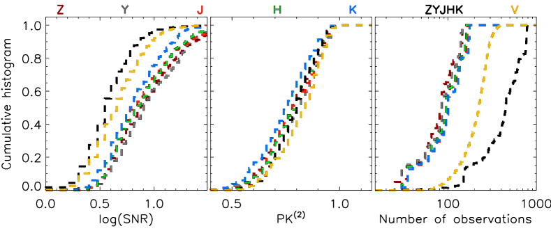
Figure 5: Cumulative histograms of SNR, $PK^{2}$, and number of measurements for WVSC1 and CVSC1 stars. The results are shown for Z (brown), Y (grey), J (red), H (green), K (blue), V (yellow) as well as the panchromatic (black) data.

In summary, the probability of finding $\rm PK^{(s)}$ values above the noise is dependent on the number of measurements, SNR, and signal type, as expected. For all simulations, when the number of measurements is increased, we can measure reliable periods at lower SNR. The simulations for higher $s$ order are quite similar to those found for $s=2$.

4 Testing the method on real data

A robust numerical simulation is complex because it usually does not reproduce the correlated nature of the noise intrinsic to the data as well as variations related to the instrumentation. Many constraints are required to provide realistic simulations such as a wide range of amplitudes, error bars, outliers, and correlated noise, to name a few. However, the simulation of the $PK^{(s)}$ power is facilitated because: (a) the amplitude can be a free parameter since $PK^{(s)}$ is only weakly dependent on it; (b) the even mean values (see Eq. 2) are computed using those observations within three times the absolute even-median deviation, which effectively reduces the outliers weight on zero point estimation ($\overline{y_{w}}$, see Eqn. 2) but all epochs are considered to compute the powers; (c) the correlated nature of successive measurements is reduced since they are computed using phase diagrams. On the other hand, a robust simulation for $PL^{(s)}$ covering all important aspects of it is difficult because $PL^{(s)}$ has a strong dependence on amplitude, outliers, and error bars. Therefore, the discussions in the previous sections only address the constraints on $PK^{(s)}$.

The $PK^{(s)}$ and $PL^{(s)}$ methods can be tested on real data using existing variable stars catalogues. The WFCAMCAL variable stars catalogue (WVSC1) having $280$ stars (Ferreira Lopes et al., 2015a) and the Catalina Survey Periodic Variable star catalogue (CVSC1) having $\sim 47000$ sources (Drake et al., 2014) were used to estimate the efficiency rate of our new period finding methods. The WVSC1 was created from the analysis of the WFCAM Calibration 08B release (WFCAMCAL08B - Hodgkin et al., 2009; Cross et al., 2009). More information about the design, the data reduction, the layout, and about variability analysis of this database are described in detail in Hambly et al. 2008; Cross et al. 2009; Ferreira Lopes et al. 2015a. The WFCAMCAL database is a useful dataset to test single and panchromatic wavelength period finding methods. To summarize, WFCAM database contains panchromatic data ($ZYJHK$ wavebands) that were observed to calibrate the UKIDSS surveys Lawrence et al. 2007. A sequence of filters $JHK$ or $ZYJHK$ were observed within a few minutes during each visit the fields. These sequences were repeated in a semi-regular way that leads to an uneven sampling having large seasonal gaps. On the other hand, the CVSC1 has a huge amount of objects, with seventeen variable stars types that were visually inspected by the authors.

In order to perform a straightforward comparison between the results, the SNR of WVSC1 and CVSC1 stars were also estimated using Eq. 11. Also, the number of measurements and the $PK^{(2)}$ values were computed. Figure 5 shows the cumulative histograms of SNR and number of measurements for WVSC1 and CVSC1 stars. The results for each waveband as well as for panchromatic data are shown by different colours. About $\sim 90\%$ of WVSC1 single waveband has $SNR>\sim 3$ while this number decreases to $\sim 70\%$ for the CVSC1 and panchromatic data. The WVSC1 single waveband data have a number of measurements ranging from $\sim 30$ to $\sim 150$ while CVSC1 stars have a number from $\sim 100$ to $\sim 300$. When the panchromatic data is considered, the number of measurements increases considerably by a factor $\sim 5$ compared with WVSC1 single waveband. However, the SNR are smaller than those found for single wavebands. In general, the SNR for panchromatic wavebands are smaller than those found for CVSC1 stars.

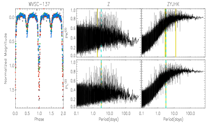
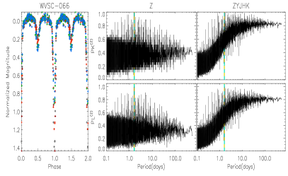
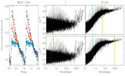
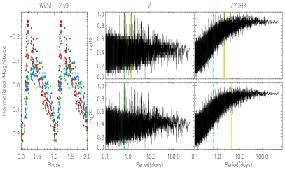
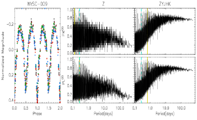
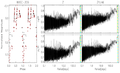
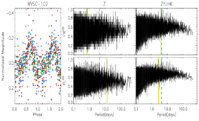
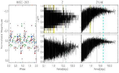
Figure 6: Phase diagrams of panchromatic data (left panels) and the $PK^{(s)}$ and $PL^{(s)}$ normalized periodogram for Z and ZYJHK wavebands (right panels). The cross symbols in the phase diagrams set the measurement of Z (brown), Y (grey), J (green), H (red), and K (blue) wavebands. The dashed green lines indicate the published variability periods while the full yellow lines indicate the periods related with the largest peak in the periodogram.

Understanding the peculiarities of the sample tested is crucial when analysing the efficiency rate of our approach. Therefore we summarize how the period searches were performed to find periods for WVSC1 and CVSC1 stars. Ferreira Lopes et al. (2015a) selected about $6651$ targets to which four period finding methods were applied. Next, the ten best ranked periods in each of the four methods were selected. For each period a light curve model was created using harmonics fits. Finally, the very best period was chosen as that with the smallest $\chi^{2}$ with respect to all ranked periods; On the other hand, the period search for $\sim 154$ thousand CVSC1 sources was made using the Lomb Scargle method. Next, the main periods were analysed using the Adaptive Fourier Decomposition (AFD) method (Torrealba et al., 2015) in order to determine the main variability period and reduce the number of sources to be visually inspected ($112$ thousand). Additionally, the periods of a large number of the sources were improved and corrected by the authors. Many of the variability periods of WVSC1 and CVSC1 were related to sub-harmonics of their true period and the final results were set after visual inspection.

The following sections discuss the WVSC1 and CVSC1 variable stars from the viewpoint of $PK^{(s)}$ and $PL^{(s)}$ parameters. The periodogram, the efficiency rate, and the peculiarities of our approach are analysed. For that, we perform the period search using the SLM, LSG, and PDM methods besides the panchromatic and flux independent methods. A frequency range of $(2/T_{max})d^{-1}$ to $30d^{-1}$ was explored and we evenly sampled this frequency range with a frequency step of $\frac{1}{300\times T_{max}}$, where $T_{max}$ is the total time span. The frequency sampling constrains a maximum phase shift of $0.1$ that allows us to detect the large majority of signal types (for more detail see Paper III). A quick visual inspection was performed on some of WVSC1 and CVSC1 to test our analysis in the next sections. The main goal of this work is to propose a new period finding method instead of checking the reliability of the periods in the WVSC1 and CVSC1 catalogues.

4.1 Periodogram and efficiency rate

The $PK^{(2)}$ and $PL^{(2)}$ periodogram were computed for the WVSC1 and CVSC1 stars. For better visualization, the differential panchromatic light curve (see Fig. 6) was obtained by subtracting the even-median from the magnitudes in each light curve. As a result, light curves with zero mean are produced. The $PK^{(s)}$ and $PL^{(s)}$ parameters do not use any kind of transformation to combine measurements at different wavelengths. However, a better way to combine multi-wavelength data is an open question.

Figure 6 shows the phase diagrams and their normalized periodogram for some WVSC1 stars. The phase diagrams (left panels) show the folded panchromatic data while the periodogram considering single and panchromatic wavebands are displayed in the centre and right panels respectively. The periodogram for a large part of CVSC1 stars are quite similar to those found for panchromatic data, i.e., periodogram for sources having more measurements and smaller SNR than for the WVSC1 single waveband. The main results can be summarized as follows:

• $PK^{(2)}$ has more than one peak related with the maximum power for WVSC-239 and WVSC-263, i.e., this means that $PK^{(s)}_{(max)}$ indicates more than one viable period. The number of such periods gives the ”degeneracy” of a particular arrangement of measurements in the phase diagram. This number increases as the number of measurements decreases (see Eq. 7).

• The main period found by $PK^{(2)}$ is not the same as that obtained by $PL^{(2)}$. This means that the maximum number of positive correlations is not the same as the maximum correlation power. Besides, the ”degeneracy” of periods found for $PK^{(2)}$ is not observed in the $PL^{(2)}$ periodogram.

• $PK^{(2)}$ and $PL^{(2)}$ periodogram for the Z waveband show a scatter around the expected noise level. Additionally, the WVSC-054 and WVSC-209 periodogram show an increase in $PK^{(2)}$ for long periods. Indeed, this behaviour is observed in all wavebands and hence it is an attribute of the proposed method.

• $PK^{(2)}$ for panchromatic data increases with periods up to a maximum of around $5$ days and then levels off and drops slightly for longer periods for almost all sources. These sources have variability periods of less than $5$ days. This behaviour is not found for WVSC-209 and WVSC-102. Indeed, WVSC-102 has a variability period of $589$ days and hence the trend observed is different to the others. On the other hand, WVSC-209 has a low-SNR signal. Therefore, this trend is related with the variability period and SNR. Indeed, the phase diagram keeps part of the correlation information when the light curve is folded using a test period bigger than the true variability period.

• $PK^{(2)}$ and $PL^{(2)}$ periodogram have peaks at the previous measured (true) variability periods of WVSC1 stars. However, the period related with the largest peak is not always the true variability period.

• The panchromatic data have lower SNR. Indeed, no clear signal can be observed in WVSC-263. This could mean that the signal shape is very different from one band to another, or a signal or seasonal variation is present in a single waveband, or the variability period is wrong, to name the most likely possibilities.

To summarize, the $PK^{(s)}$ and $PL^{(s)}$ periodogram indicate the arrangement of measurements in the phase diagram that maximize the correlation signal and power, respectively. Therefore, the $PK^{(s)}$ and $PL^{(s)}$ parameters can be used to identify the periods that lead to a smooth phase diagram from the viewpoint of correlation strength.

Table 2: Accuracy considering two approaches; the main period ($E_{(M)}$) and the main period plus its sub-harmonic and overtone. We consider that there is agreement if the relative difference is smaller than $1\%$.

	Z		Y		J		H		K		ZYJHK		V
	$E_{(M)}$	$E_{(MH)}$	$E_{(M)}$	$E_{(MH)}$	$E_{(M)}$	$E_{(MH)}$	$E_{(M)}$	$E_{(MH)}$	$E_{(M)}$	$E_{(MH)}$	$E_{(M)}$	$E_{(MH)}$	$E_{(M)}$	$E_{(MH)}$
$\rm PK^{(2)}$	$0.30$	$0.55$	$0.30$	$0.59$	$0.30$	$0.60$	$0.29$	$0.59$	$0.23$	$0.50$	$0.19$	$0.40$	$0.24$	$0.51$
$\rm PL^{(2)}$	$0.20$	$0.46$	$0.22$	$0.49$	$0.22$	$0.50$	$0.28$	$0.57$	$0.17$	$0.44$	$0.14$	$0.27$	$0.25$	$0.53$
LSG	$0.10$	$0.27$	$0.09$	$0.29$	$0.09$	$0.34$	$0.09$	$0.26$	$0.11$	$0.31$	$0.09$	$0.32$	$0.20$	$0.87$
PDM	$0.17$	$0.50$	$0.26$	$0.59$	$0.25$	$0.62$	$0.27$	$0.62$	$0.22$	$0.57$	$0.26$	$0.69$	$0.22$	$0.88$
SLM	$0.30$	$0.55$	$0.30$	$0.59$	$0.29$	$0.63$	$0.28$	$0.59$	$0.22$	$0.50$	$0.15$	$0.32$	$0.25$	$0.49$

4.2 Accuracy

The accuracy was measured considering the main signal(s) detected by the $PK^{(2)}$ and $PL^{(2)}$ methods. Indeed, the largest power of $PK^{(s)}$ periodogram can be related to more than one period. Therefore, all periods related to the largest periodogram peak were considered to measure the accuracy, i.e., the recovery fraction of variability periods. Two parameters to measure the accuracy were considered: $E_{(M)}$ - when the main period is detected; $E_{(MH)}$ - when the main variability period ($P_{Lit}$), measured in Ferreira Lopes et al. (2015a), or its sub-harmonic, or overtone is found. Indeed, the processing time of each method was not taken into account in this discussion. A new approach to reduce the running time necessary to perform period searches will be addressed in a forthcoming paper in this series. Those signals found within $\pm 1\%$ of the variability period were considered as detected. Table 2 shows the results for individual wavebands as well as for the panchromatic data. The main results can be summarized as:

• The accuracy is lower than $100\%$ for all methods and data tested. However, new estimates of Catalina variability periods have been produced recently (e.g. Papageorgiou et al., 2018) and the CVSC1 combines the results found by PDM, LSG, and STR methods for all wavebands to determine the best variability period. Therefore, the accuracy for both datasets is larger than that displayed in Table 2 if these results are taken into consideration.

• $PK^{(2)}$ has the highest efficiency rate considering only the main period ($E_{(M)}$) for the Z, Y, J, H, and K wavebands. The efficiency rate of $PK^{(2)}$ for the V waveband and panchromatic data is similar to that found for the SLM and $PL^{(2)}$ methods. $E_{(M)}$ decreases form Z to K wavebands because the first ones have larger SNR.

• The $E_{(MH)}$ values for Z, Y, J, H, and K for $PK^{(2)}$ and SLM are quite similar and they have the highest accuracy for the Z and Y wavebands. On the other hand, PDM has the highest $E_{(MH)}$ values for H, ZYJHK, and V wavebands. Indeed, the $E_{(MH)}$ values for PDM and LSG are quite similar for the V waveband.

• The $E_{(M)}$ for $PL^{(2)}$ is always smaller than that found for $PK^{(2)}$ except for V band where it is $4\%$ lower for $PK^{(2)}$.

• The highest $E_{(M)}$ is found for $PK^{(2)}$ method while the highest $E_{(MH)}$ is found for the PDM method. The accuracy found for LSG method is quite similar to that found for PDM method for V waveband while in other wavebands the PDM method has twice the accuracy. Indeed, this difference is reduced by a few percent if a higher relative error is considered. Indeed, the $P_{Lit}$ found by the ZYJHK wavebands are refined using the SLM method (for more details see Ferreira Lopes et al., 2015a). On the other hand, the V waveband results were computed using Lomb-Scargle and refined using reduced $\chi^{2}$ (for more details see Drake et al., 2014). Therefore, the accuracy can be biased by the approach used to improve the variability period estimation. Indeed, a deep discussion about how to determine accurately the variability period and its error is found in the third paper of this series (for more details see Ferreira Lopes et al., 2018).

• The panchromatic data do not significantly increase the efficiency rate for any method. The panchromatic data provides a larger number of measurements but a smaller SNR compared with those found for single wavebands (see Fig. 5).

• The efficiency rate of $PK^{(2)}$, $PL^{(2)}$, and SLM is strongly decreased for V and panchromatic data. This is related with the smaller SNR of these data. It indicates a strong dependence of the $PK^{(2)}$ and $PL^{(2)}$ methods on the SNR.

The periods detected by PDM are also detected by the LSG method. Moreover, almost all periods detected using the PK, PL, and STR methods are also found by the LSG method. The periods detected using LSG or PDM which are not found by other methods belong mainly to a few types: W UMa ($\sim 61\%$), EA ($\sim 13\%$), RR Lyr on first overtone ($\sim 10\%$), and RR Lyr on several modes ($\sim 2\%$), measured using the ratio of the number of missed sources to the total number of sources missed. Indeed, the largest miss-rate is found for the multi-periodic RR Lyr-type when the relative number of sources are considered, i.e. the fraction of missed sources divided by the number of sources detected for each variability type. As expected, the multi-periodic periods have the largest miss-rate since the current approach is not designed to select these periods. From quick visual inspection on phased data of the periods found by methods other than PDM and LSG the following concerns have been raised: the period found is a higher harmonic or overtone of that found in the literature; the phase diagram is not always smooth; the period found sometimes produces a smooth phase diagram but the period found is different or has a relative difference larger than $1\%$. This means that STR, PK, and PL methods are more likely to return spurious periods or higher harmonics of the main variability period since the majority of the sources missed belong to these groups.

On the other hand, about $\sim 8\%$ of the Catalina periods do not correspond to our periods. We also made a quick visual inspection of the phased data using the periods found by Catalina and those found by us. As a result, we verify that the large majority (more that $\sim 70\%$) of phase diagrams of this subsample produce smoother phase diagrams using our periods than those found using Catalina periods (see third row of panels of Fig. 7). Indeed, this assumes that the true or main variability period should be that one which produces the smoothest phase diagram.

In summary, the $PK^{(s)}$ and $PL^{(s)}$ methods can be used as a new tool to find periodic signals. In fact, they are more efficient than all methods tested if high SNR data are considered. As a rule, the new approach can be used in the same fashion as other period finding methods. One should be aware that, the lower efficiency rate for small SNR, probable bias for longer periods, and the multiple-periods given by $PK^{(s)}$must be taken into account.

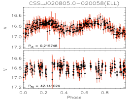
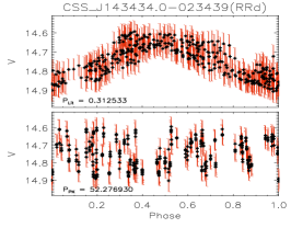
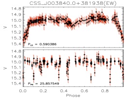
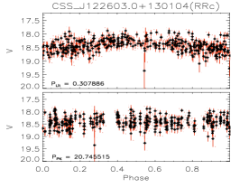
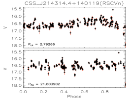
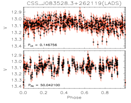
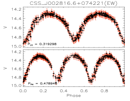
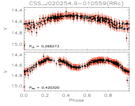
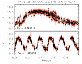
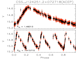
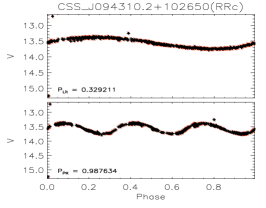
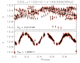
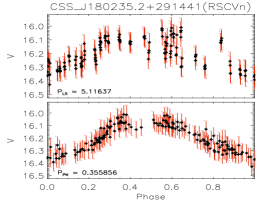
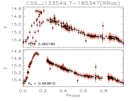
Figure 7: Phase diagrams for CVSC1 stars considering the published variability period ($P_{Lit}$) and that one found by $PK^{(2)}$ method ($P_{PK}$). The star name is shown on the top of each diagram while the periods are in the bottom left corners.

4.3 Cautionary notes on period searching

The main variability period is assumed to be that one which provides the smoothest phase diagram. Indeed, the periodicity of many signals in oversampled data like CoRoT and Kepler light curves (e.g. Paz-Chinchón et al., 2015; Ferreira Lopes et al., 2015b) can be easily identified by looking directly at the light curve. This may not include low SNR multi-periodic signals. On the other hand, the signals in undersampled data can only can be identified by eye using phase diagrams. In both cases, the phase diagram should be smooth at the main variability period. However, more than one period can lead to smooth phase diagrams. In fact, due to the nature of the analysis of big-datasets it is highly likely that some observational biases exist or that pathological cases arise where the combination of random or correlated errors, nearby sources, mimic expected variations. Therefore, additional information must be put together to solve this puzzle. For instance, photometric colours, amplitudes, nearby saturated sources, crowded sky regions, distances, and other information are crucial to confirm the period reliably.

All configurations that produce smooth phase diagrams return the peaks in the $PK^{(s)}$ method. The current approach was designed to find the main variability period from the viewpoint of correlation. Indeed, the harmonic periods also provide peaks in the periodogram since the number of consecutive measurements that cross the even-mean is only a small increase (see Eq. 7), often smaller than random crosses due to noise. Actually, other signals not related to the main variability period also can lead to smooth phase diagrams and hence they also have peaks close to $PK^{(s)}_{(max)}$. Moreover, incorrect periods also can be obtained if all configurations that lead to smoother phase diagrams are not addressed.

The $PK^{(s)}$ method is a useful tool to find all periods that lead to smooth phase diagrams. Other methods, e.g. the string length, or PDM method, or the fitting of truncated Fourier series also lead to smooth phase diagrams. For completeness, the most prominent peaks should be examined to evaluate the best candidate for the main variability signal. The best period can be assumed to be the one that leads to the smallest $\chi^{2}$ of a model computed from the phase diagram (e.g. Drake et al., 2014; Ferreira Lopes et al., 2015a; Torrealba et al., 2015). Figure 7 shows five cases from CVSC1 where topics discussed here are a hindrance. In each row of panels are presented some examples as follows:

• First row of panels: stars where the $PK^{(2)}$ method does not identify the correct variability period. In these cases, an examination of the phase diagrams for the other peaks in $PK^{(2)}$ may help to find the correct value.

• Second row of panels: stars for which a smooth phase diagram is not clearly defined by either CVSCI or the $PK^{(2)}$ method. Therefore, both the $P_{Lit}$ and $P_{PK}$ estimate may be wrong. Indeed, Drake et al. 2014 use other criteria to define the period reliably. However, this analysis is hindered if other information besides of light curve are not available.

• Third row of panels: both the $P_{Lit}$ and $P_{PK}$ estimates produce smooth phase diagrams. However, they are not sub-harmonics of one another. This means that both periods are sub-harmonic of the main variability period or one of them is incorrect. Indeed, these systems also might be a complex systems with multiple periodicities, e.g. an eclipsing binary where one of component is a pulsating star. These examples illustrate that the criterion of having a smooth phase diagram per se is not enough to define the variability period.

• Fourth row of panels: the variability period found by $PK^{(2)}$ method is an overtone (greater than 2) of the variability period. Therefore, it indicates that the efficiency rate discussed in Sect. 4.2 is better if higher sub-harmonics are considered.

• Last row of panels: stars where $P_{Lit}$ is wrong or inaccurate. $P_{PK}$ returns smoother phase diagrams than those using $P_{Lit}$. Indeed, the $PK^{(s)}$ period for CSS_J110010.1+165359 appears to be a sub-harmonic of the true variability period. The wrong period determination can result in a misclassification since many of parameters used for classification are derived from the variability period.

The WVSC1 stars have similar features to those discussed using CVSC1 stars. A quick visual inspection was performed to support our remarks. A few stars look like those found on the last row of panels shown in Fig. 7 in both samples. Indeed, the main goal of this work is to provide a new way to find and analyse variability time-series.

5 Conclusions

Two new ways to search variability periods are proposed. These methods are not derived from any previous period finding method. The $PK^{(s)}$ method is characterized by presenting ordinates in the range $0$ to $1$, does not have a strong dependence on the amplitude of the signal, and also has an analytical equation to determine the $\rm FFN$. Moreover, the weight of outliers is reduced since the method only considers the signs of the correlation signal. These are unique features that allow us to determine a universal false alarm probability, i.e., the cut-off values that can be applied to any time-series, where it mainly depends on the SNR of the light curve. In contrast, the $PL^{(s)}$ method uses the correlation values and provides complementary information about the variability period.

The $PK^{(s)}$ and $PL^{(s)}$ methods were compared with the LSG, PDM, and SLM methods from real and simulated data having single and multi-wavelength data. As result, the efficiency rate found for LSG and PDM methods are better than all other methods for sub-samples having low ($<3$) or high ($>3$) SNR data. On the other hand, $PK^{(s)}$ and $PL^{(s)}$ efficiency is similar to that found for SLM method for data in both constraints. As expected, the accuracy of all methods is increased for data having high SNR.

In fact, the statistics considered in this paper are unlikely to be useful for data with multiple periodicities. The current methods were recent applied in the entire data of VVV survey (Ferreira Lopes et al., 2020) from where the periods estimated from five period finding method can be found. This paper is the second of this series about period search methods. Our next paper will provide our summary of recommendation to reduce running time and improve the periodicity search on big-data sets.

6 Data and Materials

The data underlying this article are available in the Catalina repository and in the WFCAM Science Archive - WSA. A friendly version of the data also can be shared on reasonable request to the corresponding author.

References

- Angeloni et al. (2012) Angeloni R., Di Mille F., Ferreira Lopes C. E., Masetti N., 2012, ApJ, 756, L21
- Angeloni et al. (2014) Angeloni R., et al., 2014, A&A, 567, A100
- Bellm et al. (2019) Bellm E. C., et al., 2019, PASP, 131, 018002
- Carmo et al. (2020) Carmo A., Ferreira Lopes C. E., Papageorgiou A., Jablonski F. J., Rodrigues C. V., Drake A. J., Cross N. J. G., Catelan M., 2020, Boletin de la Asociacion Argentina de Astronomia La Plata Argentina, 61C, 88
- Carone et al. (2012) Carone L., et al., 2012, A&A, 538, A112
- Chadid et al. (2010) Chadid M., et al., 2010, A&A, 510, A39
- Chambers et al. (2016) Chambers K. C., et al., 2016, arXiv e-prints,
- Cincotta et al. (1995) Cincotta P. M., Mendez M., Nunez J. A., 1995, ApJ, 449, 231
- Clarke (2002) Clarke D., 2002, A&A, 386, 763
- Cross et al. (2009) Cross N. J. G., Collins R. S., Hambly N. C., Blake R. P., Read M. A., Sutorius E. T. W., Mann R. G., Williams P. M., 2009, MNRAS, 399, 1730
- De Medeiros et al. (2013) De Medeiros J. R., et al., 2013, A&A, 555, A63
- Debosscher et al. (2007) Debosscher J., Sarro L. M., Aerts C., Cuypers J., Vandenbussche B., Garrido R., Solano E., 2007, A&A, 475, 1159
- Deeming (1975) Deeming T. J., 1975, Ap&SS, 36, 137
- Drake et al. (2014) Drake A. J., et al., 2014, ApJS, 213, 9
- Dupuy & Hoffman (1985) Dupuy D. L., Hoffman G. A., 1985, International Amateur-Professional Photoelectric Photometry Communications, 20, 1
- Dworetsky (1983) Dworetsky M. M., 1983, MNRAS, 203, 917
- Ferreira Lopes & Cross (2016) Ferreira Lopes C. E., Cross N. J. G., 2016, A&A, 586, A36
- Ferreira Lopes & Cross (2017) Ferreira Lopes C. E., Cross N. J. G., 2017, A&A, 604, A121
- Ferreira Lopes et al. (2015a) Ferreira Lopes C. E., Dékány I., Catelan M., Cross N. J. G., Angeloni R., Leão I. C., De Medeiros J. R., 2015a, A&A, 573, A100
- Ferreira Lopes et al. (2015b) Ferreira Lopes C. E., et al., 2015b, A&A, 583, A122
- Ferreira Lopes et al. (2015c) Ferreira Lopes C. E., Leão I. C., de Freitas D. B., Canto Martins B. L., Catelan M., De Medeiros J. R., 2015c, A&A, 583, A134
- Ferreira Lopes et al. (2018) Ferreira Lopes C. E., Cross N. J. G., Jablonski F., 2018, MNRAS, 481, 3083
- Ferreira Lopes et al. (2020) Ferreira Lopes C. E., et al., 2020, MNRAS, 496, 1730
- Hambly et al. (2008) Hambly N. C., et al., 2008, MNRAS, 384, 637
- Hoaglin et al. (1983) Hoaglin D. C., Mosteller F., Tukey J. W., 1983, Understanding robust and exploratory data anlysis. New York: John Wiley
- Hodgkin et al. (2009) Hodgkin S. T., Irwin M. J., Hewett P. C., Warren S. J., 2009, MNRAS, 394, 675
- Ivezic et al. (2008) Ivezic Z., et al., 2008, Serbian Astronomical Journal, 176, 1
- Koen (1990) Koen C., 1990, ApJ, 348, 700
- Lafler & Kinman (1965) Lafler J., Kinman T. D., 1965, ApJS, 11, 216
- Lawrence et al. (2007) Lawrence A., et al., 2007, MNRAS, 379, 1599
- Lomb (1976) Lomb N. R., 1976, Ap&SS, 39, 447
- Long et al. (2014) Long J. P., Chi E. C., Baraniuk R. G., 2014, arXiv e-prints, p. arXiv:1412.6520
- Maciel et al. (2011) Maciel S. C., Osorio Y. F. M., De Medeiros J. R., 2011, New Astron., 16, 68
- Minniti et al. (2010) Minniti D., et al., 2010, New Astron., 15, 433
- Mondrik et al. (2015) Mondrik N., Long J. P., Marshall J. L., 2015, ApJ, 811, L34
- Papageorgiou et al. (2018) Papageorgiou A., Catelan M., Christopoulou P.-E., Drake A. J., Djorgovski S. G., 2018, ApJS, 238, 4
- Paparó et al. (2009) Paparó M., Szabó R., Benkő J. M., Chadid M., Poretti E., Kolenberg K., Guggenberger E., Chapellier E., 2009, in Guzik J. A., Bradley P. A., eds, American Institute of Physics Conference Series Vol. 1170, American Institute of Physics Conference Series. pp 240–244, doi:10.1063/1.3246453
- Paz-Chinchón et al. (2015) Paz-Chinchón F., et al., 2015, preprint, (arXiv:1502.05051)
- Perryman (2005) Perryman M. A. C., 2005, in Seidelmann P. K., Monet A. K. B., eds, Astronomical Society of the Pacific Conference Series Vol. 338, Astrometry in the Age of the Next Generation of Large Telescopes. p. 3
- Poretti et al. (2015) Poretti E., Le Borgne J. F., Rainer M., Baglin A., Benkő J. M., Debosscher J., Weiss W. W., 2015, Monthly Notices of the Royal Astronomical Society, 454, 849
- Rauer et al. (2014) Rauer H., et al., 2014, Experimental Astronomy, 38, 249
- Ricker et al. (2015) Ricker G. R., et al., 2015, Journal of Astronomical Telescopes, Instruments, and Systems, 1, 014003
- Rimoldini (2013) Rimoldini L., 2013, preprint, (arXiv:1304.6715)
- Saha & Vivas (2017) Saha A., Vivas A. K., 2017, AJ, 154, 231
- Scargle (1982) Scargle J. D., 1982, ApJ, 263, 835
- Schwarzenberg-Czerny (1996) Schwarzenberg-Czerny A., 1996, ApJ, 460, L107
- Stellingwerf (1978) Stellingwerf R. F., 1978, ApJ, 224, 953
- Stetson (1996) Stetson P. B., 1996, PASP, 108, 851
- Sulis et al. (2017) Sulis S., Mary D., Bigot L., 2017, IEEE Transactions on Signal Processing, 65, 2136
- Süveges et al. (2012) Süveges M., et al., 2012, MNRAS, 424, 2528
- Tonry et al. (2018) Tonry J. L., et al., 2018, PASP, 130, 064505
- Torrealba et al. (2015) Torrealba G., et al., 2015, MNRAS, 446, 2251
- VanderPlas (2018) VanderPlas J. T., 2018, ApJS, 236, 16
- VanderPlas & Ivezić (2015) VanderPlas J. T., Ivezić Ž., 2015, ApJ, 812, 18
- Zechmeister & Kürster (2009) Zechmeister M., Kürster M., 2009, A&A, 496, 577