Efficient Index-based Approaches for Personalized $k$-wing Search

Abstract

Computing a $k$-wing structure in a bipartite graph has found extensive real applications such as spam group detection, word and document clustering, etc. The existing approaches take quadratic time to compute a $k$-wing and need to explore the entire bipartite graph. Given the fact that real bipartite graphs can be substantially large and dynamically updated, and the queries of $k$-wing are issued quite frequently in real applications, the existing approaches would be too expensive. In this paper, we propose an optimal algorithm for personalized $k$-wing search based on novel indices, i.e., the algorithm runs in linear time with respect to the result size. We propose two indices for $k$-wing search: first, EquiWing, $k$-wing equivalence relationship is proposed and is used to summarize the input bipartite graph $G$; second, EquiWing-Comp, it is a more compact version of EquiWing, which is achieved by integrating our proposed k-butterfly loose approach and discovered hierarchy properties. Moreover, we propose an upper bound for the change in wing number which can be $\geq 1$ and also provide an efficient localized update of the EquiWing and EquiWing-Comp with an edge insertion/deletion in $G$. We perform extensive experimental studies in real-world, large-scale graphs to validate the efficiency and effectiveness of EquiWing-Comp, which has achieved at least an order of magnitude speedup in cohesive subgraph search over EquiWing.

I Introduction

Bipartite cohesive subgraph. Bipartite graphs are an interesting structure that can be used to represent large heterogeneous data. Many real-world networks can be modeled using bipartite graphs such as social networks, online shopping sites, and author-paper networks (Fig. 1). For a given bipartite graph $G=(U,V,E)$, a bipartite cohesive subgraph $B=(U^{\prime},V^{\prime},E^{\prime})$ is the subgraph of $G$ such that $U^{\prime}$ and $V^{\prime}$ are extensively connected via edges in $E^{\prime}$. A bipartite cohesive subgraph $B=(U^{\prime},V^{\prime},E^{\prime})$ is unaffected by the connections within $U^{\prime}$ or $V^{\prime}$ themselves.

Applications. Finding bipartite cohesive subgraphs has a rich literature with examples such as word and document clustering [Dhillon:2001:CDW:502512.502550], spam group detection in the web [Gibson:2005:DLD:1083592.1083676], and sponsored advertisement [fain2006sponsored]. The objective of finding all the bipartite cohesive subgraphs i.e. bipartite cohesive subgraph detection is to aim the entire bipartite graph and generally apply a global criterion to provide macroscopic information.

Existing models. Due to a large number of applications for bipartite cohesive subgraphs in the real-world, bipartite graphs have been studied using various structures such as bicliques [abidipivot], $(\alpha,\beta)$-core [liu2020efficient], and $k$-wing [zou2016bitruss, DBLP:conf/wsdm/SariyuceP18]. These three structures correspond to cliques, $k$-core, and $k$-truss in the general graphs. However, we selected $k$-wing as the founding structure of our bipartite cohesive subgraphs as: (1) $k$-wing provides better cohesive and stable relationships than the naive metrics of the number of vertices/edges in the bipartite graphs [DBLP:conf/wsdm/SariyuceP18]. (2) $k$-wing follows the hierarchical modeling, wherein by changing the $k$ value, we can obtain a collection of $k$-wings which details different levels of cohesiveness (cohesiveness of a subgraph is $\propto$ $k$) for the given query vertex [DBLP:conf/wsdm/SariyuceP18]. (3) finding all the $k$-wings in a bipartite graph $B$ requires a polynomial runtime [DBLP:conf/wsdm/SariyuceP18], while the denser subgraph models based on maximal biclique require exponential time [kumar1999trawling, rome2005towards]. We observe the superiority for $k$-wing over $(\alpha,\beta)$-core and biclique by considering the example (Fig. 1) of two authors working in the same area can be in each other’s bipartite cohesive subgraph without knowing each other.

Figure 1: In an author-paper network, author $v_{0}$ and $v_{3}$ may not have worked together but have the same area of interest.

Personalized bipartite cohesive subgraph. Distinct vertices in a bipartite graph may have distinct properties, which requires the microscopic analysis, i.e. personalized. There are many real-world applications where people are more interested in personalized bipartite cohesive subgraphs rather than all possible bipartite cohesive subgraphs. For example, analysis in co-authorship networks (e.g. DBLP) for improving the collaboration among the authors for potential future collaborations and project fundings [arnab2016analysis, Sozio2010cocktail]. This specific problem of exploring personalized bipartite cohesive subgraphs can be used for a wide variety of applications such as personalized recommendation for products [zhang2019domain] and hotels [kaya2019hotel], identifying potential websites for banner advertisements [hunter2013structural], efficient training of the employees on the internal projects by choosing the optimal team for an employee [zhang2017enterprise] and speculating the drug-target interactions [yamanishi2013chemogenomic].

In this paper, we study personalized bipartite cohesive subgraph search based on $k$-wing. Given a bipartite graph $G(U,V,E)$, a query vertex $q\in U\cup V$ and a possible integer $k$, the personalized $k$-wing search returns all the maximal $k$-wings containing $q$. The selection of $k$-wing is based on its possession of the features of bicliques (high density) and $(\alpha,\beta)$-core (hierarchical properties and polynomial-time efficiency) simultaneously.

The problem of personalized bipartite subgraph can be addressed by adapting the algorithms proposed for finding all the bipartite cohesive subgraphs [DBLP:conf/wsdm/SariyuceP18]. Unfortunately, the existing method [DBLP:conf/wsdm/SariyuceP18] only addresses the $k$-wing decomposition, which computes wing number of each edge whereas algorithms for retrieving $k$-wing subgraphs strictly satisfying butterfly connectivity are not provided. Recently approaches like [DBLP:conf/icde/Wang0Q0020] have been proposed to improve the wing decomposition, however, butterfly connectivity problem remains unaddressed. Therefore, prioritize the problem of finding personalized bipartite subgraph rather than wing decomposition. We first attempt to solve a personalized $k$-wing search by using the computed wing number only, i.e., our baseline solution. However, due to the high time complexity of checking butterfly connectivity, the baseline solution runs in $O(|E|^{2})$ where $|E|$ is the number of edges in a bipartite graph. As such, the baseline cannot be applied to real applications with extensive number of personalized $k$-wing queries due to its high time complexity.

TABLE I: Notations and their descriptions

Notation	Description
$G=(U,V,E)$	A simple bipartite graph $G$.
EW$(\raisebox{1.5pt}{$\chi$},\Upsilon)$	The summarized index EquiWing.
EW-C$(\raisebox{1.5pt}{$\chi$},\Upsilon)$	The compressed index EquiWing-C.
$u,w,u_{i}$($v,x,v_{i}$)	vertices $\in U$ (vertices $\in V$).
$\nu,\mu,\nu_{i},\mu_{i}$	super nodes $\in\raisebox{1.5pt}{$\chi$}$.
$\psi(e)$	The wing number of an edge $e\in E$
$\mathbin{\rotatebox[origin={c}]{90.0}{$\hourglass$}}_{uvxy}$	The butterfly composed of $u,x\in U$ and $v,y\in V$.
$N(e)/\Gamma(u)$	The set of neighboring edges/vertices of $e/u$ of a graph.
$e_{1}\stackrel{{\scriptstyle\mathclap{\hugefont\mbox{$\mathbin{\rotatebox[origin={c}]{90.0}{$\hourglass$}}^{k}$}}}}{{=}}e_{2}$	$e_{1}$ and $e_{2}$ are $k$-wing equivalent.
$e_{1}\xLeftrightarrow{k}e_{2}$, $\mathbin{\rotatebox[origin={c}]{90.0}{$\hourglass$}}_{1}\xLeftrightarrow{k}\mathbin{\rotatebox[origin={c}]{90.0}{$\hourglass$}}_{2}$	$e_{1}$ and $e_{2}$ ($\mathbin{\rotatebox[origin={c}]{90.0}{$\hourglass$}}_{1}$ and $\mathbin{\rotatebox[origin={c}]{90.0}{$\hourglass$}}_{1}$) are k-butterfly connected.
$\nu_{1}\xLeftrightarrow{>k}\nu_{2}$, $\mathbin{\rotatebox[origin={c}]{90.0}{$\hourglass$}}_{1}\xLeftrightarrow{>k}\mathbin{\rotatebox[origin={c}]{90.0}{$\hourglass$}}_{2}$	$\nu_{1}$ and $\nu_{2}$ ($\mathbin{\rotatebox[origin={c}]{90.0}{$\hourglass$}}_{1}$ and $\mathbin{\rotatebox[origin={c}]{90.0}{$\hourglass$}}_{1}$) are k-butterfly loose connected.

To speed up the personalized $k$-wing search for real applications which may have an extensive number of queries, we present a novel wing-based containment index. Using the proposed index, a personalized $k$-wing query can be processed in linear time. The core idea of the index is the introduction of the $k$-butterfly equivalence relationship among the edges of a bipartite graph. For a given bipartite graph $G$, two edges are $k$-butterfly equivalence, if they participate in the same butterfly or are connected by a series of dense butterflies i.e. $k$-butterfly connected. We group the edges into different containment class using $k$-butterfly equivalence. We show that the whole bipartite graph can be partitioned into the collection of the containment classes without losing any edges. EquiWing is the super graph index which is composed of these connected containment classes as its nodes. Further, we improve the space and query time of EquiWing by constructing EquiWing-Comp. EquiWing-Comp utilizes $k$-butterfly loose connectivity, to provide the compression (reducing number of nodes and edges) in EquiWing. We also integrate the hierarchy property of $k$-wing to improve the query searching.

Since, in many real-world applications, such as online social networks [kumar2010structure], web graph [oliveira2007observing] and collaboration network [abbasi2012betweenness], bipartite graphs are evolving where vertices/edges will be inserted/deleted over time dynamically. Henceforth, we also examine $k$-wing search in dynamic bipartite graphs ($G$), where $G$ is updated with an edge and vertices inserted/deleted. We observe that the change in the wing number of an edge during insertion/deletion is not constant as in the case of $k$-truss [huang2014querying], where the change in number of triangles $=1$. Therefore, a tight upper bound is derived for the wing number of the newly inserted edge, which allows us to precisely identify the affected region with a low cost. Then we design efficient algorithms to update the wing number of the edges in the indices in the affected region.

We summarize our contributions as follows:

1. Effective dense cohesive subgraph model - we propose a $k$-wing based personalized bipartite cohesive subgraph search model which ensures high cohesiveness and requires only a polynomial runtime to enumerate.

2. EquiWing - we present the $k$-wing equivalence to construct the EquiWing index. It summarizes the input bipartite graph into a super graph and is self-sufficient, which guarantees the query processing in linear time.

3. EquiWing-Comp - we propose the $k$-butterfly loose connectivity to further compress the EquiWing and the hierarchy property of the $k$-wing to expedite the query processing.

4. Efficient incremental maintenance of indices - we provide an efficient incremental algorithm to maintain EquiWing and EquiWing-Comp for dynamic bipartite graphs by avoiding unnecessary recomputation.

5. Extensive Experimental Analysis - we carry out extensive experimental analysis of both the indexing schemes and an index-free algorithm across all the 4 real datasets.

The remaining paper is organized as follows. Section II discusses the preliminaries and problem definition; Section III covers the proposed methodology to tackle the problem; Section IV presents an efficient algorithm to maintain EquiWing and EquiWing-Comp; Section V presents the experimental evaluation of all the algorithms; Section VI states the related work; Section VII concludes the paper.

Figure 2: $k$-wing edges in the bipartite graph $G$

II Preliminaries and Problem Definition

In this section we formally introduce a $k$-wing by firstly defining a butterfly.

Definition 1.

Butterfly ($\mathbin{\rotatebox[origin={c}]{90.0}{$\hourglass$}}$): Given a bipartite graph $G=(U,V,E)$ and four vertices $u,w\in U,v,x\in V$ a butterfly induced by $u,w,v,x$ is a cycle of length of $4$; that is, $u$ and $w$ are all connected to $v$ and $x$, respectively, via edges $(v,u)$, $(v,w)$, $(x,w)$ and $(x,u)$ $\in$ $E$.

Example 1.

For a given bipartite graph in Fig. 2 edges $(v_{1},u_{1})$, $(v_{2},u_{1})$, $(v_{2},u_{2})$ and $(v-1,u_{2})$ form a butterfly $\mathbin{\rotatebox[origin={c}]{90.0}{$\hourglass$}}_{v_{1}u_{1}v_{2}u_{2}}$ as $v_{1}$, $v_{2}$ and $u_{1}$, $u_{2}$ form a (2,2)-biclique.

Butterfly support $(\mathbin{\rotatebox[origin={c}]{90.0}{$\hourglass$}}(e))$. It is the number of butterflies containing an edge $e$ and denoted as $\mathbin{\rotatebox[origin={c}]{90.0}{$\hourglass$}}(e)$.

Butterfly adjacency. Given two butterflies $\mathbin{\rotatebox[origin={c}]{90.0}{$\hourglass$}}_{1}$ and $\mathbin{\rotatebox[origin={c}]{90.0}{$\hourglass$}}_{2}$ in $G$, $\mathbin{\rotatebox[origin={c}]{90.0}{$\hourglass$}}_{1}$ and $\mathbin{\rotatebox[origin={c}]{90.0}{$\hourglass$}}_{2}$ are adjacency if $\mathbin{\rotatebox[origin={c}]{90.0}{$\hourglass$}}_{1}$ $\cap$ $\mathbin{\rotatebox[origin={c}]{90.0}{$\hourglass$}}_{2}$ $\neq$ $\emptyset$.

Butterfly connectivity $(\xLeftrightarrow{})$. Given two butterflies $\mathbin{\rotatebox[origin={c}]{90.0}{$\hourglass$}}_{s}$ and $\mathbin{\rotatebox[origin={c}]{90.0}{$\hourglass$}}_{t}$ in $G$, $\mathbin{\rotatebox[origin={c}]{90.0}{$\hourglass$}}_{s}$ and $\mathbin{\rotatebox[origin={c}]{90.0}{$\hourglass$}}_{t}$ are butterfly connected if there exists a series of butterflies $\mathbin{\rotatebox[origin={c}]{90.0}{$\hourglass$}}_{1},\ldots,\mathbin{\rotatebox[origin={c}]{90.0}{$\hourglass$}}_{n}$ in $G$, in which $n\geq 2$ such that $\mathbin{\rotatebox[origin={c}]{90.0}{$\hourglass$}}_{s}=\mathbin{\rotatebox[origin={c}]{90.0}{$\hourglass$}}_{1}$, $\mathbin{\rotatebox[origin={c}]{90.0}{$\hourglass$}}_{t}=\mathbin{\rotatebox[origin={c}]{90.0}{$\hourglass$}}_{n}$ and for $1\leq i<n$, $\mathbin{\rotatebox[origin={c}]{90.0}{$\hourglass$}}_{i}$ and $\mathbin{\rotatebox[origin={c}]{90.0}{$\hourglass$}}_{i+1}$ are butterfly adjacent.

For the bipartite graph $G$ in Fig. 2, $(v_{2},u_{2})$ is contained in $\mathbin{\rotatebox[origin={c}]{90.0}{$\hourglass$}}_{v_{1}u_{1}v_{2}u_{2}}$ and $\mathbin{\rotatebox[origin={c}]{90.0}{$\hourglass$}}_{v_{2}u_{2}v_{3}u_{3}}$, thus its butterfly support $\mathbin{\rotatebox[origin={c}]{90.0}{$\hourglass$}}((v_{2},u_{2}))=2$. $\mathbin{\rotatebox[origin={c}]{90.0}{$\hourglass$}}_{v_{1}u_{1}v_{2}u_{2}}$ and $\mathbin{\rotatebox[origin={c}]{90.0}{$\hourglass$}}_{v_{2}u_{2}v_{3}u_{3}}$ are butterfly connected as they share a common edge $(v_{2},u_{2})$. $\mathbin{\rotatebox[origin={c}]{90.0}{$\hourglass$}}_{v_{1}u_{1}v_{2}u_{2}}$ and $\mathbin{\rotatebox[origin={c}]{90.0}{$\hourglass$}}_{v_{2}u_{3}v_{3}u_{4}}$ are butterfly connected through $\mathbin{\rotatebox[origin={c}]{90.0}{$\hourglass$}}_{v_{2}u_{2}v_{3}u_{3}}$ in $G$.

Next, we define $k$-wing bipartite cohesive subgraphs [DBLP:conf/wsdm/SariyuceP18].

Definition 2.

$k$-wing: A bipartite subgraph $H=(U,V,E)\subseteq G$ is a $k$-wing if satisfies the three condtions below.

1. $\forall$ $e$ $\in$ $E(H)$, $\mathbin{\rotatebox[origin={c}]{90.0}{$\hourglass$}}(e)\geq k$

2. $\forall$ $e_{1}$, $e_{2}\in E(H)$, $\exists$ $\mathbin{\rotatebox[origin={c}]{90.0}{$\hourglass$}}_{1}$ and $\mathbin{\rotatebox[origin={c}]{90.0}{$\hourglass$}}_{2}$ $\in H$ such that $e_{1}\in\mathbin{\rotatebox[origin={c}]{90.0}{$\hourglass$}}_{1}$, $e_{2}\in\mathbin{\rotatebox[origin={c}]{90.0}{$\hourglass$}}_{2}$, then either $\mathbin{\rotatebox[origin={c}]{90.0}{$\hourglass$}}_{1}=\mathbin{\rotatebox[origin={c}]{90.0}{$\hourglass$}}_{2}$ or $~{}\mathbin{\rotatebox[origin={c}]{90.0}{$\hourglass$}}_{1}$ and $~{}\mathbin{\rotatebox[origin={c}]{90.0}{$\hourglass$}}_{2}$ are butterfly connected.

3. There is no $H^{\prime}\subseteq G$ such that $H^{\prime}$ satisfies the above two conditions while $H\subseteq H^{\prime}$.

Since each edge in a bipartite graph can participate in multiple $k$-wing cohesive subgraphs, hence a corresponding wing number of an edge is assigned.

Definition 3.

Wing number ($\psi(e)$): For an edge e $\in$ E $\psi(e)$ is the maximum $k$ such that there is a $k$-wing that contains e i.e. $\psi(e)$ $=$ $\max\{k|e\in k-wing\}$.

Example 2.

Fig. 2 shows all the edges $e$ in the bipartite graph G, with their respective wing number $\psi$. We observe a $4$-wing bipartite cohesive subgraphs in Fig. 2 (blue edges) and verify that every edge in a $4$-wing is contained in at least 4 butterflies, any two edges in a $4$-wing are reachable through adjacent butterflies, and $4$-wing is maximal as well. We can also observe that the edges $(v_{5},u_{4})$ and $(v_{5},u_{5})$ are having the same wing number, however, they are unreachable through adjacent butterflies. Hence, engage in two different $3$-wings.

From Definition 2, we can infer that the wing based bipartite cohesive subgraphs allow a vertex to participate in multiple $k$-wings. Henceforth, we propose the following personalized $k$-wing biparitite cohesive group search problem.

Problem Definition. Given a bipartite graph $G=(U,V,E)$, a query vertex $q\in U\cup V$ and an integer $k\geq 1$, return all $k$-wings containing $q$.

III Methodology

In this section, we discuss the methods to address the address the problem of wing based bipartite cohesive subgraph search. Firstly, describe the importance of wing decomposition and the BaseLine approach to address the problem. Secondly, we examine the limitations of the BaseLine approach. Thirdly, we propose two index schemes to tackle those limitations: (i) EquiWing - it is the self-sufficient index that is constructed by grouping the edges in a bipartite graph based on $k$-butterfly connectivity. It provides the summarized graph which is used for efficient query processing. (ii) EquiWing-Comp - we propose $k$-butterfly loose connectivity and exploit the hierarchy in the $k$-wing to create EquiWing-Comp. It further reduces the size of EquiWing and improves the query processing.

Wing Decomposition and BaseLine. The wing decomposition algorithm from [wang2020efficient] is used to discover all the $k$-wings in the graphs and compute the corresponding wing number for all the edges. The worst case runtime complexity of the wing decomposition is $O(|E|^{2})$ for a given bipartite graph $G=(U,V,E)$. However, our problem does not require a detailed discussion of [wang2020efficient], as a result, not included for the sake of brevity. Fig. 2, represents $\psi(e)$, $\forall e\in E$.

The BaseLine approach performs a BFS traversal for the query vertex $q$, to search for other edges for expanding the subgraph, i.e., $\psi(e)\geq k$ on $G$ after the wing decomposition. The correctness of the approach is evident as the algorithm detects only the $k$-wing bipartite cohesive subgraph by definition in which the query vertex $q$ participates. The runtime complexity of BaseLine approach is $O(|E|^{2})$ due to the wing decomposition.
Limitations of the BaseLine approach. For any edge $(v,u)$ in a butterfly the algorithm needs to check all the other three edges e.g., $(u,x),(x,w),$ and $(w,v)$, as well to form a $k$-wing. This leads to the following two unnecessary operations. (i) Overhead of accessing ineligible edges: if any of the edges wing number is less than $k$ i.e. $\psi((u,x))<k$, $\psi((x,w))<k$ or $\psi((w,u))<k$ then it would not be included in the bipartite cohesive subgraph. Therefore an extra unnecessary overhead is required to check the ineligible edges. (ii) Redundant access of eligible edges: if the edge $e$ is added in the bipartite cohesive subgraph, it is accessed at least $3k$ times in a BFS traversal, which is just an overhead. Because for each edge $e$ of a butterfly, it will be accessed three times while doing the BFS from the other three edges in the same butterfly.

III-A Wing Equivalence

To address the limitations of the BaseLine, an approach is required to quickly access only the eligible edges only once. The intuitive solution is to group all the eligible edges with the same wing number and then access them. However, it is not necessary for two edges with the equal wing number to co-exists in the same $k$-wing. Therefore, we adapt the notion of equivalence relationship from [akbas2017truss] and propose $k$-wing equivalence. We identify a fundamental equivalence relation for edges that are connected in a $k$-wing bipartite cohesive subgraph. An equivalence class provides a notion of grouping of only those eligible edges which can co-exist in the same $k$-wing. As a result, an equivalence based index for a wing, EquiWing, can be developed. We first use the Definition 2 and algorithm from [DBLP:conf/icde/Wang0Q0020] for assigning the wing number ($\psi$) to all the edges in a bipartite graph (Fig. 2). Moreover, now we define a stronger butterfly-connectivity constraint: k-butterfly connectivity, as follows;

Definition 4.

k-butterfly: Given a butterfly $\mathbin{\rotatebox[origin={c}]{90.0}{$\hourglass$}}_{uvwx}$ in G, if $min$ $\{\psi(u,v),$ $\psi(v,w),\psi(w,x),\psi(x,u)\}\geq k$, then $\mathbin{\rotatebox[origin={c}]{90.0}{$\hourglass$}}_{uvwx}$ is a k-butterfly.

Definition 5.

k-butterfly connectivity ($\xLeftrightarrow{k}$): Given two k-butterflies $\mathbin{\rotatebox[origin={c}]{90.0}{$\hourglass$}}_{x}$ and $\mathbin{\rotatebox[origin={c}]{90.0}{$\hourglass$}}_{y}$ in G, they are k-butterfly connected if there exists a sequence of $n\geq 2$ k-butterflies: $\mathbin{\rotatebox[origin={c}]{90.0}{$\hourglass$}}_{1},...,\mathbin{\rotatebox[origin={c}]{90.0}{$\hourglass$}}_{n}$ s.t. $\mathbin{\rotatebox[origin={c}]{90.0}{$\hourglass$}}_{x}=\mathbin{\rotatebox[origin={c}]{90.0}{$\hourglass$}}_{1}$, $\mathbin{\rotatebox[origin={c}]{90.0}{$\hourglass$}}_{y}=\mathbin{\rotatebox[origin={c}]{90.0}{$\hourglass$}}_{n}$ and for $1\leq i<n,\mathbin{\rotatebox[origin={c}]{90.0}{$\hourglass$}}_{i}\cap\mathbin{\rotatebox[origin={c}]{90.0}{$\hourglass$}}_{i+1}\neq\emptyset$ and $\psi(e)=k,\forall e\in\mathbin{\rotatebox[origin={c}]{90.0}{$\hourglass$}}_{i}\cap\mathbin{\rotatebox[origin={c}]{90.0}{$\hourglass$}}_{i+1}$.

Example 3.

Consider the bipartite graph in Fig. 2, and butterflies $\mathbin{\rotatebox[origin={c}]{90.0}{$\hourglass$}}_{v_{6}u_{5}v_{7}u_{6}}$ and $\mathbin{\rotatebox[origin={c}]{90.0}{$\hourglass$}}_{v_{7}u_{6}v_{8}u_{7}}$. They are 4-butterfly connected as there is a common edge with a wing number 4, i.e. $\mathbin{\rotatebox[origin={c}]{90.0}{$\hourglass$}}_{v_{6}u_{5}v_{7}u_{6}}\cap\mathbin{\rotatebox[origin={c}]{90.0}{$\hourglass$}}_{v_{7}u_{6}v_{8}u_{7}}=\{(v_{7},u_{6})\}$, $\psi(v_{7},u_{6})=4$. However, $\mathbin{\rotatebox[origin={c}]{90.0}{$\hourglass$}}_{v_{3}u_{3}v_{4}u_{4}}$ and $\mathbin{\rotatebox[origin={c}]{90.0}{$\hourglass$}}_{v_{5}u_{5}v_{6}u_{6}}$ are not 3-butterfly connected.

Now, we are ready to define the $k$-wing equivalence for a pairs of $e_{1},e_{2}\in E$.

Definition 6.

$k$-wing equivalence: Given any two edges $e_{1},e_{2}\in E$, they are $k$-wing equivalent, denoted by $e_{1}$ $\stackrel{{\scriptstyle\mathclap{\hugefont\mbox{$\mathbin{\rotatebox[origin={c}]{90.0}{$\hourglass$}}^{k}$}}}}{{=}}$ $e_{2}$, if (1) $\psi(e_{1})=\psi(e_{2})=k$, and (2) $\exists$ $\mathbin{\rotatebox[origin={c}]{90.0}{$\hourglass$}}_{1}$ and $\mathbin{\rotatebox[origin={c}]{90.0}{$\hourglass$}}_{2}$ $\in H$ such that $e_{1}\in\mathbin{\rotatebox[origin={c}]{90.0}{$\hourglass$}}_{1}$, $e_{2}\in\mathbin{\rotatebox[origin={c}]{90.0}{$\hourglass$}}_{2}$, then either $\mathbin{\rotatebox[origin={c}]{90.0}{$\hourglass$}}_{1}=\mathbin{\rotatebox[origin={c}]{90.0}{$\hourglass$}}_{2}$ or $~{}\mathbin{\rotatebox[origin={c}]{90.0}{$\hourglass$}}_{1}$ and $~{}\mathbin{\rotatebox[origin={c}]{90.0}{$\hourglass$}}_{2}$ are k-butterfly connected.

Theorem 1.

$k$-wing equivalence is an equivalence relationship upon $E(G)$.

Proof.

To prove that $e_{1}\stackrel{{\scriptstyle\mathclap{\hugefont\mbox{$\mathbin{\rotatebox[origin={c}]{90.0}{$\hourglass$}}^{k}$}}}}{{=}}e_{2}$ is an equivalence relationship for, we prove that it is reflexive, symmetric and transitive.
Reflexive. Consider an edge $e_{1}\in E$, s.t. $\psi(e_{1})=k$. Utilizing Definition 2, there exists at least one subgraph $G^{\prime}=(U^{\prime},V^{\prime},E^{\prime})\subseteq G$ s.t. $e_{1}\in E^{\prime}$, and $\forall e\in E^{\prime}$, $\psi(e)\geq k$. Since there exist at least one $k$-butterfly $\mathbin{\rotatebox[origin={c}]{90.0}{$\hourglass$}}\subseteq G^{\prime}$ s.t. $e_{1}\in\mathbin{\rotatebox[origin={c}]{90.0}{$\hourglass$}}$. Namely, $e_{1}\stackrel{{\scriptstyle\mathclap{\hugefont\mbox{$\mathbin{\rotatebox[origin={c}]{90.0}{$\hourglass$}}^{k}$}}}}{{=}}e_{1}$.
Symmetric. Consider two edges $e_{1},e_{2}\in E$, $e_{1}\stackrel{{\scriptstyle\mathclap{\hugefont\mbox{$\mathbin{\rotatebox[origin={c}]{90.0}{$\hourglass$}}^{k}$}}}}{{=}}e_{2}$. That is, $\psi(e_{1})=\psi(e_{2})=k$, and either of the following cases holds if so $e_{1}\stackrel{{\scriptstyle\mathclap{\hugefont\mbox{$\mathbin{\rotatebox[origin={c}]{90.0}{$\hourglass$}}^{k}$}}}}{{=}}e_{2}$: (1) $e_{1}$ and $e_{2}$ are in the same $k$-butterfly; (2) there exist two $k$-butterfly $\mathbin{\rotatebox[origin={c}]{90.0}{$\hourglass$}}_{1}$ and $\mathbin{\rotatebox[origin={c}]{90.0}{$\hourglass$}}_{2}$, such that $e_{1}\in\mathbin{\rotatebox[origin={c}]{90.0}{$\hourglass$}}_{1}$, $e_{2}\in\mathbin{\rotatebox[origin={c}]{90.0}{$\hourglass$}}_{2}$, and $\mathbin{\rotatebox[origin={c}]{90.0}{$\hourglass$}}_{1}\xLeftrightarrow{k}\mathbin{\rotatebox[origin={c}]{90.0}{$\hourglass$}}_{2}$. For this case, note that $k$-butterfly connectivity is symmetric, so $\mathbin{\rotatebox[origin={c}]{90.0}{$\hourglass$}}_{2}\xLeftrightarrow{k}\mathbin{\rotatebox[origin={c}]{90.0}{$\hourglass$}}_{1}$. Namely, $e_{2}\stackrel{{\scriptstyle\mathclap{\hugefont\mbox{$\mathbin{\rotatebox[origin={c}]{90.0}{$\hourglass$}}^{k}$}}}}{{=}}e_{1}$.
Transitive. Consider three edges $e_{1}$, $e_{2}$, $e_{3}\in E$, s.t. $e_{1}\stackrel{{\scriptstyle\mathclap{\hugefont\mbox{$\mathbin{\rotatebox[origin={c}]{90.0}{$\hourglass$}}^{k}$}}}}{{=}}e_{2}$ and $e_{2}\stackrel{{\scriptstyle\mathclap{\hugefont\mbox{$\mathbin{\rotatebox[origin={c}]{90.0}{$\hourglass$}}^{k}$}}}}{{=}}e_{3}$. Namely $\psi(e_{1})=\psi(e_{2})=\psi(e_{3})=k$, and either of the following cases holds: (1) there exist two $k$-butterflies $\mathbin{\rotatebox[origin={c}]{90.0}{$\hourglass$}}_{1}$ and $\mathbin{\rotatebox[origin={c}]{90.0}{$\hourglass$}}_{2}$, s.t. $e_{1}$, $e_{2}\in\mathbin{\rotatebox[origin={c}]{90.0}{$\hourglass$}}_{1}$ and $e_{2}$, $e_{3}\in\mathbin{\rotatebox[origin={c}]{90.0}{$\hourglass$}}_{2}$. If $e_{1}$ and $e_{3}$ are located in the same $k$-butterfly, then $e_{1}\stackrel{{\scriptstyle\mathclap{\hugefont\mbox{$\mathbin{\rotatebox[origin={c}]{90.0}{$\hourglass$}}^{k}$}}}}{{=}}e_{3}$. Or else, $\mathbin{\rotatebox[origin={c}]{90.0}{$\hourglass$}}_{1}\cap\mathbin{\rotatebox[origin={c}]{90.0}{$\hourglass$}}_{2}=\{e2\}$ and $\psi(e2)=k$, so $\mathbin{\rotatebox[origin={c}]{90.0}{$\hourglass$}}_{1}\xLeftrightarrow{k}\mathbin{\rotatebox[origin={c}]{90.0}{$\hourglass$}}_{2}$. Hence, $e_{1}\stackrel{{\scriptstyle\mathclap{\hugefont\mbox{$\mathbin{\rotatebox[origin={c}]{90.0}{$\hourglass$}}^{k}$}}}}{{=}}e_{3}$; (2) there exist $m$ $k$-butterflies $\mathbin{\rotatebox[origin={c}]{90.0}{$\hourglass$}}_{l_{1}},...,\mathbin{\rotatebox[origin={c}]{90.0}{$\hourglass$}}_{l_{m}}$ in $G$, s.t. $e_{1}\in\mathbin{\rotatebox[origin={c}]{90.0}{$\hourglass$}}_{l_{1}}$, $e_{2}\in\mathbin{\rotatebox[origin={c}]{90.0}{$\hourglass$}}_{l_{m}}$, and all the edges joining these $m$ consecutive $k$-butterflies are with the same wing number, $k$. Meanwhile, there exist $n$ $k$-butterflies $\mathbin{\rotatebox[origin={c}]{90.0}{$\hourglass$}}_{t_{1}},\ldots,\mathbin{\rotatebox[origin={c}]{90.0}{$\hourglass$}}_{t_{n}}$ in $G$ s.t. $e_{2}\in\mathbin{\rotatebox[origin={c}]{90.0}{$\hourglass$}}_{t_{1}}$, $e_{3}\in\mathbin{\rotatebox[origin={c}]{90.0}{$\hourglass$}}_{t_{n}}$ and all the edges joining these $n$ $k$-butterflies are with the same wing number, $k$. If $\mathbin{\rotatebox[origin={c}]{90.0}{$\hourglass$}}_{l_{m}}=\mathbin{\rotatebox[origin={c}]{90.0}{$\hourglass$}}_{t_{1}}$, we know that $\mathbin{\rotatebox[origin={c}]{90.0}{$\hourglass$}}_{l_{1}}\xLeftrightarrow{k}\mathbin{\rotatebox[origin={c}]{90.0}{$\hourglass$}}_{t_{n}}$ through a series of $(m+n-1)$ adjacent $k$-butterflies $\mathbin{\rotatebox[origin={c}]{90.0}{$\hourglass$}}_{l_{1}},...,\mathbin{\rotatebox[origin={c}]{90.0}{$\hourglass$}}_{l_{m}},...,\mathbin{\rotatebox[origin={c}]{90.0}{$\hourglass$}}_{t_{n}}$. Or else, we know that $\mathbin{\rotatebox[origin={c}]{90.0}{$\hourglass$}}_{l_{m}}\cap\mathbin{\rotatebox[origin={c}]{90.0}{$\hourglass$}}_{t_{1}}={e_{2}}$ and $\psi(e_{2})=k$, so $\mathbin{\rotatebox[origin={c}]{90.0}{$\hourglass$}}_{l_{1}}\xLeftrightarrow{k}\mathbin{\rotatebox[origin={c}]{90.0}{$\hourglass$}}_{t_{n}}$ through a series of $(m+n)$ adjacent $k$-butterflies $\mathbin{\rotatebox[origin={c}]{90.0}{$\hourglass$}}_{l_{1}},...,\mathbin{\rotatebox[origin={c}]{90.0}{$\hourglass$}}_{l_{m}},\mathbin{\rotatebox[origin={c}]{90.0}{$\hourglass$}}_{t_{1}},...,\mathbin{\rotatebox[origin={c}]{90.0}{$\hourglass$}}_{t_{n}}$. Hence, $e_{1}\stackrel{{\scriptstyle\mathclap{\hugefont\mbox{$\mathbin{\rotatebox[origin={c}]{90.0}{$\hourglass$}}^{k}$}}}}{{=}}e_{3}$. ∎

Given an edge $e\in E,\psi(e)=k$, the set of edges $\mathbb{C}_{e}=${$x|x$ is $k$-butterfly equivalent to $e,x\in E$}, defines an equivalence class of e. The set of all equivalence classes forms a mutually exclusive and collectively exhaustive partition of $E$. Each equivalence class $\mathbb{C}_{e}$ is composed of edges with the same wing number, $k$, that are $k$-butterfly connected. Therefore an equivalence class $\mathbb{C}_{e}$ forms the basic unit for our bipartite cohesive subgraph search.

Example 4.

Consider the bipartite graph in Fig. 2, vertex $v_{5}$ is contained by two 3-wings i.e. $\mathbb{W}_{1}=\{(v_{5},u_{5}),(v_{6},u_{5}),(v_{7},u_{5}),(v_{8},u_{5}),(v_{5},u_{6}),(v_{6},u_{6}),(v_{7},u_{6}),$ $(v_{8},u_{6}),(v_{6},u_{7}),(v_{7},u_{7}),(v_{8},u_{7})\}$ and $\mathbb{W}_{2}=\{(v_{2},u_{3}),$ $(v_{2},u_{4}),$ $(v_{3},u_{3}),$ $(v_{3},u_{4}),$ $(v_{4},u_{3}),(v_{4},u_{4}),$ $(v_{5},u_{3}),$ $(v_{5},u_{4})\}$. The $k$-wing bipartite cohesive subgraph network $=\mathbb{W}_{1}+\mathbb{W}_{2}$.

III-B EquiWing ($EW$)

Input : $G=(U,V,E)$, a bipartite graph.

Output : Index : EW $(\raisebox{1.5pt}{$\chi$},\Upsilon)$

1 Function  Index Construction (G=(U,V,E))

2       $Wing\_Decomposition(G)$;

3       $initialize\_all\_edges()$;

4       for $k\longleftarrow 1$ to $k_{max}$ do

5             while $\exists e\in\Phi_{k}$ do

6                   $e.visited=TRUE$;

7                   Create a node $\nu$ with $\nu.snID\leftarrow++snID$;

8                   $\raisebox{1.5pt}{$\chi$}\leftarrow\raisebox{1.5pt}{$\chi$}\cup\{\nu\}$ or {$\chi$ $[k]\leftarrow\raisebox{1.5pt}{$\chi$}$ $[k]\cup\{\nu\}$};

9                   $Q.enqueue(e)$;

10                   while $Q\neq\emptyset$ do

11                         $x(v,u)\leftarrow Q.dequeue()$; $\nu\leftarrow\nu\cup\{x\}$;

12                         foreach $id\in x.list$ do

13                               Create an edge from $\mu$ to $\nu$ where $\mu$ is an existing node with $\mu.snID=id$.

14                               $\Upsilon\leftarrow\Upsilon\cup\{(\mu,\nu)\}$

15                              

16                        foreach $e^{\prime}\in N(x)$ do

17                               if $\psi(e^{\prime})\geq k$  then

18                                    $ButterFly(x,e^{\prime},Q)$

19      return EW $(\raisebox{1.5pt}{$\chi$},\Upsilon)$;

20 Function ButterFly($x,e^{\prime},Q$)

21       foreach $e^{\prime\prime}\in N(x)\cap N(e^{\prime})$ do

             /* $x^{\prime}\in\mathbin{\rotatebox[origin={c}]{90.0}{$\hourglass$}}_{xe^{\prime}e^{\prime\prime}x^{\prime}}$. */

22             if $\psi(x^{\prime})\geq k$ and $\psi(e^{\prime\prime})\geq k$ then

                   Process($e^{\prime\prime},Q$);/* Invoke Process, for $x^{\prime}$ and $e^{\prime}$ */

23                  

24 Function Process($e^{\prime\prime\prime},Q$)

25       if $\psi(e^{\prime\prime\prime})=k$ then

26             if $e^{\prime\prime\prime}.visited=FALSE$ then

27                   $e^{\prime\prime\prime}.visited=TRUE$; $Q.enqueue(e^{\prime\prime\prime})$;

28                  

29      else

30             if $snID\not\in e^{\prime\prime\prime}.list$ then

31                   $e^{\prime\prime\prime}.list\leftarrow e^{\prime\prime\prime}.list\cup{snID}$

Algorithm 1 Index Construction (EquiWing)

In this section, we firstly define the EquiWing index structure using the $k$-wing equivalence. Secondly, we devise the construction algorithm to develop the EquiWing index. Thirdly, we propose an algorithm for performing the bipartite cohesive subgraph search using EquiWing. Last but not least, we also discuss the time and space complexities of algorithms for index construction and bipartite cohesive subgraph search.
EquiWing index. The idea behind EquiWing is to exploit the $k$-wing relationship wherein we form the equivalence class and summarize the given bipartite graph $G$ to a super graph $EW(\raisebox{1.5pt}{\chi},\Upsilon)$. Each of the super nodes $\nu\in\raisebox{1.5pt}{\chi}$ depicts a separate equivalence class $\mathbb{C}_{e}$ where $e\in E$, and a super edge $(\mu,\nu)\in\Upsilon$, where $\mu,\nu\in\raisebox{1.5pt}{\chi}$, represents the two equivalence classes connected via series of $k$-butterflies.

Example 5.

The EquiWing of bipartite graph G (Fig. 2), is shown in Fig. 3. It contains 6 nodes and each node corresponds to a $k$-wing equivalence class in which an edge of G participates. We observe in Fig. 2 tabulated form, that all the edges from $G$ are contained in EquiWing, within super nodes. For example, node $\nu_{4}$ represents $8$ edges which are $3$-butterfly connected edges in G, and form a 3-wing. Moreover, we also notice there are 6 super edges in the EquiWing depicting the butterfly connectivity between super nodes.

Index Construction. Given a bipartite graph G, Algorithm 1 is the pseudo code to construct the EquiWing index. We start the algorithm by computing the wing number for $\forall e\in E$ (line 2), then we initialize the values to the attributes of those edges (visited: Boolean type, symbolizes whether the edge has been examined; list: a set of super nodes, all the super nodes which have already been explored and are connected via series of $k$-butterflies to the current node) and segregate the edges in distinct sets ($\Phi_{k}$) based on their wing number $k$ (line 3). We then examine all the edges $e\in E$, using the sets $\Phi_{k}$, from $k=1$ to $k=k_{max}$ (line 4). For the selected edge $e\in\Phi_{k}$, we create a new super node $\nu$ for its corresponding equivalence class (line 7-8). To explore all the edges within the same equivalence class $\mathbb{C}_{e}$ , we perform BFS using $e$ as a starting edge (line 10-17). During the exploration for the edge $e$, we also check for any previously explored $\mathbb{C}_{e}^{\prime}$ in $e.list$, if so we form the super edges between the nodes (line 12-14). Meanwhile, throughout the BFS, $\forall e:\psi(e)\geq k$, the edge $e$ stores the current super node ($snID$) in $e.list$ (line 28-29).
Runtime Complexity. Algorithm 1 performs BFS to enumerate all the butterflies for each edge. Moreover, each edge needs to be checked for $k$-butterfly connectivity, which takes $O(|E|)$. Therefore, the total runtime of the Algorithm 1 is $O(|E|^{2})$.
Space Complexity. The resulting EquiWing index itself stores all the edges $E$. Even though $e.list$ contains the previously explored nodes, the memory is free once $e$ is processed. Hence, the space required by EquiWing is $O(|E|)$.
Note that during the creation of the EquiWing all the $k$-wing bipartite cohesive subgraphs are completely retained, and the $\xLeftrightarrow{}$ between two bipartite cohesive subgraphs is also maintained through the super edges. Therefore, we consider EquiWing as self-sufficient to identify all the bipartite cohesive subgraphs as it contains all the critical information.

Figure 3: k-wing equivalence based index, EquiWing

Query Processing. Once EquiWing is created, we can process our query for a bipartite cohesive subgraph search. Since EquiWing is self-sufficient we do not need the input bipartite graph any further, thus save the time for the repeated access to the edges in G. Algorithm 2 represents the pseudo code for a bipartite cohesive subgraph search using EquiWing. To start our search we first find the super node which contains the query vertex $q$. This is achieved by maintaining a hash structure ($H(q)$) which has the vertex as its key and the values correspond to the list of super nodes $\nu$ containing the vertex $q$. This structure can be built along with EquiWing construction. Algorithm 2 starts with a node $\nu\in H(q)$ with $\psi(\nu)\geq k$, then explores all the neighbors $\mu$ using BFS in EquiWing s.t. $\forall\mu\in\Gamma(\nu),\psi(\mu)\geq k$. In the end, all the super nodes connected to $\nu$ via $k$-butterflies form a bipartite cohesive subgraph stored in $\mathbb{W}_{l}$. The exploration continues until all $\nu\in H(q)$ are visited. Algorithm 2 is a simple implementation of a BFS, hence we have worst case runtime complexity as $O(|\Upsilon|+|\raisebox{1.5pt}{$\chi$}|)$.

Example 6.

Fig. 4 shows the bipartite cohesive subgraph search for the query vertex $q=v_{5}$ and $k=3$. We first locate the super nodes $H(v_{5})$ i.e. $\nu_{4}$ and $\nu_{5}$. Starting with $\nu_{4}$, we firstly verify $\psi(\nu_{4})\geq 3$. Since it satisfies the condition we add all the edges of $\nu_{4}$ to $\mathbb{W}_{1}$, then we explore the neighbors of $\nu_{4}$. We find that none of $\mu\in\Gamma(\nu_{4})$ has $\psi(\mu)\geq 3$, therefore, we report $\mathbb{W}_{1}$ as the first bipartite cohesive subgraph and move to $\nu_{5}$. Similarly, we explore $\nu_{5}$ for the next bipartite cohesive subgraph. Since $\psi(\nu_{5})\geq 3$, we add its edge to $\mathbb{W}_{2}$. Moreover, $\nu_{6}\in\Gamma(\nu_{5})$ has $\psi(\nu_{6})\geq 3$, therefore, we add all its edges to $\mathbb{W}_{2}$. We report $\mathbb{W}_{2}$ as the second bipartite cohesive subgraph as the BFS is completed.

(a) $k$-wing search using EquiWing

(b) 3-wing cohesive group of vertex $v_{5}$

Figure 4: The two $3$-wing bipartite cohesive subgraphs for the query vertex $v_{5}$: first, $\mathbb{W}_{1}$ (red); second, $\mathbb{W}_{2}$ (blue)

III-C Compressing EquiWing

EquiWing is an efficient index, however, there are still some limitations. Firstly, unnecessary segregation exists for super nodes which always occur together in a bipartite cohesive subgraph ($k$-wing). Secondly, an additional auxiliary hash structure $H$ is required. Therefore, to address these two challenges we propose the notion of k-butterfly loose connectivity and exploit the hierarchy property among $k$-wing to form a more compressed index.
Combining Super Nodes. The notion of k-butterfly connectivity is used for summarizing a bipartite graph to form EquiWing, however, it is too strict which results in unnecessary segregation of super nodes. For example, in Fig. 3, $\nu_{2}$ and $\nu_{3}$ will always occur in the same $k$-wing, thus can be combined. As a result, we propose a relaxed version of k-butterfly connectivity i.e. k-butterfly loose connectivity, as follows:

Definition 7.

k-butterfly loose connectivity $(\xLeftrightarrow{>k})$: Two super nodes $\nu_{x}$ and $\nu_{y}$ ($\psi(\nu_{x})=\psi(\nu_{y})=k$) in EquiWing are k-butterfly loose connected if there exists a sequence of $n\geq 2$ connected super nodes $\nu_{1},...,\nu_{n}$ s.t. $\nu_{x}=\nu_{1}$, $\nu_{y}=\nu_{n}$ and $\forall\nu_{i},\psi(\nu_{i})>k$.

Input : EW $(\raisebox{1.5pt}{$\chi$},\Upsilon)$, $q$ and hash structure $H(q)$.

Output : $\mathbb{W}$: all $k$-wing cohesive groups

1 Function EquiWing_search (EW$(\raisebox{1.5pt}{$\chi$},\Upsilon)$,q,H(q))

2       $mark\_all\_nodes\_false()$; $l\longleftarrow 0$;

       /* Perform BFS on EquiWing using seeds. */

3       foreach $\nu\in H(q)$ do

4             if $\psi(\nu)\geq k$ and $\nu.visited=FALSE$  then

5                   $Q\longleftarrow\emptyset$; $Q.enqueue(\nu)$; $l\longleftarrow l+1$;

6                   $\nu.visited=TRUE$; $\mathbb{W}_{l}\longleftarrow\emptyset$;

7                   while $Q\neq\emptyset$ do

8                         $\nu\longleftarrow Q.dequeue()$; $\mathbb{W}_{l}\longleftarrow\mathbb{W}_{l}\cup\{e|e\in\nu\}$;

9                        

10                        foreach $(\nu,\mu)\in\Upsilon$ do

11                               if $\psi(\mu)\geq k$ and $\mu.visited=FALSE$ then

12                                     $\mu.visited=TRUE;$ $Q.enqueue(\mu);$

13      return {$\mathbb{W}_{1}$, …, $\mathbb{W}_{l}$};

Algorithm 2 Cohesive group search using EquiWing

We can observe in Fig. 3, super node $\nu_{2}\xLeftrightarrow{>k}\nu_{3}$. $\nu_{2}$ is connected to $\nu_{3}$ via $\nu_{4}$ and $\psi(\nu_{4})\geq\psi(\nu_{2})=\psi(\nu_{3})=3$. Since we already have EquiWing at our disposal, we use $\xLeftrightarrow{>k}$ to compress the super nodes in EW using the following theorem:

Theorem 2.

If any two nodes $\nu,\mu\in\raisebox{1.5pt}{$\chi$}$ are k-butterfly loose connected. Then nodes $\nu$ and $\mu$ can be combined together.

Proof.

Let there be two nodes $\nu,\mu\in\raisebox{1.5pt}{$\chi$}$, with $\psi(\nu)=\psi(\mu)=k$. Using Definition 2, a $k$-wing for $\nu$ will always include all connected series of nodes $\nu_{i}$, with $\psi(\nu_{i})\geq k$. Consequently, it will also include nodes with $\psi(\nu_{i})=k$ i.e. $\mu$, connected via series of nodes $\nu_{1},\nu_{2},...,\nu_{i}$, where $\forall\psi(\nu_{i})\geq k$ ($\nu\xLeftrightarrow{>k}\mu$). The same can be said for $\mu$, hence the two nodes will always occur together in the resulting $k$-wing. Further, we know that each ($k+1)$-wing is contained by a $k$-wing [zou2016bitruss], hence $\nu$ and $\mu$ will always co-exist in the same $(k-1)$-wing. Therefore, we conclude that combining them will make the index compact without compromising its effectiveness. ∎

Integrating the Hierarchy Structure to EquiWing. The auxiliary hash structure provides the quick access to the seed nodes for the corresponding query vertex $q$ in the EquiWing. However, as the size of dataset increases the efficiency of $H$ reduces, which is reported later in the experiments (Section V-B). Moreover, an additional cost for $H$ is required, which can be up to one-third of the EquiWing in size (Section V-A). Therefore, to tackle these challenges we devise a technique that is quick and space efficient at the same time. We exploit the property of (k+1)-wing being a subgraph of $k$-wing [zou2016bitruss]. The super nodes in the index EquiWing can be segregated into different hierarchy levels based on the $\psi$. Fig. 5 represents the levels in the EquiWing. Since for a given query vertex $q$ and the wing number $k$, if there exists a $k$-wing containing $q$, it will be composed of super nodes $\nu_{i}$ s.t. $\forall\psi(\nu_{i})\geq k$. That implies all $\nu_{i}$ will be either at $k$-level or higher level in the index. Therefore, the corresponding seeds can only occur either at level $k$ or at $k^{\prime}\geq k$.

III-D EquiWing-Comp ($EW-C$)

Figure 5: Compact EquiWing index, EquiWing-Comp

In this section, we propose the compressed version of the EquiWing index scheme, EquiWing-Comp. We incorporate the k-butterfly loose connectivity for combining the super nodes and exploit the hierarchy structure for finding the seeds quickly to expedite the query processing without any space overhead. We discuss the index construction and query processing for EquiWing-Comp with their respective complexities.
Index Construction. We integrate the EquiWing construction Algorithm 1, with a hierarchy property by changing $\chi$ to $\chi$ $[k]$ (line 13). The number of nodes and edges in the resulting EquiWing remain unaffected from this change. Once EquiWing is constructed, we exploit Theorem 2 to combine the super nodes with the same $\psi$ value when necessary in EquiWing. We iterate across all the levels of EquiWing from $k_{max}$ to $1$, to combine super nodes with the same $\psi$ value when necessary. Combining of the two super nodes $\nu$ and $\mu$ is achieved by: first, move all the edges contained within the super node $\mu$ to $\nu$; second, we delete the node $\mu$ and assign its edges to $\nu$.
Complexity. The runtime cost for creating EquiWing-Comp is divided into two parts: (i) creating EquiWng that is $O(|E|^{2})$. (ii) combining the super nodes which performs BFS over EquiWing, and takes negligible time. Therefore, the total construction time for EquiWing-Comp is $O(|E|^{2})$. The space required is less than EquiWing due to the combining of super nodes (observed in experiments). However, in the worst case scenario, it is the same as that of EquiWing ($O(|E|)$).

Input : EW-C $(\raisebox{1.5pt}{$\chi$},\Upsilon)$ and the query vertex q

Output : $\mathbb{W}$: all $k$-wing cohesive groups

1 Function Cohesive_group_search (EW-C$(\raisebox{1.5pt}{$\chi$},\Upsilon)$,q)

2       $seed(q)\longleftarrow\emptyset$

3       for $k^{\prime}\longleftarrow k$ to $k_{max}$ do

4             while $\exists\nu\in\raisebox{1.5pt}{$\chi$}_{k^{\prime}}$ do

5                  

6                  if $q\in\nu$  then

7                         $seed(q)\longleftarrow seed(q)\cup\{\nu\}$

8      return {EquiWing_search(EW-C$(\raisebox{1.5pt}{$\chi$},\Upsilon)$,q,seed(q))}

Algorithm 3 Cohesive group search using EquiComp

Example 7.

The EquiWing-Comp for the bipartite graph G, is shown in Fig. 5. We observe that all the edges from EquiWing are contained in EquiWing-Comp. In Fig. 3, $\nu_{2}\xLeftrightarrow{>k}\nu_{3}$, hence, node $\nu_{3}$ is combined to $\nu_{2}$. In Fig. 5, $\nu_{2}$ contains all the edges from $\nu_{2}$ and $\nu_{3}$ of EquiWing, which can be seen in the tabulated form in Fig. 5. Moreover, the number of nodes and edges have been reduced to $5$ and $5$ in EquiWing-Comp (Fig. 5), from $6$ and $6$ in EquiWing (Fig. 3).

Query Processing. The EquiWing-Comp index created can be used to process the bipartite cohesive subgraph search query without any auxiliary structure. The pseudo code for a bipartite cohesive subgraph search is shown in Algorithm 3. We first discover all the seed(q) for the query vertex q (line 3-6). Since we know that a vertex in $k$-wing can occur in $(k-1)$-wing. Therefore, to find the seed(q) we traverse across the different levels of EquiWing-Comp, starting from $k$ to $k_{max}$. Once the seed(q) is found the searching process is similar to that of EquiWing, as a result in the interest of concision, we use Algorithm 2 (line 7 in Algorithm 3) for completing the search.
Complexity. Algorithm 3 can be separated into two parts. The first part for constructing the seed (line 3-6), that is of order $O(|\raisebox{1.5pt}{$\chi$}|)$. The second part is the Algorithm 2 with the worst case runtime complexity as $O(|\Upsilon|+|\raisebox{1.5pt}{$\chi$}|)$. Therefore, the effective runtime for EquiWing-Comp is $O(|\Upsilon|+|\raisebox{1.5pt}{$\chi$}|)$. However, it is crucial to note the number of super nodes in EquiWing-Comp are very much less than EquiWing (detailed in Section V-A).

Example 8.

Fig. 6 shows the bipartite cohesive subgraph search for the query vertex $q=v_{5}$ and $k=3$. We first locate the seed($v_{5}$) i.e. $\nu_{3}$ and $\nu_{4}$, by directly accessing the $\raisebox{1.5pt}{$\chi$}[3]$ in EquiWing-Comp. Once the $seed(v_{5})$, the search becomes the same as that of EquiWing. The result obtain from EquiWing-Comp (Fig. 6(b)) is same as that of EquiWing (Fig. 4(b)).

(a) $k$-wing search using EquiWing-Comp

(b) 3-wing cohesive group of vertex $v_{5}$

Figure 6: Two $3$-wing bipartite cohesive subgraphs for the query vertex $v_{5}$: first, $\mathbb{W}_{1}$ (red); second, $\mathbb{W}_{2}$ (blue)

IV Dynamic Maintenance of Indices

In this section, we examine the k-wing cohesive subgraph search in the dynamic graphs using the proposed indices. The dynamic change in the graph refers to the insertion/deletion of edges and vertices. However, we primarily focus on the edge insertion and deletion, as vertex insertion/deletion can be regarded as a set of insertions/deletions of the edges incident to the vertex to be inserted/deleted.

Let us consider the insertion of an edge $e^{\prime}(u^{\prime},v^{\prime})$ in $G$. This could result in forming new butterflies $\{\mathbin{\rotatebox[origin={c}]{90.0}{$\hourglass$}}_{u^{\prime}v^{\prime}uv}|\forall u,v\in V\{u^{\prime},u\}\times\{v^{\prime},v\}\in E\}$. Due to a new butterfly $\mathbin{\rotatebox[origin={c}]{90.0}{$\hourglass$}}_{u^{\prime}v^{\prime}uv}$ is formed, the butterfly support for $(u,v)$, $(u,v^{\prime})$ and $(u^{\prime}v)$ in $\mathbin{\rotatebox[origin={c}]{90.0}{$\hourglass$}}_{u^{\prime}v^{\prime}uv}$ increases. The increase of butterfly support may lead to the increase of wing number of those edges. Moreover, the affected edges may not necessarily be limited to the edges that are incident on $u^{\prime}$ and $v^{\prime}$. The edge deletion has a similar effect. Calculating the wing number from the scratch is costly. Therefore, to handle the wing number update efficiently, the key is to identify the scope of the affected edges in the graph precisely. Moreover, due to the nature of the bipartite graph, when forming/breaking a butterfly $\mathbin{\rotatebox[origin={c}]{90.0}{$\hourglass$}}_{u^{\prime}v^{\prime}uv}$ becasue of inserting/deleting an edge $(u^{\prime},v^{\prime})$, the butterfly support for edge $(u,v)$ in $\mathbin{\rotatebox[origin={c}]{90.0}{$\hourglass$}}_{u^{\prime}v^{\prime}uv}$ increases/decreases by $1$ while the butterfly support for $(u,v^{\prime})$, $(u^{\prime},v)$ in $\mathbin{\rotatebox[origin={c}]{90.0}{$\hourglass$}}_{u^{\prime}v^{\prime}uv}$ could increase/decrease more than $1$, which bring new challenges and motivates us to conduct a novel study on efficiently updating the wing number.

The increase in wing number due to the insertion of an edge requires to update the indices $EquiWing$ and $EquiWing-Comp$ accordingly. The edge deletion has a similar effect on decreasing wing number. Due to the limited space, we focus on discussing the edge insertion. We first identify the affected edges in $G$ (Section IV-A), which in-turn is used to recognize the affected super nodes in $EquiWing$ (Section IV-B) and then design a dynamic update algorithm (Section IV-C). The dynamic maintenance of $EquiWing-Comp$ is achieved using a similar approach, which is discussed at the end of the section.

IV-A Identification of Affected Edges

Let $\psi(e)$ and $\psi^{\prime}(e)$ be the wing number of $e\in E$ before and after inserting/deleting an edge $e^{\prime}$. Since updating $G$ from the scratch is not a viable option, we confine the scope of the affected edges in $G$. We now present the following two evident observations regarding the edge insertion/deletion:

1. Observation 1: if $e^{\prime}$ is inserted into G with $\psi^{\prime}(e^{\prime})=a$, then $\forall e\in E$ having $\psi(e)\geq a$, $\psi^{\prime}(e)=\psi(e)$

2. Observation 2: if $e^{\prime}$ is deleted from G with $\psi(e^{\prime})=a$, then $\forall e\in E\setminus\{e^{\prime}\}$ having $\psi(e)>a$, $\psi(e)$ remains unaffected.

The Observations $1$ and $2$ can be justified clearly as in both the cases $e^{\prime}$ does not participate in $(a+1)$-wing.

According to Observations $1$ and $2$, if $\psi^{\prime}(e^{\prime})$ is known, the scope of affected edges can be identified clearly. However, computing the precise $\psi^{\prime}(e^{\prime})$ is expensive, which may explore the entire graph and the wing number of other affected edges can be updated when computing the precise $\psi^{\prime}(e^{\prime})$. This contradicts to the intention, applying updates on the affected edges only, of using the Observations $1$ and $2$, i.e., we want to apply updates on the affected edges only.

To speed up the update computation, instead of computing the precise $\psi^{\prime}(e^{\prime})$, we propose a novel upper bound for $\psi^{\prime}(e^{\prime})$, denoted as $\overline{\psi^{\prime}(e^{\prime})}$ that can be calculated at a low cost. Using $\overline{\psi^{\prime}(e^{\prime})}$, we can identify a scope that is slightly larger than the scope identified by $\overline{\psi^{\prime}(e^{\prime})}$, and then update for the edges in the $\overline{\psi^{\prime}(e^{\prime})}$ identified scope only.

To derive the upper bound $\overline{\psi^{\prime}(e^{\prime})}$, we first introduce the definitions and lemmas below.

Definition 8.

k-level butterflies: For an edge $e(u,v)$ and $k\geq 1$, $k$-level butterflies containing $e$ are defined as $\mathbin{\rotatebox[origin={c}]{90.0}{$\hourglass$}}_{e}^{k}=\{\mathbin{\rotatebox[origin={c}]{90.0}{$\hourglass$}}_{u,v,u^{\prime},v^{\prime}}:\min\{\psi(e^{\prime\prime})|e^{\prime\prime}\in\{u,u^{\prime}\}\times\{v,v^{\prime}\}\setminus{e(u,v)}\}\geq k\}$. The number of butterflies in $\mathbin{\rotatebox[origin={c}]{90.0}{$\hourglass$}}_{e}^{k}$ is denoted as $|\mathbin{\rotatebox[origin={c}]{90.0}{$\hourglass$}}_{e}^{k}|$.

Before showing the lemmas below, we introduce a new notation $\delta(\cdot)$. It denotes the difference of the butterfly support/wing number of an edge after and before the insertion of an edge, i.e. $\delta(\psi(e))=\psi^{\prime}(e)-\psi(e)$ and $\delta(\mathbin{\rotatebox[origin={c}]{90.0}{$\hourglass$}}(e))=\mathbin{\rotatebox[origin={c}]{90.0}{$\hourglass$}}^{\prime}(e)-\mathbin{\rotatebox[origin={c}]{90.0}{$\hourglass$}}(e)$.

Lemma 1.

After the insertion of $e^{\prime}$, $\forall e\in E(G)\setminus\{e^{\prime}\}$, $\psi^{\prime}(e)-\psi(e)\leq\Delta$, where $\Delta=\max\{\delta(\mathbin{\rotatebox[origin={c}]{90.0}{$\hourglass$}}(e)):e\in N(e^{\prime})\}$ .

Proof.

Given an edge $e$, we know that $\psi(e)\leq\mathbin{\rotatebox[origin={c}]{90.0}{$\hourglass$}}(e)$, which also indicates $\delta(\psi(e))\leq\delta(\mathbin{\rotatebox[origin={c}]{90.0}{$\hourglass$}}(e))$. Therefore an upper bound for $\delta(\mathbin{\rotatebox[origin={c}]{90.0}{$\hourglass$}}(e)$ can be used to bound $\delta(\psi(e))$. The increase in number of butterfly support ($\delta(\mathbin{\rotatebox[origin={c}]{90.0}{$\hourglass$}}(e))$) for an edge can be categorised into two: (i) non-incident edges w.r.t. $e^{\prime}$ - the edge $e(u,v)$, does not share any vertex with $e^{\prime}$, hence it can only form $1$ new butterfly i.e. $\delta(\mathbin{\rotatebox[origin={c}]{90.0}{$\hourglass$}}(e))=1$; (ii) incident edges w.r.t. $e^{\prime}$- for an edge $e$ sharing a vertex in $e^{\prime}=(u^{\prime},v^{\prime})$, the fourth vertex for the butterfly is not fixed, and is bounded by the common neighbors of the two non-incident vertices of $e$ and $e^{\prime}$. Hence, the maximum value of $\delta(\mathbin{\rotatebox[origin={c}]{90.0}{$\hourglass$}}(e))$ can be given as $\{|\Gamma(u^{\prime})\cap\Gamma(u)|-1$ or $|\Gamma(v^{\prime})\cap\Gamma(v)|-1\}$. Therefore $\Delta=\max\{\delta(\mathbin{\rotatebox[origin={c}]{90.0}{$\hourglass$}}(e))|e\in I(e^{\prime})\}$, where $I(e)$ denotes the set of edges incident to $e^{\prime}$. ∎

Using Definition 8 and Lemma 1, we can have an upper bond for $\psi^{\prime}(e^{\prime})$ that is let $l=\max\{k:|\mathbin{\rotatebox[origin={c}]{90.0}{$\hourglass$}}_{e^{\prime}}^{k}|\geq k\}$, then $l+\Delta$ is the upper bound. This upper bound is loose since it assumes there are $l$ number of $l$-level butterflies before the insertion of $e^{\prime}$ and assumes that the insertion makes the butterfly support of the $l$-level butterflies increases by $\Delta$. In fact, before the insertion, there may not be such many $l$-level butterflies and the the butterfly support increase induced by the insertion could be less than $\Delta$. A tighter upper bound for $\psi^{\prime}(e^{\prime})$ that we use is based on the lemma below.

Lemma 2.

If an edge $e^{\prime}(u^{\prime},v^{\prime})$ is inserted into a graph, then $\psi^{\prime}(e^{\prime})\leq h$ holds, where $h=\max\{k:|\mathbin{\rotatebox[origin={c}]{90.0}{$\hourglass$}}_{e^{\prime}}^{k-\Delta}|\geq k\}$.

Proof.

We prove $\psi^{\prime}(e^{\prime})\leq h$ by contradiction. Let $\psi^{\prime}(e^{\prime})=a>h$, then there exists a $a$-wing cohesive subgraph where all the edges have wing number no less than $a$, and $e^{\prime}$ would be contained by at least $a$ butterflies. Since the wing number of all the edges except $e^{\prime}$ can increase at most by $\Delta$ after insertion, we have $|\mathbin{\rotatebox[origin={c}]{90.0}{$\hourglass$}}_{e^{\prime}}^{a-\Delta}|\geq a$ before insertion. This also implies that $h\geq a$ as per the definition of $h$, which is a contradiction. ∎

With the aid of Lemma 2, the upper bound $\overline{\psi^{\prime}(e^{\prime})}$ is given below.

Corollary 1.

$\overline{\psi^{\prime}(e^{\prime})}=\max\{k:|\mathbin{\rotatebox[origin={c}]{90.0}{$\hourglass$}}_{e^{\prime}}^{k-\Delta}|\geq k\}$ is an upper bound of $\psi^{\prime}(e^{\prime})$.

Using $\overline{\psi^{\prime}(e^{\prime})}$, the relaxed scope of the affected edges can be derived.

Next we propose the theoretical findings can help us further exclude edges in the relaxed scope that do not need to perform update computations. The intuition is given below. According to Lemma 1, although the insertion of $e^{\prime}$ may increase the wing number of some edges by $\Delta$, it may also increase the wing number of some edges at most by $1$ as well. This motivates us to study identifying edges such that even cannot increase the wing number by $1$ after inserting $e^{\prime}$ and we exclude these edges for update computations. We produce the lemma below.

(a) Edge Insertion

(b) Updated EW

Figure 7: Inserted new edge $(v_{4},u_{6})$ and the updated EW

Lemma 3.

If an edge $e^{\prime}(u^{\prime},v^{\prime})$ is inserted into $G$, we first calculate the value of $\overline{\psi^{\prime}(e^{\prime})}$. We then assign $\psi(e^{\prime})=\max\{k:|\mathbin{\rotatebox[origin={c}]{90.0}{$\hourglass$}}_{e^{\prime}}^{k}|\geq k\}$, and for all the edges $e_{0}(u_{0},v_{0})\in E\cup\{e^{\prime}\}$ with $\psi(e_{0})=a\leq\overline{\psi^{\prime}(e^{\prime})}$, the wing number of $e_{0}$ may be updated as $\psi^{\prime}(e_{0})\leq a+1$, if and only if:

1. A new butterfly with edges of $\{u^{\prime},v^{\prime}\}$ $\times$ $\{u_{0},v_{0}\}$ is formed, and $\min\{\psi((u^{\prime},v_{0})),\psi((v^{\prime},u_{0})),\psi((u^{\prime},v^{\prime}))\}\geq a$; or

2. For an edge $e_{0}(u_{0},v_{0})$, $\exists\mathbin{\rotatebox[origin={c}]{90.0}{$\hourglass$}}_{u_{0},v_{0},u,v}$ such that $\min\{\psi((v_{0},u)),\psi((u,v)),\psi((v,u_{0}))\}=a$ holds.

Proof.

For an edge $e_{0}$ the increase in the wing number may vary from $1$ to $\delta(\mathbin{\rotatebox[origin={c}]{90.0}{$\hourglass$}}(e_{0}))$. Let there be an edge $e_{0}(u_{0},v_{0})$ with $\psi(e_{0})=a$ and $\psi^{\prime}(e_{0})=a+1$. This implies the number of ($a+1$)-level butterflies ($|\mathbin{\rotatebox[origin={c}]{90.0}{$\hourglass$}}_{e_{0}}^{(a+1)}|$) $<a+1$ before insertion, and $|^{\prime}\mathbin{\rotatebox[origin={c}]{90.0}{$\hourglass$}}_{e_{0}}^{(a+1)}|\geq a+1$ after insertion, where ${}^{\prime}\mathbin{\rotatebox[origin={c}]{90.0}{$\hourglass$}}_{e_{0}}^{(a+1)}$ is the set of butterflies such that each of the butterfly $\mathbin{\rotatebox[origin={c}]{90.0}{$\hourglass$}}_{u_{0}v_{0}uv}$ satisfying $\min\{\psi^{\prime}(u_{0},v),\psi^{\prime}(v,u),\psi^{\prime}(u,v_{0})\}\geq a+1$. Then we prove that wing number of only the edges satisfying case (1) and (2) is increased.

For case (1), due to the insertion of $e^{\prime}$, new butterflies could form and may increase the support of an edge by up to $\delta(\mathbin{\rotatebox[origin={c}]{90.0}{$\hourglass$}}(e_{0}))$, thus it is possible to have $\min\{\psi((v^{\prime},u^{\prime})),\psi((u^{\prime},v_{0})),\psi((v^{\prime},u_{0}))\}\geq a+1$, and $|^{\prime}\mathbin{\rotatebox[origin={c}]{90.0}{$\hourglass$}}_{e_{0}}^{(a+1)}|\geq a+1$.

For case (2), as $\min\{\psi^{\prime}(u_{0},v),\psi^{\prime}(v,u),\psi^{\prime}(u,v_{0})\}=a$, we know that $\mathbin{\rotatebox[origin={c}]{90.0}{$\hourglass$}}_{u_{0}v_{0}uv}\notin\mathbin{\rotatebox[origin={c}]{90.0}{$\hourglass$}}_{e}^{(a+1)}$. The inserted edge may lead to $\min\{\psi^{\prime}(u_{0},v),\psi^{\prime}(v,u),\psi^{\prime}(u,v_{0})\}\geq a+1$, and $|^{\prime}\mathbin{\rotatebox[origin={c}]{90.0}{$\hourglass$}}_{e_{0}}^{(a+1)}|\geq a+1$.

Next consider an edge $e_{0}(u_{0},v_{0})\in E\cup\{e^{\prime}\}$ with $\psi(e_{0})=a$, if it does not satisfy case (1), there is no new butterfly ($\delta(\mathbin{\rotatebox[origin={c}]{90.0}{$\hourglass$}}(e_{0}))=0$) containing $e_{0}$ is formed to account for the increase in the wing number. Hence, it is impossible to have $\psi^{\prime}(e_{0})\geq a$. If it does not satisfy case (2), then the existing butterfly $\mathbin{\rotatebox[origin={c}]{90.0}{$\hourglass$}}_{u_{0}v_{0}uv}$ is with either $\min\{\psi^{\prime}(u_{0},v),\psi^{\prime}(v,u),\psi^{\prime}(u,v_{0})\}<a$ or $\min\{\psi^{\prime}(u_{0},v),\psi^{\prime}(v,u),\psi^{\prime}(u,v_{0})\}\geq a+1$. After insertion we respectively have $\min\{\psi^{\prime}(u_{0},v),\psi^{\prime}(v,u),\psi^{\prime}(u,v_{0})\}<a+1$ or $\min\{\psi^{\prime}(u_{0},v),\psi^{\prime}(v,u),\psi^{\prime}(u,v_{0})\}\geq a+1$. For either situation, we can derive $|^{\prime}\mathbin{\rotatebox[origin={c}]{90.0}{$\hourglass$}}_{e_{0}}^{(a+1)}|=|\mathbin{\rotatebox[origin={c}]{90.0}{$\hourglass$}}_{e_{0}}^{(a+1)}|<a+1$. Thus if $e_{0}$ satisfies neither case (1) nor (2), it is impossible to have $\psi^{\prime}(e_{0})\leq a+1$, if so, we can also easily deduce the same for $\psi^{\prime}(e_{0})\leq a+\delta(\mathbin{\rotatebox[origin={c}]{90.0}{$\hourglass$}}(e_{0}))$.

∎

Scope of Affected Edges. Using Corollary 1 and Lemma 3, we now summarize the edges whose wing number could be affected by the insertion/deletion of the edge $e^{\prime}$:

1. Insertion case. For $e\in E\cup\{e^{\prime}\}$ with $\psi(e)<\overline{\psi^{\prime}(e^{\prime})}$, if $e$ and $e^{\prime}$ form a new $k$-butterfly, or $e$ is connected to $e^{\prime}$ via a series of adjacent $k$-butterflies i.e. $e\xLeftrightarrow{k}e^{\prime}$, then $e$ may have $\psi^{\prime}(e)\geq\psi(e)$.

2. Deletion case. For $e\in E\setminus\{e^{\prime}\}$ with $\psi(e)\leq\psi(e^{\prime})$, if $e$ and $e^{\prime}$ belonged to a $k$-butterfly, or $e$ was connected to $e^{\prime}$ via a series of adjacent $k$-butterflies i.e. $e\xLeftrightarrow{k}e^{\prime}$ before deletion, then $e$ may have $\psi^{\prime}(e)\leq\psi(e)$.

IV-B Identification of Affected Super Nodes

The scope of super nodes can be calculated using the scope affected edges during the insertion/deletion of an edge. Insertion. From the previous section we note that how inserting a new edge $e^{\prime}(u^{\prime},v^{\prime})$ may trigger the wing number increase. We now propose the following theorem indicating the affected super nodes in EquiWing.

Theorem 3.

Given an inserted edge $e^{\prime}(u^{\prime},v^{\prime})$ and a $k$-butterfly $\mathbin{\rotatebox[origin={c}]{90.0}{$\hourglass$}}_{ee^{\prime}xx^{\prime}}$ where $k<\overline{\psi^{\prime}(e^{\prime})}$, then the following super nodes in EquiWing may be updated: $\{\nu|\nu\in\raisebox{1.5pt}{$\chi$},e\in\nu,\psi(e)=k\}$.

Theorem 3 can be easily proved using the scope of affected edges for the insertion. Since, only the $k$-butterfly connected edges are affected due to the insertion of $e^{\prime}$, which is same as the edges in a super nodes. Hence, when a new edge $e^{\prime}$ is inserted to $G$, all the edges with a potential wing number increase, except $e^{\prime}$, are contained in the affected super nodes of EquiWing. Therefore, we avoid re-examining the original graph $G$ to find the affected edges and hence save significant computational cost.

Example 9.

We insert a new edge $e^{\prime}(v_{4},u_{6})$ in $G$ as presented in Fig. 7(a), and $\overline{\psi^{\prime}(v_{4},u_{6})}=4$. We examine the butterflies $\mathbin{\rotatebox[origin={c}]{90.0}{$\hourglass$}}_{v_{4}u_{6}v_{5}u_{4}},$ $\mathbin{\rotatebox[origin={c}]{90.0}{$\hourglass$}}_{v_{4}u_{6}v_{5}u_{3}},$ and $\mathbin{\rotatebox[origin={c}]{90.0}{$\hourglass$}}_{v_{4}u_{6}v_{6}u_{4}}$ as it includes $e^{\prime}$. Since, $\psi(v_{6},u_{6})=4\nless 4$, it is not updated including the edges $k$-butterfly connected with $(v_{6},u_{6})$. However, the other edges $(v_{4},u_{3}),(v_{5},u_{3}),(v_{5},u_{4}),(v_{5},u_{6}),(v_{4},u_{4}),$ and $(v_{6},u_{4})$, have the $\psi(e)<4$. We recognize that $\nu_{3},\nu_{4}$, and $\nu_{5}$ (Fig. 3) include these edges, so they are considered to be affected. As a result, all the other edges within these super nodes including the inserted edge $e^{\prime}$, will be re-examined as their wing number may increase, based on Theorem 3. Fig. 7(b) displays the updated EquiWing after the insertion of $e^{\prime}$ in $G$.

Likewise, we propose the theorem for the deletion scenario indicating the affected super nodes of EquiWing:

Theorem 4.

Given an edge $e^{\prime}(u^{\prime},v^{\prime})$ deleted from $G$, and $e^{\prime}\in\nu$ where $\nu\in\raisebox{1.5pt}{\chi}$. Then the following super nodes in EquiWing may be updated: $\{\nu\}\cup\{\mu|\psi(\mu)<\psi(e^{\prime}),\mu\in\raisebox{1.5pt}{$\chi$},(\nu,\mu)\in\Upsilon\}$.

The proof of Theorem 4 can be similarly accomplished as of Theorem 3, hence, we omit the detailed discussion for the sake of brevity.

IV-C Dynamic Maintenance Algorithm

EquiWing update. The procedure for the dynamic update of EquiWing index during an edge insertion/deletion is represented by the Algorithm 4). The algorithm starts by removing all the affected super nodes from EW (line 2-4). We then recognize the induced subgraph $G^{\prime}$ from the vertex set $U^{\prime}\cup V^{\prime}$. $G^{\prime}$ is used to recompute the index $\delta_{EW}$ by using Algorithm 1 (line 5-8). We note that all the affected edges with the potential for change in wing number are contained within $G^{\prime}$. Line 8 recomputes index only for those affected edges (except for the border edges in $G^{\prime}$) creating new super nodes. Moreover, the butterfly connectivity of the edges coming in and out of $G^{\prime}$ is preserved due to the border edges, hence the super edges can be reconstructed during the execution of Algorithm 2. Now the resulting change in index $\delta_{EW}$ is appended to existing unaffected index $EW^{\prime}$ (line 9). However, we acknowledge that some newly created super nodes may have the same wing number as of the existing super nodes and are butterfly connected with the existing super nodes. That is, when the border edge is contained by both the new and existing super nodes. In this scenario we merge the two super nodes by assigning all the attributes (edges of $G$ contained and neighboring super nodes) of one node to the other and deleting the empty node (line 10-12). This completes the dynamic update of the EquiWing.

EquiWing-Comp update. The dynamic update for the EquiWing-Comp can be achieved by compressing the resulting dynamically updated EquiWing. The runtime required for the compression is almost negligible as shown in the experiments later in this paper.

Input : The affected edge set $E^{\prime}$, the affected super node set $\chi^{\prime}$, and the EquiWing index $EW$

Output : The updated EquiWing $EW$

1 Function Update($\chi^{\prime}$,$E^{\prime}$,$EW$)

2       $EW^{\prime}\longleftarrow EW$

3       foreach $\nu\in\raisebox{1.5pt}{$\chi^{\prime}$}$ do

4             $EW^{\prime}\longleftarrow EW^{\prime}-\{\nu\}$

5      foreach $e(u,v)\in E^{\prime}$ do

6             $U^{\prime}\longleftarrow U^{\prime}\cup u$, $V^{\prime}\longleftarrow V^{\prime}\cup v$

      $E^{\prime}\longleftarrow$ $Update_{K}(G^{\prime}(U^{\prime},V^{\prime}));$ /* Update wing number of the affected edges E’. */

       $\delta_{EW}\longleftarrow Index$ $Construction(G^{\prime}(U^{\prime},V^{\prime}));$ /* Call Algorithm 1. */

7       $EW^{\prime}\longleftarrow EW^{\prime}\cup\delta_{EW}$

8       foreach $(\nu,\mu)\in\Upsilon^{\prime}_{EW}$ do

9             if $\psi(\nu)=\psi(\mu)$ then

                   /* merge the two super nodes $\nu$ and $\mu$ */

10                  

11      return EW$(\raisebox{1.5pt}{$\chi$},\Upsilon)$;

12

Algorithm 4 Dynamic maintenance of EquiWing.

V Experiments

In this section, we perform the experimental analysis for our proposed techniques on real-world datasets.
Experimental Setup. All the experiments were conducted on Eclipse IDE, deployed on the platform 64x Intel(R)Core(TM) i7-1065G7 with CPU frequency 1.50GHz and 16 GB RAM, running Windows 10 Home operating system. To perform a fair and comprehensive comparison between the algorithms, we only clocked the runtime of each algorithm. The experiments were performed without using any kind of parallelism, i.e., single core was used. All the algorithms were implemented in Java.
Algorithms. We have implemented the following three algorithms for our experiments:

• BaseLine: it is the implementation for $k$-wing search with wing number.

• EquiWing (EW): it exploits the index EquiWing to perform the subgraph search using Algorithm 2.

• EquiWing-Comp(EW-C): this approach utilizes the index EquiWing-Comp that is created by compressing EquiWing and performs the search using Algorithm 3.

Since the runtime of all the algorithms is independent of the wing decomposition algorithm used and the wing decomposition algorithm is replaceable if, in future better option is available. For our experiments, we consider that the query vertex could be in either $U$ or $V$ for all the algorithms.
Datasets. $4$ real-world datasets, obtained from the KONECT repository [kunegis2013konect], are used to evaluate our algorithms. Table II represents the characteristics of the datasets, including the number of edges, the numbers of vertices for $U$ and $V$, maximum degree ($d_{max}$) and maximum wing number ($k_{max}$) for the datasets. The evaluation process is divided into four sub processes: (i) evaluation of the index constructions for indices. (ii) query processing, where we evaluate the runtime for finding $k$-wings for a query vertex q. (iii) dynamic maintenance of the indices for an edge insertion/deletion. (iv) case study on Unicode to demonstrate the effectiveness of the personalized $k$-wing model.

TABLE II: Dataset characteristics

Datasets	$|E|$	V	U	$d_{max}$	$k_{max}$
Producer	207K	188K	49K	512	219
Record_label	233K	186K	168K	7446	497
YouTube	293K	124K	94K	7591	1102
Stackoverflow	1.3M	641K	545K	6119	1118

V-A Index Construction

We perform the experiments to evaluate the efficiency of the two indexing schemes: EquiWing (EW) and EquiWing-Comp (EW-C) in terms of index size, number of super nodes in the indices and index construction time in Table III. The index construction time is also recorded for both of the indices.

We observe in Table III that EW-C is way much compact as compared to the EW, i.e., there is a huge amount of nodes that can be combined in the EquiWing and combining them reduces the size of the index to a great extent. Further, we use the Compression Ratio ($C_{R}$) (the ratio of the number of super nodes in EW and the number of compressed nodes in EW-C) to measure the compactness provided by EW-C. The value of $C_{R}$ increases as the size of the input bipartite graph increases and $C_{R}$ is upto $118.07$ for Stackoverflow. The compactness can also be observed by the reduced size of the EW-C, where not only the number of super nodes is reduced but also the auxiliary overhead structure H is removed. Later, the great compactness of EW-C leads to the increase in the performance. The size of EW-C is also smaller as compared to the original bipartite graph size as shown in Table III upto $4$ times for Stackoverflow. We can conclude that EC-W takes more time to construct than EW, however, the resulting trade-off is for the compactness of EW-C.

V-B Query Processing

TABLE III: Index characteristics

Graph	Graph	$\#$ Super Nodes		Index Space (MB)		Compre -ssion	Construction Time (sec.)
	Size (MB)	EW	EW-C	EW (H)	EW-C	Ratio (C_R)	EW	EW-C
Producer	2.5	5323	2986	1.70 (0.41)	0.89	1.78	21.61	24.72
Record_label	2.8	1965	392	2.01 (0.51)	0.92	5.01	400.78	400.83
YouTube	3.6	31001	609	19.84 (0.78)	2.47	50.90	1397.10	1410.62
Stackoverflow	33	93275	790	60.29 (2.78)	8.85	118.07	14397.16	14457.46

(a) Producer

(b) Record_label

(c) YouTube

(d) Stackoverflow

Figure 8: Cohesive subgraph performance on different vertex degree percentile on real-world datasets

(a) Producer

(b) Record_label

(c) YouTube

(d) Stackoverflow

Figure 9: Cohesive subgraph performance on different wing number values $k$ on real-world datasets

After the indices are constructed we can now utilize them to perform a $k$-wing search for a query vertex $q$. The experiment settings for evaluating query processing efficiency are inspired by [huang2014querying, akbas2017truss]. We consider two experimental settings below.

In the first set of experiments, to evaluate the diverse variety of the query processing time, vertices with different degrees across the datasets are selected randomly as query vertices. For each dataset, we sort all the vertices $v\in U\cup V$ in non-increasing order of their degrees and segregate them equally into ten buckets. The ordering is such that the first bucket contains the top 10% high-degree vertices and the last one contains the 10% low-degree vertices in $G$. Once the ordering is obtained, we now perform a random selection of 100 query vertices from each bucket and the average query processing time for each bucket is reported in Fig. 8. The corresponding $k$ values for each dataset are $k=4$ in $Producer$, $k=5$ in $Record\_label$, $k=10$ in $YouTube$, and $k=13$ in $Stackoverflow$.

We report the following experimental observations in different real datasets. (1) BaseLine approach for is the least efficient algorithm. It is very much slower than the index-based approaches EW and EW-C. In $Stackoverflow$, the queries took approximately $20$ minutes, whereas the index-based approaches require less than a second. Hence, it is omitted in Fig. 8(d) for the $Stackoverflow$ dataset. This vast difference is due to the exhaustive BFS exploration of the bipartite graph and the costly butterfly-connectivity evaluations in BaseLine approach. Therefore, processing a personalized $k$-wing query without an index becomes impractical in the real datasets. (2) In all the datasets, the bipartite cohesive subgraph search time drops firmly as the queries drawn from high-degree percentile buckets to low-degree buckets specifically for $Producer$, $Record\_label$ and $Stackoverflow$. While for the $YouTube$, the bipartite cohesive subgraph search time remains almost constant. (3) For the smaller datasets $Producer$ and $Record\_label$ the maximum difference in the performances of the indices is at the sixth bucket, which itself is less than a millisecond, and hence the runtime of the two index approaches can be considered to be comparable on these datasets. However, as the input dataset size increases EW becomes significantly slower, EW-C is at least $10$ times faster than EW for higher degree queries, and at least twice the order of EW for the lower degree queries. (4) Although EW requires an auxiliary structure H, EW-C either proved to be comparable or faster than EW even after the trade-off. This experiment establishes the superiority of using EquiWing-Comp index.

For the second set of experiments, we analyze the runtime for the bipartite cohesive subgraph search across different real datasets by varying the parameter $k$. For each value of $k$ in experiments, we form two query sets: the first set contains 100 high-degree vertices (selected at random from the first 30% of the sorted vertices); the second set contains 100 low-degree vertices (selected at random from the remaining 70% vertices). We evaluate all the algorithms for each set of queries denoted with the suffix $\_H$ (High) and $\_L$ (Low). Henceforth, we have EW_H and EW_L for EquiWing index, EW-C_H and EW-C_L for EquiWing-Comp index, and BaseLine_H and BaseLine_L for BaseLine algorithm, for the corresponding query sets. The average runtime for each method is reported in Fig. 9 while varying the parameter $k$. We observe that for most of the datasets, EW-C is the most efficient bipartite cohesive subgraph search method, which is at least one order of magnitude faster than EW for the high-degree queries, for maximum values of $k$. The main reasons are, in EquiWing index, there is unnecessary access to the super nodes which have the $\psi<k$, and also a large number of super nodes in EquiWing, which again increases the time for performing BFS in the index. In EquiWing-Comp, however, the hierarchy structure reduces unnecessary access and a reduced number of compressed nodes also expedites for better query processing. The performance gap increases significantly with the larger datasets, such as $YouTube$ and $Stackoverflow$, as the $C_{R}$ increases. These experimental evaluations yet again provide the superiority of EquiWing-Comp for bipartite cohesive subgraph search. Moreover, we can easily infer that an approach without an index is infeasible and impractical in large datasets. For $Stackoverflow$, the runtime of BaseLine is at least $10^{4}$ times slower than that of the algorithms using indices.

V-C Dynamic maintainance of EW and EW-C

In this set of experiments, we compare the performances of incremental update of the EW and EW-C when $G$ is updated with new edges insertion and existing edges deletion. We randomly select 100 edges for insertion/deletion, and update the wing number for the edges in both the indices after each insertion/deletion. The average update time which includes the edge wing number update and the indices update time, is reported in Table IV. EW is updated using Algorithm 4, further we compress the updated EW to produce EW-C with a marginal extra cost for compression (Comp.). The compression cost for EW-C is almost negligible for insertion in all the datasets while its maximum value is $16.22$ sec. $<3\%$ of the EW update time. We have also reported the time for constructing the EW and EW-C from scratch when $G$ is updated with an edge insertion/deletion.

The results in Table IV show that the update time per edge insertion ranges from $0.04\%$ (Producer) to $2.3\%$ (Stackoverflow) of the index construction from the scratch. Thus, handling edge insertion is highly efficient. For the deletion case, the update time per edge deletion ranges from $0.45\%$ to $8.7\%$ of the index construction from the scratch. We can see that the incremental update approaches are several orders of magnitude faster than constructing the EW and EW-C from scratch when $G$ is updated. This demonstrates the superiority of our proposed incremental update algorithms.

V-D Case Study on Unicode

We conducted a case study on the Unicode dataset [kunegis2013konect] to demonstrate the effectiveness of personalized $k$-wing model. It is composed of two sets of vertices i.e. languages and countries. An edge between two vertices depicts the language spoken in the country. We perform the bipartite cohesive subgraph search for the English language ($’en’$) in the Unicode dataset with $k=$6 and $k=7$. The results are shown in Fig. 10(a) and 10(b), respectively. We recognize that $’en’$ participates with two 6-wings. The first one contains edges with the maximum $\psi=6$ (green). The second one contains edges with $\psi=14$ (blue), which indicates it can further contain more dense bipartite cohesive subgraph. Therefore, in Fig. 10(b), we set the value of $k=7$, the resulting bipartite cohesive subgraphs are formed with the vertices (languages) ${}^{\prime}fr^{\prime},^{\prime}ar^{\prime},^{\prime}es^{\prime},^{\prime}tr^{\prime},^{\prime}de^{\prime}$ and ${}^{\prime}el^{\prime}$. We can observe in Fig. 10(b), the green subgraphs are dissolved indicating that ${}^{\prime}en^{\prime}$ is more tightly related to the other bipartite cohesive subgraph. The thickness of the edge represents the $k$ values (higher the value of $k$, more is the thickness). Note that we duplicate some languages that participate in more than one bipartite cohesive subgraphs in Fig. 10, e.g., ${}^{\prime}ku\_1^{\prime}$ and ${}^{\prime}ku\_2^{\prime}$, for a better visual representation. The languages obtain from the bipartite cohesive subgraphs of ${}^{\prime}en^{\prime}$ can be used to improve the communication among countries by providing a common platform.

TABLE IV: Dynamic maintenance (seconds) of EquiWing and EquiWing-Comp for edge insertion/deletion

Graph	Insertion		Deletion		Computing from Scratch
	EW	EW-C	EW	EW-C (Comp.)	EW	EW-C
Producer	0.009	0.009	0.098	0.110 (0.012)	21.61	24.72
Record_label	0.037	0.037	28.08	28.11 (0.032)	400.78	400.83
YouTube	0.012	0.012	31.99	34.67 (2.68)	1397.10	1410.62
Stackoverflow	328.23	328.23	1231.04	1246.16 (15.12)	14397.16	14457.46

VI Related Work

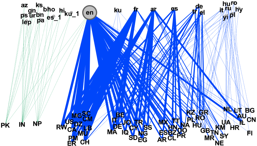
(a) Two 6-wings for $q=en$.

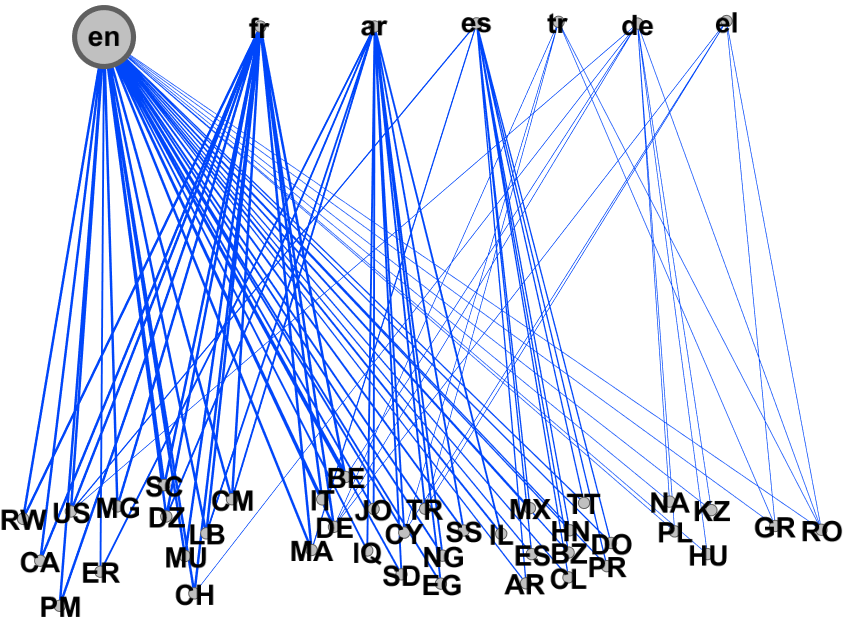
(b) One 7-wing for $q=en$.

Figure 10: k-wings in Unicode Language datasets.

The existing works in cohesive subgraph retrieval can be divided into the following sets.

Bipartite cohesive subgraphs detection. In this set of work, the problem focuses on enumerating all the cohesive subgraphs in a bipartite graph. Recently, the bipartite graph decomposition has attracted a lot of attention from the researchers [DBLP:conf/wsdm/SariyuceP18, zou2016bitruss, DBLP:conf/icde/Wang0Q0020], which can be used for querying cohesive subgraphs. Even though [Sanei-Mehri:2018:BCB:3219819.3220097, DBLP:journals/pvldb/WangLQZZ19], have improved the decomposition algorithm by improving the butterfly counting, yet they are inefficient for repetitive query processing. [liu2020efficient] presented an index-based approach to enumerate all the $(\alpha,\beta)$-core structures in a bipartite graph. The $(k,P)$-Bitruss model for the bipartite graph was also proposed in [yang2020effective] to determine the densely connected vertex of the same type. Recently, Yixiang [fang2020effective] proposed a community search (or cohesive subgraph search) in heterogeneous networks based on $(k,P)$-core structure, where $P$ is the meta path and $k$ is the minimum degree of a vertex, connected via meta path in the community. The dynamic maintenance of the index for cohesive subgraph search has been discussed in [liu2020efficient].
Cohesive subgraphs search. The cohesive subgraph search has been implemented using different distinct cohesive structures such as $k$-core [Sozio2010cocktail], $k$-truss [huang2014querying, akbas2017truss], and $\gamma$-quasi-$k$-clique [cui2014local], etc. However, all of them are from the field of unipartite graphs. Unfortunately, there have are very few such cohesive subgraph search models for bipartite graphs. Recently, [fang2020effective] proposed a community search in heterogeneous networks based on $(k,P)$-core structure, where $P$ is the meta path and $k$ is the minimum degree of a vertex, connected via meta path in the community. The resulting community search requires an extra parameter $P$ and it results in the weak cohesive community as the length of the path increases. Moreover, the resulting community only includes vertices of the same type rather than the edges from the graph, hence an overhead occurs if we want to inquire about other interests apart from the meta path. The dynamic maintenance algorithms for core number in graphs are proposed in [sariyuce2016incremental, zhang2017fast].

VII Conclusion

In this paper, we examined the problem of wing-based personalized bipartite cohesive subgraph search for large bipartite graphs. We proposed two indexing schemes EquiWing and EquiWing-Comp to tackle the problem efficiently, which leads to a linear time search algorithm. The $k$-butterfly equivalence successfully summarized the bipartite graph into EquiWing without losing any edges. Also, we constructed EquiWing-Comp by proposing the $k$-butterfly loose connectivity and exploiting the hierarchy property of a k-wing, which further speeds up the query processing. We have also discussed the efficient maintenance of the proposed indices in dynamic bipartite graphs. Moreover, we have conducted extensive experiments across large real-world datasets. From these experiments, we observe the validation of compression and performance of EquiWing-Comp over EquiWing. A case study is also presented to display the effectiveness of our $k$-wing bipartite cohesive subgraph model.