Minimizing $L_{1}$ over $L_{2}$ norms on the gradient

Abstract

In this paper, we study the $L_{1}/L_{2}$ minimization on the gradient for imaging applications. Several recent works have demonstrated that $L_{1}/L_{2}$ is better than the $L_{1}$ norm when approximating the $L_{0}$ norm to promote sparsity. Consequently, we postulate that applying $L_{1}/L_{2}$ on the gradient is better than the classic total variation (the $L_{1}$ norm on the gradient) to enforce the sparsity of the image gradient. To verify our hypothesis, we consider a constrained formulation to reveal empirical evidence on the superiority of $L_{1}/L_{2}$ over $L_{1}$ when recovering piecewise constant signals from low-frequency measurements. Numerically, we design a specific splitting scheme, under which we can prove subsequential and global convergence for the alternating direction method of multipliers (ADMM) under certain conditions. Experimentally, we demonstrate visible improvements of $L_{1}/L_{2}$ over $L_{1}$ and other nonconvex regularizations for image recovery from low-frequency measurements and two medical applications of MRI and CT reconstruction. All the numerical results show the efficiency of our proposed approach.

Keywords: $L_{1}/L_{2}$ minimization, piecewise constant images, minimum separation, alternating direction method of multipliers

1 Introduction

Regularization methods play an important role in inverse problems to refine the solution space by prior knowledge and/or special structures. For example, the celebrated total variation (TV) [1] prefers piecewise constant images, while total generalized variation (TGV) [2] and fractional-order TV [3, 4] tend to preserve piecewise smoothness of an image. TV can be defined either isotropically or anisotropically. The anisotropic TV [5] in the discrete setting is equivalent to applying the $L_{1}$ norm on the image gradient. As the $L_{1}$ norm is often used to enforce a signal being sparse, one can interpret the TV regularization as to promote the sparsity of gradient vectors.

To find the sparsest signal, it is straightforward to minimize the $L_{0}$ norm (counting the number of nonzero elements), which is unfortunately NP-hard [6]. A popular approach involves the convex relaxation of using the $L_{1}$ norm to replace the ill-posed $L_{0}$ norm, with the equivalence between $L_{1}$ and $L_{0}$ for sparse signal recovery given in terms of restricted isometry property (RIP) [7]. However, Fan and Li [8] pointed out that the $L_{1}$ approach is biased towards large coefficients, and proposed to minimize a nonconvex regularization, called smoothly clipped absolute deviation (SCAD). Subsequently, various nonconvex functionals emerged such as minimax concave penalty (MCP) [9], capped $L_{1}$ [10, 11, 12], and transformed $L_{1}$ [13, 14, 15]. Following the literature on sparse signal recovery, there is a trend to apply a nonconvex regularization on the gradient to deal with images. For instance, Chartrand [16] discussed both the $L_{p}$ norm with $0<p<1$ for sparse signals and $L_{p}$ on the gradient for magnetic resonance imaging (MRI), while MCP on the gradient was proposed in [17].

Recently, a scale-invariant functional $L_{1}/L_{2}$ was examined, which gives promising results in recovering sparse signals [18, 19, 20] and sparse gradients [21]. In this paper, we rely on a constrained formulation to characterize some scenarios, under which the quotient of the $L_{1}$ and $L_{2}$ norms on the gradient performs well. In particular, we borrow the analysis of a super-resolution problem, which refers to recovering a sparse signal from its low-frequency measurements. Candés and Fernandez-Granda [22] proved that if a signal has spikes (locations of nonzero elements) that are sufficiently separated, then the $L_{1}$ minimization yields an exact recovery for super-resolution. We innovatively design a certain type of piecewise constant signals that lead to well-separated spikes after taking the gradient. Using such signals, we empirically demonstrate that the TV minimization can find the desired solution under a similar separation condition as in [22]. We also illustrate that $L_{1}/L_{2}$ can deal with less separated spikes in gradient, and is better at preserving image contrast than $L_{1}$. These empirical evidences show $L_{1}/L_{2}$ holds great potentials in promoting sparse gradients and preserving image contrasts. To the best of our knowledge, it is the first time to relate the exact recovery of gradient-based methods to minimum separation and image contrast in a super-resolution problem.

Numerically, we consider the same splitting scheme used in an unconstrained formulation [21] to minimize the $L_{1}/L_{2}$ on the gradient, followed by the alternating direction method of multipliers (ADMM) [23]. We formulate the linear constraint using an indicator function, which is not strongly convex. As a result, the convergence analysis in the unconstrained model [21] is not directly applicable to this problem. We utilize the property of indicator function as well as the optimality conditions for constrained optimization problems to prove that the sequence generated by the proposed algorithm has a subsequence converging to a stationary point. Under a stronger assumption, we can establish the convergence of the entire sequence, referred to as global convergence.

We present some algorithmic insights on computational efficiency of our proposed algorithm for nonconvex optimization. In particular, we show an additional box constraint not only prevents the solution from being stuck at local minima, but also stabilizes the algorithm. Furthermore, we discuss algorithmic behaviors on two types of applications: MRI and computed tomography (CT). For the MRI reconstruction, a subproblem in ADMM has a closed-form solution, while an iterative solver is required for CT. As the accuracy of the subproblem varies between MRI and CT, we shall alter internal settings of our algorithm accordingly. In summary, this paper relies on a constrained formulation to discuss theoretical and computational aspects of a nonconvex regularization for imaging problems. The major contributions are three-fold:

1. We reveal empirical evidences towards exact recovery of piecewise constant signals and demonstrate the superiority of $L_{1}/L_{2}$ on the gradient over TV.

2. We establish the subsequential convergence of the proposed algorithm and explore the global convergence under the certain assumptions.

3. We conduct extensive experiments to characterize computational efficiency of our algorithm and discuss how internal settings can be customized to cater to specific imaging applications, such as MRI and limited-angle CT reconstruction. Numerical results highlight the superior performance of our approach over other gradient-based regularizations.

The rest of the paper is organized as follows. Section 2 defines the notations that will be used through the paper, and gives a brief review on the related works. The empirical evidences for TV’s exact recovery and advantages of the proposed model are given in Section 3. The numerical scheme is detailed in Section 4, followed by convergence analysis in Section 5. Section 6 presents three types of imaging applications: super-resolution, MRI and CT reconstruction problems. Finally, conclusions and future works are given in Section 7.

2 Preliminaries

We use a bold letter to denote a vector, a capital letter to denote a matrix or linear operator, and a calligraphic letter for a functional space. We use $\odot$ to denote the component-wise multiplication of two vectors. When a function (e.g., sign, max, min) applies to a vector, it returns a vector with corresponding component-wise operation.

We adopt a discrete setting to describe the related models. Suppose a two-dimensional (2D) image is defined on an $m\times n$ Cartesian grid. By using a standard linear index, we can represent a 2D image as a vector, i.e., the $((i-1)m+j)$-th component denotes the intensity value at pixel $(i,j).$ We define a discrete gradient operator,

$$D\mathbf{u}:=\left[\begin{array}[]{l}D_{x}\\ D_{y}\end{array}\right]\mathbf{u},$$ (1)

where $D_{x},D_{y}$ are the finite forward difference operator with periodic boundary condition in the horizontal and vertical directions, respectively. We denote $N:=mn$ and the Euclidean spaces by $\mathcal{X}:=\mathds{R}^{N},\mathcal{Y}:=\mathds{R}^{2N}$, then $\mathbf{u}\in\mathcal{X}$ and $D\mathbf{u}\in\mathcal{Y}$. We can apply the standard norms, e.g., $L_{1},L_{2},$ on vectors $\mathbf{u}$ and $D\mathbf{u}.$ For example, the $L_{1}$ norm on the gradient, i.e., $\|D\mathbf{u}\|_{1}$, is the anisotropic TV regularization [5]. Throughout the paper, we use TV and “$L_{1}$ on the gradient” interchangeably. Note that the isotropic TV [1] is the $L_{2,1}$ norm, i.e., $\|(D_{x}\mathbf{u},D_{y}\mathbf{u})^{T}\|_{2,1},$ although Lou et al. [24] claimed to consider a weighted difference of anisotropic and isotropic TV based on the $L_{1}$-$L_{2}$ functional [25, 26, 27, 28] (isotropic TV is not the $L_{2}$ norm on the gradient.)

We examine the $L_{1}/L_{2}$ penalty on the gradient in a constrained formulation,

$$\min_{\mathbf{u}}\frac{\|D\mathbf{u}\|_{1}}{\|D\mathbf{u}\|_{2}}\quad\mathrm{s.t.}\ \ A\mathbf{u}=\mathbf{b}.$$ (2)

One way to solve for (2) involves the following equivalent form

$$\min_{\mathbf{u},\mathbf{d},\mathbf{h}}\frac{\|\mathbf{d}\|_{1}}{\|\mathbf{h}\|_{2}}\quad\mathrm{s.t.}\ \ A\mathbf{u}=\mathbf{b},\ \mathbf{d}=D\mathbf{u},\ \mathbf{h}=D\mathbf{u},$$ (3)

with two auxiliary variables $\mathbf{d}$ and $\mathbf{h}$. For more details, please refer to [18] that presented a proof-of-concept example for MRI reconstruction. Since the splitting scheme (3) involves two block variables of $\mathbf{u}$ and $(\mathbf{d},\mathbf{h})$, the existing ADMM convergence results [29, 30, 31] are not applicable. An alternative approach was discussed in our preliminary work [21] for an unconstrained minimization problem,

$$\min_{\mathbf{u},\mathbf{h}}\frac{\|D\mathbf{u}\|_{1}}{\|\mathbf{h}\|_{2}}+\frac{\lambda}{2}\|A\mathbf{u}-\mathbf{b}\|_{2}^{2}\quad\mathrm{s.t.}\quad\mathbf{h}=D\mathbf{u},$$ (4)

where $\lambda>0$ is a weighting parameter. By only introducing one variable $\mathbf{h},$ the new splitting scheme (4) can guarantee the ADMM framework with subsequential convergence.

In this paper, we incorporate the splitting scheme (4) to solve the constrained problem (2), which is crucial to reveal theoretical properties of the gradient-based regularizations for image reconstruction, as elaborated in Section 3. Another contribution of this work lies in the convergence analysis, specifically for different optimality conditions of the constrained problem, as opposed to unconstrained formulation presented in [21]. It is true that the constrained formulation limits our experimental design in a noise-free fashion, but it helps us to draw conclusions solely on the model, ruling out the influence from other nuisances such as noises and tuning parameters. Our model (2) is parameter-free, while there is a parameter $\lambda$ in the unconstrained problem (4).

3 Empirical studies

We aim to demonstrate the superiority of $L_{1}/L_{2}$ on the gradient over TV for a super-resolution problem [32], in which a sparse vector can be exactly recovered via the $L_{1}$ minimization. A mathematical model for super-resolution is expressed as

$$b_{k}=\frac{1}{\sqrt{N}}\sum_{j=0}^{N-1}u_{j}e^{-i2\pi kj/N},\qquad|k|\leq f_{c},$$ (5)

where $i$ is the imaginary unit, $\mathbf{u}\in\mathbb{R}^{N}$ is a vector to be recovered, and $\mathbf{b}\in\mathbb{C}^{n}$ consists of the given low frequency measurements with $n=2f_{c}+1<N$. Recovering $\mathbf{u}$ from $\mathbf{b}$ is referred to as super-resolution in the sense that the underlying signal $\mathbf{u}$ is defined on a fine grid with spacing $1/N$, while a direct inversion of $n$ frequency data yields a signal defined on a coarser grid with spacing $1/n$. For simplicity, we use matrix notation to rewrite (5) as $\mathbf{b}=S_{n}F\mathbf{u}$, where $S_{n}$ is a sampling matrix that collects the required low frequencies and $F$ is the Fourier transform matrix. A sparse signal can be represented by $\mathbf{u}=\sum_{j\in T}c_{j}\mathbf{e}_{j},$ where $\mathbf{e}_{j}$ is the $j$-th canonical basis in $\mathbb{R}^{N}$, $T$ is the support set of $\mathbf{u}$, and $\{c_{j}\}$ are coefficients. Following the work of [32], the sparse spikes are required to be sufficiently separated to guarantee the exact recovery of the $L_{1}$ minimization. To make the paper self-contained, we provide the definition of minimum separation in Definition 1 and an exact recovery condition in Theorem 1.

Definition 1.

(Minimum Separation [32]) For an index set $T\subset\{1,\cdots,N\}$, the minimum separation (MS) of $T$ is defined as the closest wrap-around distance between any two elements from $T$,

$$\triangle(T):=\min_{(t,\tau)\in T:t\neq\tau}\min\left\{|t-\tau|,\ N-|t-\tau|\right\}.$$ (6)

Theorem 1.

[32, Corollary 1.4] Let $T$ be the support of $\mathbf{u}$. If the minimum separation of $T$ obeys

$$\triangle(T)\geq\frac{1.87N}{f_{c}},$$ (7)

then $\mathbf{u}\in\mathbb{R}^{N}$ is the unique solution to the constrained $L_{1}$ minimization problem,

$$\min_{\mathbf{u}}\|\mathbf{u}\|_{1}\quad\mbox{\rm s.t.}\quad S_{n}F\mathbf{u}=\mathbf{b}.$$ (8)

We empirically extend the analysis from sparse signals to sparse gradients. For this purpose, we construct a one-bar step function of length 100 with the first and the last $s$ elements taking value 0, and the remaining elements equal to 1, as illustrated in Figure 1. The gradient of such signal is 2-sparse with MS to be $\min(2s,100-2s)$ due to wrap-around distance. By setting $f_{c}=2,$ we only take $n=5$ low frequency measurements, and reconstruct the signal by minimizing either $L_{1}$ or $L_{1}/L_{2}$ on the gradient. For simplicity, we adopt the CVX MATLAB toolbox [33] for solving the TV model,

$$\min_{\mathbf{u}}\|D\mathbf{u}\|_{1}\quad\mathrm{s.t.}\quad A\mathbf{u}=\mathbf{b},$$ (9)

where we use $A=S_{n}F$ to be consistent with our setting (2). Note that the TV model (9) is parameter free, while we need to tune an algorithmic parameter for $L_{1}/L_{2}$. Please refer to Section 4 for more details on the $L_{1}/L_{2}$ minimization, in which one subproblem can be solved by CVX, and Section 6.1 for sensitivity analysis on this parameter.

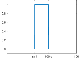
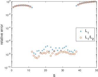
Figure 1: A general setting of a one-bar step function (left) and reconstruction errors with respect to $s$ (right) by minimizing $L_{1}$ or $L_{1}/L_{2}$ on the gradient. The exact recovery interval by $L_{1}$ is $s\in[13,37],$ which is smaller than $[12,38]$ by $L_{1}/L_{2}.$

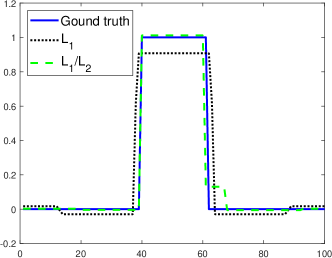
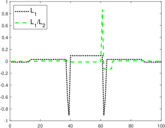
Figure 2: A particular one-bar example (left) where both $L_{1}$ and $L_{1}/L_{2}$ models fail to find the solution. The different plot (right) highlights that $L_{1}$ results in larger oscillations compared to $L_{1}/L_{2}.$

By varying the value of $s$ that changes MS of the spikes in gradient, we compute the relative errors between the reconstructed solutions and the ground-truth signals. If we define an exact recovery for its relative error smaller than $10^{-6}$, we observe in Figure 1 that the exact recovery by $L_{1}$ occurs at $s\in[13,37],$ which implies that MS is larger than or equal to $26$. This phenomenon suggests that Theorem 1 might hold for sparse gradients by replacing the $L_{1}$ norm with the total variation. Figure 1 also shows the exact recovery by $L_{1}/L_{2}$ at $s\in[12,38],$ meaning that $L_{1}/L_{2}$ can deal with less separated spikes than $L_{1}$. Moreover, we further study the reconstruction results at $s=39,$ where both models fail to find the true sparse signal. The restored solutions by these two models as well as the different plots between restored and ground truth are displayed in Figure 2, showing that our ratio model has smaller relative errors than $L_{1}$.

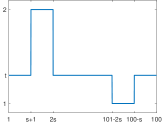
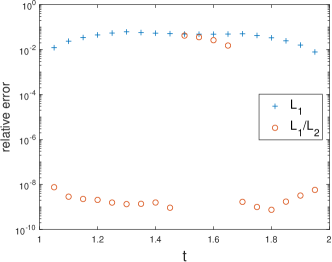
Figure 3: A general setting of a two-bar step function (left) and reconstruction errors with respect to $t$ (right) by minimizing $L_{1}$ or $L_{1}/L_{2}$ on the gradient, showing that $L_{1}/L_{2}$ is better at preserving image contrast than $L_{1}$ (controlled by $t$).

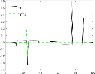
Figure 4: A particular two-bar example where both $L_{1}$ and $L_{1}/L_{2}$ models fail to find the solution. The different plot is shown on the right.

Figure 2 illustrates that the TV solution can not reach the top of the bar in the ground-truth, which is referred to as loss-of-contrast. Motivated by this well-known drawback of TV, we postulate that the signal contrast may affect the performance of $L_{1}$ and $L_{1}/L_{2}$. To verify, we examine a two-bar step function, in which the contrast varies by the relative heights of the two bars. Following MATLAB’s notation, we set $\mathbf{u}(s+1:2s)=2,\mathbf{u}(\text{end}-2s+1:\text{end})=1,$ and the value of remaining elements uniformly as $t$; see Figure 3 for a general setting. We fix $s=12$, and vary the value of $t\in(1,2)$ to generate signals with different intensity contrasts. Considering four spikes in the gradient, we set $f_{c}=4$ or equivalently 9 low-frequency measurements to reconstruct the signal. The reconstruction errors are plotted in Figure 3, which shows that $L_{1}$ fails in all the cases, and $L_{1}/L_{2}$ can find the signals except for $t\in[1.5,1.65]$. We further examine a particular case of $t=1.65$ in Figure 4, where both models fail to get an exact recovery, but $L_{1}/L_{2}$ yields smaller oscillations than $L_{1}$ near the edges. Figures 3 and 4 demonstrate that $L_{1}/L_{2}$ is better at preserving image contrast than $L_{1}$.

We verify that all the solutions of $L_{1}$ and $L_{1}/L_{2}$ satisfy the linear constraint $A\mathbf{u}=\mathbf{b}$ with high accuracy thanks for CVX. We further investigate when the $L_{1}$ approach fails, and discover that it yields a solution that has a smaller $L_{1}$ norm compared to the $L_{1}$ norm of the ground-truth, which implies that $L_{1}$ is not sufficient to enforce gradient sparse. On the other hand, $L_{1}/L_{2}$ solutions often have higher objective value than the ground-truth, which calls for a better algorithm that can potentially find the ground-truth. We also want to point out that $L_{1}/L_{2}$ solutions depend on initial conditions. In Figure 1 and Figure 3, we present the smallest relative errors among 10 random vectors for initial values.

The minimum separation distance in 1D (Definition 1) can be naturally extended to 2D. In fact, there are two types of minimum separation definitions in 2D: one uses the $L_{\infty}$ norm to measure the distance [32], while another definition is called Rayleigh regularity [34, 35]. The exact recovery for 2D sparse vectors was characterized in [35] with additional restriction of positive signals. Both distance definitions were empirically examined in [12] for point-source super-resolution. When extending to 2D sparse gradient, one can compute the gradient norm at each pixel, and separation distance can be defined as the distance between any two locations with non-zero gradient norm. To the best of our knowledge, there is no analysis on the exact recovery of sparse gradients, no matter whether it is in 1D or 2D. In Section 3, we devote some empirical evidences, showing a similar relationship between sparse gradient recovery and minimum separation as Theorem 1, which calls for a theoretical justification in the future. Once the extension from 1D sparse vectors to 1D sparse gradients is established, it is expected that the analysis can be applied to sparse gradients in 2D to facilitate theoretical analysis in imaging applications.

4 The proposed approach

Starting from (2), we incorporate an additional box constraint in the model, i.e.,

$$\min_{\mathbf{u}}\frac{\|D\mathbf{u}\|_{1}}{\|D\mathbf{u}\|_{2}}\quad\mathrm{s.t.}\quad A\mathbf{u}=\mathbf{b},\ \mathbf{u}\in{\color[rgb]{0,0,0}[p,q]^{N}}.$$ (10)

The notation $\mathbf{u}\in[p,q]^{N}$ means that every element of $\mathbf{u}$ is bounded by $[p,q].$ The box constraint is reasonable for image processing applications [36, 37], since pixel values are usually bounded by $[0,1]$ or $[0,255]$. On the other hand, the box constraint is particularly helpful for the $L_{1}/L_{2}$ model to prevent its divergence [19].

We use the indicator function to rewrite (10) into the following equivalent form

$$\min_{\mathbf{u},\mathbf{h}}\frac{\|D\mathbf{u}\|_{1}}{\|\mathbf{h}\|_{2}}+\Pi_{A\mathbf{u}=\mathbf{b}}(\mathbf{u})+\Pi_{{\color[rgb]{0,0,0}[p,q]^{N}}}(\mathbf{u})\quad\mathrm{s.t.}\quad D\mathbf{u}=\mathbf{h},$$ (11)

where $\Pi_{S}(\mathbf{t})$ denotes the indicator function that forces $\mathbf{t}$ to belong to a feasible set $S$, i.e.,

$$\Pi_{S}(\mathbf{t})=\begin{cases}0&\mbox{if }\mathbf{t}\in S\\ +\infty&\text{otherwise}.\end{cases}$$ (12)

The augmented Lagrangian function corresponding to (11) can be expressed as,

$$\mathcal{L}(\mathbf{u},\mathbf{h};\mathbf{g})=\frac{\|D\mathbf{u}\|_{1}}{\|\mathbf{h}\|_{2}}+\Pi_{A\mathbf{u}=\mathbf{b}}(\mathbf{u})+\Pi_{[p,q]^{N}}(\mathbf{u})+\langle\rho\mathbf{g},D\mathbf{u}-\mathbf{h}\rangle+\frac{\rho}{2}\|D\mathbf{u}-\mathbf{h}\|_{2}^{2},$$ (13)

where $\mathbf{g}$ is a dual variable and $\rho$ is a positive parameter. Then ADMM iterates as follows,

$$\left\{\begin{array}[]{l}\mathbf{u}^{(k+1)}=\arg\min_{\mathbf{u}}\mathcal{L}(\mathbf{u},\mathbf{h}^{(k)};\mathbf{g}^{(k)})\\ \mathbf{h}^{(k+1)}=\arg\min_{\mathbf{h}}\mathcal{L}(\mathbf{u}^{(k+1)},\mathbf{h};\mathbf{g}^{(k)})\\ \mathbf{g}^{(k+1)}=\mathbf{g}^{(k)}+D\mathbf{u}^{(k+1)}-\mathbf{h}^{(k+1)}.\end{array}\right.$$ (14)

The update for $\mathbf{h}$ is the same as in [18], which has a closed-form solution of

$$\mathbf{h}^{(k+1)}=\begin{cases}\tau^{(k)}(D\mathbf{u}^{(k+1)}+\mathbf{g}^{(k)})&\mbox{if }D\mathbf{u}^{(k+1)}+\mathbf{g}^{(k)}\neq\mathbf{0}\\ \mathbf{r}^{(k)}&\text{otherwise},\end{cases}$$ (15)

where $\mathbf{r}^{(k)}$ is a random vector with the $L_{2}$ norm being $\sqrt[3]{\frac{\|D\mathbf{u}^{(k+1)}\|_{1}}{\rho}}$ and $\tau^{(k)}=\frac{1}{3}+\frac{1}{3}(\xi^{(k)}+\frac{1}{\xi^{(k)}})$ for

$$\xi^{(k)}=\sqrt[3]{\frac{27\eta^{(k)}+2+\sqrt{(27\eta^{(k)}+2)^{2}-4}}{2}}\quad\mbox{and}\quad\eta^{(k)}=\frac{\|D\mathbf{u}^{(k+1)}\|_{1}}{\rho\|D\mathbf{u}^{(k+1)}+\mathbf{g}^{(k)}\|_{2}^{3}}.$$

We elaborate on the $\mathbf{u}$-subproblem in (14), which can be expressed by the box constraint, i.e.,

$$\mathbf{u}^{(k+1)}=\arg\min_{\mathbf{u}}\frac{\|D\mathbf{u}\|_{1}}{\|\mathbf{h}^{(k)}\|_{2}}+\frac{\rho}{2}\|D\mathbf{u}-\mathbf{h}^{(k)}+\mathbf{g}^{(k)}\|_{2}^{2}\quad\mathrm{s.t.}\quad A\mathbf{u}=\mathbf{b},\mathbf{u}\in[p,q]^{N}.$$ (16)

To solve for (16), we introduce two variables, $\mathbf{v}$ for the box constraint and $\mathbf{d}$ for the gradient, thus getting

$$\min_{\mathbf{u},\mathbf{d},\mathbf{v}}\frac{\|\mathbf{d}\|_{1}}{\|\mathbf{h}^{(k)}\|_{2}}+\frac{\rho}{2}\|D\mathbf{u}-\mathbf{h}^{(k)}+\mathbf{g}^{(k)}\|_{2}^{2}+\Pi_{{\color[rgb]{0,0,0}[p,q]^{N}}}(\mathbf{v})\quad\mathrm{s.t.}\quad\mathbf{u}=\mathbf{v},D\mathbf{u}=\mathbf{d},A\mathbf{u}=\mathbf{b}.$$ (17)

The augmented Lagrangian function corresponding to (17) becomes

$$\begin{split}\mathcal{L}^{(k)}(\mathbf{u},\mathbf{d},\mathbf{v};\mathbf{w},\mathbf{y},\mathbf{z})=&\frac{\|\mathbf{d}\|_{1}}{\|\mathbf{h}^{(k)}\|_{2}}+\frac{\rho}{2}\|D\mathbf{u}-\mathbf{h}^{(k)}+\mathbf{g}^{(k)}\|_{2}^{2}+\Pi_{{\color[rgb]{0,0,0}[p,q]^{N}}}(\mathbf{v})\\ &+\langle\beta\mathbf{w},\mathbf{u}-\mathbf{v}\rangle+\frac{\beta}{2}\|\mathbf{u}-\mathbf{v}\|_{2}^{2}\\ &+\langle\gamma\mathbf{y},D\mathbf{u}-\mathbf{d}\rangle+\frac{\gamma}{2}\|D\mathbf{u}-\mathbf{d}\|_{2}^{2}\\ &+\langle\lambda\mathbf{z},A\mathbf{u}-\mathbf{b}\rangle+\frac{\lambda}{2}\|A\mathbf{u}-\mathbf{b}\|_{2}^{2},\end{split}$$ (18)

where $\mathbf{w},\mathbf{y},\mathbf{z}$ are dual variables and $\beta,\gamma,\lambda$ are positive parameters. Here we have $k$ in the superscript of $\mathcal{L}$ to indicate that it is the Lagrangian for the $\mathbf{u}$-subproblem in (14) at the $k$-th iteration. The ADMM framework to minimize (17) leads to

$$\left\{\begin{array}[]{l}\mathbf{u}_{j+1}=\arg\min_{\mathbf{u}}\mathcal{L}^{(k)}(\mathbf{u},\mathbf{d}_{j},\mathbf{v}_{j};\mathbf{w}_{j},\mathbf{y}_{j},\mathbf{z}_{j})\\ \mathbf{d}_{j+1}=\arg\min_{\mathbf{d}}\mathcal{L}^{(k)}(\mathbf{u}_{j+1},\mathbf{d},\mathbf{v}_{j};\mathbf{w}_{j},\mathbf{y}_{j},\mathbf{z}_{j})\\ \mathbf{v}_{j+1}=\arg\min_{\mathbf{v}}\mathcal{L}^{(k)}(\mathbf{u}_{j+1},\mathbf{d}_{j+1},\mathbf{v};\mathbf{w}_{j},\mathbf{y}_{j},\mathbf{z}_{j})\\ \mathbf{w}_{j+1}=\mathbf{w}_{j}+\mathbf{u}_{j+1}-\mathbf{v}_{j+1}\\ \mathbf{y}_{j+1}=\mathbf{y}_{j}+D\mathbf{u}_{j+1}-\mathbf{d}_{j+1}\\ \mathbf{z}_{j+1}=\mathbf{z}_{j}+A\mathbf{u}_{j+1}-\mathbf{b},\end{array}\right.$$ (19)

where the subscript $j$ represents the inner loop index, as opposed to the superscript $k$ for outer iterations in (14). By taking derivative of $\mathcal{L}^{(k)}$ with respect to $\mathbf{u}$, we obtain a closed-form solution given by

$$\begin{split}\mathbf{u}_{j+1}&=\Big{(}\lambda A^{T}A+(\rho+\gamma)D^{T}D+\beta I\Big{)}^{-1}\Big{(}\lambda A^{T}(\mathbf{b}-\mathbf{z}_{j})\\ &\quad+\gamma D^{T}(\mathbf{d}_{j}-\mathbf{y}_{j})+\rho D^{T}(\mathbf{h}^{(k)}-\mathbf{g}^{(k)})+\beta(\mathbf{v}_{j}-\mathbf{w}_{j})\Big{)},\end{split}$$ (20)

where $I$ stands for the identity matrix. When the matrix $A$ involves frequency measurements, e.g. in super-resolution and MRI reconstruction, the update in (20) can be implemented efficiently by the fast Fourier transform (FFT) for periodic boundary conditions when defining the derivative operator $D$ in (1). For a general system matrix $A$, we adopt the conjugate gradient descent iterations [38] to solve for (20).

The $\mathbf{d}$-subproblem in (19) also has a closed-form solution, i.e.,

$$\mathbf{d}_{j+1}=\mathbf{shrink}\left(D\mathbf{u}_{j+1}+\mathbf{y}_{j},\frac{1}{\gamma\|\mathbf{h}^{(k)}\|_{2}}\right),$$ (21)

where $\mathbf{shrink}(\mathbf{x},\mu)=\mathrm{sign}(\mathbf{x})\odot\max\left\{|\mathbf{x}|-\mu,0\right\}$ is called soft shrinkage and $\odot$ denotes element-wise multiplication. We update $\mathbf{v}$ by a projection onto the $[p,q]$-box constraint, which is given by

$$\mathbf{v}_{j+1}=\min\left\{\max\{\mathbf{u}_{j+1}+\mathbf{w}_{j},p\},q\right\}.$$

In summary, we present an ADMM-based algorithm to minimize the $L_{1}/L_{2}$ on the gradient subject to a linear system with the box constraint in Algorithm 1. If we only run one iteration of the $\mathbf{u}$-subproblem (19), the overall ADMM iteration (14) is equivalent to the previous approach [18].

Algorithm 1 The $L_{1}/L_{2}$ minimization on the gradient

1:  Input: a linear operator $A$, observed data $\mathbf{b}$, and a bound $[p,q]$ for the original image

2:  Parameters: $\rho,\lambda,\gamma,\beta$, kMax, jMax, and $\epsilon\in\mathds{R}$

3:  Initialize: $\mathbf{h},\mathbf{d},\mathbf{g},\mathbf{v},\mathbf{w},\mathbf{y},\mathbf{z}=\mathbf{0}$, and $k,j=0$

4:  while $k<$ kMax or $\|\mathbf{u}^{(k)}-\mathbf{u}^{(k-1)}\|_{2}/\|\mathbf{u}^{(k)}\|_{2}>\epsilon$ do

5:     while $j<$ jMax or $\|\mathbf{u}_{j}-\mathbf{u}_{j-1}\|_{2}/\|\mathbf{u}_{j}\|_{2}>\epsilon$ do

6:        $\mathbf{u}_{j+1}=(\lambda A^{T}A+(\rho+\gamma)D^{T}D+\beta I)^{-1}(\lambda A^{T}(\mathbf{b}-\mathbf{z}_{j})+\gamma D^{T}(\mathbf{d}_{j}-\mathbf{y}_{j})$ $\quad\quad\quad+\rho D^{T}(\mathbf{h}^{(k)}-\mathbf{g}^{(k)})+\beta(\mathbf{v}_{j}-\mathbf{w}_{j}))$

7:        $\mathbf{d}_{j+1}=\mathbf{shrink}\left(D\mathbf{u}_{j+1}+\mathbf{y}_{j},\frac{1}{\gamma\|\mathbf{h}^{(k)}\|_{2}}\right)$

8:        $\mathbf{v}_{j+1}=\min\left\{\max\{\mathbf{u}_{j+1}+\mathbf{w}_{j},p\},q\right\}$

9:        $\mathbf{w}_{j+1}=\mathbf{w}_{j}+\mathbf{u}_{j+1}-\mathbf{v}_{j+1}$

10:        $\mathbf{y}_{j+1}=\mathbf{y}_{j}+D\mathbf{u}_{j+1}-\mathbf{d}_{j+1}$

11:        $\mathbf{z}_{j+1}=\mathbf{z}_{j}+A\mathbf{u}_{j+1}-\mathbf{b}$

12:        $j=j+1$

13:     end while

14:     return  $\mathbf{u}^{(k+1)}=\mathbf{u}_{j}$

15:     Update $\mathbf{h}^{(k+1)}$ by (15).

16:     $\mathbf{g}^{(k+1)}=\mathbf{g}^{(k)}+D\mathbf{u}^{(k+1)}-\mathbf{h}^{(k+1)}$

17:     $k=k+1$ and $j=0$

18:  end while

19:  return  $\mathbf{u}^{\ast}=\mathbf{u}^{(k)}$

5 Convergence analysis

We intend to establish the convergence of Algorithm 1 with the box constraint, which is extensively tested in the experiments. Since our ADMM framework (14) share the same structure with the unconstrained formulation, we adapt some analysis in [21] to prove the subsequential convergence for the proposed model (10). For example, we make the same assumptions as in [21],

Assumption 1.

${\cal N}(D)\bigcap{\cal N}(A)=\{\mathbf{0}\}$, where $\cal N$ denotes the null space and $D$ is defined in (1). In addition, the norm of $\{\mathbf{h}^{(k)}\}$ generated by (14) has a lower bound, i.e., there exists a positive constant $\epsilon$ such that $\|\mathbf{h}^{(k)}\|_{2}\geq\epsilon,\ \forall k$.

Remark 1.

We have $\|\mathbf{h}\|_{2}>0$ in the $L_{1}/L_{2}$ model as the denominator shall not be zero. It is true that $\|\mathbf{h}\|_{2}>0$ does not imply a uniform lower bound of $\epsilon$ such that $\|\mathbf{h}\|_{2}>\epsilon$ in Assumption 1. Here we can redefine the divergence of an algorithm by including the case of $\|\mathbf{h}^{(k)}\|_{2}<\epsilon$, which can be checked numerically with a pre-set value of $\epsilon$.

Unlike the unconstrained model (4), the strong convexity of $\mathcal{L}(\mathbf{u},\mathbf{h},\mathbf{g})$ with respect to $\mathbf{u}$ does not hold due to the indicator function $\Pi_{A\mathbf{u}=\mathbf{b}}(\mathbf{u})$. Besides, we have additional dual variable $\mathbf{w}$ which is not in the unconstrained model. To avoid redundancies to [21], we focus on the different strategies to the unconstrained case, such as optimality conditions and subgradient of the indicator function, when proving convergence for the constrained problem, e.g., in Lemmas 1-2 and Theorem 2.

Lemma 1.

(sufficient descent) Under 1, the sequence $\{\mathbf{u}^{(k)},\mathbf{h}^{(k)},\mathbf{g}^{(k)}\}$ generated by (14) satisfies

$$\mathcal{L}(\mathbf{u}^{(k+1)},\mathbf{h}^{(k+1)};\mathbf{g}^{(k+1)})\leq\mathcal{L}(\mathbf{u}^{(k)},\mathbf{h}^{(k)};\mathbf{g}^{(k)})-c_{1}\|\mathbf{u}^{(k+1)}-\mathbf{u}^{(k)}\|_{2}^{2}-c_{2}\|\mathbf{h}^{(k+1)}-\mathbf{h}^{(k)}\|_{2}^{2},$$ (22)

where $c_{1}$ and $c_{2}$ are two positive constants for a sufficiently large $\rho$.

Proof.

Denote $\sigma$ as the smallest eigenvalue of the matrix $A^{T}A+D^{T}D.$ We show $\sigma$ is strictly positive. If $\sigma=0,$ there exists a nonzero vector $\mathbf{x}$ such that $\mathbf{x}^{T}(A^{T}A+D^{T}D)\mathbf{x}=0$. It is straightforward that $\mathbf{x}^{T}A^{T}A\mathbf{x}\geq 0$ and $\mathbf{x}^{T}D^{T}D\mathbf{x}\geq 0$, so one shall have $\mathbf{x}^{T}A^{T}A\mathbf{x}=0$ and $\mathbf{x}^{T}D^{T}D\mathbf{x}=0$, which contradicts ${\cal N}(D)\bigcap{\cal N}(A)=\{\mathbf{0}\}$ in 1. Therefore, there exists a positive $\sigma>0$ such that

$$\mathbf{v}^{T}(A^{T}A+D^{T}D)\mathbf{v}\geq\sigma\|\mathbf{v}\|_{2}^{2},\quad\forall\mathbf{v}.$$

By letting $\mathbf{v}=\mathbf{u}^{(k+1)}-\mathbf{u}^{(k)}$ and using $A\mathbf{u}^{(k+1)}=A\mathbf{u}^{(k)}=\mathbf{b}$, we have

$$\|D(\mathbf{u}^{(k+1)}-\mathbf{u}^{(k)})\|_{2}^{2}\geq\sigma\|\mathbf{u}^{(k+1)}-\mathbf{u}^{(k)}\|_{2}^{2}.$$ (23)

We express the $\mathbf{u}$-subproblem in (14) equivalently as

$$\mathbf{u}^{(k+1)}=\arg \min_{\mathbf{u}}\frac{\|D\mathbf{u}\|_{1}}{\|\mathbf{h}^{(k)}\|_{2}}+\frac{\rho}{2}\|D\mathbf{u}-\mathbf{h}^{(k)}+\mathbf{g}^{(k)}\|_{2}^{2}$$

$$\mathrm{s.t.}\quad A\mathbf{u}=\mathbf{b},p-\mathbf{u}\leq\mathbf{0},\mathrm{and}\ \mathbf{u}-q\leq\mathbf{0}.$$

The optimality conditions state that $A\mathbf{u}^{(k+1)}=\mathbf{b}$ and there exist three sets of vectors $\mathbf{w}_{i}(i=1,2,3)$ such that

$$\mathbf{0}{\color[rgb]{0,0,0}=}\frac{\mathbf{p}^{(k+1)}}{\|\mathbf{h}^{(k)}\|_{2}}+\rho D^{T}(D\mathbf{u}^{(k+1)}-\mathbf{h}^{(k)}+\mathbf{g}^{(k)})+A^{T}\mathbf{w}_{1}-\mathbf{w}_{2}+\mathbf{w}_{3},$$ (24)

with $\mathbf{p}^{(k+1)}\in\partial\|D\mathbf{u}^{(k+1)}\|_{1}$. By the complementary slackness, we have $\mathbf{w}_{2},\mathbf{w}_{3}\geq\mathbf{0}$ and

$$(p-\mathbf{u}^{(k+1)})\odot\mathbf{w}_{2}=(\mathbf{u}^{(k+1)}-q)\odot\mathbf{w}_{3}=\mathbf{0},$$ (25)

which also holds for $\mathbf{u}^{(k)}.$ Using the definition of subgradient, $A\mathbf{u}^{(k+1)}=A\mathbf{u}^{(k)}=\mathbf{b}$, and (23)-(25), we obtain that

$$\begin{split}&\mathcal{L}(\mathbf{u}^{(k+1)},\mathbf{h}^{(k)};\mathbf{g}^{(k)})-\mathcal{L}(\mathbf{u}^{(k)},\mathbf{h}^{(k)};\mathbf{g}^{(k)})\\ \leq&\langle\frac{\mathbf{p}^{(k+1)}}{\|\mathbf{h}^{(k)}\|_{2}},\mathbf{u}^{(k+1)}-\mathbf{u}^{(k)}\rangle+\frac{\rho}{2}\|D\mathbf{u}^{(k+1)}-{\color[rgb]{0,0,0}\mathbf{f}^{(k)}}\|_{2}^{2}-\frac{\rho}{2}\|D\mathbf{u}^{(k)}-{\color[rgb]{0,0,0}\mathbf{f}^{(k)}}\|_{2}^{2}\\ =&-\left\langle\mathbf{w}_{1},A\mathbf{u}^{(k+1)}-A\mathbf{u}^{(k)}\right\rangle+\left\langle\mathbf{w}_{2},\mathbf{u}^{(k+1)}-\mathbf{u}^{(k)}\right\rangle-{\color[rgb]{0,0,0}\langle\mathbf{w}_{3},\mathbf{u}^{(k+1)}-\mathbf{u}^{(k)}\rangle}\\ &-\rho\langle D\mathbf{u}^{(k+1)}-{\color[rgb]{0,0,0}\mathbf{f}^{(k)}},D\mathbf{u}^{(k+1)}-D\mathbf{u}^{(k)}\rangle+\frac{\rho}{2}\|D\mathbf{u}^{(k+1)}-{\color[rgb]{0,0,0}\mathbf{f}^{(k)}}\|_{2}^{2}-\frac{\rho}{2}\|D\mathbf{u}^{(k)}-{\color[rgb]{0,0,0}\mathbf{f}^{(k)}}\|_{2}^{2}\\ =&-\frac{\rho}{2}\|D\mathbf{u}^{(k+1)}-D\mathbf{u}^{(k)}\|_{2}^{2}\leq-\frac{\sigma\rho}{2}\|\mathbf{u}^{(k+1)}-\mathbf{u}^{(k)}\|_{2}^{2},\end{split}$$

where $\mathbf{f}^{(k)}=\mathbf{h}^{(k)}-\mathbf{g}^{(k)}$. The bounds of $\mathcal{L}\left(\mathbf{u}^{(k+1)},\mathbf{h}^{(k+1)};\mathbf{g}^{(k)}\right)-\mathcal{L}\left(\mathbf{u}^{(k+1)},\mathbf{h}^{(k)};\mathbf{g}^{(k)}\right)$ and $\mathcal{L}\left(\mathbf{u}^{(k+1)},\mathbf{h}^{(k+1)};\mathbf{g}^{(k+1)}\right)-\mathcal{L}\left(\mathbf{u}^{(k+1)},\mathbf{h}^{(k+1)};\mathbf{g}^{(k)}\right)$ exactly follow [21, Lemma 4.3] for the unconstrained formulation, and hence we omit the rest of the proof. ∎

Remark 2.

Lemma 1 requires $\rho$ to be sufficiently large so that two parameters $c_{1}$ and $c_{2}$ are positive. Following the proof of [21, Lemma 4.3], $c_{1}$ and $c_{2}$ can be explicitly expressed as

$$c_{1}=\frac{\sigma\rho}{2}-\frac{16{\color[rgb]{0,0,0}N}}{\rho\epsilon^{4}}\quad\text{ and }\quad c_{2}=\frac{\rho\epsilon^{3}-6M}{2\epsilon^{3}}-\frac{16M^{2}}{\rho\epsilon^{6}},$$ (26)

where $M=\sup_{k}\|D\mathbf{u}^{(k)}\|_{2}$. Note that the assumption on $\rho$ is a sufficient condition to ensure the convergence, and we observe in practice that a relatively small $\rho$ often yields good performance.

Lemma 2.

(subgradient bound) Under 1, there exists a vector $\bm{\eta}^{(k+1)}\in\partial{\cal L}(\mathbf{u}^{(k+1)},\mathbf{h}^{(k+1)};\mathbf{g}^{(k+1)})$ and a constant $\gamma>0$ such that

$$\|\bm{\eta}^{(k+1)}\|_{2}^{2}\leq\gamma\left(\|\mathbf{h}^{(k+1)}-\mathbf{h}^{(k)}\|_{2}^{2}+\|\mathbf{g}^{(k+1)}-\mathbf{g}^{(k)}\|_{2}^{2}\right).$$ (27)

Proof.

We define

$$\bm{\eta}_{1}^{(k+1)}:=\frac{\mathbf{p}^{(k+1)}}{\|\mathbf{h}^{(k+1)}\|_{2}}+A^{T}\mathbf{w}_{1}-\mathbf{w}_{2}+\mathbf{w}_{3}+\rho D^{T}(D\mathbf{u}^{(k+1)}-\mathbf{h}^{(k+1)}+\mathbf{g}^{(k+1)}).$$

Clearly by the subgradient definition, we can prove that $A^{T}\mathbf{w}_{1}\in\partial\Pi_{A\mathbf{u}=\mathbf{b}}(\mathbf{u}^{(k+1)})$ and $\mathbf{w}_{3}-\mathbf{w}_{2}\in\partial\Pi_{{\color[rgb]{0,0,0}[p,q]^{N}}}(\mathbf{u}^{(k+1)}),$ which implies that $\bm{\eta}_{1}^{(k+1)}\in\partial_{\mathbf{u}}{\cal L}(\mathbf{u}^{(k+1)},\mathbf{h}^{(k+1)},\mathbf{g}^{(k+1)}).$ Combining the definition of $\bm{\eta_{1}}^{(k+1)}$ with (24) leads to

$$\bm{\eta}_{1}^{(k+1)}=-\frac{\mathbf{p}^{(k+1)}}{\|\mathbf{h}^{(k)}\|_{2}}+\frac{\mathbf{p}^{(k+1)}}{\|\mathbf{h}^{(k+1)}\|_{2}}+\rho D^{T}\left(\mathbf{h}^{(k)}-\mathbf{h}^{(k+1)}\right)+\rho D^{T}\left(\mathbf{g}^{(k+1)}-\mathbf{g}^{(k)}\right).$$ (28)

To estimate an upper bound of $\|\bm{\eta}_{1}^{(k+1)}\|_{2},$ we apply the chain rule of sub-gradient, i.e., $\partial\|D\mathbf{u}\|_{1}=D^{T}\mathbf{q}$, where $\mathbf{q}=\{\mathbf{q}\ |\ \langle\mathbf{q},D\mathbf{u}\rangle=\|D\mathbf{u}\|_{1},\|\mathbf{q}\|_{\infty}\leq 1\},$ thus leading to $\|\mathbf{p}^{(k+1)}\|_{2}\leq\|D^{T}\|_{2}\|\mathbf{q}^{(k+1)}\|_{2}\leq 4\sqrt{N}$. Therefore, we have

$$\left\|\frac{\mathbf{p}^{(k+1)}}{\|\mathbf{h}^{(k+1)}\|_{2}}-\frac{\mathbf{p}^{(k+1)}}{\|\mathbf{h}^{(k)}\|_{2}}\right\|_{2}\leq\frac{1}{\epsilon^{2}}\|\mathbf{h}^{(k+1)}-\mathbf{h}^{(k)}\|_{2}\|\mathbf{p}^{(k+1)}\|_{2}\leq\frac{4\sqrt{{\color[rgb]{0,0,0}N}}}{\epsilon}\|\mathbf{h}^{(k+1)}-\mathbf{h}^{(k)}\|_{2}.$$

It further follows from (28) that

$$\|\bm{\eta}_{1}^{(k+1)}\|_{2}\leq(\frac{4\sqrt{N}}{\epsilon}+2\sqrt{2}\rho)\left\|\mathbf{h}^{(k)}-\mathbf{h}^{(k+1)}\right\|_{2}+2\sqrt{2}\rho\left\|\mathbf{g}^{(k+1)}-\mathbf{g}^{(k)}\right\|_{2}.$$ (29)

We can also define $\bm{\eta}_{2}^{(k+1)},\bm{\eta}_{3}^{(k+1)}$ such that

$$\begin{split}\bm{\eta}_{2}^{(k+1)}&\in\partial_{\mathbf{h}}{\cal L}(\mathbf{u}^{(k+1)},\mathbf{h}^{(k+1)},\mathbf{g}^{(k+1)})\\ \bm{\eta}_{3}^{(k+1)}&\in\partial_{\mathbf{g}}{\cal L}(\mathbf{u}^{(k+1)},\mathbf{h}^{(k+1)},\mathbf{g}^{(k+1)}),\end{split}$$

and estimate the upper bounds of $\|\bm{\eta}_{2}^{(k+1)}\|_{2}$ and $\|\bm{\eta}_{3}^{(k+1)}\|_{2}.$ By denoting $\bm{\eta}^{(k+1)}=(\bm{\eta}_{1}^{(k+1)},\bm{\eta}_{2}^{(k+1)},\bm{\eta}_{3}^{(k+1)})\in\partial{\cal L}(\mathbf{u}^{(k+1)},\mathbf{h}^{(k+1)};\mathbf{g}^{(k+1)}),$ the remaining proof is the same as in [21, Lemma 4.4]. ∎

Theorem 2.

(subsequential convergence) Under Assumption 1 and a sufficiently large $\rho$, the sequence $\{\mathbf{u}^{(k)},\mathbf{h}^{(k)},\mathbf{g}^{(k)}\}$ generated by (14) always has a subsequence convergent to a stationary point $(\mathbf{u}^{\ast},\mathbf{h}^{\ast},\mathbf{g}^{\ast})$ of $\mathcal{L}$, namely, $\mathbf{0}\in\partial\mathcal{L}(\mathbf{u}^{\ast},\mathbf{h}^{\ast},\mathbf{g}^{\ast})$.

Proof.

Since $\mathbf{u}^{(k)}\in[p,q]^{N}$ is bounded, then $\|D\mathbf{u}^{(k)}\|_{1}$ is bounded; i.e., there exists a constant $M>0$ such that $\|D\mathbf{u}^{(k)}\|_{1}\leq M.$ The optimality condition of the $\mathbf{h}$-subproblem in (14) leads to

$$-\dfrac{a^{(k+1)}}{{\color[rgb]{0,0,0}\|\mathbf{h}^{(k+1)}\|^{3}_{2}}}\mathbf{h}^{(k+1)}+\rho\left(\mathbf{h}^{(k+1)}-D\mathbf{u}^{(k+1)}-\mathbf{g}^{(k)}\right)=\mathbf{0},$$ (30)

where $a^{(k)}:=\|D\mathbf{u}^{(k)}\|_{1}$. Using the dual update $-\mathbf{g}^{(k+1)}=\mathbf{h}^{(k+1)}-D\mathbf{u}^{(k+1)}-\mathbf{g}^{(k)},$ we have

$$\mathbf{g}^{(k+1)}=-\frac{a^{(k+1)}}{\rho}\frac{\mathbf{h}^{(k+1)}}{\|\mathbf{h}^{(k+1)}\|^{3}_{2}}.$$ (31)

Due to $\|\mathbf{h}^{(k)}\|_{2}\geq\epsilon$ in 1, we get

$$\|\mathbf{g}^{(k)}\|_{2}=\left\|\frac{{\color[rgb]{0,0,0}a^{(k)}}}{\rho}\frac{\mathbf{h}^{(k)}}{{\color[rgb]{0,0,0}\|\mathbf{h}^{(k)}\|^{3}_{2}}}\right\|_{2}\leq\frac{M}{\rho\epsilon^{2}},$$

which implies the boundedness of $\{\mathbf{g}^{(k)}\}$. It follows from the $\mathbf{h}$-update (15) that $\{\mathbf{h}^{(k)}\}$ is also bounded. Therefore, the Bolzano-Weierstrass Theorem guarantees that the sequence $\{\mathbf{u}^{(k)},\mathbf{h}^{(k)},\mathbf{g}^{(k)}\}$ has a convergent subsequence, denoted by $(\mathbf{u}^{(k_{j})},\mathbf{h}^{(k_{j})},\mathbf{g}^{(k_{j})})\rightarrow(\mathbf{u}^{*},\mathbf{h}^{*},\mathbf{g}^{*}),$ as $k_{j}\rightarrow\infty$. In addition, we can estimate that

$$\begin{split}&\mathcal{L}(\mathbf{u}^{(k)},\mathbf{h}^{(k)};\mathbf{g}^{(k)})\\ =&\frac{\|D\mathbf{u}^{(k)}\|_{1}}{\|\mathbf{h}^{(k)}\|_{2}}+\Pi_{A\mathbf{u}=\mathbf{b}}(\mathbf{u}^{(k)})+\Pi_{{\color[rgb]{0,0,0}[p,q]^{N}}}(\mathbf{u}^{(k)})+\frac{\rho}{2}\|\mathbf{h}^{(k)}-{\color[rgb]{0,0,0}D}\mathbf{u}^{(k)}-\mathbf{g}\|_{2}^{2}-\frac{\rho}{2}\|\mathbf{g}^{(k)}\|_{2}^{2}\\ \geq&\frac{\|D\mathbf{u}^{(k)}\|_{1}}{\|\mathbf{h}^{(k)}\|_{2}}-\frac{M^{2}}{2\rho\epsilon^{4}},\end{split}$$

which gives a lower bound of ${\cal L}$ owing to the boundedness of $\mathbf{u}^{(k)}$ and $\mathbf{h}^{(k)}$. It further follows from Lemma 1 that $\mathcal{L}(\mathbf{u}^{(k)},\mathbf{h}^{(k)},\mathbf{g}^{(k)})$ converges due to its monotonicity.

We then sum the inequality (22) from $k=0$ to $K$, thus getting

$$\mathcal{L}(\mathbf{u}^{(K+1)},\mathbf{h}^{(K+1)};{\color[rgb]{0,0,0}\mathbf{g}^{(K+1)}})$$

$$\leq \mathcal{L}(\mathbf{u}^{(0)},\mathbf{h}^{(0)};\mathbf{g}^{(0)})-c_{1}\sum_{k=0}^{K}\|\mathbf{u}^{(k+1)}-\mathbf{u}^{(k)}\|_{2}^{2}-c_{2}\sum_{k=0}^{K}\|\mathbf{h}^{(k+1)}-\mathbf{h}^{(k)}\|_{2}^{2}.$$

Let $K\rightarrow\infty,$ we have both summations of $\sum_{k=0}^{\infty}\|\mathbf{u}^{(k+1)}-\mathbf{u}^{(k)}\|_{2}^{2}$ and $\sum_{k=0}^{\infty}\|\mathbf{h}^{(k+1)}-\mathbf{h}^{(k)}\|_{2}^{2}$ are finite, indicating that $\mathbf{u}^{(k)}-\mathbf{u}^{(k+1)}\rightarrow 0$, $\mathbf{h}^{(k)}-\mathbf{h}^{(k+1)}\rightarrow 0$. Then by [21, Lemma 4.2], we get $\mathbf{g}^{(k)}-\mathbf{g}^{(k+1)}\rightarrow 0$. By $(\mathbf{u}^{(k_{j})},\mathbf{h}^{(k_{j})},\mathbf{g}^{(k_{j})})\rightarrow(\mathbf{u}^{*},\mathbf{h}^{*},\mathbf{g}^{*}),$ we have $(\mathbf{u}^{(k_{j}+1)},\mathbf{h}^{(k_{j}+1)},\mathbf{g}^{(k_{j}+1)})\rightarrow(\mathbf{u}^{*},\mathbf{h}^{*},\mathbf{g}^{*}),A\mathbf{u}^{*}=\mathbf{b}$ (as $A\mathbf{u}^{(k_{j})}=\mathbf{b}$), and $D\mathbf{u}^{*}=\mathbf{h}^{*}$ (by the update of $\mathbf{g}$). It further follows from Lemma 2 that $\mathbf{0}\in{\color[rgb]{0,0,0}\mathcal{\partial}L(\mathbf{u}^{*},\mathbf{h}^{*},\mathbf{g}^{*})}$ and hence $(\mathbf{u}^{*},\mathbf{h}^{*},\mathbf{g}^{\ast})$ is a stationary point of (13). ∎

Lastly, we discuss the global convergence, i.e., the entire sequence converges, which is stronger than the subsequential convergence as in Theorem 2, under a stronger assumption that the augmented Lagrangian $\mathcal{L}$ has the Kurdyka-Łojasiewicz (KL) property [39]; see Definition 2. The global convergence of the proposed scheme (14) is characterized in Theorem 3, which can be proven in a similar way as [40, Theorem 4]. Unfortunately, the KL property is an open problem for the $L_{1}/L_{2}$ functional, not to mention $L_{1}/L_{2}$ on the gradient.

Definition 2.

(KL property, [41]) We say a proper closed function $h:\!\mathbb{R}^{n}\rightarrow(-\infty,+\infty]$ satisfies the KL property at a point ${\hat{\mathbf{x}}}\in{\text{\rm dom}}\partial h$ if there exist a constant $\nu\in(0,\infty]$, a neighborhood $U$ of ${\hat{\mathbf{x}}},$ and a continuous concave function $\phi:\;[0,\nu)\rightarrow[0,\infty)$ with $\phi(0)=0$ such that

• $\phi$ is continuously differentiable on $(0,\nu)$ with $\phi^{\prime}>0$ on $(0,\nu)$;

• for every $\mathbf{x}\in U$ with $h({\hat{\mathbf{x}}})<h(\mathbf{x})<h(\hat{\mathbf{x}})+\nu$, it holds that

  $$\phi^{\prime}(h(\mathbf{x})-h(\hat{\mathbf{x}})){\text{\rm{dist}}}(\mathbf{0},\partial h({\mathbf{x}}))\geq 1,$$

where $\text{\rm dist}(\mathbf{x},C)$ denotes the distance from a point $\mathbf{x}$ to a closed set $C$ measured in $\|\cdot\|_{2}$ with a convention of $\text{\rm dist}(\mathbf{0},\emptyset):=+\infty$.

Theorem 3.

(global convergence) Under the Assumption 1 and a sufficiently large $\rho$, the sequence $\{\mathbf{u}^{(k)},\mathbf{h}^{(k)},\mathbf{g}^{(k)}\}$ generated by (14). If the augmented Lagrangian $\mathcal{L}$ has the KL property, $\{\mathbf{u}^{(k)},\mathbf{h}^{(k)},\mathbf{g}^{(k)}\}$ converges to a stationary point of (13).

Proof.

The proof is almost the same as [40, Theorem 4], thus omitted here.∎

6 Experimental results

In this section, we test the proposed algorithm on three prototypical imaging applications: super-resolution, MRI reconstruction, and limited-angle CT reconstruction. As analogous to Section 3, super-resolution refers to recovering a 2D image from low-frequency measurements, i.e., we restrict the data within a square in the center of the frequency domain. The data measurements for the MRI reconstruction are taken along radial lines in the frequency domain; such a radial pattern [42] is referred to as a mask. The sensing matrix for the CT reconstruction is the Radon transform [43], while the term “limited-angle” means the rotating angle does not cover the entire circle [44, 45, 46].

We evaluate the performance in terms of the relative error (RE) and the peak signal-to-noise ratio (PSNR), defined by

$$\text{RE}(\mathbf{u}^{\ast},\tilde{\mathbf{u}}):=\frac{\|\mathbf{u}^{\ast}-\tilde{\mathbf{u}}\|_{2}}{\|\tilde{\mathbf{u}}\|_{2}}\quad\text{and}\quad{\color[rgb]{0,0,0}{\rm PSNR}(\mathbf{u}^{\ast},\tilde{\mathbf{u}}):=10\log_{10}\frac{NP^{2}}{\|\mathbf{u}^{\ast}-\tilde{\mathbf{u}}\|_{2}^{2}},}$$

where $\mathbf{u}^{\ast}$ is the restored image, $\tilde{\mathbf{u}}$ is the ground truth, and $P$ is the maximum peak value of $\tilde{\mathbf{u}}.$

To ease with parameter tuning, we scale the pixel value to $[0,1]$ for the original images in each application and rescale the solution back after computation. Hence the box constraint is set as $[0,1]$. We start by discussing some algorithmic behaviors regarding the box constraint, the maximum number of inner iterations, and sensitivity analysis on algorithmic parameters in Section 6.1. The remaining sections are organized by specific applications. We compare the proposed $L_{1}/L_{2}$ approach with total variation ($L_{1}$ on the gradient) [1] and two nonconvex regularizations: $L_{p}$ for $p=0.5$ and $L_{1}$-$\alpha L_{2}$ for $\alpha=0.5$ on the gradient as suggested in [24]. To solve for the $L_{p}$ model, we replace the soft shrinkage (21) by the proximal operator corresponding to $L_{p}$ that was derived in [47], and apply the same ADMM framework as the $L_{1}$ minimization. To have a fair comparison, we incorporate the $[0,1]$ box constraint in $L_{1}$, $L_{p}$, $L_{1}$-$\alpha L_{2}$, and $L_{1}/L_{2}$ models. We implement all these competing methods by ourselves and tune the parameters to achieve the smallest RE to the ground-truth. Due to the constrained formulation, no noise is added. We set the initial condition of $\mathbf{u}$ to be a zero vector for all the methods. The stopping criterion for the proposed Algorithm 1 is when the relative error between two consecutive iterates is smaller than $\epsilon=10^{-5}$ for both inner and outer iterations. All the numerical experiments are carried out in a desktop with CPU (Intel i7-9700F, 3.00 GHz) and MATLAB 9.8 (R2020a).

6.1 Algorithmic behaviors

We discuss three computational aspects of the proposed Algorithm 1. In particular, we want to analyze the influence of the box constraint, the maximum number of inner iterations (denoted by jMax), and the algorithmic parameters on the reconstruction results of MRI and CT problems. We use MATLAB’s built-in function phantom, which is called the Shepp-Logan (SL) phantom, to test on 6 radial lines for MRI and $45^{\circ}$ scanning range for CT. The analysis is assessed in terms of objective values $\frac{\|D\mathbf{u}^{(k)}\|_{1}}{\|D\mathbf{u}^{(k)}\|_{2}}$ and RE$(\mathbf{u}^{(k)},\tilde{\mathbf{u}})$ versus the CPU time.

MRI (jMax = 5)	CT (jMax = 1)

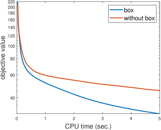
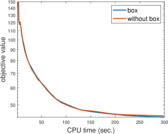
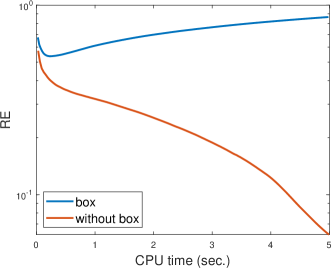
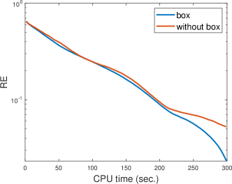
Figure 5: The effects of box constraint on objective values (top) and relative errors (bottom) for MRI (left) and CT (right) reconstruction problems.

In Figure 5, we present algorithmic behaviors of the box constraint for both MRI and CT problems, in which we set jMax to be 5 and 1, respectively (we will discuss the effects of inner iteration number shortly.) In the MRI problem, the box constraint is critical; without it, our algorithm converges to another local minimizer, as RE goes up. With the box constraint, the objective values decrease faster than in the no-box case, and the relative errors drop down monotonically. In the CT case, the influence of box is minor but we can see a faster decay of RE than the no-box case after 200 seconds. In the light of these observations, we only consider the algorithm with a box constraint for the rest of the experiments.

MRI (jMax = 1,3,5,10)	CT (jMax = 1,3,5,10)

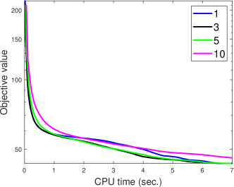
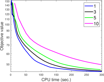
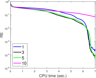
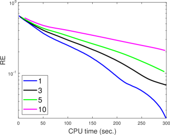
Figure 6: The effects of the maximum number in the inner loops (jMax) on objective values (top) and relative errors (bottom) for MRI (left) and CT (right) reconstruction problems.

We then study the effect of jMax on MRI/CT reconstruction problems in Figure 6. We fix the maximum outer iterations as 300, and examine four possible jMax values: 1, 3, 5 and 10. In the case of MRI, jMax = 10 causes the slowest decay of both objective value and RE. Besides, we observe that only one inner iteration, which is equivalent to our previous approach [18], is not as efficient as more inner iterations to reduce the RE in the MRI problem. The CT results are slightly different, as one inner iteration seems sufficient to yield satisfactory results. The disparate behavior of CT to MRI is probably due to inexact solutions by CG iterations. In other words, more inner iterations do not improve the accuracy. Following Figure 6, we set jMax to be 5 and 1 in MRI and CT, respectively, for the rest of the experiments.

Lastly, we study the sensitivity of the parameters $\lambda,\rho,\beta$ in our proposed algorithm to provide strategies for parameter selection. For simplicity, we set $\gamma=\rho$ as their corresponding auxiliary variables represent $D\mathbf{u}$. In the MRI reconstruction problem, we examine three values of $\lambda\in\{100,1000,10000\}$ and two settings of the number of maximum outer iterations, i.e., kMax $\in\{500,1000\}.$ For each combination of $\lambda$ and kMax, we vary parameters $(\rho,\beta)\in(2^{i},2^{j}),$ for $i,j\in[-4,4],$ and plot the RE in Figure 7. We observe that small values of $\rho$ work well in practice, although we need to assume a sufficiently large value for $\rho$ when proving the convergence results in Theorem 2. Besides, a larger kMax value leads to larger valley regions for the lowest RE, which verifies that only $\rho$ and $\beta$ affect the convergence rate. Figure 7 suggests that our algorithm is generally insensitive to all these parameters $\beta,\rho$ and $\lambda$ as long as $\rho$ is small. Similarly in the CT reconstruction, we set $\lambda\in\{0.005,0.05,0.5\},$ kMax $\in\{100,300\}$, and $(\rho,\beta)\in(2^{i},2^{j}),$ for $i,j\in[-4,4],$ Figure 8 shows that $\rho$ and $\beta$ can be selected in a wide range, especially for large number of outer iterations. But our algorithm is sensitive to $\lambda$ for the CT problem, as $\lambda=0.005$ or $0.5$ yields larger errors than $\lambda=0.05$. In the light of this sensitivity analysis, we can tune parameters by finding the optimal combination among a candidate set for each problem, specifically paying attention to the value of $\lambda$ in the limited-angle CT reconstruction.

$\lambda=100$	$\lambda=1000$	$\lambda=10000$

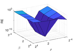
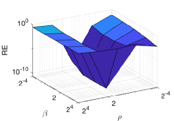
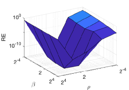
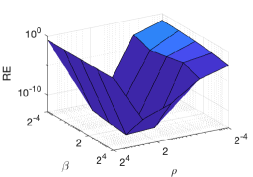
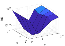
Figure 7: The relative errors with respect to the parameters $\lambda,\rho,\beta$ in Algorithm 1 for MRI reconstruction when kMax is 500 (top) or 1000 (bottom).

$\lambda=0.005$	$\lambda=0.05$	$\lambda=0.5$

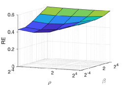
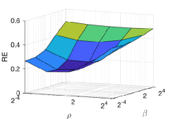
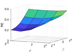
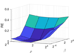
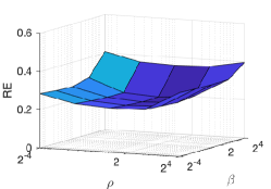
Figure 8: The relative errors with respect to the parameters $\lambda,\rho,\beta$ in Algorithm 1 for CT reconstruction when kMax is 100 (top) or 300 (bottom).

6.2 Super-resolution

We use an original image from [48] of size $688\times 688$ to illustrate the performance of super-resolution. As super-resolution is similar to MRI in the sense of frequency measurements, we set up the maximum iteration number as 5 according to Section 6.1. We restrict the data within a square in the center of the frequency domain (corresponding to low-frequency measurements), and hence varying the sizes of the square leads to different sampling ratios. In addition to regularized methods, we include a direct method of filling in the unknown frequency data by zero, followed by inverse Fourier transform, which is referred to as zero-filling (ZF). The visual results of $1\%$ are presented in Figure 9, showing that both $L_{p}$ and $L_{1}/L_{2}$ are superior over ZF, $L_{1}$, and $L_{1}$-$\alpha L_{2}.$ Specifically, $L_{1}/L_{2}$ can recover these thin rectangular bars, while $L_{1}$ and $L_{1}$-$\alpha L_{2}$ lead to thicker bars with white background, which should be gray. In addition,  $L_{p}$ and $L_{1}/L_{2}$ can recover the most of the letter ‘a’ in the bottom of the image, compared to the other methods, while $L_{1}/L_{2}$ is better than $L_{p}$ with more natural boundaries along the six dots in the middle left of the image. One drawback of $L_{1}/L_{2}$ is that it produces white artifacts near the third square from the left as well as around the letter ‘a’ in the middle. We suspect $L_{1}/L_{2}$ is not very stable, and the box constraint forces the black-and-white regions near edges. We do not present quantitative measures for this example, as four noisy squares on the right of the image lead to meaningless comparison, considering that all the methods return smooth results.

Ground truth	ZF	$L_{1}$
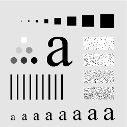
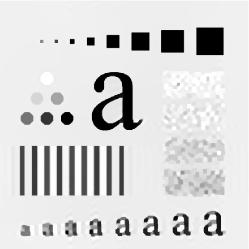
$L_{p}$	$L_{1}$-$\alpha L_{2}$	$L_{1}/L_{2}$

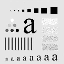
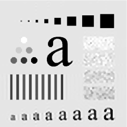
Figure 9: Super-resolution from $1\%$ low frequency data.

6.3 MRI reconstruction

To generate the ground-truth MRI images, we utilize a simulated brain database [49, 50] that has full three-dimensional data volumes obtained by an MRI simulator [51] in different modalities such as T1 and T2 weighted images. As a proof of concept, we extract one slice from the 3D T1 and T2 data as testing images and take frequency data along radial lines. The visual comparisons are presented for 25 radial lines (about 13.74% measurements) in Figure 10. We include the zero-filled method as mentioned in super-resolution, which unfortunately fails to recover the contrast for both T1 and T2. The other regularization methods yield more blurred results than the proposed $L_{1}/L_{2}$ approach. Particularly worth noticing is that our proposed model can effectively separate the gray matter and white matter in the T1 image, as highlighted in the zoom-in regions. Furthermore, we plot the horizontal and vertical profiles in Figure 11, where we can see clearly that the restored profiles via $L_{1}/L_{2}$ are closer to the ground truth than the other approaches, especially near these peaks that can be reached by $L_{p},$ $L_{1}$-$\alpha L_{2},$ and $L_{1}/L_{2}$, but not $L_{1}.$ As a further comparison, we present the MRI reconstruction results under various number of lines (20, 25, and 30) in Table 1, which demonstrates significant improvements of $L_{1}/L_{2}$ over the other models in term of PSNR and RE.

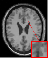
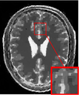
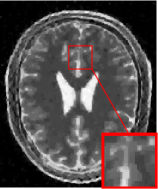
Figure 10: MRI reconstruction from frequency measurements along 25 radial lines of T1 (top row) and T2 (bottom row). From left to right: ground truth, $L_{1}$, $L_{p}$, $L_{1}$-$\alpha L_{2}$, and $L_{1}/L_{2}$.

Figure 11: Horizontal (left) and vertical (right) profiles of MRI reconstruction results from $25$ radial lines for T1 (top) and T2 (bottom).

Table 1: MRI reconstruction from different numbers of radial lines.

Image	Line	ZF		$L_{1}$		$L_{p}$		$L_{1}$-$\alpha L_{2}$		$L_{1}/L_{2}$
		PSNR	RE	PSNR	RE	PSNR	RE	PSNR	RE	PSNR	RE
T1	20	21.26	22.13%	27.20	11.17%	27.24	11.11%	27.41	10.90%	29.94	8.15%
	25	23.42	17.26%	30.32	7.80%	30.06	8.04%	30.34	7.78%	33.21	5.59%
	30	24.07	16.02%	31.92	6.48%	31.63	6.70%	31.70	6.65%	34.84	4.63%
T2	20	17.89	33.91%	21.12	23.37%	21.13	23.34%	21.74	21.75%	23.50	17.76%
	25	18.83	30.44%	22.92	18.99%	23.23	18.33%	23.59	17.58%	25.80	13.63%
	30	19.42	28.43%	24.27	16.26%	24.76	15.36%	25.10	14.78%	27.60	11.09%

6.4 Limited-angle CT reconstruction

Lastly, we examine the limited-angle CT reconstruction problem on two standard phantoms: Shepp-Logan (SL) by Matlab’s built-in command (phantom) and FORBILD (FB) [52]. Notice that the FB phantom has a very low image contrast and we display it with the grayscale window of [1.0, 1.2] in order to reveal its structures; see Figure 12. To synthesize the CT projected data, we discretize both phantoms at a resolution of $256\times 256$. The forward operator $A$ is generated as the discrete Radon transform with a parallel beam geometry sampled at $\theta_{\rm{Max}}/30$ over a range of $\theta_{\rm{Max}}$, resulting in a sub-sampled data of size $362\times 31$. Note that we use the same number of projections when we vary ranges of projection angles. The simulation process is available in the IR and AIR toolbox [53, 54]. Following the discussion in Section 6.1, we set jMax$=1$ for the subproblem. We compare the regularization models with a clinical standard approach, called simultaneous algebraic reconstruction technique (SART) [55].

As the SL phantom has relatively simpler structures than FB, we present an extremely limited angle of only $30^{\circ}$ scanning range in Table 2, which shows that $L_{1}/L_{2}$ achieves significant improvements over SART, $L_{1}$, $L_{p}$, and $L_{1}$-$\alpha L_{2}$ in terms of PSNR and RE. Visually, we present the CT reconstruction results of $45^{\circ}$ projection range for SL (SL-$45^{\circ}$) and $75^{\circ}$ for FB (FB-$75^{\circ}$) in Figure 12. In the first case (SL-$45^{\circ}$), SART fails to recover the ellipse inside of the skull with such a small range of projection angles. All the regularization methods perform much better owing to their sparsity promoting property. However, the $L_{1}$ model is unable to restore the bottom skull and preserve details of some ellipses in the middle. The proposed $L_{1}/L_{2}$ method leads an almost exact recovery with a relative error of $0.64\%$ and visually no difference to the ground truth. In the second case (FB-$75^{\circ}$), we show the reconstructed images with the window of [1.0, 1.2], and observe some fluctuations inside of the skull. $L_{p}$ performs the best, while $L_{1}/L_{2}$ restores the most details of the image among the competing methods. We plot the horizontal and vertical profiles in Figure 13, which illustrates that $L_{1}/L_{2}$ leads to the smallest fluctuations compared to the other methods. We also observe a well-known artifact of the $L_{1}$ method, i.e., loss-of-contrast, as its profile fails to reach the height of jump on the intervals such as $[160,180]$ in the left plot and $[220,230]$ in the right plot of Figure 13, while $L_{1}/L_{2}$ has a good recovery in these regions.

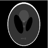
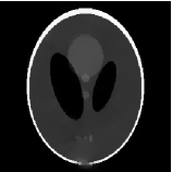
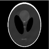
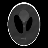
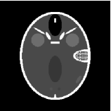
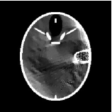
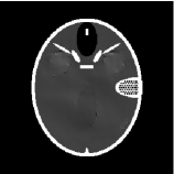
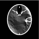
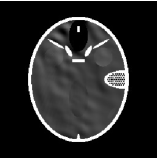
Figure 12: CT reconstruction results of SL-$45^{\circ}$ (top) and FB-$75^{\circ}$ (bottom). From left to right: ground truth, $L_{1}$, $L_{p}$, $L_{1}$-$\alpha L_{2}$, and $L_{1}/L_{2}$. The gray scale window is $[0,1]$ for SL and $[1,1.2]$ for FB.

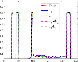
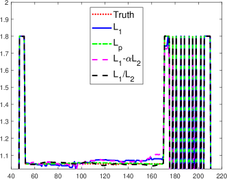
Figure 13: Horizontal and vertical profiles of CT reconstruction results of FB-$75^{\circ}$.

Table 2: CT reconstruction with difference ranges of scanning angles.

phantom	range	SART		$L_{1}$		$L_{p}$		$L_{1}$-$\alpha L_{2}$		$L_{1}/L_{2}$
		PSNR	RE	PSNR	RE	PSNR	RE	PSNR	RE	PSNR	RE
SL	$30^{\circ}$	15.66	66.95%	28.32	15.57%	40.25	3.95%	38.15	5.02%	60.77	0.37%
	$45^{\circ}$	16.08	63.78%	33.33	8.75%	44.06	2.54%	63.34	0.28%	70.42	0.12%
	$60^{\circ}$	16.48	60.92%	43.37	2.75%	46.50	1.92%	80.19	0.04%	73.46	0.09%
FB	$60^{\circ}$	15.61	40.16%	25.43	12.96%	58.01	0.30%	26.24	11.81%	46.97	1.09%
	$75^{\circ}$	16.14	37.79%	28.84	8.76%	59.02	0.27%	29.49	8.13%	49.30	0.83%
	$90^{\circ}$	16.64	35.68%	69.68	0.08%	62.05	0.19%	75.67	0.04%	70.57	0.07%

7 Conclusions and future works

In this paper, we considered the use of $L_{1}/L_{2}$ on the gradient as an objective function to promote sparse gradients for imaging problems. We started from a series of 1D piecewise signal recovery and demonstrated the superiority of the ratio model over $L_{1}$, which is widely known as the total variation. To facilitate the discussion on the empirical evidences, we focused on a constrained model, and proposed a splitting algorithm scheme that has provable convergence for ADMM. We conducted extensive experiments to demonstrate that our approach outperforms the state-of-the-art gradient-based approaches. Motivated by the empirical studies in Section 3, we will devote ourselves to the exact recovery of the TV regularization with respect to the minimum separation of the gradient spikes. We are also interested in extending the analysis to the unconstrained formulation, which is widely applicable in image processing.

References

References

- [1] Rudin L, Osher S, Fatemi E. Nonlinear total variation based noise removal algorithms. Physica D. 1992;60:259–268.
- [2] Bredies K, Kunisch K, Pock T. Total generalized variation. SIAM J Imaging Sci. 2010;3(3):492–526.
- [3] Chen D, Chen YQ, Xue D. Fractional-order total variation image denoising based on proximity algorithm. Appl Math Comput. 2015;257(1):537–545.
- [4] Zhang J, Chen K. A total fractional-Order variation model for image restoration with nonhomogeneous boundary conditions and its numerical solution. SIAM J Imaging Sci. 2015;8(4):2487–2518.
- [5] Osher SJ, Esedoglu S. Decomposition of images by the anisotropic Rudin-Osher-Fatemi model. Comm Pure Appl Math. 2003;57:1609–1626.
- [6] Natarajan BK. Sparse approximate solutions to linear systems. SIAM J Comput. 1995:227–234.
- [7] Candès EJ, Romberg J, Tao T. Stable signal recovery from incomplete and inaccurate measurements. Comm Pure Appl Math. 2006;59:1207–1223.
- [8] Fan J, Li R. Variable selection via nonconcave penalized likelihood and its oracle properties. J Am Stat Assoc. 2001;96(456):1348–1360.
- [9] Zhang C. Nearly unbiased variable selection under minimax concave penalty. Ann Stat. 2010:894–942.
- [10] Zhang T. Multi-stage convex relaxation for learning with sparse regularization. In: Adv. Neural. Inf. Process. Syst.; 2009. p. 1929–1936.
- [11] Shen X, Pan W, Zhu Y. Likelihood-based selection and sharp parameter estimation. J Am Stat Assoc. 2012;107(497):223–232.
- [12] Lou Y, Yin P, Xin J. Point source super-resolution via non-convex based methods. J Sci Comput. 2016;68:1082–1100.
- [13] Lv J, Fan Y. A unified approach to model selection and sparse recovery using regularized least squares. Ann Appl Stat. 2009:3498–3528.
- [14] Zhang S, Xin J. Minimization of transformed penalty: closed form representation and iterative yhresholding algorithms. Comm Math Sci. 2017;15:511–537.
- [15] Zhang S, Xin J. Minimization of transformed penalty: theory, difference of convex function algorithm, and robust application in compressed sensing. Math Program. 2018;169:307–336.
- [16] Chartrand R. Exact reconstruction of sparse signals via nonconvex minimization. IEEE Signal Process Lett. 2007;10(14):707–710.
- [17] You J, Jiao Y, Lu X, Zeng T. A nonconvex model with minimax concave penalty for image restoration. J Sci Comput. 2019;78(2):1063–1086.
- [18] Rahimi Y, Wang C, Dong H, Lou Y. A scale invariant approach for sparse signal recovery. SIAM J Sci Comput. 2019;41(6):A3649–A3672.
- [19] Wang C, Yan M, Rahimi Y, Lou Y. Accelerated schemes for the minimization. IEEE Trans Signal Process. 2020;68:2660–2669.
- [20] Tao M. Minimization of L1 over L2 for sparse signal recovery with convergence guarantee; 2020. http://www.optimization-online.org/DB_HTML/2020/10/8064.html.
- [21] Wang C, Tao M, Nagy J, Lou Y. Limited-angle CT reconstruction via the minimization. SIAM J Imaging Sci. 2021;14(2):749–777.
- [22] Candès EJ, Fernandez-Granda C. Super-resolution from noisy data. J Fourier Anal Appl. 2013;19(6):1229–1254.
- [23] Boyd S, Parikh N, Chu E, Peleato B, Eckstein J. Distributed optimization and statistical learning via the alternating direction method of multipliers. Found Trends Mach Learn. 2011 Jan;3(1):1–122.
- [24] Lou Y, Zeng T, Osher S, Xin J. A weighted difference of anisotropic and isotropic total variation model for image processing. SIAM J Imaging Sci. 2015;8(3):1798–1823.
- [25] Yin P, Esser E, Xin J. Ratio and Difference of and Norms and Sparse Representation with Coherent Dictionaries. Comm Info Systems. 2014;14:87–109.
- [26] Lou Y, Yin P, He Q, Xin J. Computing sparse representation in a highly coherent dictionary based on difference of and . J Sci Comput. 2015;64(1):178–196.
- [27] Ma T, Lou Y, Huang T. Truncated - models for sparse recovery and rank minimization. SIAM J Imaging Sci. 2017;10(3):1346–1380.
- [28] Lou Y, Yan M. Fast - minimization via a proximal operator. J Sci Comput. 2018;74(2):767–785.
- [29] Guo K, Han D, Wu T. Convergence of alternating direction method for minimizing sum of two nonconvex functions with linear constraints. Int J of Comput Math. 2017;94(8):1653–1669.
- [30] Pang JS, Tao M. Decomposition methods for computing directional stationary solutions of a class of nonsmooth nonconvex optimization problems. SIAM J Optim. 2018;28(2):1640–1669.
- [31] Wang Y, Yin W, Zeng J. Global convergence of ADMM in nonconvex nonsmooth optimization. J Sci Comput. 2019;78(1):29–63.
- [32] Candès EJ, Fernandez-Granda C. Towards a mathematical theory of super-resolution. Comm Pure Appl Math. 2014;67(6):906–956.
- [33] Grant M, Boyd S. CVX: Matlab Software for Disciplined Convex Programming, version 2.1; 2014. http://cvxr.com/cvx.
- [34] Donoho DL. Superresolution via sparsity constraints. SIAM J Math Anal. 1992;23(5):1309–1331.
- [35] Morgenshtern VI, Candes EJ. Super-resolution of positive sources: The discrete setup. SIAM Journal on Imaging Sciences. 2016;9(1):412–444.
- [36] Chan RH, Ma J. A multiplicative iterative algorithm for box-constrained penalized likelihood image restoration. IEEE Trans Image Process. 2012;21(7):3168–3181.
- [37] Kan K, Fung SW, Ruthotto L. PNKH-B: A Projected Newton-Krylov Method for Large-Scale Bound-Constrained Optimization. arXiv preprint arXiv:200513639. 2020.
- [38] Nocedal J, Wright SJ. Numerical Optimization. Springer; 2006.
- [39] Bolte J, Daniilidis A, Lewis A. The Łojasiewicz inequality for nonsmooth subanalytic functions with applications to subgradient dynamical systems. SIAM J Optim. 2007;17(4):1205–1223.
- [40] Li G, Pong TK. Global convergence of splitting methods for nonconvex composite optimization. SIAM J Optim. 2015;25(4):2434–2460.
- [41] Attouch H, Bolte J, Redont P, Soubeyran A. Proximal alternating minimization and projection methods for nonconvex problems: An approach based on the Kurdyka-Łojasiewicz inequality. Mathematics of operations research. 2010;35(2):438–457.
- [42] Candès EJ, Romberg J, Tao T. Robust uncertainty principles: Exact signal reconstruction from highly incomplete frequency information. IEEE Trans Inf Theory. 2006;52(2):489–509.
- [43] Avinash C, Malcolm S. Principles of computerized tomographic imaging. Philadelphia, PA, USA: Society for Industrial and Applied Mathematics; 2001.
- [44] Chen Z, Jin X, Li L, Wang G. A limited-angle CT reconstruction method based on anisotropic TV minimization. Phys Med Biol. 2013;58(7):2119.
- [45] Zhang Y, Chan HP, Sahiner B, Wei J, Goodsitt MM, Hadjiiski LM, et al. A comparative study of limited-angle cone-beam reconstruction methods for breast tomosynthesis. Med Phys. 2006;33(10):3781–3795.
- [46] Wang Z, Huang Z, Chen Z, Zhang L, Jiang X, Kang K, et al. Low-dose multiple-information retrieval algorithm for X-ray grating-based imaging. Nucl Instrum Methods Phys. 2011;635(1):103–107.
- [47] Xu Z, Chang X, Xu F, Zhang H. Regularization: A Thresholding Representation Theory and a Fast Solver. IEEE Trans Neural Netw Learn Syst. 2012;23:1013–1027.
- [48] Gonzalez RC, Woods RE, Eddins SL. Digital image processing using MATLAB. Pearson Education India; 2004.
- [49] Cocosco CA, Kollokian V, Kwan RKS, Pike GB, Evans AC. BrainWeb: Online Interface to a 3D MRI Simulated Brain Database. NeuroImage. 1997;5:425.
- [50] Kwan RS, Evans AC, Pike GB. MRI simulation-based evaluation of image-processing and classification methods. IEEE Trans Med Imaging. 1999;18(11):1085–1097.
- [51] Kwan RKS, Evans AC, Pike GB. An extensible MRI simulator for post-processing evaluation. In: International Conference on Visualization in Biomedical Computing. Springer; 1996. p. 135–140.
- [52] Yu Z, Noo F, Dennerlein F, Wunderlich A, Lauritsch G, Hornegger J. Simulation tools for two-dimensional experiments in x-ray computed tomography using the FORBILD head phantom. Phys Med Biol. 2012;57(13):N237.
- [53] Gazzola S, Hansen PC, Nagy JG. IR Tools: a MATLAB package of iterative regularization methods and large-scale test problems. Numer Algorithms. 2019;81(3):773–811.
- [54] Hansen PC, Saxild-Hansen M. AIR tools — MATLAB package of algebraic iterative reconstruction methods. J Comput Appl Math. 2012;236(8):2167–2178.
- [55] Andersen AH, Kak AC. Simultaneous algebraic reconstruction technique (SART): a superior implementation of the ART algorithm. Ultrason Imaging. 1984;6(1):81–94.